Neural Models for Sequence Chunking

Abstract

Many natural language understanding (NLU) tasks, such as shallow parsing (i.e., text chunking) and semantic slot filling, require the assignment of representative labels to the meaningful chunks in a sentence. Most of the current deep neural network (DNN) based methods consider these tasks as a sequence labeling problem, in which a word, rather than a chunk, is treated as the basic unit for labeling. These chunks are then inferred by the standard IOB (Inside-Outside-Beginning) labels. In this paper, we propose an alternative approach by investigating the use of DNN for sequence chunking, and propose three neural models so that each chunk can be treated as a complete unit for labeling. Experimental results show that the proposed neural sequence chunking models can achieve start-of-the-art performance on both the text chunking and slot filling tasks.

Introduction

Semantic slot filling and shallow parsing which are standard NLU tasks fall under the umbrella of natural language understanding (NLU), which are usually solved by labeling meaningful chunks in a sentence. This kind of task is usually treated as a sequence labeling problem, where every word in a sentence is assigned an IOB-based (Inside-Outside-Beginning) label. For example, in Figure  1, in the sentence “But it could be much worse” we label “could” as B-VP, “be” as I-VP, and “it” as B-NP, while “But” belongs to an artificial class O. This labeling indicates that a chunk “could be” is a verb phrase (VP) where the label prefix B means the beginning word of the chunk, while I refers to the other words within the same semantic chunk; and “it” is a single-word chunk with NP label.

Such sequence labeling forms the basis for many recent deep network based approaches, e.g., convolutional neural networks (CNN), recurrent neural networks (RNN) or its variation, long short-term memory networks (LSTM). RNN and LSTM are good at capturing sequential information (?; ?; ?; ?; ?; ?; ?), whereas CNN can extract effective features for classification (?; ?).

Most of the current DNN based approaches use the IOB scheme to label chunks. However, this approach of these labels has a few drawbacks. First, we don’t have an explicit model to learn and identify the scope of chunks in a sentence, instead we infer them implicitly (by IOB labels). Hence the learned model might not be able to fully utilize the training data which could result in poor performance. Second, some neural networks like RNN or LSTM have the ability to encode context information but don’t treat each chunk as a complete unit. If we can eliminate this drawback, it could result in more accurate labeling, especially for multi-word chunks.

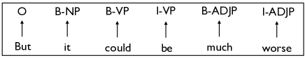
Figure 1: An example of text chunking where each word is labeled using the IOB scheme. The chunk “could be” is a verb phrase (VP) and “it” is a single-word chunk with NP label.

Sequence chunking is a natural solution to overcome the two drawbacks mentioned before. In sequence chunking, the original sequence labeling task is divided into two sub-tasks: (1) Segmentation, to identify scope of the chunks explicitly; (2) Labeling, to label each chunk as a single unit based on the segmentation results.

? (2016) used a stack-LSTM (?) and a transition-based algorithm for sequence chunking. In their paper, the segmentation step is based on shift-reduce parser based actions. In this paper, we propose an alternative approach by relying only on the neural architectures for NLU. We investigate two different ways for segmentation: (1) using IOB labels; and (2) using pointer networks (?) and propose three neural sequence chunking models. Pointer network performs better than the model using IOB. In addition, it also achieves state-of-the-art performance on both text chunking and slot filling tasks.

Basic Neural Networks

Recurrent Neural Network

Recurrent neural network (RNN) is a neural network that is suitable for modeling sequential information. Although theoretically it is able to capture long-distance dependencies, in practice it suffers from the gradient vanishing/exploding problems (?). Long short-term memory networks (LSTM) were introduced to cope with these gradient problems and model long-range dependencies (?) by using a memory cell. Given an input sentence $x=(x_{1},x_{2},...,x_{T})$ where $T$ is the sentence length, LSTM hidden state at timestep $t$ is computed by:

$$\begin{split}i_{t}&=\sigma(W^{i}x_{t}+U^{i}h_{t-1}+b^{i})\\ f_{t}&=\sigma(W^{f}x_{t}+U^{f}h_{t-1}+b^{f})\\ o_{t}&=\sigma(W^{o}x_{t}+U^{o}h_{t-1}+b^{o})\\ g_{t}&=tanh(W^{g}x_{t}+U^{g}h_{t-1}+b^{g})\\ c_{t}&=f_{t}\odot c_{t-1}+i_{t}\odot g_{t}\\ h_{t}&=o_{t}\odot tanh(c_{t})\end{split}$$ (1)

where $\sigma(\cdot)$ and tanh$(\cdot)$ are the element-wise sigmoid and hyperbolic tangent functions, $\odot$ is the element-wise multiplication operator, and $i_{t}$,$f_{t}$,$o_{t}$ are the input, forget and output gates. $h_{t-1}$ and $c_{t-1}$ are the hidden state and memory cell of previous timestep respectively. To simplify the notation, we use $x_{t}$ to denote both the word and its embedding.

The bi-directional LSTM (Bi-LSTM), a modification of the LSTM, consists of a forward and a backward LSTM. The forward LSTM reads the input sentence as it is (from $x_{1}$ to $x_{T}$) and computes the forward hidden states ($\overrightarrow{h_{1}},\overrightarrow{h_{2}},...,\overrightarrow{h_{T}}$), while the backward LSTM reads the sentence in the reverse order (from $x_{T}$ to $x_{1}$), and creates backward hidden states ($\overleftarrow{h_{1}},\overleftarrow{h_{1}},...,\overleftarrow{h_{T}}$). Then for each timestep $t$, the hidden state of the Bi-LSTM is generated by concatenating $\overrightarrow{h_{t}}$ and $\overleftarrow{h_{t}}$,

$$\overleftrightarrow{h_{t}}=[\overrightarrow{h_{t}};\overleftarrow{h_{t}}]$$ (2)

Convolutional Neural Network

Convolutional Neural Networks (CNN) have been used to extract features for sentence classification (?; ?; ?). Given a sentence, a CNN with m filters and a filter size of n extracts a m-dimension feature vector from every n-gram phrase of the sentence. A max-over-time pooling (max-pooling) layer is applied over all extracted feature vectors to create the final indicative feature vector (m-dimension) for the sentence.

Following this approach, we use CNN and max-pooling layer to extract features from chunks. For each identified chunk, we first apply CNN to the embedding of its words (irrespective of it being a single-word chunk or chunk), and then use the max-pooling layer on top to get the chunk feature vector for labeling. We use CNNMax to denote the two layers hereafter.

Proposed Models

In this section, we introduce the different neural models for sequence chunking and discuss the final learning objective.

Model I

For segmentation, the most straightforward and intuitive way is to transform it into a sequence labeling problem with 3 classes : I - inside, O - outside, B - beginning; and then understand the scope of the chunks from these labels. Building on this, we propose Model I, which is a Bi-LSTM as shown in Figure 2. In the model, we take the bi-LSTM hidden states generated by Formula (2) as features for both segmentation and labeling.

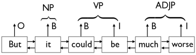
Figure 2: Model I: Single Bi-LSTM model for both segmentation and labeling subtasks.

For example, we first classify each word into an IOB label as shown in (Figure 2). Suppose a chunk begins at word $i$ with length $l$ (with one B label and followed by $(l-1)$ I labels), then we can compute a feature vector for a chunk as follows:

$$Ch_{j}=Average(\overleftrightarrow{h_{i}},\overleftrightarrow{h_{i+1}},...,\overleftrightarrow{h_{i+l-1}})$$ (3)

where $j$ is the chunk index of the sentence, and $Average(\cdot)$ computes the average of the input vectors. With $Ch_{j}$, we apply a softmax layer over all chunk labels for labeling. For example in Figure 2, “much worse” is identified as a chunk with length 2; and we apply Formula (3) on its hidden states, to finally get the “ADJP” label.

Model II

A drawback of Model I is that a single Bi-LSTM may not perform well on both segmentation and labeling subtasks. To overcome this we propose Model II, which follows the encoder-decoder framework ( Figure  3) (?; ?). Similar to Model I, we employ a Bi-LSTM for segmentation with IOB labels. This Bi-LSTM will also serve as an encoder and create a sentence representation $[\overrightarrow{h_{T}};\overleftarrow{h_{1}}]$ (by concatenating the final hidden state of the forward and backward LSTM) which is used to initialize the decoder LSTM.

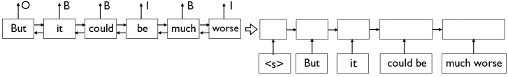
Figure 3: Model II: Encoder-decoder framework. The encoder Bi-LSTM is used for segmentation and the decoder LSTM is used for labeling.

We modify the general encoder-decoder framework and use chunks as the inputs instead of words. For example, much worse is a chunk in Figure 3, and we take it as a single input to the decoder. The input chunk representation $C_{j}$ consists of several parts. We first use the CNNMax layer to extract important information from words inside the chunk:

$$Cx_{j}=g(x_{i},x_{i+1},...,x_{i+l-1})$$ (4)

where $g(\cdot)$ is the CNNMax layer. Then we use the context word embeddings of the chunk to capture context information (?; ?; ?). The context window size is a hyperparameter to tune. Finally, we average the hidden states from the encoder Bi-LSTM by Formula (3). By using these three parts, we extract different useful information for labeling, and import them all into the decoder LSTM. Thus, the decoder LSTM hidden state is updated by:

$$h_{j}=\textit{LSTM}(Cx_{j},Ch_{j},Cw_{j},h_{j-1},c_{j-1})$$ (5)

here $Cw_{j}$ is the concatenation of context word embeddings. Note that the computation of hidden states here is similar to Formula (1), the only difference is that here we have three inputs $\{Cx_{j},Ch_{j},Cw_{j}\}$. The generated hidden states are finally used for labeling by a softmax layer.

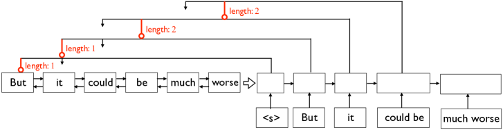
Figure 4: Model III: Encoder-decoder-pointer framework : Segmentation is done by a pointer network and a decoder LSTM is used for labeling.

Model III

There are two drawbacks of using IOB labels for segmentation. First, it is hard to use chunk-level features for segmentation, like the length of chunks. Also, using IOB labels cannot compare different chunks directly. The shift-reduce algorithm used in (?) has the same issue. They both transform a multi-class classification problem (we could have a lot of chunk candidates) into a 3-class classification problem, in which the chunks are inferred implicitly.

To resolve this problem, we further propose Model III, which is an encoder-decoder-pointer framework (Figure 4) (?). Model III is similar to Model II, the only difference being the method of identifying chunks.

Model III is a greedy process of segmentation and labeling, where we first identify one chunk, and then label it. This process is repeated until all the words are processed. As all chunks are adjacent to each other , after one chunk is identified, the beginning point of the next one is also known, and only its ending point is to be determined. We adopt pointer network (?) to do this. For a possible chunk beginning at timestep $b$, we first generate a feature vector for each possible ending point candidate $i$:

$$\begin{split}u^{i}_{j}=&\ v_{1}^{T}tanh(W_{1}\overleftrightarrow{h_{i}}+W_{2}x_{i}+W_{3}x_{b}+W_{4}d_{j})\\ &+\ v_{2}^{T}LE(i-b+1)\ \ \ \ \ \ \ \ \ \ \ \ \ \ \ i\in[b,b+l_{m})\end{split}$$ (6)

where $j$ is the decoder timestep (i.e., chunk index), $l_{m}$ is the maximum chunk length. We use the encoder hidden state $\overleftrightarrow{h_{i}}$, the ending point candidate word embedding $x_{i}$, together with current beginning word embedding $x_{b}$ and decoder hidden state $d_{j}$ as features. We also use the chunk length embedding, $LE(i-b+1)$, as the chunk level feature. $W_{1}$,$W_{2}$,$W_{3}$,$W_{4}$,$v_{1}$,$v_{2}$ and $LE$ are all learnable parameters. Then the probability of choosing ending point candidate $i$ is:

$$p(i)=\frac{exp(u^{i}_{j})}{\sum_{k=b}^{b+l_{m}-1}exp(u^{k}_{j})}$$ (7)

We use this probability to identify the scope of chunks. For example, suppose we just identified word it as a one word chunk with label NP in Figure 4. Following the line emitted from it, we will need to decide the ending point of the next chunk (the beginning point is obviously the word could after it). With the maximum chunk length 2, we have two choices, one is to stop at word could and gets a one word chunk could, and the other is to stop at word be and generates a two word chunk could be. From the figure, we can see that the model selects the second case (red circle part), and creates a two word chunk. This chunk will serve as the input of the next decoder timestep. The decoder hidden states are updated similar to Model II (Equation 5).

Learning Objective

As we described above, all the aforementioned models solve two subtasks - segmentation and labeling. We use the cross-entropy loss function for both the two subtasks, and sum the two losses to form the the learning objective:

$$L(\theta)=L_{segmentation}(\theta)+L_{labeling}(\theta)$$ (8)

where $\theta$ denotes the learnable parameters. Alternatively, we could also use weighted sum, or do multi-task learning by considering segmentation and labeling as the two tasks. We leave these extensions as future work.

Experiments

Experimental Setup

We conduct experiments on text chunking and semantic slot filling respectively to test the performance of the neural sequence chunking models we propose in this paper. Both these tasks identify the meaningful chunks in the sentence, such as the noun phrase (NP), or the verb phrase (VP) for text chunking in Figure 1, and the “depart_city” for slot filling task in Figure 5.

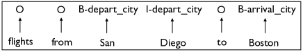
Figure 5: An example of semantic slot filling using the IOB scheme. “San Deigo” is a multi-word chunk with label “depart_city”.

We use the CoNLL 2000 shared task (?) dataset for text chunking. It contains 8,936 training and 893 test sentences. There are 12 different labels (22 with IOB prefix included). Since it doesn’t have a validation set, we hold out 10% of the training data (selected at random) as the validation set.

To evaluate the effectiveness of our method on the semantic slot filling task, we use two different datasets. The first one is the ATIS dataset, which consists of reservation requests from the air travel domain. It contains 4,978 training and 893 testing sentences in total, with a vocabulary size of 572. There are 84 different slot labels (127 if with IOB prefix). We randomly selected 80% of the training data for model training and the rest 20% as the validation set (?). Following the work of (?), we also use a larger dataset by combining the ATIS corpus with the MIT Restaurant Corpus and MIT Movie Corpus (?; ?). This dataset has 30,229 training and 6,810 testing instances. Similar to the previous dataset, we use 80% of the training instances for training the model, and treat the rest 20% as a validation set. This dataset has a vocabulary size of 16,049 and the number of slot labels is 116 (191 with IOB prefix included). Since this dataset is considerably larger and includes 3 different domains, we use “LARGE” to denote it hereafter.

The final performance is measured in terms of F1-score, computed by the public available script conlleval.pl . We report the F1-score on the test set with parameters that achieves the best F1-score on the validation set. Towards the neural sequence chunking models, after we get the label for each chunk, we will assign each of its word an IOB-based label accordingly so that the script can do evaluation. We also report the segmentation F1-score to assess the segmentation performance of different models. This is also computed by the conlleval.pl script, but only considers three labels, i.e. {I,O,B}. To compute the segmetnation F1-score, we delete the content label for each word, for example, if a word has a label “B-VP”, we will delete “VP” and the left “B” is used for segmentation F1-score.

For the two tasks, we use hidden state size as 100 for the forward and backward LSTM respectively in Bi-LSTM, and size 200 for the LSTM decoder. We use dropout with rate 0.5 on both the input and output of all LSTMs. The mini-batch size is set to 1. The number of training epochs are limited to 200 for text chunking, and 100 for slot filling. For the CNN used in Model II and III on extracting chunk features, the filter size is the same as word embedding dimension, and the filter window size as 2. We adopt SGD to train the model, and by grid search, we tune the initial learning rate in [0.01, 0.1], learning rate decay in [1e-6, 1e-4], and context window size {1,3,5}.

For the word embedding, following (?), we don’t use pre-trained embedding for the slot filling task, but use a randomly initialized embedding and tune the dimension in $\{30,50,75\}$ by grid search. For text chunking, we concatenate two different embeddings. The first is SENNA embedding (?) with dimension 50. The other is a word representation generated based on its composed characters. we adopt a CNN onto the randomly initialized character embeddings, with 30 filters and filter window size 3.

Text Chunking Results

Results on the text chunking task are shown in Table 1. In this, the “baseline (Bi-LSTM)” refers to a Bi-LSTM model for sequence labeling (use IOB-based labels on words as in Figure 1). “F1” is the final evaluation metric, and “segment-F1” refers to the segmentation F1-score. From the table, we can see that Model I and Model II only have comparable results with the baseline on both evaluation metrics - segment-F1 and final F1 score. Hence, we infer that using IOB labels to do segmentation independently might not be a good choice. However, Model III outperforms the baseline on both segmentation and labeling.

	F1	Segment-F1
baseline (Bi-LSTM)	94.13	95.28
Model I	94.01	95.09
Model II	94.13	95.22
Model III	94.72	95.75

Table 1: Text chunking results of our neural sequence chunking models.

We further compare our best result with the current published results in Table 2. In the table, (?) is the first work of using neural networks for text chunking. ? used a BiLSTM-CRF framework together with a lot of handcraft features. ? extend this framework and employ a GRU to incorporate the character information of words, rather than using handcrafted features. To our best knowledge, they got the current best results 94.66 on the text chunking task. Different from previous work, we model the segmentation part explicitly in our neural models, and without using CRF, we get a state-of-the-art performance of 94.72.

Methods	F1-score
SVM Classifier (?)	93.48
SVM Classifier (?)	93.91
Second order CRF (?)	94.30
HMM + voting scheme (?)	94.01
Conv network tagger (senna) (?)	94.32
BiLSTM-CRF (?)	94.46
BiGRU-CRF (?)	94.66
Model III (Ours)	94.72

Table 2: Comparison with published results on the CoNLL chunking dataset.

Slot Filling Results

Segmentation Results

	ATIS		LARGE
	F1	Segment-F1	F1	Segment-F1
baseline (Bi-LSTM)	95.23	98.85	75.73	80.79
Model I	95.25	98.92	76.68	79.93
Model II	95.71	98.82	77.26	79.99
Model III	95.86	99.01	78.49	82.44

Table 3: Main results of our neural sequence chunking models on slot filling task.

From the Table 3, we can see that the segment-F1 score on ATIS data is much better than the one on LARGE data ($\sim$99% vs. $\sim$80%). This is because the ATIS data is much easier for segmentation than LARGE data. As shown in Table 4, more than 97% of the chunks in ATIS data have only one or two words, while the LARGE data has much longer chunks. Also, compared to the small ATIS vocabulary (572 words), it is harder to learn a good segmentation model with a more complicated vocabulary (about 16k words) in LARGE data.

	ATIS		LARGE
	Train	Test	Train	Test
1	10275 (77.7%)	2096 (73.9%)	28511 (46.8%)	7283 (42.8%)
2	2726 (20.6%)	659 (23.2%)	20679 (34.0%)	6214 (36.5%)
$>=$3	224 (1.7%)	82 (2.9%)	11694 (19.2%)	3516 (20.7%)

Table 4: Statistics on the length of chunks: The first column denotes chunk-lengths. For example, first cell indicates that there are 10275 chunks of length 1, and accounts for 77.7% of all ATIS chunks.

Moreover, Model III gets the best segmentation performance over all the models (99.01% and 82.44%), confirming that our pointer network in model III is good at this task. However, Model I and II are comparable to baseline on the easy ATIS data, and are about 1% worse on LARGE data. This further confirms our analysis on text chunking experiments that using IOB labels alone for segmentation, (like in Model I and II) cannot give us a good result.

	ATIS			LARGE
	1	2	$>=$3	1	2	$>=$3
Baseline(Bi-LSTM)	98.90	98.70	98.78	86.25	88.48	54.88
Model I	98.95	98.78	99.39	85.91	87.27	53.30
Model II	98.83	98.78	98.78	86.42	87.29	52.98
Model III	99.00	98.93	100.0	89.01	88.69	56.59

Table 5: Segment-F1 on different chunk-lengths.

We further investigate the segmentation process and show the segmentation F1-score on different chunk lengths in Table 5. The results demonstrate that the poor performance on LARGE data is mainly due to the bad performance on identifying long chunks (around 55%). Our Model III improves this score by  2% over baseline (54.88% vs. 56.59%). As the absolute performance on this subset is still low, future research efforts should focus on improving this performance. In addition, Model I and II get comparable segmentation results with the baseline model on one-words chunks, while being worse on longer chunks, further supporting this analysis.

Labeling Results

From Table 3, we observe that Model III has the best F1 score as compared to the baseline and other neural chunking models. Another observation is that Model I and II get better improvements over baseline even though they are poor at segmentation in slot filling task.

	ATIS			LARGE
	1	2	$>=$3	1	2	$>=$3
baseline(Bi-LSTM)	95.37	96.03	85.19	79.21	83.56	53.36
Model I	95.23	96.18	88.48	83.10	82.35	51.76
Model II	95.87	96.18	87.80	85.01	82.82	51.15
Model III	95.89	96.19	92.68	84.97	83.89	54.38

Table 6: F1-scores for different chunk-lengths

Table 6 gives some insights on this by showing the F1-score on different chunk-lengths. Comparing Table 5 and 6, we can see when Model I and II achieve comparable segment-F1 with baseline, and the F-1 scores are higher. For slot filling task, the joint learning framework (Formula (8)) helps labeling while harms segmentation on model I and II. Moreover, the usage of encoder in Model II could also help labeling in this task (?). Finally, our Model III could achieve better F1 score on all chunk lengths.

Comparison with Published Results

We compare the ATIS results of our best model (Model III) with current published results in Table 7. As shown in the table, many researchers have done a lot of work which uses deep neural networks for slot filling. Recent work shows the ranking loss is helpful (?), and adding encoder improves the score to 95.66%. The best published result in the table is from (?), which is 95.79%. Compared with previous results, our Model III gets the state-of-the-art performance 95.86%.

Methods	F1-score
RNN (?)	94.11
CNN-CRF (?)	94.35
Bi-RNN (?)	94.73
LSTM (?)	94.85
RNN-SOP (?)	94.89
Deep LSTM (?)	95.08
RNN-EM (?)	95.25
Bi-RNN with ranking loss (?)	95.56
Sequential CNN (?)	95.61
Encoder-labeler Deep LSTM (?)	95.66
BiLSTM-LSTM (focus) (?)	95.79
Model III (Ours)	95.86

Table 7: Comparison with published results on the ATIS data

We compare our approach against the only set of published results on the LARGE data from (?), against which we compare our approach. The reported F1 score on this dataset by their encoder-decoder model is 74.41, and our best model achieves a score of 78.49 which is significantly higher.

Related Work

In recent years, many deep learning approaches have been explored for resolving the sequence labeling tasks. (?) proposed an effective window-based approach, in which they used a feed-forward neural network to classify each word and conditional random fields (CRF) to capture the sequential information. CNNs are also widely used for extracting effective classification features (?; ?).

RNNs are a straightforward and better suited choice for these tasks as they model sequential information. (?) presented a BiLSTM-CRF model, and achieved state-of-the-art performance on several tasks, like named entity recognition and text chunking with the help of handcrafted features. (?) used a BiLSTM for labeling and a CNN to capture character-level information, like (?) and additionally used handcrafted features to gain good performance. Many works have then been investigated to combine the advantages of the above two works and achieved state-of-the-art performance without handcrafted features. These works usually use a BiLSTM or BiGRU as the major labeling architecture, and a LSTM or GRU or CNN to capture the character-level information, and finally a CRF layer to model the label dependency (?; ?; ?).

In addition, many similar works have also been explored for slot filling, like RNN (?; ?), LSTM (?; ?), adding external memory (?), adding encoder (?), using ranking loss (?), adding attention (?) and so on.

In the other direction, people also developed neural networks to help traditional sequence processing methods, like CRF parsing (?) and weighted finite-state transducer (?).

Conclusion

In this paper, we presented three different models for sequence chunking. Our experiments show that the segmentation results of Model I and Model II are comparable to baseline on text chunking data and ATIS data, and worse than the baseline on LARGE data, while Model III gains higher segment-F1 score than baseline, demonstrating that the use of IOB labels is not suitable for building segmentation models independently. Moreover, Model I and II do not give consistent improvements on the final F1 score - the segmentation step improves labeling on slot filling, but not on the text chunking task. Finally, Model III consistently performs better than baseline and gets state-of-the-art performance on the two tasks. We also gain insights about the datasets we use by comparing the segment-F1 scores and F1 scores of model III. For the text chunking data (95.75 vs. 94.72) and LARGE data (82.44 vs. 78.49), the scores are close to each other, indicating that segmentation is a major challenge in these two datasets compared to labeling. But for ATIS data (99.01 vs. 95.86), the segmentation score is almost 100 percent, so labeling seems like the main challenge in this dataset. We hope this insight encourages more research efforts on the similar tasks. Finally, the proposed neural sequence chunking models achieves state-of-the-art performance on both text chunking and slot filling.

References

- [Bahdanau, Cho, and Bengio 2014] Bahdanau, D.; Cho, K.; and Bengio, Y. 2014. Neural machine translation by jointly learning to align and translate. arXiv preprint arXiv:1409.0473.
- [Bengio, Simard, and Frasconi 1994] Bengio, Y.; Simard, P.; and Frasconi, P. 1994. Learning long-term dependencies with gradient descent is difficult. IEEE transactions on neural networks 5(2):157–166.
- [Chiu and Nichols 2015] Chiu, J. P., and Nichols, E. 2015. Named entity recognition with bidirectional lstm-cnns. arXiv preprint arXiv:1511.08308.
- [Collobert et al. 2011] Collobert, R.; Weston, J.; Bottou, L.; Karlen, M.; Kavukcuoglu, K.; and Kuksa, P. 2011. Natural language processing (almost) from scratch. Journal of Machine Learning Research 12(Aug):2493–2537.
- [dos Santos and Gatti 2014] dos Santos, C. N., and Gatti, M. 2014. Deep convolutional neural networks for sentiment analysis of short texts. In COLING, 69–78.
- [dos Santos, Xiang, and Zhou 2015] dos Santos, C.; Xiang, B.; and Zhou, B. 2015. Classifying relations by ranking with convolutional neural networks. In ACL, 626–634. Beijing, China: Association for Computational Linguistics.
- [Durrett and Klein 2015] Durrett, G., and Klein, D. 2015. Neural crf parsing. In Proceedings of ACL 2015, 302–312.
- [Dyer et al. 2015] Dyer, C.; Ballesteros, M.; Ling, W.; Matthews, A.; and Smith, N. A. 2015. Transition-based dependency parsing with stack long short-term memory. In Proceedings of ACL 2015, 334–343.
- [Hochreiter and Schmidhuber 1997] Hochreiter, S., and Schmidhuber, J. 1997. Long short-term memory. Neural computation 9(8):1735–1780.
- [Huang, Xu, and Yu 2015] Huang, Z.; Xu, W.; and Yu, K. 2015. Bidirectional lstm-crf models for sequence tagging. arXiv preprint arXiv:1508.01991.
- [Jaech, Heck, and Ostendorf 2016] Jaech, A.; Heck, L.; and Ostendorf, M. 2016. Domain adaptation of recurrent neural networks for natural language understanding. arXiv preprint arXiv:1604.00117.
- [Kim 2014] Kim, Y. 2014. Convolutional neural networks for sentence classification. arXiv preprint arXiv:1408.5882.
- [Kudo and Matsumoto 2001] Kudo, T., and Matsumoto, Y. 2001. Chunking with support vector machines. In Proceedings of NAACL 2001, 1–8. Association for Computational Linguistics.
- [Kudoh and Matsumoto 2000] Kudoh, T., and Matsumoto, Y. 2000. Use of support vector learning for chunk identification. In Proceedings of the 2nd Workshop on Learning Language in Logic and the 4th Conference on Computational Natural Language Learning - Volume 7, ConLL ’00, 142–144.
- [Kurata et al. 2016] Kurata, G.; Xiang, B.; Zhou, B.; and Yu, M. 2016. Leveraging sentence-level information with encoder lstm for semantic slot filling. arXiv preprint arXiv:1601.01530.
- [Lample et al. 2016] Lample, G.; Ballesteros, M.; Kawakami, K.; Subramanian, S.; and Dyer, C. 2016. Neural architectures for named entity recognition. In In proceedings of NAACL 2016.
- [Liu and Lane 2015] Liu, B., and Lane, I. 2015. Recurrent neural network structured output prediction for spoken language understanding. In Proc. NIPS Workshop on Machine Learning for Spoken Language Understanding and Interactions.
- [Liu et al. 2013a] Liu, J.; Pasupat, P.; Cyphers, S.; and Glass, J. 2013a. Asgard: A portable architecture for multilingual dialogue systems. In ICASSP. IEEE.
- [Liu et al. 2013b] Liu, J.; Pasupat, P.; Wang, Y.; Cyphers, S.; and Glass, J. 2013b. Query understanding enhanced by hierarchical parsing structures. In ASRU, 72–77. IEEE.
- [Ma and Hovy 2016] Ma, X., and Hovy, E. 2016. End-to-end sequence labeling via bi-directional lstm-cnns-crf. arXiv preprint arXiv:1603.01354.
- [Ma et al. 2015] Ma, M.; Huang, L.; Xiang, B.; and Zhou, B. 2015. Dependency-based convolutional neural networks for sentence embedding. In ACL, volume 2, 174–179.
- [Mesnil et al. 2015] Mesnil, G.; Dauphin, Y.; Yao, K.; Bengio, Y.; Deng, L.; Hakkani-Tur, D.; He, X.; Heck, L.; Tur, G.; Yu, D.; et al. 2015. Using recurrent neural networks for slot filling in spoken language understanding. IEEE/ACM Transactions on Audio, Speech, and Language Processing 23(3):530–539.
- [Nallapati et al. 2016] Nallapati, R.; Zhou, B.; dos Santos, C.; Gulcehre, C.; and Xiang, B. 2016. Abstractive text summarization using sequence-to-sequence rnns and beyond. In Proceedings of CoNLL.
- [Peng and Yao 2015] Peng, B., and Yao, K. 2015. Recurrent neural networks with external memory for language understanding. arXiv preprint arXiv:1506.00195.
- [Rastogi, Cotterell, and Eisner 2016] Rastogi, P.; Cotterell, R.; and Eisner, J. 2016. Weighting finite-state transductions with neural context. In Proceedings of NAACL 2016, 623–633.
- [Sha and Pereira 2003] Sha, F., and Pereira, F. 2003. Shallow parsing with conditional random fields. In Proceedings of the 2003 Conference of the North American Chapter of the ACL on Human Language Technology-Volume 1, 134–141. Association for Computational Linguistics.
- [Shen and Sarkar 2005] Shen, H., and Sarkar, A. 2005. Voting between multiple data representations for text chunking. In Conference of the Canadian Society for Computational Studies of Intelligence, 389–400. Springer.
- [Sutskever, Vinyals, and Le 2014] Sutskever, I.; Vinyals, O.; and Le, Q. V. 2014. Sequence to sequence learning with neural networks. In NIPS, 3104–3112.
- [Tjong Kim Sang and Buchholz 2000] Tjong Kim Sang, E. F., and Buchholz, S. 2000. Introduction to the conll-2000 shared task: Chunking. In Proceedings of the 2nd workshop on Learning language in logic and the 4th conference on Computational natural language learning-Volume 7, 127–132. Association for Computational Linguistics.
- [Vinyals, Fortunato, and Jaitly 2015] Vinyals, O.; Fortunato, M.; and Jaitly, N. 2015. Pointer networks. In NIPS, 2692–2700.
- [Vu et al. 2016] Vu, N. T.; Gupta, P.; Adel, H.; Sch, H.; et al. 2016. Bi-directional recurrent neural network with ranking loss for spoken language understanding. In ICASSP, 6060–6064. IEEE.
- [Vu 2016] Vu, N. T. 2016. Sequential convolutional neural networks for slot filling in spoken language understanding. arXiv preprint arXiv:1606.07783.
- [Xu and Sarikaya 2013] Xu, P., and Sarikaya, R. 2013. Convolutional neural network based triangular crf for joint intent detection and slot filling. In Proceedings of ASRU 2013, 78–83. IEEE.
- [Yang, Salakhutdinov, and Cohen 2016] Yang, Z.; Salakhutdinov, R.; and Cohen, W. 2016. Multi-task cross-lingual sequence tagging from scratch. arXiv preprint arXiv:1603.06270.
- [Yao et al. 2013] Yao, K.; Zweig, G.; Hwang, M.-Y.; Shi, Y.; and Yu, D. 2013. Recurrent neural networks for language understanding. In INTERSPEECH, 2524–2528.
- [Yao et al. 2014] Yao, K.; Peng, B.; Zhang, Y.; Yu, D.; Zweig, G.; and Shi, Y. 2014. Spoken language understanding using long short-term memory neural networks. In Spoken Language Technology Workshop (SLT), 2014 IEEE, 189–194. IEEE.
- [Zhu and Yu 2016] Zhu, S., and Yu, K. 2016. Encoder-decoder with focus-mechanism for sequence labelling based spoken language understanding. arXiv preprint arXiv:1608.02097.