Density-Wise Two Stage Mammogram Classification using Texture Exploiting Descriptors

Abstract

Breast cancer is becoming pervasive with each passing day. Hence, its early detection is a big step in saving the life of any patient. Mammography is a common tool in breast cancer diagnosis. The most important step here is classification of mammogram patches as normal-abnormal and benign-malignant.

Texture of a breast in a mammogram patch plays a significant role in these classifications. We propose a variation of Histogram of Gradients (HOG) and Gabor filter combination called Histogram of Oriented Texture (HOT) that exploits this fact. We also revisit the Pass Band - Discrete Cosine Transform (PB-DCT) descriptor that captures texture information well. All features of a mammogram patch may not be useful. Hence, we apply a feature selection technique called Discrimination Potentiality (DP). Our resulting descriptors, DP-HOT and DP-PB-DCT, are compared with the standard descriptors.

Density of a mammogram patch is important for classification, and has not been studied exhaustively. The Image Retrieval in Medical Application (IRMA) database from RWTH Aachen, Germany is a standard database that provides mammogram patches, and most researchers have tested their frameworks only on a subset of patches from this database. We apply our two new descriptors on all images of the IRMA database for density wise classification, and compare with the standard descriptors. We achieve higher accuracy than all of the existing standard descriptors (more than 92%).

url]http://iiti.ac.in/people/ kahuja/

1 Introduction

Breast cancer has become the most common killer disease in the female population. Collectively India, China and US have almost one-third burden of global breast cancer (Shah, 2016). The abnormalities like the existence of a breast mass, change in shape, the dimension of the breast, differences in the color of the breast skin, breast aches, etc., are the symptoms of breast cancer. Cancer diagnosis is performed based upon non-molecular criteria like the tissue type, pathological properties and the clinical location. Cancer begins with the uncontrolled division of one cell and results in the form of a tumor.

There are several imaging techniques for examination of the breast, such as magnetic resonance imaging, ultrasound imaging, X-ray imaging, etc. Mammography is the most effective tool for early detection of breast cancer that uses a low-dose X-ray radiation. It can reveal pronounce evidence of abnormalities, such as masses and calcification, as well as subtle signs, such as bilateral asymmetry and architectural distortion. The diagnosis of breast cancer by classifying it as benign and malignant in the early stage can reduce chances of the death of the patient.

Mammographic Computer Aided Diagnosis (CAD) systems enable evaluation of abnormalities (e.g., micro-calcification, masses, and distortions) in mammography images. CAD systems are necessary to aid facilities in carrying out a more accurate diagnosis. CAD systems are designed with either fully automatic or semi-automatic tools to assist radiologists for detection and classification of mammography abnormalities (Oliver et al., 2010). In semi-automated CAD systems, enhancement techniques are first applied on a mammogram patch, radiologists then select a Region of Interest (ROI) or a patch, and finally, the patch is classified by the system.

Mammogram patch classification is often done in one stage. However, classifying a mammogram patch in multiple stages is also beneficial. Two-stage classification of mammogram patches helps in reducing the possibility of a false positive classification. In the first stage, mammogram patches are classified as normal or abnormal (mass), then in the second stage, abnormal patches are further classified into benign or malignant. This work proposes two-stage mammogram patch classification. The system is trained with normal, benign and malignant mammogram patches separately.

Generally, CAD systems consist of basic modules as follows: mammogram patch pre-processing, breast segmentation, enhancement, feature extraction and classification (Rangayyan et al., 2007). Pre-processing step helps in removal of irrelevant regions present in a mammogram patch such as pectoral muscles and digit information. Breast region is segmented using a threshold. Enhancement techniques such as adaptive histogram equalization, non-linear filtering are applied on the breast region to improve visualization of tissues or a tumor in a mammogram patch (Anand & Gayathri, 2015; Sundaram et al., 2011; Jenifer et al., 2016). In most works, shape features of a mammogram patch have only been considered. The shape of a mammogram patch plays an important role for benign and malignant classification. While benign masses have round or oval shapes with clear margins, malignant masses with spicule have jagged edges (Mudigonda et al., 2000). Appropriate features of mammogram patches help in accurate classification.

Mammogram patches can be better classified by using their texture properties. This work proposes a descriptor that captures the textural features of a mammogram patch, i.e. Histogram of Oriented Texture (HOT), which is a variation of Histogram of Gradients (HOG) and Gabor filter combination. We also apply the existing Pass Band - Discrete Cosine Transform based descriptor (PB-DCT) here because of its advantage in helping filter textural features. These descriptors have not been used yet for mammogram patch classification. We use Discrimination Potentiality (DP) to select appropriate features of mammogram patches in these two descriptors, resulting in two new descriptors. The proposed descriptors are compared with the six standard descriptors for mammogram patch classification; Zernike moments (Tahmasbi et al., 2011), MLPQ (Nanni et al., 2012), GRsca (Nanni et al., 2013), Wavelet Gray Level Co-occurrence Matrix (WGLCM) (Beura et al., 2015), Local Configure Pattern (LCP) and Histogram of Gradients (HOG) (Ergin & Kilinc, 2015). SVM is the most suitable classifier for two-class classification and is widely used in this field. Hence, we use this.

Breasts with high density have a higher chance of cancer. However, high dense tissues and masses appear as mostly white in a gray scale of a mammogram patch. Hence, it is very difficult to detect a tumor in high dense tissues. Especially, the difference between benign and malignant tumors is hard to determine (De Oliveira et al., 2011; Oliver et al., 2008, 2012, 2010; Petroudi & Brady, 2011). Generally, breasts are classified based upon density in three different ways by the Breast Imaging Reporting And Database Systems (BIRADS); two classes (fatty and dense), three classes (fatty, glandular, and dense) or four classes (mostly fatty, scattered density, consistent density and extremely dense) (De Oliveira et al., 2011; Oliver et al., 2008). Most researchers in this area have not considered the density of a breast for mammogram patch classification (normal-abnormal and benign-malignant). Hence, in this work, using a two-stage mammogram patch classification system, we test our two proposed descriptors for each BIRADS class separately.

CAD systems are usually tested on the MIAS and DDSM mammogram patch datasets of the IRMA database (Deserno, 2012). The MIAS dataset consists of a small set of images, while DDSM includes few thousand images. Several descriptors and methodologies have been proposed for mammogram patch classification, but their performances have been investigated only for a small set of images. Moreover, these systems have not achieved desired accuracy (Petroudi & Brady, 2011; De Oliveira et al., 2011). The performance of our system is tested on all mammogram patches of the MIAS and DDSM datasets. The experimental results show the effectiveness of our approach; we achieve near to 92% accuracy.

The rest of this paper is organized as follows. Section 2 provides a summary of the related work. Section 3 explains the proposed CAD system. Section 4 presents experimental results. Finally, Section 5 gives conclusion and discusses future work.

2 Literature Review

Researchers have reviewed existing techniques for detection and analysis of abnormalities in mammogram patches as discussed earlier (calcification, masses, tumors, bilateral asymmetry, and architectural distortion) (Rangayyan et al., 2007). Some people have also reviewed the contribution of texture to risk assessment for each density separately (Oliver et al., 2010). Mammogram patches consist of directionally oriented, texture image due to its fibro-glandular tissues, ligaments, blood vessels and ducts. These texture features for mammogram patches can be categorized into four groups; statistical (Oliver et al., 2012; Rabottino et al., 2008; Shanthi & Murali Bhaskaran, 2012; Peng et al., 2016; Beura et al., 2015), local pattern histogram (Abdel-Nasser et al., 2015; Ergin & Kilinc, 2015; De Oliveira et al., 2011; Petroudi & Brady, 2011), directional (Buciu & Gacsadi, 2011; Leena Jasmine et al., 2009; Gedik, 2016; Mudigonda et al., 2000, 2001), and transform based (Laadjel et al., 2015; Dabbaghchian et al., 2010).

Statistical features such as mean, variance, energy, entropy, skewness, and kurtosis are mostly utilized as a descriptor for classification (Oliver et al., 2012; Rabottino et al., 2008; Shanthi & Murali Bhaskaran, 2012; Peng et al., 2016; Beura et al., 2015). Gray Level Co-occurrence Matrix (GLCM) and Gray Level Run Length Matrix (GLRLM) provide the relationship between neighboring pixels of a mammogram patch. Statistical properties of these matrices have also been exploited for mammogram patch classification (Beura et al., 2015). These features are extracted by directly using spatial data from images.

Some works have exploited local distribution of textural properties of mammogram patches for classification. Histogram of Gradients (HOG) (Ergin & Kilinc, 2015), Local Configure Pattern (LCP) (Ergin & Kilinc, 2015), Uniform Directional Pattern (UDP) (Abdel-Nasser et al., 2015), Local Ternary Pattern (LTP) (Muramatsu et al., 2016), Local Phase Quantization (LPQ) (Ojansivu & Heikkilä, 2008) and Local Binary Pattern (LBP) (Oliver et al., 2007) are some such examples. There are three different variants of LBP, which are usually used for exploiting local textural properties; Uniform Local Binary Pattern (LBP-u), Rotation Invariant Local Binary Pattern (LBP-ri) and Rotation Invariant Uniform Local Binary Pattern (LBP-riu) (Nanni et al., 2012; Ojala et al., 2002). Block-wise feature extraction gives better performance as compared to global feature vectors. Statistical properties of local histogram have also been used as a mammogram patch descriptor for classification (Wajid & Hussain, 2015).

Coming to directional features, wavelet, dual-tree complex wavelet Gabor, Contourlet, finite Shearlet, etc. have been exploited for multi-resolution and multi-orientation texture or tissue analysis of a mammogram patch (Leena Jasmine et al., 2009; Gedik, 2016; Mudigonda et al., 2000, 2001). Gabor based feature extraction schemes are widely used for mass classification as benign-malignant. Gabor features can be extracted from mammogram patches in different ways (Buciu & Gacsadi, 2011; Khan et al., 2016). Recently, some people have proposed directional features of mammogram patches computed by a Gabor wavelet for four different scales and eight different orientations (Buciu & Gacsadi, 2011). Optimal parameters of a Gabor filter increases discrimination between normal and abnormal properties.

Finally, the fourth category for texture feature extraction is by using a mathematical transform. For example, Discrete Cosine Transform is one such option (Laadjel et al., 2015; Dabbaghchian et al., 2010).

In this work, we first propose a descriptor that exploits local distribution of textural property (HOG) as well as considers directional features (Gabor). We term it as Histogram of Oriented Texture (HOT). The reason for deriving this descriptor is that, for density-based mammogram patch classification, individually these two descriptors have their own drawbacks, which are eliminated in their combination. The width of tissues may vary with the density of a mammogram patch, and it is difficult to estimate with HOG. Applying a Gabor filter for feature extraction on the whole mammogram patch is not useful since abnormalities are usually very local. The combination of HOG and Gabor filter is not new (see Conde et al. (2013); Ouanan et al. (2015); Xu et al. (2015)). However, none of these works have applied this combination to mammogram patch classification. Moreover, our combination is optimally designed for solving the problem at-hand. We do a detailed comparison of our descriptor with these existing ones at the end of Section 3.2.1, i.e. after describing our descriptor.

The HOT descriptor mentioned above has few drawbacks in terms of capturing all textural features. Next, we revisit a transform based descriptor; Pass Band - Discrete Cosine Transform (PB-DCT). This descriptor has not been used yet for density-based mammogram patch classification. DCT has very strong energy compaction capability, i.e., an image can be represented by a small set of coefficients. DCT coefficients are divided into three bands; high, middle and low. The high-frequency coefficients correspond to irrelevant information, the medium frequency coefficients carry textural information, and the low-frequency coefficients contain illumination information. We use PB-DCT like a band pass filter to extract mostly the middle frequencies with some amount of low frequencies as well.

The dimension of features can be reduced by either using a feature selection scheme or a dimension reduction scheme (Gedik, 2016). Feature selection schemes select the appropriate feature set based upon a criterion (such as entropy, fisher, maximum mutual information, etc.), while dimension reduction schemes project features onto an other dimensional subspace using orthogonal matrices. If the number of training samples for each class is less than the dimension of features, it is known as small sample size (SSS). Under this circumstance, which is common, some matrices in the dimension reduction approach become singular leading to difficulty in further computation (Gedik, 2016). In general, it has been found from literature that the rank-based feature selection approach is more suitable for feature reduction. Hence, we use this. Genetic algorithm can also be utilized for selecting suitable features from intensity, texture and shape features for benign and malignant classification of mammogram patches (Rouhi et al., 2015). This is part of future work.

Support Vector Machine (SVM), K-Nearest Neighbor (KNN), Fisher Linear Discriminant (FLD), Naive Bayes and Neural Network with Multi-Layer Perception Learning have been utilized for mammogram patch classification (Gedik, 2016; Beura et al., 2015; Wajid & Hussain, 2015). SVM is the most suitable classifier for two class classification and is widely used in this field. Hence, we use this. Recently, ensembles of two or more classifiers (also called as multiclassifiers) have been used to improve the classification accuracy (see Nanni et al. (2012)). In this work, first, different descriptors are obtained by varying certain parameters. Then, after extracting features by using each of these descriptors, different classifiers are trained. Finally, these classifiers are combined by some technique (e.g., different SVMs are combined by a sum rule). This type of work will be explored in future.

Mammogram patches are usually categorized into four classes based upon the level of density (i.e., fat transparent ($d$), fibro-glandular ($e$), heterogeneously dense ($f$), and extremely dense ($g$)). As earlier, this is called the BIRADS classification. Each BIRADS category is divided into three classes as normal, benign and malignant (De Oliveira et al., 2008; Deserno, 2012; Deserno et al., 2012).

The IRMA reference database is a repository of mammogram patches and has been created by Deserno et al. to test the accuracy of approaches for mammogram patch classification. It contains the two datasets, MIAS and DDSM. This database provides information about images based on the type of background tissue and the class of abnormality present in the mammogram patch. Table 1 lists the number of images in both the MIAS and DDSM datasets based upon the above discussed classification. Some sample patches are shown in Fig. 1

Table 1: Distribution of normal, benign, and malignant mammogram patches of the two different datasets for the four BIRADS classes.

IRMA: MIAS Patch Dataset
BIRADS	Normal	Benign	Malignant	Total
$d$	12	14	11	37
$e$	28	1	5	34
$f$	24	8	6	38
$g$	26	9	6	41
Total	90	32	28	150
IRMA: DDSM Patch Dataset
$d$	203	219	222	644
$e$	168	232	228	628
$f$	195	225	227	647
$g$	207	224	226	657
Total	773	900	903	2576

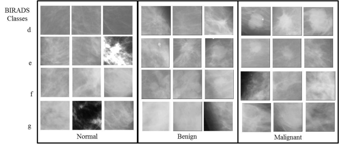
Figure 1: Samples of mammogram patches from the IRMA database. Row denotes the density of patches.

Some of the related works are summarized in Table 2, along with the details of feature vectors, classifiers, and a number of images used in experiments. The accuracy obtained for both types of classification (normal-abnormal and benign-malignant) is also given. The performance of approaches depends on different factors of mammogram patches such as dimension, number of training and testing samples, resolution and the type of abnormality. Most of the works in this area have tested on a subset of images instead of all mammogram patches, which we use.

Table 2: Summary of some related works on mammogram patch classification.

Feature	Classifier	Database	Number	Accuracy	Accuracy
			of images	(normal-abnormal)	(benign-malignant)
Gabor + PCA (Buciu & Gacsadi, 2011)	SVM	DDSM	NA	84.00%	78.00%
GLCM + DWT	BPNN∗	MIAS	332	98.10%	95.04%
(Beura et al., 2015)		DDSM	550	99.45%	97.61%
HOG, DSIFT, & LCP (Ergin & Kilinc, 2015)	SVM	DDSM	600	84.00%	78.00%
FFST	SVM	MIAS	228	98.29%	100.00%
(Gedik, 2016)		DDSM	228	100.00%	98.29%
Gabor	PSO∗∗+	DDSM	1024	98.82%	91.61%
(Khan et al., 2016)	SVM

^∗BPNN: Back Propagation Neural Network.
^∗∗PSO: Particle Swarm Optimization.

To summarize, in this work the two proposed feature extraction descriptors (HOT and PB-DCT with feature selection technique called Discrimination Potentiality) are compared with existing techniques for two-stage classification of all images of the IRMA database. This is done for individual density as well as together. We achieve higher accuracy than existing techniques for all images.

3 Proposed Mammogram Patch Classification System

This work proposes a two-stage mammogram patch classification system. In the first stage, mammogram patches are classified as normal-abnormal, and in the second stage, abnormal mammogram patches are classified as benign-malignant. The framework of the proposed work for training and testing phase is shown in Fig. 2.

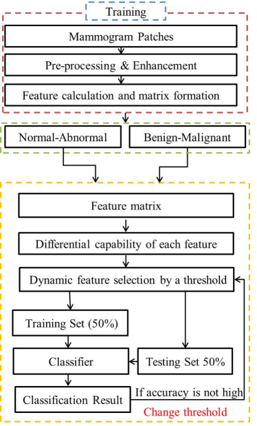
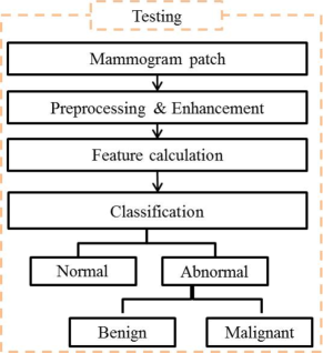
(a)	(b)

Figure 2: Flow diagram of the proposed mammogram patch classification system; (a) training phase and (b) testing phase.

Here, we first discuss image pre-processing and enhancement techniques used by us. Mammogram patches are preprocessed for illumination normalization and visibility enhancement of tumors and tissues (Anand & Gayathri, 2015; Sundaram et al., 2011). A two-stage adaptive histogram equalization enhancement technique is used here for texture enhancement of mammogram patches (Anand & Gayathri, 2015). Second, we discuss our two proposed feature extraction techniques, where features of mammogram patches are extracted from enhanced images. Finally, we discuss the feature selection technique used by us.

3.1 Pre-processing and Enhancement

In this work, for pre-processing, we only normalize the intensity of pixels and that too for a few mammogram patches. This is because while capturing images, illumination conditions are usually not the same. So, the range of the gray level is different for different mammogram patches. Hence, we use a simple and the most commonly used normalization formula (given below), which normalizes the intensity of pixels between 0 and 1 (Jain et al., 2005; Srisuk & Petpon, 2008).

$$I^{\prime}(x,y)=\frac{I(x,y)-\min(I)}{\max(I)-\min(I)},$$

where $(x,y)$ is the pixel position, $I^{\prime}(x,y)$ is the normalized pixel intensity, $I(x,y)$ is the actual pixel intensity, $\min(I)$ is the minimum intensity over all the pixels, and $\max(I)$ is the maximum intensity over all the pixels.

Next, we discuss tissue enhancement of mammogram patches. Histogram equalization is the one of the most basic technique here, which stretches the contrast of the high histogram regions and compresses the contrast of the low histogram regions. As a result, if the region of interest in an image occupies only a small portion, it will not be properly enhanced during histogram equalization.

This leads to more advanced techniques for enhancement, e.g., Adaptive Histogram Equalization (AHE), Contrast Limited Adaptive Histogram Equalization (CLAHE), Unsharp Masking (UM), Non-Linear Unsharp Masking (NLUM), Two-Stage Adaptive Histogram Equalization (TSAHE), etc (Anand & Gayathri, 2015; Panetta et al., 2011).

CLAHE has been found to be more suitable for tissue enhancement in mammogram patches. One aspect of enhancement is to capture the texture of the breast in mammogram patches better, which is defined by entropy. In the work of Anand & Gayathri (2015), authors have shown that TSAHE performs better than most of the existing techniques in not just the overall enhancement (defined by EME, i.e. Measure of Enhancement) but entropy as well.

Since cancerous cells mostly develop in tissues and our proposed descriptors (HOT and PB-DCT) are strongly tied to breast texture, we use a combination of CLAHE and TSAHE. We term it as TS-CLAHE.

We apply two stages of CLAHE on mammogram patches in a cascaded order. Firstly, histogram equalization is applied to $8\times 8$ sized blocks, followed by an application to $4\times 4$ sized of blocks. Fig. 3 shows the normalized and the enhanced image of a mammogram patch. It is observed that mass tissues are clearly visible in the enhanced image.

Figure 3: A preprocessed and enhanced mammogram patch.

3.2 Feature Extraction Techniques

As discussed in Sections 1 and 2, this work proposes two descriptors (HOT and PB-DCT) for mammogram patch classification. HOT is a modification of the HOG descriptor where a Gabor filter is used to calculate the angle and the magnitude response of texture of a mammogram patch. Selected PB-DCT coefficients based features are used here to improve the classification accuracy for each density class. Next, we discuss these two techniques separately. To the best of our knowledge, these strategies have not been applied anywhere for mammogram patch classification.

3.2.1 The Histogram of Oriented Texture (HOT) Descriptor

Here, we derive our HOT descriptor. Firstly, we discuss the calculations of gradient and orientation of an image as well as the HOG descriptor calculation from cells and blocks partitions (Ergin & Kilinc, 2015). Secondly, we describe a Gabor filter, which is used to extract magnitude and orientation of tissue texture information, and finally, we discuss modifications to the HOG descriptor that involves a Gabor filter and parameter selection.

Gradient of an image $I$ in horizontal and vertical directions, for a pixel position $(x,y)$ is computed as

$$dx = I(x+1,y)-I(x-1,y)\textrm{ and}$$

$$dy = I(x,y+1)-I(x,y-1),$$

respectively. For each pixel, $I(x,y)$, the gradient magnitude $m(x,y)$ and orientation $\theta(x,y)$ are computed as below.

$$m(x,y) = \sqrt{dx^{2}+dy^{2}}\textrm{ and}$$ (1)

$$\theta(x,y) = tan^{-1}\left(\frac{dy}{dx}\right).$$ (2)

Orientation range ($0^{0}-180^{0}$) is quantized into $B$ bins (i.e., $\theta(x,y)\in bin(b)$ with $b=1,2,3,\ldots,B$). The image is divided into $c\times c$ non-overlapping cells, and $l\times l$ cells are integrated as one block. Two adjacent blocks can overlap. The histogram of orientations ($HC(b)_{i}$) of bin$(b)$ within $i^{\textrm{th}}$ cell is computed as

$$HC(b)_{i} = HC(b)_{i}+m(x,y),$$

$$m(x,y) \in Cell_{i},$$

$$b = 1,2,3,\ldots,B,\ \text{and}$$

$$i = 1,2,3,\ldots,c\times c.$$

The histogram of $j^{\textrm{th}}$ block ($HB_{j}$) is obtained by integrating HCs (Histogram of Cells) within this block as follows:

$${HB}_{j} = HC_{1}\mathbin{\|}HC_{2}\mathbin{\|}\ldots\mathbin{\|}HC_{l\times l},$$

where $\mathbin{\|}$ denotes histograms concatenation into a vector. The vector of $HB_{j}$ is finally normalized by $L_{2}$-norm block normalization as below to obtain ${NHB}_{j}$.

$${NHB}_{j}=\frac{HB_{j}}{\sqrt{\|HB_{j}\|^{2}_{2}+e^{2}}},$$

where $e$ is a small constant to avoid problem of division by zero. Histogram of Oriented Gradients (HOG) can be obtained by integrating normalized histograms of all blocks as below.

$$HOG={NHB_{1}\mathbin{\|}NHB_{2}\mathbin{\|}\ldots NHB_{j}\mathbin{\|}\ldots,\mathbin{\|}NHB_{N}},$$

where $N$ is the number of possible blocks in an image, which is equal to $(c-l+1)\times(c-l+1)$. Fig. 4 shows an example of cell partitions, formation of overlapped blocks and concatenation of histograms to get the HOG descriptor. Finally, the length of HOG is $l^{2}\times{(c-l+1)}^{2}\times B$.

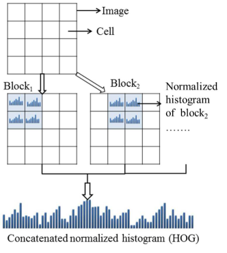
Figure 4: The HOG descriptor calculation.

Different line-shape filters or tools are available in the literature to extract lines and orientation features of a texture image (Khan et al., 2016). 2-D Gabor filters have been found more suitable filter bank to extract biological-like textural features of simple cells in the mammalian visual system (Kamarainen et al., 2006). Thus, a Gabor filter is ideal for calculating multi-orientation texture features of a mammogram patch. A Gabor function is defined as follows:

$$\begin{array}[]{lcr}G(x,y,\theta,\mu,\sigma)&=&\frac{1}{2\pi\sigma^{2}}\exp\left\{-\frac{x^{2}+y^{2}}{2\sigma^{2}}\right\}\exp\left[2\pi i\left(\mu x\cos\theta+\mu y\sin\theta\right)\right],\end{array}$$ (3)

where $i=\sqrt{-1}$, $\mu$ is the frequency of the sinusoidal wave, $\theta$ controls the orientation of the function, and $\sigma$ is the standard deviation of the Gaussian envelop. Based upon this Gabor function, a set of Gabor filters can be created for different scales and orientations.

Here, texture feature extraction for a given mammogram patch image ($I$) is calculated by the real part of a Gabor filter bank with eight different orientations and a fixed scale. Gabor magnitude, $m(x,y)_{Gabor}$, and Gabor orientation, $\theta(x,y)_{Gabor}$, response of each pixel $(x,y)$ are computed as

$$m_{Gabor}(x,y)=min(I(x,y)\ast G(x,y,\theta_{t},\mu,\sigma))\ \ \textrm{and}\\$$

$$\theta_{Gabor}(x,y)=argmin_{t}(I(x,y)\ast G(x,y,\theta_{t},\mu,\sigma)),$$

where $*$ means the convolution operation. The direction $\theta_{t}$ is calculated as follows:

$$\theta_{t}=\frac{\pi(t-1)}{8},\textrm{ }t=1,2,\ldots,8.$$

The features are calculated by varying the values of $\sigma$ and $\mu$. Fig. 5 shows the magnitude and angle image of a mammogram patch.

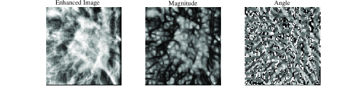
Figure 5: Gabor magnitude and angle image.

We combine HOG with a Gabor filter and name it as Histogram of Oriented Texture (HOT). HOT is computed in the same way as HOG, but $m_{Gabor}(x,y)$ and $\theta_{Gabor}(x,y)$ are used as magnitude and orientation of texture line instead of (1) and (2), respectively.

Finally, optimum parameters of the HOT descriptor, for both types of classification, are chosen by experiments. The value of $\sigma$ is varied from one to five to obtain an optimum number. The value of $\mu$ is computed as $\frac{1}{\sqrt{2\sigma}}$. In this work, the magnitude image is divided into equal sized $16\times 16$ cells. Size of a block considered is $2\times 2$, therefore, $15\times 15$ overlapped blocks are formed. The orientation range ($0^{0}-180^{0}$) is quantized into $8$ bins, and therefore, the final length of the resultant HOT descriptor is 7200. The length of the HOT descriptor is large, and all features do not have same discrimination capability (Liu et al., 2002). Feature selection schemes help to select more appropriate features. This is discussed in Section 3.3.

Next, we compare our proposed HOT descriptor with other works that use a combination of HOG and Gabor filter. In work by Xu et al. (2015), authors use a Gabor filter to extract features and HOG to reduce the dimension of the extracted feature vector. However, we use a combination of both to extract features. Comparison with two other works in this area is given in Table 3. Apart from the differences discussed until now, we (i.e. in the HOT descriptor) use Discrimination Potentiality for feature selection, which none of the other works use.

Table 3: Comparison of various descriptors using a combination of HOG and Gabor filter

Parameters	HoGG (Conde et al., 2013)	Gabor-HOG (Ouanan et al., 2015)	HOT
Number of Orientations	9	4	8
Number of Bins	9	9	8
Number of Cells to Divide Image	4 $\times$ 8	Rectangular Cells (Number Not Given)	16 $\times$ 16
Overlapped Image Area	3 $\times$ 7	Half of the Image	15 $\times$ 15
Feature Vector Length	756	81	7200
Application Area	Human Detection for Surveillance	Face Recognition	Mammogram Patch Classification

3.2.2 Pass Band - Discrete Cosine Transform (PB-DCT)

2D Discrete Cosine Transform (DCT) transforms images into frequency representation from the spatial form. It also provides energy compaction, that helps to reduce the information redundancy by retaining only a few coefficients. DCT coefficients of $I(x,y)$ image of $M\times N$ size are calculated as follows:

$$F(u,v) = \frac{1}{\sqrt{MN}}\alpha(u)\alpha(v)\sum_{x=0}^{M-1}\sum_{y=0}^{N-1}I(x,y)\times$$

$$\cos\left(\frac{(2x+1)u\pi}{2M}\right)\times cos\left(\frac{(2y+1)v\pi}{2N}\right)\textrm{ with}$$

$${\textrm{ }u=0,1,2,\ldots,M,\textrm{ }v=0,1,2,\ldots,N,}$$

where $\alpha(\omega)$ is defined by

$$\alpha(\omega)=\left\{\begin{array}[]{cc}\frac{1}{\sqrt{2}}&\omega=0\\ 1&\textrm{otherwise}.\end{array}\right.$$

DCT based various feature extraction and compression techniques have been proposed in literature (Dabbaghchian et al., 2010). Usually, DCT features are formed by selecting the most prominent and discriminating coefficients based upon some criterion (Dabbaghchian et al., 2010). The DCT coefficients can be divided into three sets, low frequencies, middle frequencies and high frequencies. Low frequencies are correlated with illumination conditions, middle frequencies represent texture features, while high frequencies represent small variance or noise. Illumination and texture properties are important for mammogram patch classification. Therefore, this work uses low and middle coefficients to form the descriptor (the Pass Band - Discrete Cosine descriptor or abbreviated as PB-DCT). Finally, the more discriminate DCT coefficients are selected based upon a discrimination criterion, which is discussed in the next section.

3.3 Feature Selection with Discrimination Potentiality

All features do not have the same ability to discriminate various classes (normal-abnormal and benign-malignant) (Liu et al., 2002), and they do not increase the accuracy based on available information for each class. Therefore, it is necessary to eliminate irrelevant features and select the most discriminative features among a given set of features (Kao et al., 2010). Determining features to improve accuracy as well as reduce searching time is a difficult task. As discussed in Section 2, feature subset selection techniques have been found to be more suitable for mammogram patch classification as compared to dimension reduction techniques.

There exist many techniques for feature selection. Some of the common ones are as follows: PCA (Principal Component Analysis) method, Markov blanket method, wrapper methods (e.g., sequential selection algorithm, genetic algorithms etc.), filter methods (e.g., Pearson correlation criteria, mutual information etc.), embedded methods, and statistical measures based methods (e.g., T-test, Kolmogorov-Smirnov test, Kullback-Leibler divergence etc.) (Chandrashekar & Sahin, 2014; Zeng et al., 2009).

Out of these, wrapper methods, filter methods, and statistical measures based methods are usually used for mammogram patch classification. Wrapper methods are computationally expensive since the number of steps required for obtaining the feature subset are very high. Filter methods sometimes lead to a redundant feature subset, and hence, are not optimal in this sense. (Chandrashekar & Sahin, 2014). Thus, we go for statistical measures based methods since they do not have the above discussed drawbacks. These methods also have the advantage in reducing the feature space without significantly degrading the classification performance (Dong & Wang, 2009).

The T-test method is one such method that gives a high score to features that capture the texture and the shape of mammograms (Nandi et al., 2006). As earlier, capturing texture is very important to us. Moreover, the T-test method is computationally light, easy to implement, and has been very recently successfully applied in mammogram context (Gedik, 2016; Jenifer et al., 2016). Thus, we use this feature selection method and show in the results section that this works very well with our proposed descriptors (DP-HOT and DP-PB-DCT). We term it as Discrimination Potentiality (DP) because of its capability in discriminating between the available features.

The discrimination potentiality $DP_{k}$ of the $k^{\textrm{th}}$ feature between two classes (a and b) is computed from a given training set as follows:

$$DP_{k}=\frac{\mu_{a,k}-\mu_{b,k}}{\sqrt{\frac{\delta_{a,k}^{2}}{n_{a}}-\frac{\delta_{b,k}^{2}}{n_{b}}}},$$

where $\mu_{a,k}$, $\mu_{b,k}$, and $\delta_{a,k}$, $\delta_{b,k}$, are mean and standard deviation values of the $k^{\textrm{th}}$ feature for $a$ and $b$ classes, respectively. $n_{a}$ and $n_{b}$ are the number of mammogram patches for $a$ and $b$ classes, respectively. A high value of DP means high discrimination ability of the corresponding feature (Jenifer et al., 2016).

All features (columns) of the feature matrix are arranged in descending order of their $DP$ value. Initially, first five features with highest $DP$ values are chosen for classification accuracy. Then, classification accuracy is calculated by adding features, with next higher value of $DP$, one by one until we get the highest accuracy. The optimum subset of features corresponding to the highest accuracy is selected as the final descriptor.

4 Experimental Results

Experiments are carried out in $\textrm{MATLAB}^{\textregistered}$ on a machine with Intel Quad Core processor @2.83GHz and 8GB RAM. As discussed earlier, mammogram patches are taken from the IRMA database (the MIAS and DDSM datasets). All images from this database (density wise), as given earlier in Table 1, are used. The size of each mammogram patch is $128\times 128$.

We first use two-fold cross validation, where the dataset is randomly divided into two equal parts. One part is used for training and the other is used for testing. Then, the two parts are swapped. That is, the one used for training earlier is now used for testing, and the one used for testing earlier is now used for training. At the end of this exercise, average performance is saved. Finally, we repeat two-fold cross validation ten times so as to remove any bias related to the division of the dataset.

The performance of our system (and comparative systems) is evaluated by standard metrics of sensitivity, specificity, accuracy and AUC (Area Under the ROC Curve).

Sensitivity is computed as the number of true positive cases over the number of actual positive cases. It is represented as follows:

$$Sensitivity=\frac{TP}{TP+FN}(\%),$$

where TP means True Positive cases and FN means False Negative cases.

Specificity is computed as the number of true negative cases over the number of actual negative cases. It is represented as follows:

$$Specificity=\frac{TN}{FP+TN}(\%),$$

where TN means True Negative cases and FP means False Positive cases.

Accuracy is computed as the number of correct classifications over the number of given cases. It is represented as follows:

$$Accuracy=\frac{TP+TN}{TP+FN+FP+TN}(\%).$$

AUC (Area Under the ROC Curve) provides a measure of the overall performance of the classifier, i.e. larger the area, better the classification. It is calculated from the trapezoidal rule as below (Yeh, 2002).

$$AUC=\frac{1}{2}\sum_{k=1}^{n}((Spec(k)-Spec(k+1))*(Sens(k)+Sens(k+1)))(\%),$$

where $n$ is the total number of test cases, and $Spec(k)$ and $Sens(k)$ are Specificity and Sensitivity for the $k^{th}$ test case, respectively. In the case of an ideal classification system, the value of all the four metrics should be close to 100%.

This section has three subparts. In Section 4.1, experiments related to finding the optimum parameters of the Histogram of Oriented Texture (HOT) descriptor with Discrimination Potentiality (DP), from now on referred as DP-HOT, are given. Similar experimental results for the Pass Band - Discrete Cosine Transform (PB-DCT) descriptor with Discrimination Potentiality (DP), from now on referred as DP-PB-DCT, are given in Section 4.2. Finally, in Section 4.3, the performance of both our proposed descriptors, DP-HOT and DP-PB-DCT, is compared with the performance of the existing (and popular) descriptors.

For fixing the parameters, only the training data is used ($i.e.$ 50%, as we use two-fold cross validation) and the validation data for testing is kept blind.

4.1 Performance of DP-HOT

Firstly, experiments are performed to find optimum parameters of Gabor filter for all the classes. Performance parameters are calculated by varying the value of $\sigma$ from one to five to obtain suitable scale for each density class. The best accuracy obtained by varying $\sigma$ is mentioned here.

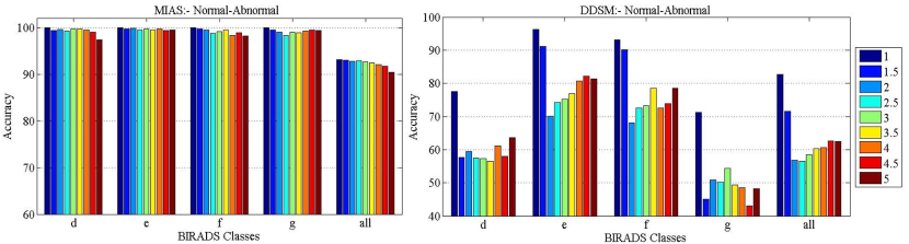
Figure 6: Comparison of normal-abnormal classification accuracies obtained by varying the value of $\sigma$ from one to five for each individual BIRADS class.

Fig. 6 compares normal-abnormal classification accuracy for different values of $\sigma$ for each class. It is observed that the DP-HOT descriptor achieves approximately 100% accuracy for all values of $\sigma$ for all the classes of the MIAS dataset. The maximum normal-abnormal classification accuracy of all the classes combined is achieved with $\sigma$ as one. It is difficult to infer the optimum value of $\sigma$ by observing the bar chart of the MIAS dataset only. In case of the DDSM dataset, the DP-HOT descriptor with $\sigma$ as one gives the best accuracy for all the classes individually as well as combined. For classes $e$ and $f$, DP-HOT achieves an accuracy of around 95%, while it does not achieve good accuracy for classes $d$ and $g$ (around 70%).

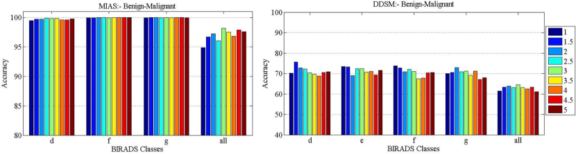
Figure 7: Comparison of benign-malignant classification accuracies obtained by varying the value of $\sigma$ from one to five for each individual BIRADS class.

Fig. 7 compares benign-malignant classification accuracy for different values of $\sigma$ for each class. The DP-HOT descriptor again achieves approximately 100% accuracy for all values of $\sigma$ for all the classes of the MIAS dataset. The maximum benign-malignant classification accuracy for all the classes combined is achieved with $\sigma$ as 3. For the DDSM dataset, the DP-HOT descriptor performs equally for all $\sigma$ for all the classes (around 70%).

First observation is that DP-HOT does not perform very well for both types of classification (normal-abnormal and benign-malignant) for the DDSM dataset (although it does perform well for MIAS). The reason, as discussed in Section 2, is that texture information plays a big role in both types of classifications (normal-abnormal and benign-malignant), and DP-HOT does not capture that well for the DDSM dataset. The DP-PB-DCT descriptor overcomes this drawback to a great extent. Another observation is that classification accuracy for an individual class is better than combined. This is intuitive since images in a class are similar.

Table 4 lists the feature length used for both types of classification (normal-abnormal and benign-malignant) done on both the datasets (MIAS and DDSM) for each density class.

Table 4: Feature length for the DP-HOT descriptor.

BIRADS Class	MIAS: Feature Length	DDSM: Feature Length
Normal-Abnormal
$d$	2655	210
$e$	10	100
$f$	30	75
$g$	20	200
All	40	140
Benign-Malignant
$d$	2000	225
$e$	All Benign	130
$f$	2000	405
$g$	1790	170
All	2000	990

4.2 Performance of DP-PB-DCT

As in the case of the DP-HOT descriptor, in Table 5 we list the feature length used for both types of classification (normal-abnormal and benign-malignant) done on both the datasets (MIAS and DDSM) for each density class when using the DP-PB-DCT descriptor.

Table 5: Feature length for the DP-PB-DCT descriptor.

BIRADS Class	MIAS: Feature Length	DDSM: Feature Length
Normal-Abnormal
$d$	5	4000
$e$	5	4000
$f$	5	995
$g$	5	1315
All	5	430
Benign-Malignant
$d$	5	4350
$e$	5	4005
$f$	5	3995
$g$	5	4625
All	5	5065

Since, the selection of features in the DP-PB-DCT descriptor is more critical, we do further feature selection analysis here. Fig. 8 compares accuracy against the number of features for normal-abnormal and benign-malignant classification for each density class separately and combined. As in the case of DP-HOT, the performance for individual density is better than combined. Moreover, multiple points with the high classification accuracy are observed.

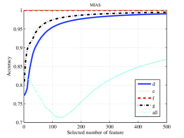
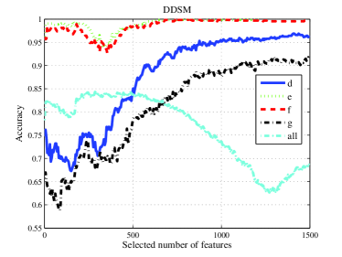
(MIAS)	(DDSM)
Normal-Abnormal
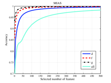
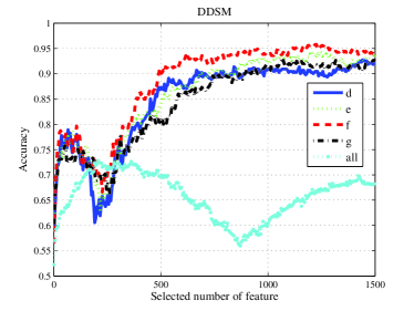
(MIAS)	(DDSM)
Benign-Malignant

Figure 8: Performance accuracy against the number of DP-PB-DCT features.

4.3 Comparison with Other Techniques

The performance of the two proposed descriptors is compared with some related descriptors such as Zernike moment (Tahmasbi et al., 2011), MLPQ (Nanni et al., 2012), GRsca (Nanni et al., 2013), WGLCM (Beura et al., 2015), LCP (Ergin & Kilinc, 2015) and HOG (Ergin & Kilinc, 2015) for each density class separately as well as combined. The performance of each descriptor is evaluated in the same experimental setup including the use of the same testing protocol.

The parameters of each of these descriptors are selected as given in the literature to achieve the best performance for mammogram patch classification. These parameters are summarized below.

The Zernike moment descriptor is computed by dividing a mammogram patch into $4\times 4$ blocks. $120$ Zernike moments are used for obtaining the final mammogram patch descriptor. Therefore, the length of the feature vector is $4\times 4\times 120$ (Tahmasbi et al., 2011).

The MLPQ descriptor is computed by concatenating different Local Phase Quantization (LPQ) descriptors. Each LPQ descriptor is obtained by varying values of three different parameters. This includes filter size ($r$ with values $1,3,5$), the scalar frequency ($a$ with values $0.8,1.0,1.2,1.4,1.6$), and the correlation coefficient ($\rho$ with values $0.75,0.95,1.15,1.35,1.55,1.75,1.95$). Each LPQ descriptor’s length is standard ($256$). Therefore, the length of the feature vector is $3\times 5\times 7\times 256$ (Nanni et al., 2012).

The GRsca descriptor extracts features from the three gray-level run length co-occurrence matrices corresponding to the original image and two filtered images (using a filter of size $3$ and $5$). These images are divided into four blocks. Features are obtained from co-occurrence matrix and these four blocks. A set of ten different descriptors is calculated at four different orientations and two different distances. Therefore, the length of the feature vector is $3\times 5\times 10\times 4\times 2$ (Nanni et al., 2013).

The Wavelet Gray Level Co-occurrence Matrix (WGLCM) descriptor is computed by decomposing the image into one approximation. Detail coefficients up to two levels with a wavelet filter are used. For each level, three decompositions (along horizontal, vertical and diagonal directions) are obtained. The normalized GLCM (NGLCM) matrices of all detail coefficients are calculated in four directions ($0^{\circ}$, $45^{\circ}$, $90^{\circ}$, and $135^{\circ}$) with a single displacement. Contrast, homogeneity, energy, and correlation statistical properties of all NGLCM matrices are calculated and concatenated into a vector. Therefore, the length of the feature vector is $2\times 3\times 4\times 4$ (Beura et al., 2015).

Local Configure Pattern (LCP) is a modification of Local Binary Pattern (LBP). Here, first, the weights associated with intensities of neighboring pixels are used to linearly reconstruct the central pixel intensity. Then, the error between the central pixel and its neighbor is minimized. In this work, LCP images are computed for radius $1$ to $5$. Each LCP image is divided into $4\times 4$ blocks. The histogram of each block is concatenated with $58$ bins, and the result is used as a mammogram patch descriptor. Therefore, the length of the feature vector is $5\times 4\times 4\times 58$ (Ergin & Kilinc, 2015).

Histogram of Gradients (HOG) is calculated using $16\times 16$ cell partitions. The size of the block considered is $2\times 2$, thus, $15\times 15$ overlapped blocks are formed. The orientation range is quantized into $8$ bins. Therefore, the length of the feature vector is $2\times 2\times 15\times 15\times 8$ (Ergin & Kilinc, 2015).

The optimum parameters of DP-HOT and DP-PB-DCT are selected based upon experiments as discussed in the previous subsections. The length of each descriptor is different and the appropriate feature set for each descriptor is selected based upon the DP values as described earlier.

4.3.1 Classification Results

Table 6 compares sensitivity, specificity, accuracy and AUC for normal-abnormal classification with all the above descriptors on the MIAS and DDSM datasets. The performance parameters for all the descriptors are provided for each density class separately as well as combined. The best performing systems are highlighted in bold.

Table 6: Mammogram patch classification results as normal-abnormal for the MIAS and DDSM datasets.

Descriptor	BIRADS	MIAS				DDSM
		Sens.	Spec.	Acc.	AUC	Sens.	Spec.	Acc.	AUC
Zernike (Tahmasbi et al., 2011)	$d$	99.12	93.59	97.32	90.28	90.01	68.64	83.32	91.69
	$e$	94.98	99.63	98.81	100	99.78	85.12	95.86	100
	$f$	92.86	99.88	97.29	100	99.56	95.91	98.46	100
	$g$	91.31	97.87	95.42	75.82	83.32	36.72	68.63	81.89
	All	75.92	91.70	85.39	85.11	91.90	61.99	82.95	82.03
MLPQ (Nanni et al., 2012)	$d$	89.21	75.00	84.70	90.28	80.29	73.51	78.16	89.71
	$e$	100	96.30	96.96	100	99.97	99.97	99.97	100
	$f$	100	100	100	100	99.91	99.91	99.91	100
	$g$	68.75	92.31	83.10	90.66	83.14	54.06	73.97	81.80
	All	72.60	88.50	82.14	88.15	86.07	88.14	86.69	93.59
GRsca (Nanni et al., 2013)	$d$	76.92	70.00	74.59	85.90	86.03	79.53	84.00	88.23
	$e$	100	100	100	100	100	100	100	100
	$f$	100	100	100	100	100	100	100	100
	$g$	66.96	100	87.86	84.13	83.41	63.85	77.24	82.26
	All	68.95	98.79	86.85	91.26	88.44	88.64	88.50	95.48
WGLCM (Beura et al., 2015)	$d$	92.15	50.83	78.71	73.61	85.54	84.92	85.34	94.38
	$e$	90.91	100	98.40	100	99.84	99.98	99.87	100
	$f$	100	100	100	100	99.70	100	99.79	100
	$g$	60.96	100	85.93	80.77	84.94	62.25	77.78	85.81
	All	64.72	100	85.89	93.41	86.24	93.21	88.33	94.97
LCP (Ergin & Kilinc, 2015)	$d$	92.31	66.67	83.63	80.56	87.99	89.07	88.32	90.39
	$e$	100	100	100	100	100	100	100	100
	$f$	100	100	100	100	100	100	100	100
	$g$	73.21	96.15	87.74	64.42	86	69.10	80.67	74.93
	All	75	97.78	88.67	85.70	87.80	93.39	89.47	92.88
HOG (Ergin & Kilinc, 2015)	$d$	88.46	91.67	89.47	100	84.36	78.62	82.56	87.58
	$e$	100	100	100	100	99.57	94.64	98.25	98.79
	$f$	100	95.83	97.36	100	98.23	88.73	95.36	97.67
	$g$	85.71	100	95	100	82.22	56.52	74.12	77.70
	All	70	87.78	80.67	85.85	87.69	77.95	84.77	88.32
DP-HOT	$d$	100	100	100	100	83.44	64.69	77.57	91.20
	$e$	100	100	100	100	96.96	95.24	96.50	100
	$f$	100	100	100	100	94.69	89.75	93.20	100
	$g$	100	100	100	100	77.78	57.06	71.24	76.05
	All	87	98	93	97.26	84.80	77.30	82.56	86.21
DP-PB-DCT	$d$	100	100	100	100	98.19	94.01	96.88	98.39
	$e$	100	100	100	100	100	100	100	100
	$f$	100	100	100	100	100	100	100	100
	$g$	100	100	100	100	97.78	80.70	92.39	98.68
	All	97.18	98.89	97.33	100	87.18	79.37	84.84	92.20

Table 7: Mammogram patch classification results as benign-malignant for the MIAS and DDSM datasets.

Descriptor	BIRADS	MIAS				DDSM
		Sens.	Spec.	Acc.	AUC	Sens.	Spec.	Acc.	AUC
Zernike (Tahmasbi et al., 2011)	$d$	93.23	97.05	95.39	54.76	60.36	54.34	57.37	56.78
	$e$	-	-	-	-	60.09	60.34	60.22	58.39
	$f$	97.26	99.83	98.73	100	58.62	56.02	57.30	63.26
	$g$	95.61	98.96	97.62	100	57.96	70.98	64.44	57.22
	All	80.47	84.15	82.44	72.77	56.92	55.11	56.02	53.87
MLPQ (Nanni et al., 2012)	$d$	71.43	75.00	71.79	96.43	59.59	57.43	58.50	62.70
	$e$	-	-	-	-	61.72	59.36	60.55	63.24
	$f$	96.43	97.62	96.94	100	49.79	64.76	57.31	59.18
	$g$	100	83.33	93.75	93.34	95.98	17.70	56.67	57.66
	All	73.96	76.19	75.00	86.16	57.40	54.62	56.01	56.04
GRsca (Nanni et al., 2013)	$d$	64.29	58.33	60.26	62.86	66.83	54.21	60.47	62.01
	$e$	-	-	-	-	71.09	53.94	52.59	66.24
	$f$	85.71	28.57	61.22	58.34	63.59	56.54	60.05	64.32
	$g$	77.59	58.28	69.49	50	81.70	40.27	60.89	64.58
	All	96.88	35.71	68.33	68.75	67.69	52.63	60.15	64.21
WGLCM (Beura et al., 2015)	$d$	35.83	92.86	67.95	80.95	53.15	62.99	58.04	60.35
	$e$	-	-	-	-	50.88	63.79	57.39	56.32
	$f$	45.83	90.63	71.43	91.67	59.92	52.01	55.97	59.24
	$g$	47.22	86.25	70.83	93.34	57.08	60.71	58.89	57.59
	All	53.81	74.72	64.96	70.09	53.20	56.98	55.09	56.59
LCP (Ergin & Kilinc, 2015)	$d$	99.72	99.84	99.77	100	51.80	66.66	59.18	63.38
	$e$	-	-	-	-	57.89	62.93	60.43	60.86
	$f$	100	99.9	99.98	100	51.96	62.24	57.08	60.33
	$g$	99.99	99.96	99.98	100	56.64	61.16	58.89	60.04
	All	98.94	95.57	97.37	72.32	55.26	59.33	57.29	57.38
HOG (Ergin & Kilinc, 2015)	$d$	100	100	100	95.24	64.86	65.30	65.08	66.27
	$e$	-	-	-	-	59.65	65.52	62.61	70.01
	$f$	100	100	100	100	66.95	65.32	66.14	67.92
	$g$	100	100	100	100	63.27	66.07	64.67	68.07
	All	80.67	92.86	87.5	94.20	54.93	61.89	58.40	65.06
DP-HOT	$d$	100	100	100	100	72.07	68.49	70.29	80.44
	$e$	-	-	-	-	70.18	75	72.61	74.92
	$f$	100	100	100	100	72.66	69.31	71.02	83.91
	$g$	100	100	100	100	73.45	68.75	71.11	81.09
	All	98.83	97.57	98.24	100	64.56	64.67	64.61	68.89
DP-PB-DCT	$d$	100	100	100	100	96.85	94.53	95.69	98.13
	$e$	-	-	-	-	96.05	93.53	94.78	98.78
	$f$	100	100	100	100	97.35	96.45	96.90	98.87
	$g$	100	100	100	100	91.59	95.98	93.78	99
	All	100	100	100	100	73.53	71.33	72.43	82.93

For the MIAS dataset, both the proposed descriptors (DP-HOT and DP-PB-HOT) achieve near 100% sensitivity, specificity, accuracy, and AUC for all the classes. This is better than the six standard descriptors (Zernike moment, MLPQ, GRsca, WGLCM, LCP, and HOG).

For the DDSM dataset, although our DP-HOT descriptor performs almost as badly as the other six descriptors for all the classes (as low as around 65% for one performance parameter), DP-PB-DCT performs extremely well for all the classes (more than 92% for most performance parameters), which is better than the six standard descriptors. All the eight descriptors (the six standard and the two new) perform well for classes $e$ and $f$ but have a dip in the performance for classes $d$ and $g$. This is because for the DDSM dataset, texture discrimination for $e$ and $f$ classes is better than for $d$ and $g$ classes, which is crucial in normal-abnormal classification.

Table 7 compares performance parameters for benign-malignant classification with all the above eight descriptors for all the classes (and combined) of the MIAS and DDSM datasets. As earlier, the best performing systems are highlighted in bold. The results are similar to those for normal-abnormal classification. Note that in the MIAS dataset, the $e$ class has all benign images, so, classification was not performed for this. The corresponding rows in this table are left empty.

For the MIAS dataset, both the proposed descriptors (DP-HOT and DP-PB-DCT) perform slightly better than the six standard descriptors for all the classes (achieve near 100% sensitivity, specificity, accuracy, and AUC).

For the DDSM dataset, DP-HOT is slightly better than the existing descriptors (around 70% for all performance parameters), while DP-PB-DCT is much better than the six standard descriptors for all the classes (more than 92% for most performance parameters).

To summarize, as mentioned in Section 2 as well as Section 4.1, capturing texture information is of utmost importance for mammogram patch classification (both normal-abnormal and benign-malignant). In general, DP-HOT captures this texture information slightly better than the six standard descriptors, and hence, it performs slightly better than these. DP-PB-DCT captures texture information best, and hence, performs much better than all the others.

5 Conclusion and Future Work

We propose a variant of HOG and Gabor filter combination, which we call Histogram of Oriented Texture (HOT) for mammogram patch classification. We also revisit the Pass Band - Discrete Cosine Transform (PB-DCT) descriptor for the same. The feature selection technique of Discrimination Potentiality (DP) is used with the above two descriptors for mammogram patch classification. This results in two new descriptors (DP-HOT and DP-PB-DCT). We consider the density of mammogram patches as a factor for classification (this was not done earlier), and show that this plays an important role in classification.

Our two-stage patch classification system (normal-abnormal and benign-malignant), using the two new descriptors for each density class, is tested on all images of the MIAS and DDSM datasets from the IRMA repository (in literature, experiments have been done only on a subset of these images). We achieve a high classification performance (in terms of specificity, sensitivity, accuracy and AUC) in an absolute sense as well as in relative sense (compared with the six standard descriptors). This is due to the fact that textural information in a mammogram patch is crucial for classification, and our descriptors capture that well.

Future work here involves developing a Computer-Aided Diagnosis (CAD) application for full mammogram using our framework. This will aid radiologists for more accurate diagnosis of breast cancer using only the information about mammogram density.

6 Acknowledgment

The authors would like to thank Prof. Dr.rer.nat. Dipl.-Ing. Thomas Martin Deserno, Department of Medical Information, Division of Image and Data Management, RWTH Aachen, Germany, for providing us the images.

Thanks to the anonymous reviewers that helped to greatly improve the quality of this manuscript. We would also like to thank the editor handling our manuscript, Prof. Binshan Lin (at Louisiana State University, Shreveport), in giving us the flexibility during revision submissions.

References

References

- Abdel-Nasser et al. (2015) Abdel-Nasser, M., Rashwan, H. A., Puig, D., & Moreno, A. (2015). Analysis of tissue abnormality and breast density in mammographic images using a uniform local directional pattern. Expert Systems with Applications, 42, 9499–9511.
- Anand & Gayathri (2015) Anand, S., & Gayathri, S. (2015). Mammogram image enhancement by two-stage adaptive histogram equalization. Optik-International Journal for Light and Electron Optics, 126, 3150–3152.
- Beura et al. (2015) Beura, S., Majhi, B., & Dash, R. (2015). Mammogram classification using two dimensional discrete wavelet transform and gray-level co-occurrence matrix for detection of breast cancer. Neurocomputing, 154, 1–14.
- Buciu & Gacsadi (2011) Buciu, I., & Gacsadi, A. (2011). Directional features for automatic tumor classification of mammogram images. Biomedical Signal Processing and Control, 6, 370–378.
- Chandrashekar & Sahin (2014) Chandrashekar, G., & Sahin, F. (2014). A survey on feature selection methods. Computers & Electrical Engineering, 40, 16–28.
- Conde et al. (2013) Conde, C., Moctezuma, D., De Diego, I. M., & Cabello, E. (2013). HoGG: Gabor and HoG-based human detection for surveillance in non-controlled environments. Neurocomputing, 100, 19–30.
- Dabbaghchian et al. (2010) Dabbaghchian, S., Ghaemmaghami, M. P., & Aghagolzadeh, A. (2010). Feature extraction using discrete cosine transform and discrimination power analysis with a face recognition technology. Pattern Recognition, 43, 1431–1440.
- De Oliveira et al. (2011) De Oliveira, J. E. E., De Albuquerque Araújo, A., & Deserno, T. M. (2011). Content-based image retrieval applied to BIRADS tissue classification in screening mammography. World journal of radiology, 3, 24–31.
- De Oliveira et al. (2008) De Oliveira, J. E. E., Deserno, T. M., & De Albuquerque Araújo, A. (2008). Breast lesions classification applied to a reference database. In Proceedings of the 2nd International Conference on E-Medical Systems (pp. 29–31). SETIT.
- Deserno (2012) Deserno, T. M. (2012). IRMA database. http://ganymed.imib.rwth-aachen.de/deserno/datasets_en.php?SELECTED=00014#00014.dataset. Accessed: 1-03-2016.
- Deserno et al. (2012) Deserno, T. M., Soiron, M., & De Oliveira, J. E. E. (2012). Texture patterns extracted from digitizes mammograms of different BI-RADS classes. Image Retrieval in Medical Applications project, 1.
- Dong & Wang (2009) Dong, A., & Wang, B. (2009). Feature selection and analysis on mammogram classification. In Proceedings of the IEEE Pacific Rim Conference on Communications, Computers and Signal Processing (pp. 731–735). IEEE.
- Ergin & Kilinc (2015) Ergin, S., & Kilinc, O. (2015). A new feature extraction framework based on wavelets for breast cancer diagnosis. Computers in Biology and Medicine, 51, 171–182.
- Gedik (2016) Gedik, N. (2016). A new feature extraction method based on multi-resolution representations of mammograms. Applied Soft Computing, 44, 128–133.
- Jain et al. (2005) Jain, A., Nandakumar, K., & Ross, A. (2005). Score normalization in multimodal biometric systems. Pattern recognition, 38, 2270–2285.
- Jenifer et al. (2016) Jenifer, S., Parasuraman, S., & Kadirvelu, A. (2016). Contrast enhancement and brightness preserving of digital mammograms using fuzzy clipped contrast-limited adaptive. Applied Soft Computing, 42, 167–177.
- Kamarainen et al. (2006) Kamarainen, J. K., Kyrki, V., & Kälviäinen, H. (2006). Invariance properties of Gabor filter-based features - Overview and applications. IEEE Transactions on Image Processing, 15, 1088–1099.
- Kao et al. (2010) Kao, W. C., Hsu, M. C., & Yang, Y. Y. (2010). Local contrast enhancement and adaptive feature extraction for illumination-invariant face recognition. Pattern Recognition, 43, 1736–1747.
- Khan et al. (2016) Khan, S., Hussain, M., Aboalsamh, H., Mathkour, H., Bebis, G., & Zakariah, M. (2016). Optimized Gabor features for mass classification in mammography. Applied Soft Computing, 44, 267–280.
- Laadjel et al. (2015) Laadjel, M., Al-Maadeed, S., & Bouridane, A. (2015). Combining Fisher locality preserving projections and passband DCT for efficient palmprint recognition. Neurocomputing, 152, 179–189.
- Leena Jasmine et al. (2009) Leena Jasmine, J. S., Govardhan, A., & Baskaran, S. (2009). Microcalcification detection in digital mammograms based on wavelet analysis and neural networks. In Proceedings of the IEEE International Conference on Control, Automation, Communication and Energy Conservation (pp. 1–6). IEEE.
- Liu et al. (2002) Liu, H., Li, J., & Wong, L. (2002). A comparative study on feature selection and classification methods using gene expression profiles and proteomic patterns. Genome Informatics, 13, 51–60.
- Mudigonda et al. (2000) Mudigonda, N. R., Rangayyan, R. M., & Desautels, J. E. L. (2000). Gradient and texture analysis for the classification of mammographic masses. IEEE Transactions on Medical Imaging, 19, 1032–1043.
- Mudigonda et al. (2001) Mudigonda, N. R., Rangayyan, R. M., & Desautels, J. E. L. (2001). Detection of breast masses in mammograms by density slicing and texture flow-field analysis. IEEE Transactions on Medical Imaging, 20, 1215–1227.
- Muramatsu et al. (2016) Muramatsu, C., Hara, T., Endo, T., & Fujita, H. (2016). Breast mass classification on mammograms using radial local ternary patterns. Computers in Biology and Medicine, 72, 43–53.
- Nandi et al. (2006) Nandi, R. J., Nandi, A. K., Rangayyan, R. M., & Scutt, D. (2006). Genetic programming and feature selection for classification of breast masses in mammograms. In Proceedings of the 28th IEEE Annual International Conference on Engineering in Medicine and Biology Society (pp. 3021–3024). IEEE.
- Nanni et al. (2013) Nanni, L., Brahnam, S., Ghidoni, S., Menegatti, E., & Barrier, T. (2013). Different approaches for extracting information from the co-occurrence matrix. PLOS ONE, 8, e83554.
- Nanni et al. (2012) Nanni, L., Brahnam, S., & Lumini, A. (2012). A very high performing system to discriminate tissues in mammograms as benign and malignant. Expert Systems with Applications, 39, 1968–1971.
- Ojala et al. (2002) Ojala, T., Pietikainen, M., & Maenpaa, T. (2002). Multiresolution gray-scale and rotation invariant texture classification with local binary patterns. IEEE Transactions on Pattern Analysis and Machine Intelligence, 24, 971–987.
- Ojansivu & Heikkilä (2008) Ojansivu, V., & Heikkilä, J. (2008). Blur insensitive texture classification using local phase quantization. In Proceedings of the International Conference on Image and Signal Processing (pp. 236–243). Springer.
- Oliver et al. (2010) Oliver, A., Freixenet, J., Martí, J., Pérez, E., Pont, J., Denton, E. R. E., & Zwiggelaar, R. (2010). A review of automatic mass detection and segmentation in mammographic images. Medical Image Analysis, 14, 87–110.
- Oliver et al. (2008) Oliver, A., Freixenet, J., Martí, R., Pont, J., Pérez, E., Denton, E. R. E., & Zwiggelaar, R. (2008). A novel breast tissue density classification methodology. IEEE Transactions on Information Technology in Biomedicine, 12, 55–65.
- Oliver et al. (2007) Oliver, A., Lladó, X., Freixenet, J., & Martí, J. (2007). False positive reduction in mammographic mass detection using local binary patterns. In Proceedings of the 10th Springer International Conference on Medical Image Computing and Computer-assisted Intervention (pp. 286–293). Springer.
- Oliver et al. (2012) Oliver, A., Torrent, A., Lladó, X., Tortajada, M., Tortajada, L., Sentís, M., Freixenet, J., & Zwiggelaar, R. (2012). Automatic microcalcification and cluster detection for digital and digitised mammograms. Knowledge-Based Systems, 28, 68–75.
- Ouanan et al. (2015) Ouanan, H., Ouanan, M., & Aksasse, B. (2015). Gabor-HOG features based face recognition scheme. Indonesian Journal of Electrical Engineering and Computer Science, 15, 331–335.
- Panetta et al. (2011) Panetta, K., Zhou, Y., Agaian, S., & Jia, H. (2011). Nonlinear unsharp masking for mammogram enhancement. IEEE Transactions on Information Technology in Biomedicine, 15, 918–928.
- Peng et al. (2016) Peng, W., Mayorga, R. V., & Hussein, E. M. A. (2016). An automated confirmatory system for analysis of mammograms. Computer Methods and Programs in Biomedicine, 125, 134–144.
- Petroudi & Brady (2011) Petroudi, S., & Brady, M. (2011). Breast density characterization using texton distributions. In Proceedings of the 33rd IEEE International Conference on Engineering in Medicine and Biology Society (pp. 5004–5007). IEEE.
- Rabottino et al. (2008) Rabottino, G., Mencattini, A., Salmeri, M., Caselli, F., & Lojacono, R. (2008). Mass contour extraction in mammographic images for breast cancer identification. In Proceedings of the 16th IMEKO TC4 Symposium - Exploring New Frontiers of Instrumentation and Methods for Electrical and Electronic Measurements.
- Rangayyan et al. (2007) Rangayyan, R. M., Ayres, F. J., & Desautels, J. E. L. (2007). A review of computer-aided diagnosis of breast cancer: Toward the detection of subtle signs. Journal of the Franklin Institute, 344, 312–348.
- Rouhi et al. (2015) Rouhi, R., Jafari, M., Kasaei, S., & Keshavarzian, P. (2015). Benign and malignant breast tumors classification based on region growing and CNN segmentation. Expert Systems with Applications, 42, 990–1002.
- Shah (2016) Shah, S. (2016). Statistics of breast cancer in India. http://www.breastcancerindia.net/statistics/stat_global.html. Accessed: 1-03-2016.
- Shanthi & Murali Bhaskaran (2012) Shanthi, S., & Murali Bhaskaran, V. (2012). Computer aided detection and classification of mammogram using self-adaptive resource allocation network classifier. In Proceedings of the IEEE International Conference on Pattern Recognition, Informatics and Medical Engineering (pp. 284–289). IEEE.
- Srisuk & Petpon (2008) Srisuk, S., & Petpon, A. (2008). A Gabor quotient image for face recognition under varying illumination. In Proceedings of the 4th International Symposium Visual Computing (Advances in Visual Computing) (pp. 511–520). Springer.
- Sundaram et al. (2011) Sundaram, M., Ramar, K., Arumugam, N., & Prabin, G. (2011). Histogram modified local contrast enhancement for mammogram images. Applied Soft Computing, 11, 5809–5816.
- Tahmasbi et al. (2011) Tahmasbi, A., Saki, F., & Shokouhi, S. B. (2011). Classification of benign and malignant masses based on Zernike moments. Computers in Biology and Medicine, 41, 726–735.
- Wajid & Hussain (2015) Wajid, S. K., & Hussain, A. (2015). Local energy-based shape histogram feature extraction technique for breast cancer diagnosis. Expert Systems with Applications, 42, 6990–6999.
- Xu et al. (2015) Xu, X., Quan, C., & Ren, F. (2015). Facial expression recognition based on Gabor Wavelet transform and Histogram of Oriented Gradients. In Proceedings of the IEEE International Conference on Mechatronics and Automation (pp. 2117–2122). IEEE.
- Yeh (2002) Yeh, S. T. (2002). Using trapezoidal rule for the area under a curve calculation. In Proceedings of the 27th Annual SAS® User Group International.
- Zeng et al. (2009) Zeng, Y., Luo, J., & Lin, S. (2009). Classification using Markov blanket for feature selection. In Proceedings of the IEEE International Conference on Granular Computing (pp. 743–747). IEEE.