Analytical coupled-channels treatment of two-body scattering in the presence of three-dimensional isotropic spin-orbit coupling

Abstract

It is shown that the single-particle spin-orbit coupling terms, which—in the cold atom context—are associated with synthetic gauge fields, can significantly and non-trivially modify the phase accumulation at small interparticle distances even if the length scale $(k_{\text{so}})^{-1}$ associated with the spin-orbit coupling term is significantly larger than the van der Waals length $r_{\text{vdW}}$ that characterizes the two-body interaction potential. A theoretical framework, which utilizes a generalized local frame transformation and accounts for the phase accumulation analytically, is developed. Comparison with numerical coupled-channels calculations demonstrates that the phase accumulation can, to a very good approximation, be described over a wide range of energies by the free-space scattering phase shifts—evaluated at a scattering energy that depends on $k_{\text{so}}$—and the spin-orbit coupling strength $k_{\text{so}}$.

The tunability of low-energy scattering parameters such as the $s$-wave scattering length $a_{s}$ and $p$-wave scattering volume $V_{p}$ by means of application of an external magnetic field in the vicinity of a Feshbach resonance chin has transformed the field of ultracold atom physics, providing experimentalists with a knob to “dial in” the desired Hamiltonian. This tunability has afforded the investigation of a host of new phenomena including the BEC-BCS crossover block_rev ; stringari_rev . Most theoretical treatments of these phenomena are formulated in terms of a few scattering quantities such as $a_{s}$ and $V_{p}$, which properly describe the low-energy behavior of the two-body system.

The recent realization of spin-orbit coupled cold atom systems spielman is considered another milestone, opening the door for the observation of topological properties and providing a new platform with which to study scenarios typically encountered in condensed matter systems with unprecedented control review_hui ; review_coloquium ; review_spielman . An assumption that underlies most theoretical treatments of cold atom systems with synthetic gauge fields is that the spin-orbit coupling term, i.e., the Raman laser that couples the different internal states or the shaking of the lattice that couples different bands, leaves the atom-atom interactions “untouched”. More specifically, mean-field treatments “simply” add the single-particle spin-orbit coupling term to the mean-field Hamiltonian and parameterize the atom-atom interactions via contact potentials with coupling strengths that are calculated for the two-body van der Waals potential without the spin-orbit coupling terms review_hui ; review_hui2 .

Consistent with such mean-field approaches, most two-body scattering studies derive observables based on the assumption that the two-body Bethe-Peierls boundary condition, derived in the absence of single-particle spin-orbit coupling terms, remains unaffected by the spin-orbit coupling terms, provided an appropriate “basis transformation” is accounted for pengzhang1 ; pengzhang2 ; xiaoling ; chris ; zhenhua1 ; guan ; quasi-1D ; gao . The underlying premise of these two-body and mean-field treatments is rooted in scale separation, which suggests that the free-space scattering length $a_{s}$ and scattering volume $V_{p}$ remain good quantities provided $(k_{\text{so}})^{-1}$ is larger than the two-body van der Waals length $r_{\text{vdW}}$. Indeed, model calculations for a square-well potential in the presence of three-dimensional isotropic spin-orbit coupling suggest that the above reasoning holds, provided $1/a_{s}$ and $V_{p}$ are small zhenhua2 .

This work revisits the question of how to obtain and parameterize two-body scattering observables in the presence of three-dimensional isotropic spin-orbit coupling. Contrary to what has been reported in the literature, our calculations for Lennard-Jones and square-well potentials show that the three-dimensional isotropic spin-orbit coupling terms can impact the phase accumulation in the small interparticle distance region where the two-body interaction potential cannot be neglected even if $(k_{\text{so}})^{-1}$ is notably larger than $r_{\text{vdW}}$. We observe non-perturbative changes of the scattering observables when $k_{\text{so}}$ changes by a small amount. An analytical treatment, which reproduces the full coupled-channels results such as the energy-dependent two-body cross sections for the finite-range potentials with high accuracy, is developed. Our analytical treatment relies, as do previous treatments xiaoling ; zhenhua1 ; zhenhua2 ; pengzhang1 ; pengzhang2 ; gao ; guan ; chris , on separating the short- and large-distance regions. The short-distance Hamiltonian is treated by applying a gauge transformation, followed by a rotation, that “replaces” the ${\mathbf{p}}$-dependent spin-orbit coupling term by an ${\mathbf{r}}$- and ${\mathbf{p}}$-independent diagonal matrix (${\mathbf{r}}$ and ${\mathbf{p}}$ denote the relative position and momentum vectors, respectively). The diagonal terms, which can be interpreted as shifting the scattering energy in each channel, can introduce non-perturbative changes in the scattering observables for small changes in $k_{\text{so}}$, especially when $V_{p}$ is large. We note that our derivation of the short-distance Hamiltonian, although similar in spirit, differs in subtle but important ways from what is presented in Ref. pengzhang1 ; pengzhang2 .

Our analytical framework also paves the way for designing energy-dependent zero-range or $\delta$-shell pseudo-potentials applicable to systems with spin-orbit coupling. While energy-dependent pseudo-potentials have proven useful in describing systems without spin-orbit coupling blume ; julienne , generalizations to systems with spin-orbit coupling are non-trivial due to the more intricate nature of the dispersion curves. Our results suggest a paradigm shift in thinking about spin-orbit coupled systems with non-vanishing two-body interactions. While the usual approach is to assume that the short-distance behavior or the effective coupling strengths are not impacted by the spin-orbit coupling terms, our results suggest that they can be for specific parameter combinations. Even though our analysis is carried out for the case of three-dimensional isotropic spin-orbit coupling, our results point toward a more general conclusion, namely that spin-orbit coupling terms may, in general, notably modify the phase accumulation in the short-distance region.

We consider two particles with position vectors ${\bf{r}}_{j}$ and masses $m_{j}$ ($j=1$ and $2$) interacting through a spherically symmetric two-body potential ${V}_{\text{int}}(r)$ ($r=|\mathbf{r}_{1}-\mathbf{r}_{2}|$). Both particles feel the isotropic spin-orbit coupling term with strength $k_{\text{so}}$, ${V}_{\text{so}}^{(j)}=\hbar k_{\text{so}}{{\bf{p}}}_{j}\cdot{{\boldsymbol{\sigma}}}^{(j)}/m_{j}$, where ${{\bf{p}}}_{j}$ denotes the canonical momentum operator of the $j$th particle and ${{\boldsymbol{\sigma}}}^{(j)}$ the vector that contains the three Pauli matrices ${\boldsymbol{\sigma}}_{x}^{(j)}$, ${\boldsymbol{\sigma}}_{y}^{(j)}$ and ${\boldsymbol{\sigma}}_{z}^{(j)}$ for the $j$th particle. Throughout, we assume that the expectation value of the total momentum operator ${{\bf{P}}}$ of the two-body system vanishes. In this case, the total angular momentum operator ${{\bf{J}}}$, ${{\bf{J}}}={{\bf{l}}}+{{\bf{S}}}$, of the two-particle system commutes with the system Hamiltonian and the scattering solutions can be labeled by the quantum numbers $J$ and $M_{J}$; $M_{J}$ denotes the projection quantum number, ${{\bf{l}}}$ is the relative orbital angular momentum operator, and ${{\bf{S}}}=\hbar({\boldsymbol{\sigma}}^{(1)}+{\boldsymbol{\sigma}}^{(2)})/2$.

Separating off the center of mass degrees of freedom, the relative Hamiltonian ${H}$ for the reduced mass $\mu$ particle with relative momentum operator ${\mathbf{p}}$ can be written as a sum of the free-space Hamiltonian ${H}_{\text{fs}}$ and the spin-orbit coupling term ${V}_{\text{so}}$, ${H}={H}_{\text{fs}}+{V}_{\text{so}}$, where

$${H}_{\text{fs}}=\left[\frac{{\mathbf{p}}^{2}}{2\mu}+{V}_{\text{int}}(r)\right]I_{1}\otimes I_{2}$$ (1)

and ${V}_{so}=\hbar k_{so}{\boldsymbol{\Sigma}}\cdot{\mathbf{p}}/\mu$ with ${\mathbf{\Sigma}}=(m_{2}{\boldsymbol{\sigma}}^{(1)}\otimes I_{2}-m_{1}I_{1}\otimes{\boldsymbol{\sigma}}^{(2)})/M$. Here, $I_{j}$ denotes the $2\times 2$ identity matrix that spans the spin degrees of freedom of the $j$th particle and $M$ the total mass, $M=m_{1}+m_{2}$. For each $(J,M_{J})$ channel, the ${\bf{r}}$-dependent eigen functions $\Psi^{(J,M_{J})}$ are expanded as gao ; chris ; guan

$$\Psi^{(J,M_{J})}({\bf{r}})=\sum_{l,S}r^{-1}u_{l,S}^{(J)}(k,r)|J,M_{J};l,S\rangle,$$ (2)

where the sum goes over $(l,S)=(0,0)$ and $(1,1)$ for $(J,M_{J})=(0,0)$ and over $(l,S)=(J,0)$, $(J,1)$, $(J-1,1)$, and $(J+1,1)$ for $J>0$. In the $|J,M_{J};l,S\rangle$ basis (using the order of the states just given), the scaled radial set of differential equations for fixed $J$ and $M_{J}$ reads $\underline{h}^{(J)}\underline{u}^{(J)}=E\underline{u}^{(J)}$, where $\underline{h}^{(J)}$ footnote denotes the scaled radial Hamiltonian for a given $J$ (note that the Hamiltonian is independent of the $M_{J}$ quantum number). For $r>r_{\text{max}}$, the interaction potential $V_{\text{int}}$ can be neglected and $\underline{u}^{(J)}$ is matched to the analytic asymptotic $V_{\text{int}}=0$ solution gao ; chris ; guan

$$\underline{u}^{(J)}\xrightarrow[r>r_{\text{max}}]{\,}r\left(\underline{{\cal{J}}}^{(J)}-\underline{{\cal{N}}}^{(J)}\,\underline{K}^{(J)}\right),$$ (3)

where $\underline{{\cal{J}}}^{(J)}$ and $\underline{{\cal{N}}}^{(J)}$ are matrices that contain the regular and irregular solutions for finite $k_{\text{so}}$ (for $J=0$ and 1, explicit expressions are given in Ref. guan ). Defining the logarithmic derivative matrix $\underline{{\cal{L}}}^{(J)}(r)$ through $(\underline{u}^{(J)})^{\prime}(\underline{u}^{(J)})^{-1}$, where the prime denotes the partial derivative with respect to $r$, the K-matrix is given by

$$\underline{{K}}^{(J)}=\left[\left(r{\underline{\cal{N}}}^{(J)}\right)^{\prime}-{\underline{\cal{L}}}^{(J)}(r)\left(r{\underline{\cal{N}}}^{(J)}\right)^{\prime}\right]\times$$

$$\left[\left(r{\underline{\cal{J}}}^{(J)}\right)^{\prime}-{\underline{\cal{L}}}^{(J)}(r)\left(r{\underline{\cal{J}}}^{(J)}\right)\right]\Big{|}_{r=r_{\text{max}}},$$ (4)

the S-matrix by $\underline{S}^{(J)}=(\underline{I}+\imath\underline{K}^{(J)})(\underline{I}-\imath\underline{K}^{(J)})^{-1}$, where $\underline{I}$ denotes the identity matrix, and the cross sections by $\sigma_{\alpha\beta}=2\pi|\underline{{{S}}}^{(J)}_{\beta\alpha}-\delta_{\alpha\beta}|^{2}/k_{\alpha}^{2}$, where $\alpha$ and $\beta$ each take the values $1,2,\cdots$.

In general, the K-matrix has to be determined numerically via coupled-channels calculations. In what follows, we address the question whether $\underline{K}$ can, at least approximately, be described in terms of the logarithmic derivative matrix of the free-space Hamiltonian ${H}_{\text{fs}}$. If the spin-orbit coupling term ${V}_{\text{so}}$ vanished in the small $r$ limit, one could straightforwardly apply a projection or frame transformation approach frame_blume ; frame_greene ; frame_fano ; frame_harmin that would project the inner small $r$ solution, calculated assuming that ${V}_{\text{so}}$ vanishes in the inner region, onto the outer large $r$ solution, calculated assuming that $V_{\text{int}}$ vanishes in the outer region suju_thesis . The fact that ${V}_{\text{so}}$ does not vanish in the small $r$ limit requires, as we show below, a generalization of the frame transformation approach.

We start with the Hamiltonian $H$ and define a new Hamiltonian $\tilde{H}$ through $T^{-1}HT$, where $T$ is an operator to be determined. The solution $\tilde{\Psi}$ of the new Hamiltonian is related to the solution $\Psi$ of $H$ through $\tilde{\Psi}=T^{-1}\Psi$; here and in what follows we drop the superscripts “($J$, $M_{J}$)” and “($J$)” for notational convenience. The operator $T$ reads $RU$, where $R=\exp(-\imath k_{\text{so}}{\mathbf{\Sigma}}\cdot{\mathbf{r}})$; the form of $U$ is introduced later. To calculate $H_{R}=R^{-1}HR$, we use

$$R^{-1}H_{\text{fs}}R=H_{\text{fs}}-V_{\text{so}}-E_{\text{so}}\left[{\mathbf{\Sigma}}\cdot{\mathbf{r}},{\mathbf{\Sigma}}\cdot\mathbf{\nabla}\right]+{\cal{O}}(\mathbf{r})$$ (5)

and

$$R^{-1}V_{\text{so}}R=V_{\text{so}}+2\left[{\mathbf{\Sigma}}\cdot{\mathbf{r}},{\mathbf{\Sigma}}\cdot\mathbf{\nabla}\right]+{\cal{O}}(\mathbf{r}),$$ (6)

where $-\imath\hbar\mathbf{\nabla}=\mathbf{p}$ and $E_{\text{so}}=\hbar^{2}k_{\text{so}}^{2}/(2\mu)$ and where the notation ${\cal{O}}(\mathbf{r})$ indicates that terms of order $r$ and higher are neglected ($\mathbf{r}$ “counts” as being of order $r$ and $\mathbf{p}$ as being of order $r^{-1}$). Adding Eqs. (5) and (6) and neglecting the ${\cal{O}}(\mathbf{r})$ terms, we find that the spin-orbit coupling term $V_{\text{so}}$ is replaced by a commutator that arises from the fact that the operator $\mathbf{\Sigma}\cdot\mathbf{p}$ does not commute with the exponent of $R$,

$$H_{R}^{\text{sr}}=H_{\text{fs}}+E_{\text{so}}\left[{\mathbf{\Sigma}}\cdot{\mathbf{r}},{\mathbf{\Sigma}}\cdot\mathbf{\nabla}\right].$$ (7)

Here, the superscript “sr” indicates that this Hamiltonian is only valid for small $r$.

Our goal is now to evaluate the second term on the right hand side of Eq. (7). Defining the scaled short-distance Hamiltonian $h_{R}^{\text{sr}}$ through $rH_{R}^{\text{sr}}r^{-1}$ and expressing $h_{R}^{\text{sr}}$ in the $|J,M_{J};l,S\rangle$ basis, we find

$$\underline{h}_{R}^{\text{sr}}=\left(\frac{-\hbar^{2}}{2\mu}\frac{\partial^{2}}{\partial r^{2}}+V_{\text{int}}(r)\right)I_{1}\otimes I_{2}+\underline{\cal{V}}+\underline{\epsilon},$$ (8)

where $\underline{\cal{V}}$ is a diagonal matrix with diagonal elements $\hbar^{2}l(l+1)/(2\mu r^{2})$. For $J=0$, the matrix $\underline{\epsilon}$ is diagonal with diagonal elements $-3E_{\text{so}}$ and $E_{\text{so}}$. For $J>0$, in contrast, the 11 and 22 elements are, in general, coupled:

$$\underline{\epsilon}=E_{\text{so}}\left(\begin{array}[]{cccc}-3&c/M^{2}&0&0\\ c/M^{2}&-(\Delta M/M)^{2}&0&0\\ 0&0&d_{1}/M^{2}&0\\ 0&0&0&d_{2}/M^{2}\end{array}\right),$$ (13)

where $\Delta M=m_{1}-m_{2}$, $c=2\sqrt{J(J+1)}(m_{2}^{2}-m_{1}^{2})$, $d_{1}=-JM^{2}-(J+1)\Delta M^{2}$, and $d_{2}=4m_{1}m_{2}-d_{1}$. Since the $r$-dependent 11 and 22 elements of $\underline{\cal{V}}$ are identical (recall $l=J$ for these two elements), the matrix $\underline{U}$, which is defined such that $\underline{U}^{-1}\underline{\epsilon}\underline{U}$ is diagonal, also diagonalizes $\underline{h}_{R}^{\text{sr}}$, i.e., the short-range Hamiltonian $\tilde{\underline{h}}_{T}^{\text{sr}}=\underline{U}^{-1}\underline{h}_{R}^{\text{sr}}\underline{U}$ is diagonal. This implies that the scaled radial short-distance Schrödinger equation $\tilde{\underline{h}}_{T}^{\text{sr}}\underline{v}=E\underline{v}$ can be solved using standard propagation schemes such as the Johnson algorithm johnson . This Schrödinger equation differs from the “normal” free-space Schrödinger equation by channel-specific energy shifts. These shifts introduce a non-trivial modification of the phase accumulation in the short-distance region and—if a zero-range or $\delta$-shell pseudo-potential description was used—of the boundary condition. While the energy shifts do, in many cases, have a negligible effect, our analysis below shows that they can introduce non-perturbative corrections in experimentally relevant parameter regimes. The channel-specific energy shifts are not taken into account in Ref. pengzhang2 .

To relate the logarithmic derivative matrix ${\underline{\tilde{\cal{L}}}}^{\text{sr}}(r)=\underline{v}^{\prime}\underline{v}^{-1}$ of the scaled short-distance Hamiltonian $\tilde{\underline{h}}_{T}^{\text{sr}}$ to the logarithmic derivative matrix ${\underline{{\cal{L}}}}(r)$, the “$T$-operation” needs to be “undone”. Assuming that the short-distance Hamiltonian provides a faithful description, i.e., assuming that the higher-order correction terms can, indeed, be neglected for $r<r_{\text{max}}$, we obtain

$${\underline{{\cal{L}}}}(r_{\text{max}})\approx\left\{\underline{T}{\underline{\tilde{\cal{L}}}}^{\text{sr}}(r)\underline{T}^{-1}-\underline{T}\left(\underline{T}^{-1}\right)^{\prime}\right\}\Big{|}_{r=r_{\text{max}}}.$$ (14)

To illustrate the results, we focus on the $J=0$ subspace. Denoting the usual free-space phase shifts at scattering energy $\hbar^{2}k^{2}/(2\mu)$ for the interaction potential $V_{\text{int}}$ for the $s$-wave and $p$-wave channels by $\delta_{s}(k)$ and $\delta_{p}(k)$, respectively, the short-range K-matrix $\tilde{\underline{K}}^{\text{sr}}$ for the Hamiltonian $\underline{\tilde{h}}^{\text{sr}}_{T}$ has the diagonal elements $\tan(\delta_{s}(k_{s}))$ and $\tan(\delta_{p}(k_{p}))$, where $\hbar^{2}k_{s}^{2}/(2\mu)=E+3E_{\text{so}}$ and $\hbar^{2}k_{p}^{2}/(2\mu)=E-E_{\text{so}}$. If we now, motivated by the concept of scale separation, make the assumption that the phase shifts $\tan(\delta_{s}(k_{s}))$ and $\tan(\delta_{p}(k_{p}))$ are accumulated at $r=0$ and correspondingly take the $r_{\text{max}}\rightarrow 0$ limit of Eq. (Analytical coupled-channels treatment of two-body scattering in the presence of three-dimensional isotropic spin-orbit coupling) with $\underline{\cal{L}}^{(J)}$ given by the right hand side of Eq. (14), we obtain the following zero-range K-matrix,

$$\underline{K}^{\text{zr}}=-\frac{a_{s}(k_{s})}{k_{+}-k_{-}}\begin{bmatrix}&k_{+}^{2}&k_{+}k_{-}\\ &k_{+}k_{-}&k_{-}^{2}\\ \end{bmatrix}-\frac{V_{p}(k_{p})}{k_{+}-k_{-}}\begin{bmatrix}&k_{+}^{2}(k_{-}-k_{\text{so}})^{2}&k_{+}k_{-}(k_{+}-k_{\text{so}})(k_{-}-k_{\text{so}})\\ &k_{+}k_{-}(k_{+}-k_{\text{so}})(k_{-}-k_{\text{so}})&k_{-}^{2}(k_{+}-k_{\text{so}})^{2}\\ \end{bmatrix},$$ (15)

where $\hbar k_{\pm}=\pm\sqrt{2\mu(E+E_{\text{so}})}-\hbar k_{\text{so}}$.

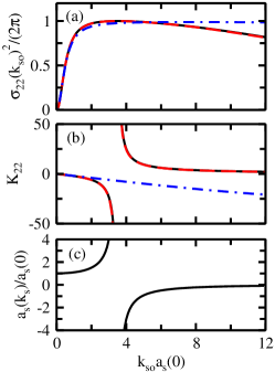
Figure 1: (Color online) Large $a_{s}(0)$ case. The black solid line shows (a) the scaled partial cross section $\sigma_{22}(k_{\text{so}})^{2}/(2\pi)$ and (b) the K-matrix element $K_{22}$ for $E=0$ as a function of $k_{\text{so}}a_{s}(0)$ for the Lennard-Jones potential with $a_{s}(0)/r_{\text{vdW}}=24.42$ and $V_{p}(0)/(r_{\text{vdW}})^{3}=-0.2380$ (this potential supports two $s$-wave bound states in free space). The red dashed line shows the result for the zero-range model developed in this work [see Eq. (15)]; the numerical results for the Lennard-Jones potential and the model are indistinguishable on the scale shown. To illustrate the importance of the energy shifts, the blue dash-dotted line shows the results for the zero-range model that artificially neglects the energy shifts. The solid line in (c) shows the scaled energy-dependent $s$-wave scattering length $a_{s}(k_{s})/a_{s}(0)$, where $\hbar^{2}k_{s}^{2}=6\mu E_{\text{so}}$.

To validate our analytical results, we perform numerical coupled-channels calculations. Since the wave function in the $J=0$ subspace is anti-symmetric under the simultaneous exchange of the spatial and spin degrees of freedom of the two particles, the solutions apply to two identical fermions. The Schrödinger equation for the Lennard-Jones potential $V_{\text{LJ}}(r)=C_{12}/r^{12}-C_{6}/r^{6}$, with $C_{6}$ and $C_{12}$ denoting positive coefficients, is solved numerically JCP_paper . The solid lines in Figs. 1 and 2 show the partial cross section $\sigma_{22}$ and the K-matrix element $K_{22}$ as a function of $k_{\text{so}}$ for vanishing scattering energy $E$ for a two-body potential with large $a_{s}(0)$ and large $V_{p}(0)$, respectively. The dashed lines show the results predicted by our zero-range model that accounts for the spin-orbit coupling induced energy shifts. This model provides an excellent description of the numerical results for the Lennard-Jones potential, provided the length $(k_{\text{so}})^{-1}$ associated with the spin-orbit coupling term is not too small compared to the van der Waals length $r_{\text{vdW}}$, where $r_{\text{vdW}}$ is given by $(2\mu C_{6}/\hbar^{2})^{1/4}$ (in Figs. 1 and 2, the largest $k_{\text{so}}r_{\text{vdW}}$ considered corresponds to $0.4913$ and $0.4171$, respectively).

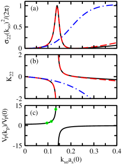
Figure 2: (Color online) Large $V_{p}(0)$ case. The black solid line shows (a) the scaled partial cross section $\sigma_{22}(k_{\text{so}})^{2}/(2\pi)$ and (b) the K-matrix element $K_{22}$ for $E=0$ as a function of $k_{\text{so}}a_{s}(0)$ for the Lennard-Jones potential with $a_{s}(0)/r_{\text{vdW}}=0.9591$ and $V_{p}(0)/(r_{\text{vdW}})^{3}=26.61$, corresponding to $a_{s}(0)/(V_{p}(0))^{1/3}=0.3213$ (this potential supports 4 four $s$-wave bound states in free space). The red dashed line shows the result for the zero-range model developed in this work [see Eq. (15)]; the model reproduces the numerical results excellently for $k_{\text{so}}a_{s}(0)\lesssim 0.3$. The blue dash-dotted line shows the results for the zero-range model that artificially neglects the energy shifts. The solid line in (c) shows the scaled energy-dependent $p$-wave scattering volume $V_{p}(k_{p})/V_{p}(0)$, where $\hbar^{2}k_{p}^{2}=-2\mu E_{\text{so}}$. The green circles mark three of the four $k_{\text{so}}a_{s}(0)$ values considered in Fig. 4.

The dash-dotted lines in Figs. 1 and 2 show $\sigma_{22}$ and $K_{22}$ for the zero-range model when we set the spin-orbit coupling induced energy shifts artificially to zero. In this case, the divergence in the $K_{22}$ matrix element at finite $k_{\text{so}}$ is not reproduced. For large $a_{s}(0)$ [see Fig. 1(a)], the model without energy shifts introduces deviations at the few percent level in the cross section $\sigma_{22}$. For large $V_{p}(0)$ [see Fig. 2(a)], in contrast, the model without the energy shifts provides a quantitatively and qualitatively poor description of the cross section $\sigma_{22}$ even for relatively small $k_{\text{so}}$ ($k_{\text{so}}a_{s}(0)\gtrsim 0.05$). Figures 1(c) and 2(c) demonstrate that the divergence of the $K_{22}$ matrix element occurs when the free-space scattering length $a_{s}(k_{s})$, calculated at energy $3E_{\text{so}}$, or the free-space scattering volume $V_{p}(k_{p})$, calculated at energy $-E_{\text{so}}$, diverge. We find that this occurs roughly when $a_{s}(0)k_{\text{so}}\approx 10$ and $(V_{p}(0))^{1/3}k_{\text{so}}\approx 0.21$; we checked that this holds quite generally, i.e., not only for the parameters considered in the figures. In Figs. 1(c) and 2(c), the “critical” $k_{\text{so}}$ values correspond to $k_{\text{so}}r_{\text{vdW}}=0.1423$ and $k_{\text{so}}r_{\text{vdW}}=0.1462$, respectively. For comparison, using the $k_{\text{so}}$ value for the one-dimensional realization of Ref. spielman and assuming $r_{\text{vdW}}=100a_{0}$, one finds $k_{\text{so}}r_{\text{vdW}}\approx 0.03$. This suggests that the phenomena discussed in the context of Figs. 1 and 2 should be relevant to future realizations of three-dimensional isotropic spin-orbit coupling experiments.

To further explore the two-particle scattering properties in the presence of spin-orbit coupling for short-range potentials with large free-space scattering volume $V_{p}(0)$, Figs. 3(a) and 3(b) show the partial cross section $\sigma_{22}$ as a function of the scattering energy $-E_{\text{so}}\leq E\leq 0$ and $0\leq 0\leq 400E_{\text{so}}$, respectively, for $a_{s}(0)/(V_{p}(0))^{1/3}=0.3213$ and $a_{s}(0)k_{\text{so}}=0.07673$. The results for the Lennard-Jones potential (dashed line) and square-well potential (solid line) are essentially indistinguishable on the scale shown. To assess the accuracy of our zero-range model, we focus on the Lennard-Jones potential and compare the numerically determined partial cross section $(\sigma_{22})^{\text{exact}}$ with the partial cross section $(\sigma_{22})^{\text{zr}}$ predicted using Eq. (15). Solid lines in Figs. 3(c) and 3(d) show the normalized difference $\Delta$, defined through $\Delta=|(\sigma_{22})^{\text{zr}}-(\sigma_{22})^{\text{exact}}|/(\sigma_{22})^{\text{exact}}$. The deviations are smaller than $1.3$% for the scattering energies considered. Neglecting the spin-orbit coupling induced energy shifts in our zero-range model and calculating the normalized difference, we obtain the dashed lines in Figs. 3(c) and 3(d). Clearly, the zero-range model provides a faithful description of the full coupled-channels data for the Lennard-Jones potential only if the spin-orbit coupling induced energy shifts are included.

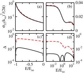
Figure 3: (Color online) Large $V_{p}(0)$ case. (a) and (b): The red dashed and black solid lines show the scaled partial cross section $\sigma_{22}(k_{\text{so}})^{2}/(2\pi)$ for the Lennard-Jones and square-well potential, respectively, as a function of the scattering energy $E$. For both potentials, we have $a_{s}(0)/(V_{p}(0))^{1/3}=0.3213$ [$V_{p}(0)>0$] and $k_{\text{so}}a_{s}(0)=0.07673$. The length scale associated with the spin-orbit coupling is notably larger than the range of the potential ($k_{\text{so}}r_{\text{vdW}}=0.08$ for the Lennard-Jones potential and $k_{\text{so}}r_{\text{sw}}=0.07676$ for the square-well potential). (c) and (d): The solid and dashed lines show the normalized difference $\Delta$ (see text) between the cross section for the Lennard-Jones potential and the zero-range model, obtained using Eq. (15), and between that for the Lennard-Jones potential and the zero-range model that neglects the spin-orbit coupling induced energy shifts, respectively. The zero-range model derived in this work (solid line) provides an excellent description (the deviations are smaller than $1.3$ % for the data shown) over the entire energy regime. Panels (a) and (c) cover negative $E$ (linear scale) while panels (b) and (d) cover positive $E$ (logarithmic scale)].

Figure 4 demonstrates that the non-quadratic single-particle dispersion relations have a profound impact on the low-energy scattering observables for a large free-space scattering volume. Specifically, the lines in Fig. 4 show the numerically obtained partial cross section $\sigma_{22}$ as a function of the scattering energy for the same Lennard-Jones potential as that used in Figs. 2 and 3 for four different spin-orbit coupling strengths, namely $k_{\text{so}}r_{\text{vdW}}=0.1$, $0.12$, $0.14$ and $0.146$ [Fig. 3 used $k_{\text{so}}r_{\text{vdW}}=0.08$; three of the four $k_{\text{so}}$ values considered in Fig. 4 are marked by circles in Fig. 2(c)]. Figure 4 shows that the partial cross section depends sensitively on the spin-orbit coupling strength $k_{\text{so}}$. This can be understood by realizing that a change in the spin-orbit coupling strength leads to a significant change of the $k_{\text{so}}$-dependent scattering volume $V_{p}(k_{p})$.

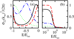
Figure 4: (Color online) Scaled partial cross section $\sigma_{22}(k_{\text{so}})^{2}/(2\pi)$ for the Lennard-Jones potential with $a_{s}(0)/(V_{p}(0))^{1/3}=0.3213$ ($V_{p}(0)>0$) and $a_{s}(0)/r_{\text{vdW}}=0.9591$ for four different $k_{\text{so}}$ [the green dotted, blue dash-dotted, black solid, and red dashed lines correspond to $k_{\text{so}}r_{\text{vdW}}=0.1$, $k_{\text{so}}r_{\text{vdW}}=0.12$, $k_{\text{so}}r_{\text{vdW}}=0.14$, and $k_{\text{so}}r_{\text{vdW}}=0.146$, respectively] as a function of the scattering energy $E$ [panel (a) covers negative $E$ (linear scale) while panel (b) covers positive $E$ (logarithmic scale)].

This paper revisited two-body scattering in the presence of single-particle interaction terms that lead, in the absence of two-body interactions, to non-quadratic dispersion relations. Restricting ourselves to three-dimensional isotropic spin-orbit coupling terms and spin-independent central two-body interactions, we developed an analytical coupled-channels theory that connects the short- and large-distance eigenfunctions using a generalized frame transformation. A key, previously overlooked result of our treatment is that the gauge transformation that converts the short-distance Hamiltonian to the “usual form” (i.e., a form without linear momentum dependence) introduces channel-dependent energy shifts. These energy shifts were then shown to appreciably alter the low-energy scattering observables, especially in the regime where the free-space scattering volume is large. To illustrate this, the $(J,M_{J})=(0,0)$ channel was considered exemplarily. Our framework provides the first complete analytical description that consistently accounts for all partial wave channels. Moreover, the first numerical coupled-channels results for two-particle Hamiltonian with realistic Lennard-Jones potentials in the presence of spin-orbit coupling terms were presented. The influence of the revised zero-range formulation put forward in this paper on two- and few-body bound states and on mean-field and beyond mean-field studies will be the topic of future publications.

I acknowledgement

Support by the National Science Foundation through grant number PHY-1509892 is gratefully acknowledged. The authors acknowledge hospitality of and support (National Science Foundation under Grant No. NSF PHY-1125915) by the KITP. We thank J. Jacob for providing us with a copy of his coupled-channels code.

References

- (1) C. Chin, R. Grimm, P. Julienne, and E. Tiesinga, Feshbach resonances in ultracold gases, Rev. Mod. Phys. 82, 1225 (2010).
- (2) I. Bloch, J. Dalibard, and W. Zwerger, Many-body physics with ultracold gases, Rev. Mod. Phys. 80, 885 (2008).
- (3) Theory of ultracold atomic Fermi gases, S. Giorgini, L. P. Pitaevskii, and S. Stringari, Rev. Mod. Phys. 80, 1215 (2008).
- (4) Y.-J. Lin, K. Jiménez-García, and I. B. Spielman, Spin-orbit-coupled Bose-Einstein condensates, Nature (London) 471, 83 (2011).
- (5) J. Dalibard, F. Gerbier, G. Juzeliūnas, and P. Öhberg, Colloquium: Artificial gauge potentials for neutral atoms, Rev. Mod. Phys. 83, 1523 (2011).
- (6) V. Galitski and I. B. Spielman, Spin-orbit coupling in quantum gases, Nature 494, 49 (2013).
- (7) H. Zhai, Degenerate quantum gases with spin-orbit coupling: a review, Rep. Prog. Phys. 78, 026001 (2015).
- (8) H. Zhai, Spin-Orbit Coupled Quantum Gases, Int. J. Mod. Phys. B 26, 1230001 (2012).
- (9) X. Cui, Mixed-partial-wave scattering with spin-orbit coupling and validity of pseudopotentials, Phys. Rev. A 85, 022705 (2012).
- (10) P. Zhang, L. Zhang, and Y. Deng, Modified Bethe-Peierls boundary condition for ultracold atoms with spin-orbit coupling, Phys. Rev. A 86, 053608 (2012).
- (11) Z. Yu, Short-range correlations in dilute atomic Fermi gases with spin-orbit coupling, Phys. Rev. A 85, 042711 (2012).
- (12) L. Zhang, Y. Deng, and P. Zhang, Scattering and effective interactions of ultracold atoms with spin-orbit coupling, Phys. Rev. A 87, 053626 (2013).
- (13) H. Duan, L. You, and B. Gao, Ultracold collisions in the presence of synthetic spin-orbit coupling, Phys. Rev. A 87, 052708 (2013).
- (14) Y. -C. Zhang, S. -W. Song, W. -M. Liu, The confinement induced resonance in spin-orbit coupled cold atoms with Raman coupling, Sci. Rep. 4, 4992 (2014).
- (15) S.-J. Wang and C. H. Greene, General formalism for ultracold scattering with isotropic spin-orbit coupling, Phys. Rev. A 91, 022706 (2015).
- (16) Q. Guan and D. Blume, Scattering framework for two particles with isotropic spin-orbit coupling applicable to all energies, Phys. Rev. A 94, 022706 (2016).
- (17) Y. Wu and Z. Yu, Short-range asymptotic behavior of the wave functions of interacting spin-1/2 fermionic atoms with spin-orbit coupling: A model study, Phys. Rev. A 87, 032703 (2013).
- (18) D. Blume and C. H. Greene, Fermi pseudopotential approximation: Two particles under external confinement, Phys. Rev. A 65, 043613 (2002).
- (19) E. L. Bolda, E. Tiesinga, and P. S. Julienne, Effective-scattering-length model of ultracold atomic collisions and Feshbach resonances in tight harmonic traps, Phys. Rev. A 66, 013403 (2002).
- (20) Here and in what follows, underlined quantities are matrices.
- (21) U. Fano, Stark effect of nonhydrogenic Rydberg spectra, Phys. Rev. A 24, 619(R), (1981).
- (22) D. A. Harmin, Theory of the Nonhydrogenic Stark Effect, Phys. Rev. Lett. 49, 128 (1982).
- (23) C. H. Greene, Negative-ion photodetachment in a weak magnetic field, Phys. Rev. A 36, 4236 (1987).
- (24) B. E. Granger and D. Blume, Tuning the Interactions of Spin-Polarized Fermions Using Quasi-One-Dimensional Confinement, Phys. Rev. Lett. 92, 133202 (2004).
- (25) S.-J. Wang, Ph.D thesis, Purdue University (2016).
- (26) B. R. Johnson, The Multichannel Log-Derivative Method for Scattering Calculations, J. Comput. Phys. 13, 445 (1973).
- (27) F. Mrugała and D. Secrest, The generalized log-derivative method for inelastic and reactive collisions, J. Chem. Phys. 78, 5954 (1983).