An Arrow-Hurwicz-Uzawa Type Flow as Least Squares Solver for Network Linear Equations

Yang Liu, Christian Lageman, Brian D. O. Anderson, and Guodong Shi Y. Liu, B. D. O. Anderson, and G. Shi are with the Research School of Engineering, The Australian National University, ACT 0200, Canberra, Australia. C. Lageman is with Institute of Mathematics, University of Würzburg, Würzburg 97070, Germany. Email: yang.liu@anu.edu.au, christian.lageman@mathematik.uni-wuerzburg.de, brian.anderson@anu.edu.au, guodong.shi@anu.edu.au
Abstract

We study the approach to obtaining least squares solutions to systems of linear algebraic equations over networks by using distributed algorithms. Each node has access to one of the linear equations and holds a dynamic state. The aim for the node states is to reach a consensus as a least squares solution of the linear equations by exchanging their states with neighbors over an underlying interaction graph. A continuous-time distributed least squares solver over networks is developed in the form of the famous Arrow-Hurwicz-Uzawa flow. A necessary and sufficient condition is established on the graph Laplacian for the continuous-time distributed algorithm to give the least squares solution in the limit, with an exponentially fast convergence rate. The feasibility of different fundamental graphs is discussed including path graph, star graph, etc. Moreover, a discrete-time distributed algorithm is developed by Euler’s method, converging exponentially to the least squares solution at the node states with suitable step size and graph conditions. The exponential convergence rate for both the continuous-time and discrete-time algorithms under the established conditions is confirmed by numerical examples. Finally, we investigate the performance of the proposed flow under switching networks, and surprisingly, switching networks at high switching frequencies can lead to approximate least square solvers even if all graphs in the switching signal fail to do so in the absence of structure switching.

Keywords: Distributed Algorithms; Dynamical Systems; Linear Equations; Least Squares; Switching Networks.

1 Introduction

Linear algebraic equations are foundational for various computation tasks, and systems of linear algebraic equations also arise from various practical engineering problems [11, 17, 30, 32, 9, 5, 8]. In recent years much interest has developed in finding out how to solve linear equations using multiple processing units or over a network. Major efforts have been made in the development of parallel or distributed algorithms as linear-equation solvers. On the one hand one aims at faster algorithms in view of the intuition that multiple processing units working in parallel under smart arrangements might provide significant improvements in computation efficiency. On the other hand various distributed systems induce structure constraints, e.g., one node holds one equation and it cannot or does not want to share the exact equation with other nodes, a constraint which excludes the feasibility of classical centralized algorithms.

Parallel algorithms for linear equations have been developed in the spirit of high-performance computing, e.g., the Jacobi method [23, 37], the successive over-relaxations method [38], the Kaczmarz method [16] and the randomized iterative method [14]. In these algorithms, the state of each node can give an entry of the solution to a linear equation after a suitably long running time, via successive information exchange with other nodes and parallel independent computing. There are two restrictions in these parallel algorithms. The first restriction is that often each node is implicitly required to have access to all the other ones, i.e., the network graph is naturally complete [23, 37, 16, 14]. Second, linear equations are restricted in many parallel algorithms. It is somewhat unsatisfactory that, for example in the Jacobi method, a sufficient condition for convergence is that the linear equations must be strictly or irreducibly diagonally dominant.

Meanwhile, discrete and continuous-time algorithms for linear equations known to have a unique solution are also established from the point of view of distributed control and optimization. A variety of distributed algorithms are presented, among which discrete-time algorithms are given by [25, 26, 20, 21, 22] and continuous-time algorithms are presented in [3, 33]. In these network distributed algorithms, compared with the development in parallel computing, each node state asymptotically converges to the solution to the linear equation. Such developments on network linear equations are closely related to, and sometimes even special cases of, the study of distributed optimization methods on nonlinear models [34, 27, 28, 13, 15], due to the natural connection between solving equations and optimizing objective functions.

Most of the existing work for parallel and distributed algorithms assumes that the linear equations have exact solutions [23, 37, 38, 16, 14, 25, 26, 20, 21, 22, 3], or can only produce least square solutions in the approximate sense or for limited graph structures [33], and very few results have been obtained on exact distributed least squares solvers for network linear equations. In this paper, distributed continuous and discrete-time algorithms that can compute the least squares solution to a linear equation over a network are presented. The particular contributions of our work are summarized as follows.

  • By recognizing a least-squares problem for a linear equation as a constrained optimization problem over a network, a continuous-time flow is presented in the form of the classical Arrow-Hurwicz-Uzawa flow [4], for which we establish necessary and sufficient conditions regarding which graph structures can drive the network flow to agree on the least squares solution.

  • By Euler’s method, a discrete-time algorithm is presented and the properties of its convergence are also specified and proved.

  • Comprehensive discussions on the residual vector, an alternative state expansion method, and switching networks are provided. Surprisingly, it can be shown that under a sufficiently fast switching signal, the proposed flow for switching networks becomes an approximate least square solver under which node states are driven to at least a small neighborhood around the least square solution, even if all graphs in the switching signal fail to do so in the absence of structure switching.

The paper begins by the formulating the network linear equations in Section 2, in addition to explaining how the Arrow-Hurwicz-Uzawa flow can be used to derive a continuous-time network flow. In Section 3, a necessary and sufficient condition for the continuous-time flow to converge to the least squares solution is established, along with its proof and a couple of numerical examples. In Section 4, a discrete-time algorithm is obtained by Euler’s method and the necessary and sufficient conditions for its convergence conditions are established, and a few numerical examples are also given. In Section 5, we further discuss distributed computation of residual vector, alternative methods of obtaining the least squares solution, and a few numerical examples to study the convergence properties of the continuous-time algorithm over a switching network. Finally a few concluding remarks are given in Section 6.

2 Problem Definition

2.1 Linear Equation

Consider the following linear algebraic equation with unknown 𝐲m𝐲superscript𝑚\mathbf{y}\in\mathbb{R}^{m}:

𝐳=𝐇𝐲𝐳𝐇𝐲\mathbf{z}=\mathbf{H}\mathbf{y} (1)

and where 𝐳N𝐳superscript𝑁\mathbf{z}\in\mathbb{R}^{N} and 𝐇N×m𝐇superscript𝑁𝑚\mathbf{H}\in\mathbb{R}^{N\times m} are known. Denote the column space of a matrix 𝐌𝐌\mathbf{M} by colsp{𝐌}colsp𝐌\operatorname{colsp}\{\mathbf{M}\}. If 𝐳colsp{𝐇}𝐳colsp𝐇\mathbf{z}\in\operatorname{colsp}\{\mathbf{H}\}, then the equation (1) always has (one or many) exact solutions. If 𝐳colsp{𝐇}𝐳colsp𝐇\mathbf{z}\notin\operatorname{colsp}\{\mathbf{H}\}, the least squares solution is defined by the solution of the following optimization problem:

min𝐲m𝐳𝐇𝐲2.subscript𝐲superscript𝑚superscriptnorm𝐳𝐇𝐲2\min_{\mathbf{y}\in\mathbb{R}^{m}}\|\mathbf{z}-\mathbf{H}\mathbf{y}\|^{2}. (2)

It is well known that if rank(𝐇)=mrank𝐇𝑚\operatorname{rank}(\mathbf{H})=m, then (2) yields a unique solution 𝐲=(𝐇𝐇)1𝐇𝐳superscript𝐲superscriptsuperscript𝐇top𝐇1superscript𝐇top𝐳\mathbf{y}^{\ast}=(\mathbf{H}^{\top}\mathbf{H})^{-1}\mathbf{H}^{\top}\mathbf{z}.

2.2 Network

Denote

H=[𝐡1𝐡2𝐡N],𝐳=[z1z2zN].formulae-sequence𝐻matrixsuperscriptsubscript𝐡1topsuperscriptsubscript𝐡2topsuperscriptsubscript𝐡𝑁top𝐳matrixsubscript𝑧1subscript𝑧2subscript𝑧𝑁H=\begin{bmatrix}\mathbf{h}_{1}^{\top}\\ \mathbf{h}_{2}^{\top}\\ \vdots\\ \mathbf{h}_{N}^{\top}\end{bmatrix},\quad\mathbf{z}=\begin{bmatrix}z_{1}\\ z_{2}\\ \vdots\\ z_{N}\end{bmatrix}.

We can rewrite (1) as

𝐡i𝐲=zi,i=1,,N.formulae-sequencesuperscriptsubscript𝐡𝑖top𝐲subscript𝑧𝑖𝑖1𝑁\mathbf{h}_{i}^{\top}\mathbf{y}=z_{i},\ i=1,\dots,N.

Let 𝒢=(𝒱,)𝒢𝒱\mathcal{G}=(\mathcal{V},\mathcal{E}) be a constant, undirected and connected graph with the set of nodes 𝒱={1,2,,N}𝒱12𝑁\mathcal{V}=\{1,2,\dots,N\} and the set of edges 𝒱×𝒱𝒱𝒱\mathcal{E}\subset\mathcal{V}\times\mathcal{V}. Each node i𝑖i holds the equation 𝐡i𝐲=zisuperscriptsubscript𝐡𝑖top𝐲subscript𝑧𝑖\mathbf{h}_{i}^{\top}\mathbf{y}=z_{i} and also holds a vector 𝐱i(t)msubscript𝐱𝑖𝑡superscript𝑚\mathbf{x}_{i}(t)\in\mathbb{R}^{m} that varies as a function of time t𝑡t. Note that 𝐱i(t)subscript𝐱𝑖𝑡\mathbf{x}_{i}(t) will turn out to be part of the state of node i𝑖i at time t𝑡t. Let 𝒩isubscript𝒩𝑖\mathcal{N}_{i} be the set of neighbor nodes that are connected to node i𝑖i, i.e., 𝒩i={j:(i,j)}subscript𝒩𝑖conditional-set𝑗𝑖𝑗\mathcal{N}_{i}=\{j:(i,j)\in\mathcal{E}\}. Define a diagonal matrix 𝐃=diag(|𝒩1|,|𝒩2|,,|𝒩N|)𝐃diagsubscript𝒩1subscript𝒩2subscript𝒩𝑁\mathbf{D}=\operatorname{diag}(|\mathcal{N}_{1}|,|\mathcal{N}_{2}|,\dots,|\mathcal{N}_{N}|) and an incidence matrix 𝐀𝐀\mathbf{A} of the graph 𝒢𝒢\mathcal{G} by [𝐀]ij=1subscriptdelimited-[]𝐀𝑖𝑗1[\mathbf{A}]_{ij}=1 if (i,j)𝑖𝑗(i,j)\in\mathcal{E} and [𝐀]ij=0subscriptdelimited-[]𝐀𝑖𝑗0[\mathbf{A}]_{ij}=0 otherwise. Then 𝐋=𝐃𝐀𝐋𝐃𝐀\mathbf{L}=\mathbf{D}-\mathbf{A} is the Laplacian of graph 𝒢𝒢\mathcal{G}.

2.3 Distributed Flows

Consider a cost function U():m××m:𝑈superscript𝑚superscript𝑚U(\cdot):\mathbb{R}^{m}\times\dots\times\mathbb{R}^{m}\to\mathbb{R}

U(𝐱1,,𝐱N)=i=1N|𝐡i𝐱izi|2.𝑈subscript𝐱1subscript𝐱𝑁superscriptsubscript𝑖1𝑁superscriptsuperscriptsubscript𝐡𝑖topsubscript𝐱𝑖subscript𝑧𝑖2U(\mathbf{x}_{1},\dots,\mathbf{x}_{N})=\sum_{i=1}^{N}|\mathbf{h}_{i}^{\top}\mathbf{x}_{i}-z_{i}|^{2}. (3)

Let 𝐱(t)=[𝐱1(t)𝐱N(t)]𝐱𝑡superscriptdelimited-[]superscriptsubscript𝐱1top𝑡superscriptsubscript𝐱𝑁top𝑡top\mathbf{x}(t)=[\mathbf{x}_{1}^{\top}(t)\ \dots\ \mathbf{x}_{N}^{\top}(t)]^{\top} and introduce 𝐯(t)=[𝐯1(t)𝐯N(t)]𝐯𝑡superscriptdelimited-[]superscriptsubscript𝐯1top𝑡superscriptsubscript𝐯𝑁top𝑡top\mathbf{v}(t)=[\mathbf{v}_{1}^{\top}(t)\ \dots\ \mathbf{v}_{N}^{\top}(t)]^{\top} with 𝐯i(t)msubscript𝐯𝑖𝑡superscript𝑚\mathbf{v}_{i}(t)\in\mathbb{R}^{m} for i=1,,N𝑖1𝑁i=1,\dots,N. The vector 𝐯i(t)subscript𝐯𝑖𝑡\mathbf{v}_{i}(t) is also held by node i𝑖i, and the 2m2𝑚2m-dimensional vector [𝐱i(t)𝐯i(t)]superscriptdelimited-[]subscript𝐱𝑖superscript𝑡topsubscript𝐯𝑖superscript𝑡toptop[\mathbf{x}_{i}(t)^{\top}\ \mathbf{v}_{i}(t)^{\top}]^{\top} represents the state of node i𝑖i.

We consider the following flow:

𝐱˙˙𝐱\displaystyle\dot{\mathbf{x}} =(𝐋𝐈m)𝐯U(𝐱)absenttensor-product𝐋subscript𝐈𝑚𝐯𝑈𝐱\displaystyle=-(\mathbf{L}\otimes\mathbf{I}_{m})\mathbf{v}-\nabla U(\mathbf{x}) (4)
𝐯˙˙𝐯\displaystyle\dot{\mathbf{v}} =(𝐋𝐈m)𝐱.absenttensor-product𝐋subscript𝐈𝑚𝐱\displaystyle=(\mathbf{L}\otimes\mathbf{I}_{m})\mathbf{x}.

We term (4) an “Oscillation + Gradient Flow” because the equation

𝐱˙˙𝐱\displaystyle\dot{\mathbf{x}} =(𝐋𝐈m)𝐯absenttensor-product𝐋subscript𝐈𝑚𝐯\displaystyle=-(\mathbf{L}\otimes\mathbf{I}_{m})\mathbf{v}
𝐯˙˙𝐯\displaystyle\dot{\mathbf{v}} =(𝐋𝐈m)𝐱absenttensor-product𝐋subscript𝐈𝑚𝐱\displaystyle=(\mathbf{L}\otimes\mathbf{I}_{m})\mathbf{x}

yields oscillating trajectories for 𝐱(t)𝐱𝑡\mathbf{x}(t), while 𝐱˙=U(𝐱)˙𝐱𝑈𝐱\dot{\mathbf{x}}=-\nabla U(\mathbf{x}) is a gradient flow.

Note that in the flow (4), the state variable [𝐱i(t)𝐯i(t)]superscriptdelimited-[]subscriptsuperscript𝐱top𝑖𝑡subscriptsuperscript𝐯top𝑖𝑡top[\mathbf{x}^{\top}_{i}(t)\ \mathbf{v}^{\top}_{i}(t)]^{\top} of node i𝑖i obeys the evolution

𝐱˙i(t)subscript˙𝐱𝑖𝑡\displaystyle\dot{\mathbf{x}}_{i}(t) =j𝒩i(𝐯i(t)𝐯j(t))(𝐡i𝐡i𝐱i(t)zi𝐡i)absentsubscript𝑗subscript𝒩𝑖subscript𝐯𝑖𝑡subscript𝐯𝑗𝑡subscript𝐡𝑖superscriptsubscript𝐡𝑖topsubscript𝐱𝑖𝑡subscript𝑧𝑖subscript𝐡𝑖\displaystyle=-\sum_{j\in\mathcal{N}_{i}}(\mathbf{v}_{i}(t)-\mathbf{v}_{j}(t))-(\mathbf{h}_{i}\mathbf{h}_{i}^{\top}\mathbf{x}_{i}(t)-z_{i}\mathbf{h}_{i})
𝐯˙i(t)subscript˙𝐯𝑖𝑡\displaystyle\dot{\mathbf{v}}_{i}(t) =j𝒩i(𝐱i(t)𝐱j(t))absentsubscript𝑗subscript𝒩𝑖subscript𝐱𝑖𝑡subscript𝐱𝑗𝑡\displaystyle=\sum_{j\in\mathcal{N}_{i}}(\mathbf{x}_{i}(t)-\mathbf{x}_{j}(t))

Therefore, besides the equation 𝐡i𝐲=zisuperscriptsubscript𝐡𝑖top𝐲subscript𝑧𝑖\mathbf{h}_{i}^{\top}\mathbf{y}=z_{i} that node i𝑖i possesses, it only needs to communicate with its neighbors to obtain their states in order to implement (4). The flow (4) is distributed in that sense.

2.4 Discussions

2.4.1 Relation to A-H-U Flow

Consider a constrained optimization problem as

min𝐱subscript𝐱\displaystyle\min_{\mathbf{x}} f(𝐱)𝑓𝐱\displaystyle f(\mathbf{x}) (5)
s.t.formulae-sequencest\displaystyle{\rm s.t.} 𝐅𝐱=𝐛𝐅𝐱𝐛\displaystyle\mathbf{F}\mathbf{x}=\mathbf{b}

where f():n:𝑓superscript𝑛f(\cdot):\mathbb{R}^{n}\to\mathbb{R} is a differentiable function, 𝐅m×n𝐅superscript𝑚𝑛\mathbf{F}\in\mathbb{R}^{m\times n} and 𝐛m𝐛superscript𝑚\mathbf{b}\in\mathbb{R}^{m}. The well-known Arrow-Hurwicz-Uzawa (A-H-U) flow introduced in [4] provides under appropriate conditions a continuous-time solver defined by

𝐱˙˙𝐱\displaystyle\dot{\mathbf{x}} =𝐱f(𝐱)𝐅𝐯absentsubscript𝐱𝑓𝐱superscript𝐅top𝐯\displaystyle=-\nabla_{\mathbf{x}}f(\mathbf{x})-\mathbf{F}^{\top}\mathbf{v} (6)
𝐯˙˙𝐯\displaystyle\dot{\mathbf{v}} =𝐅𝐱𝐛.absent𝐅𝐱𝐛\displaystyle=\mathbf{F}\mathbf{x}-\mathbf{b}.

In particular, if f𝑓f is strictly convex and 𝐅𝐅\mathbf{F} has full row rank, then (see [4][36]) along the flow (6), 𝐱(t)𝐱𝑡\mathbf{x}(t) will converge to the optimal point of (5) and 𝐯(t)𝐯𝑡\mathbf{v}(t) will converge to a Lagrangian multiplier of (5).

As one can see, the flow (4) is a form of the A-H-U flow (6) with the cost function f(𝐱)𝑓𝐱f(\mathbf{x}) being the given U(𝐱)𝑈𝐱U(\mathbf{x}) and the constraint 𝐅𝐱=𝐛𝐅𝐱𝐛\mathbf{F}\mathbf{x}=\mathbf{b} given by (𝐋𝐈m)𝐱=0tensor-product𝐋subscript𝐈𝑚𝐱0(\mathbf{L}\otimes\mathbf{I}_{m})\mathbf{x}=0. However, neither the Laplacian 𝐋𝐋\mathbf{L} is a full-rank matrix, nor is U(𝐱)𝑈𝐱U(\mathbf{x}) strictly convex. Therefore, the sufficiency results and analysis for the A-H-U flow established in [36] cannot be applied directly to the flow (4).

2.4.2 Relation to Wang-Elia/Gharesifard-Cortés Flows

In [35] and [12], an alternative distributed flow for solving

min𝐱=(𝐱1𝐱N)subscript𝐱superscriptsuperscriptsubscript𝐱1topsuperscriptsubscript𝐱𝑁toptop\displaystyle\min_{\mathbf{x}=(\mathbf{x}_{1}^{\top}\dots\mathbf{x}_{N}^{\top})^{\top}} i=1Nfi(𝐱i)superscriptsubscript𝑖1𝑁subscript𝑓𝑖subscript𝐱𝑖\displaystyle\sum_{i=1}^{N}f_{i}(\mathbf{x}_{i}) (7)
s.t.formulae-sequencest\displaystyle{\rm s.t.} 𝐱im,i=1,,Nformulae-sequencesubscript𝐱𝑖superscript𝑚𝑖1𝑁\displaystyle\mathbf{x}_{i}\in\mathbb{R}^{m},i=1,\dots,N
𝐱1==𝐱Nsubscript𝐱1subscript𝐱𝑁\displaystyle\mathbf{x}_{1}=\dots=\mathbf{x}_{N}

was proposed, where each fi:m:subscript𝑓𝑖maps-tosuperscript𝑚f_{i}:\mathbb{R}^{m}\mapsto\mathbb{R} is a locally Lipschitz and convex function known to node i𝑖i only. Viewing the component |𝐡i𝐱izi|2superscriptsuperscriptsubscript𝐡𝑖topsubscript𝐱𝑖subscript𝑧𝑖2|\mathbf{h}_{i}^{\top}\mathbf{x}_{i}-z_{i}|^{2} in U(𝐱1,,𝐱N)𝑈subscript𝐱1subscript𝐱𝑁U(\mathbf{x}_{1},\dots,\mathbf{x}_{N}) as the fisubscript𝑓𝑖f_{i} in (7), the Wang-Elia/Gharesifard-Cortés flow [35, 12] reads as

𝐱˙˙𝐱\displaystyle\dot{\mathbf{x}} =α(𝐋𝐈m)𝐱(𝐋𝐈m)𝐯𝐇~𝐱+𝐳Habsent𝛼tensor-product𝐋subscript𝐈𝑚𝐱tensor-product𝐋subscript𝐈𝑚𝐯~𝐇𝐱subscript𝐳𝐻\displaystyle=-{\alpha}(\mathbf{L}\otimes\mathbf{I}_{m}){\mathbf{x}}-(\mathbf{L}\otimes\mathbf{I}_{m}){\mathbf{v}}-\tilde{\mathbf{H}}\mathbf{x}{+}\mathbf{z}_{H} (8)
𝐯˙˙𝐯\displaystyle\dot{\mathbf{v}} =(𝐋𝐈m)𝐱.absenttensor-product𝐋subscript𝐈𝑚𝐱\displaystyle=(\mathbf{L}\otimes\mathbf{I}_{m})\mathbf{x}.

where α𝛼\alpha is a positive number, 𝐳H=[z1𝐡1zH𝐡N]subscript𝐳𝐻superscriptdelimited-[]subscript𝑧1superscriptsubscript𝐡1topsubscript𝑧𝐻superscriptsubscript𝐡𝑁toptop\mathbf{z}_{H}=[z_{1}\mathbf{h}_{1}^{\top}\ \dots\ z_{H}\mathbf{h}_{N}^{\top}]^{\top} and 𝐇~=diag(𝐡1𝐡1,,𝐡N𝐡N)~𝐇diagsubscript𝐡1superscriptsubscript𝐡1topsubscript𝐡𝑁superscriptsubscript𝐡𝑁top\tilde{\mathbf{H}}=\operatorname{diag}(\mathbf{h}_{1}\mathbf{h}_{1}^{\top},\dots,\mathbf{h}_{N}\mathbf{h}_{N}^{\top}) since by direct calculation we know U(𝐱)=𝐇~𝐱𝐳H𝑈𝐱~𝐇𝐱subscript𝐳𝐻\nabla U(\mathbf{x})=\tilde{\mathbf{H}}\mathbf{x}-\mathbf{z}_{H}. With fixed interaction graph and suitable choice of α𝛼\alpha, the flow (8) is a least squares solver for (1) even for balanced directed networks (Theorem 5.4, [12]). The system (4) under consideration in the current work certainly has a simpler structure compared to (8), which is desirable in large-scale applications. Moreover, it is also useful to establish a clear understanding of the convergence conditions of the system (4) under general conditions (which are currently missing in the literature),the more so considering the historical context.

3 Continuous Flow

In this section, we study the behavior of the flow (4) in terms of convergence to a least squares solution for the 𝐱i(t)subscript𝐱𝑖𝑡\mathbf{x}_{i}(t), and present necessary and sufficient conditions for convergence.

3.1 Convergence Result

We present the following result.

Theorem 1

Assume that N>m𝑁𝑚N>m and rank(𝐇)=mrank𝐇𝑚\operatorname{rank}(\mathbf{H})=m. Let 𝐲=(𝐇𝐇)1𝐇𝐳superscript𝐲superscriptsuperscript𝐇top𝐇1superscript𝐇top𝐳\mathbf{y}^{\ast}=(\mathbf{H}^{\top}\mathbf{H})^{-1}\mathbf{H}^{\top}\mathbf{z} be the unique least squares solution of (1). Define 𝒮𝐋subscript𝒮𝐋\mathcal{S}_{\mathbf{L}} as the set of all complex eigenvectors of 𝐋𝐋\mathbf{L} and for 𝛂𝒮𝐋𝛂subscript𝒮𝐋\bm{\alpha}\in\mathcal{S}_{\mathbf{L}} with 𝛂[i]𝛂delimited-[]𝑖\bm{\alpha}[i] denoting the i𝑖i-th entry,

𝜶:={i:𝜶[i]0,𝜶=[𝜶[1]𝜶[2]𝜶[N]]}.assignsubscript𝜶conditional-set𝑖formulae-sequence𝜶delimited-[]𝑖0𝜶superscriptdelimited-[]𝜶delimited-[]1𝜶delimited-[]2𝜶delimited-[]𝑁top\mathcal{I}_{\bm{\alpha}}:=\{i:\bm{\alpha}[i]\neq 0,\ \bm{\alpha}=\big{[}\bm{\alpha}[1]\ \bm{\alpha}[2]\ \dots\ \bm{\alpha}[N]\big{]}^{\top}\}.

Then:

  1. (i)

    If span{𝐡i:i𝜶}=mspan:subscript𝐡𝑖𝑖subscript𝜶superscript𝑚\operatorname{span}\{\mathbf{h}_{i}:i\in\mathcal{I}_{\bm{\alpha}}\}=\mathbb{R}^{m} for all 𝜶𝒮𝐋𝜶subscript𝒮𝐋\bm{\alpha}\in\mathcal{S}_{\mathbf{L}}, there holds

    limt𝐱i(t)=𝐲,i=1,,Nformulae-sequencesubscript𝑡subscript𝐱𝑖𝑡superscript𝐲𝑖1𝑁\lim_{t\to\infty}\mathbf{x}_{i}(t)=\mathbf{y}^{\ast},i=1,\dots,N

    along the flow (4). Further 𝐯(t)𝐯𝑡\mathbf{v}(t) along (4) converges to a Lagrange multiplier associated with a solution of the optimization problem

    min𝐱subscript𝐱\displaystyle\min_{\mathbf{x}} U(𝐱)𝑈𝐱\displaystyle U(\mathbf{x}) (9)
    s.t.formulae-sequencest\displaystyle{\rm s.t.} (𝐋𝐈m)𝐱=0tensor-product𝐋subscript𝐈𝑚𝐱0\displaystyle(\mathbf{L}\otimes\mathbf{I}_{m})\mathbf{x}=0
  2. (ii)

    If there exists 𝜶𝒮𝐋𝜶subscript𝒮𝐋\bm{\alpha}\in\mathcal{S}_{\mathbf{L}} such that dim(span{𝐡i:i𝜶})<mdimensionspan:subscript𝐡𝑖𝑖subscript𝜶𝑚\dim(\operatorname{span}\{\mathbf{h}_{i}:i\in\mathcal{I}_{\bm{\alpha}}\})<m, then there exist trajectories of 𝐱(t)𝐱𝑡\mathbf{x}(t) along (4) which do not converge.

Proof. Recall that U(𝐱)=𝐇~𝐱𝐳H𝑈𝐱~𝐇𝐱subscript𝐳𝐻\nabla U(\mathbf{x})=\tilde{\mathbf{H}}\mathbf{x}-\mathbf{z}_{H} where 𝐇~~𝐇\tilde{\mathbf{H}} is the nonnegative matrix diag(𝐡1𝐡1,,𝐡N𝐡N)diagsubscript𝐡1superscriptsubscript𝐡1topsubscript𝐡𝑁superscriptsubscript𝐡𝑁top\operatorname{diag}(\mathbf{h}_{1}\mathbf{h}_{1}^{\top},\dots,\mathbf{h}_{N}\mathbf{h}_{N}^{\top}) and 𝐳H=[z1𝐡1zH𝐡N]subscript𝐳𝐻superscriptdelimited-[]subscript𝑧1superscriptsubscript𝐡1topsubscript𝑧𝐻superscriptsubscript𝐡𝑁toptop\mathbf{z}_{H}=[z_{1}\mathbf{h}_{1}^{\top}\ \dots\ z_{H}\mathbf{h}_{N}^{\top}]^{\top}. We rewrite (4) as

𝐱˙˙𝐱\displaystyle\dot{\mathbf{x}} =(𝐋𝐈m)𝐯𝐇~𝐱+𝐳Habsenttensor-product𝐋subscript𝐈𝑚𝐯~𝐇𝐱subscript𝐳𝐻\displaystyle=-(\mathbf{L}\otimes\mathbf{I}_{m})\mathbf{v}-\tilde{\mathbf{H}}\mathbf{x}+\mathbf{z}_{H} (10)
𝐯˙˙𝐯\displaystyle\dot{\mathbf{v}} =(𝐋𝐈m)𝐱.absenttensor-product𝐋subscript𝐈𝑚𝐱\displaystyle=(\mathbf{L}\otimes\mathbf{I}_{m})\mathbf{x}.

Suppose there exists an equilibrium (𝐱,𝐯)superscript𝐱superscript𝐯(\mathbf{x}^{\ast},\mathbf{v}^{\ast}) of (10), i.e.

00\displaystyle 0 =(𝐋𝐈m)𝐯𝐇~𝐱+𝐳Habsenttensor-product𝐋subscript𝐈𝑚superscript𝐯~𝐇superscript𝐱subscript𝐳𝐻\displaystyle=-(\mathbf{L}\otimes\mathbf{I}_{m})\mathbf{v}^{\ast}-\tilde{\mathbf{H}}\mathbf{x}^{\ast}+\mathbf{z}_{H} (11)
00\displaystyle 0 =(𝐋𝐈m)𝐱.absenttensor-product𝐋subscript𝐈𝑚superscript𝐱\displaystyle=(\mathbf{L}\otimes\mathbf{I}_{m})\mathbf{x}^{\ast}.

It is worth noting that (11) specifies exactly the Karush-Kuhn-Tucker conditions on (𝐱,𝐯)superscript𝐱superscript𝐯(\mathbf{x}^{\ast},\mathbf{v}^{\ast}) for the optimization problem (9) [6]. Since U(x)𝑈𝑥U(x) is a convex function and the constraints in (9) are equality constraints, Slater’s condition holds [7]. Therefore the optimal points of the primal problem and dual problem are the same, i.e., 𝐱superscript𝐱\mathbf{x}^{\ast} is an optimal solution to (9) and any optimal solution of (9) must have the form

𝟏𝐲,tensor-product1superscript𝐲\mathbf{1}\otimes\mathbf{y}^{\ast},

where 𝐲superscript𝐲\mathbf{y}^{\ast} is a least squares solution to (1). We know 𝐲superscript𝐲\mathbf{y}^{\ast} is unique because rank(𝐇)=mrank𝐇𝑚\operatorname{rank}(\mathbf{H})=m. Since 𝐱=1𝐲superscript𝐱tensor-product1superscript𝐲\mathbf{x}^{\ast}=1\otimes\mathbf{y}^{\ast}, then 𝐱superscript𝐱\mathbf{x}^{\ast} is also unique. Note however that 𝐯superscript𝐯\mathbf{v}^{\ast} is not necessarily unique. Define the variables 𝐱^=𝐱𝐱^𝐱𝐱superscript𝐱\hat{\mathbf{x}}=\mathbf{x}-\mathbf{x}^{\ast}, 𝐯^=𝐯𝐯^𝐯𝐯superscript𝐯\hat{\mathbf{v}}=\mathbf{v}-\mathbf{v}^{\ast}. Then

𝐱^˙˙^𝐱\displaystyle\dot{\hat{\mathbf{x}}} =𝐱˙𝐱˙=(𝐋𝐈m)𝐯^𝐇~𝐱^absent˙𝐱superscript˙𝐱tensor-product𝐋subscript𝐈𝑚^𝐯~𝐇^𝐱\displaystyle=\dot{\mathbf{x}}-\dot{\mathbf{x}}^{\ast}=-(\mathbf{L}\otimes\mathbf{I}_{m})\hat{\mathbf{v}}-\tilde{\mathbf{H}}\hat{\mathbf{x}} (12)
𝐯^˙˙^𝐯\displaystyle\dot{\hat{\mathbf{v}}} =(𝐋𝐈m)𝐱^.absenttensor-product𝐋subscript𝐈𝑚^𝐱\displaystyle=(\mathbf{L}\otimes\mathbf{I}_{m})\hat{\mathbf{x}}.

Denote 𝐮^(t)=[𝐱^(t)𝐯^(t)]^𝐮𝑡superscriptdelimited-[]^𝐱superscript𝑡top^𝐯superscript𝑡toptop\hat{\mathbf{u}}(t)=[{\hat{\mathbf{x}}}(t)^{\top}\ {\hat{\mathbf{v}}}(t)^{\top}]^{\top} and

𝐌=[𝐇~𝐋𝐈m𝐋𝐈m0].𝐌matrix~𝐇tensor-product𝐋subscript𝐈𝑚tensor-product𝐋subscript𝐈𝑚0\mathbf{M}=\begin{bmatrix}-\tilde{\mathbf{H}}&-\mathbf{L}\otimes\mathbf{I}_{m}\\ \mathbf{L}\otimes\mathbf{I}_{m}&0\end{bmatrix}.

Then (12) is a linear system with the form 𝐮^˙=𝐌𝐮^˙^𝐮𝐌^𝐮\dot{\hat{\mathbf{u}}}=\mathbf{M}\hat{\mathbf{u}}. Consider the following Lyapunov function:

V(𝐱^,𝐯^)=12𝐮^2=12(𝐱^2+𝐯^2).𝑉^𝐱^𝐯12superscriptnorm^𝐮212superscriptnorm^𝐱2superscriptnorm^𝐯2V(\hat{\mathbf{x}},\hat{\mathbf{v}})=\frac{1}{2}\|\hat{\mathbf{u}}\|^{2}=\frac{1}{2}(\|\hat{\mathbf{x}}\|^{2}+\|\hat{\mathbf{v}}\|^{2}).

Since

V˙˙𝑉\displaystyle\dot{V} =𝐱^(𝐋𝐈m)𝐯^𝐱^𝐇~𝐱+𝐯^(𝐋𝐈m)𝐱^absentsuperscript^𝐱toptensor-product𝐋subscript𝐈𝑚^𝐯superscript^𝐱top~𝐇𝐱superscript^𝐯toptensor-product𝐋subscript𝐈𝑚^𝐱\displaystyle=-\hat{\mathbf{x}}^{\top}(\mathbf{L}\otimes\mathbf{I}_{m})\hat{\mathbf{v}}-\hat{\mathbf{x}}^{\top}\tilde{\mathbf{H}}\mathbf{x}+\hat{\mathbf{v}}^{\top}(\mathbf{L}\otimes\mathbf{I}_{m})\hat{\mathbf{x}} (13)
=𝐱^𝐇~𝐱^0,absentsuperscript^𝐱top~𝐇^𝐱0\displaystyle=-\hat{\mathbf{x}}^{\top}\tilde{\mathbf{H}}\hat{\mathbf{x}}\leq 0,

𝐮^(t)^𝐮𝑡\hat{\mathbf{u}}(t) is bounded for any finite initial values 𝐱^(0)^𝐱0\hat{\mathbf{x}}(0), 𝐯^(0)^𝐯0\hat{\mathbf{v}}(0), namely 𝐮^(0)^𝐮0\hat{\mathbf{u}}(0). Therefore, we conclude:

C1. (λ)0𝜆0\Re(\lambda)\leq 0 for all λσ(𝐌)𝜆𝜎𝐌\lambda\in\sigma(\mathbf{M}).

C2. If (λ)=0𝜆0\Re(\lambda)=0, then λ𝜆\lambda has equal algebraic and geometric multiplicity.

(i). Suppose span{𝐡i:i𝜶}=mspan:subscript𝐡𝑖𝑖subscript𝜶superscript𝑚\operatorname{span}\{\mathbf{h}_{i}:i\in\mathcal{I}_{\bm{\alpha}}\}=\mathbb{R}^{m} for all 𝜶𝒮𝐋𝜶subscript𝒮𝐋\bm{\alpha}\in\mathcal{S}_{\mathbf{L}}. We proceed to prove the convergence of 𝐱^(t)^𝐱𝑡\hat{\mathbf{x}}(t) and 𝐯^(t)^𝐯𝑡\hat{\mathbf{v}}(t). The proof contains two steps.

Step 1. We prove 𝐌𝐌\mathbf{M} does not have a purely imaginary eigenvalue if span{𝐡i:i𝜶}=mspan:subscript𝐡𝑖𝑖subscript𝜶superscript𝑚\operatorname{span}\{\mathbf{h}_{i}:i\in\mathcal{I}_{\bm{\alpha}}\}=\mathbb{R}^{m} for all 𝜶𝒮𝐋𝜶subscript𝒮𝐋\bm{\alpha}\in\mathcal{S}_{\mathbf{L}}, using a contradiction argument. Thus suppose λ=ır0𝜆italic-ı𝑟0\lambda=\imath r\neq 0 where r𝑟r\in\mathbb{R} is an eigenvalue of 𝐌𝐌\mathbf{M} with a corresponding eigenvector 𝜷=[𝜷a𝜷b]2Nm𝜷delimited-[]superscriptsubscript𝜷𝑎topsuperscriptsubscript𝜷𝑏topsuperscript2𝑁𝑚\bm{\beta}=[\bm{\beta}_{a}^{\top}\ \bm{\beta}_{b}^{\top}]\in\mathbb{C}^{2Nm}, where 𝜷aNmsubscript𝜷𝑎superscript𝑁𝑚\bm{\beta}_{a}\in\mathbb{C}^{Nm}, 𝜷bNmsubscript𝜷𝑏superscript𝑁𝑚\bm{\beta}_{b}\in\mathbb{C}^{Nm}. Let 𝐮^(0)=𝜷^𝐮0𝜷\hat{\mathbf{u}}(0)=\bm{\beta}. Then

𝐮^(t)=e𝐌t𝐮^(0)=eırt𝐮^(0).^𝐮𝑡superscript𝑒𝐌𝑡^𝐮0superscript𝑒italic-ı𝑟𝑡^𝐮0\hat{\mathbf{u}}(t)=e^{\mathbf{M}t}\hat{\mathbf{u}}(0)=e^{\imath rt}\hat{\mathbf{u}}(0).

Therefore, 𝐮^(t)2=𝐮^(0)2superscriptnorm^𝐮𝑡2superscriptnorm^𝐮02\|\hat{\mathbf{u}}(t)\|^{2}=\|\hat{\mathbf{u}}(0)\|^{2} for all t𝑡t.

On the other hand, according to (13),

ddt(12𝐮^(t)2)𝑑𝑑𝑡12superscriptnorm^𝐮𝑡2\displaystyle\frac{d}{dt}(\frac{1}{2}\|\hat{\mathbf{u}}(t)\|^{2}) =𝐱^(t)𝐇~𝐱^(t)absentsuperscript^𝐱top𝑡~𝐇^𝐱𝑡\displaystyle=-\hat{\mathbf{x}}^{\top}(t)\tilde{\mathbf{H}}\hat{\mathbf{x}}(t)
=𝐱^(0)eırt𝐇~eırt𝐱^(0)absentsuperscript^𝐱top0superscript𝑒italic-ı𝑟𝑡~𝐇superscript𝑒italic-ı𝑟𝑡^𝐱0\displaystyle=-\hat{\mathbf{x}}^{\top}(0)e^{\imath rt}\tilde{\mathbf{H}}e^{\imath rt}\hat{\mathbf{x}}(0)
=eı2rt𝜷a𝐇~𝜷a.absentsuperscript𝑒italic-ı2𝑟𝑡superscriptsubscript𝜷𝑎top~𝐇subscript𝜷𝑎\displaystyle=-e^{\imath 2rt}\bm{\beta}_{a}^{\top}\tilde{\mathbf{H}}\bm{\beta}_{a}.

Consequently, there must hold 𝐇~𝜷a=0~𝐇subscript𝜷𝑎0\tilde{\mathbf{H}}\bm{\beta}_{a}=0. Next, based on

[𝐇~𝐋𝐈m𝐋𝐈m0][𝜷a𝜷b]=ır[𝜷a𝜷b],matrix~𝐇tensor-product𝐋subscript𝐈𝑚tensor-product𝐋subscript𝐈𝑚0matrixsubscript𝜷𝑎subscript𝜷𝑏italic-ı𝑟matrixsubscript𝜷𝑎subscript𝜷𝑏\begin{bmatrix}-\tilde{\mathbf{H}}&-\mathbf{L}\otimes\mathbf{I}_{m}\\ \mathbf{L}\otimes\mathbf{I}_{m}&0\end{bmatrix}\begin{bmatrix}\bm{\beta}_{a}\\ \bm{\beta}_{b}\\ \end{bmatrix}=\imath r\begin{bmatrix}\bm{\beta}_{a}\\ \bm{\beta}_{b}\\ \end{bmatrix},

we know

(𝐋𝐈m)𝜷btensor-product𝐋subscript𝐈𝑚subscript𝜷𝑏\displaystyle-(\mathbf{L}\otimes\mathbf{I}_{m})\bm{\beta}_{b} =ır𝜷aabsentitalic-ı𝑟subscript𝜷𝑎\displaystyle=\imath r\bm{\beta}_{a} (14)
(𝐋𝐈m)𝜷atensor-product𝐋subscript𝐈𝑚subscript𝜷𝑎\displaystyle(\mathbf{L}\otimes\mathbf{I}_{m})\bm{\beta}_{a} =ır𝜷b.absentitalic-ı𝑟subscript𝜷𝑏\displaystyle=\imath r\bm{\beta}_{b}.

Since 𝜷0𝜷0{\bm{\beta}}\neq 0, neither of 𝜷asubscript𝜷𝑎{\bm{\beta}_{a}} nor 𝜷bsubscript𝜷𝑏{\bm{\beta}_{b}} can be zero. By simple calculation, we have

(𝐋𝐈m)2𝜷asuperscripttensor-product𝐋subscript𝐈𝑚2subscript𝜷𝑎\displaystyle(\mathbf{L}\otimes\mathbf{I}_{m})^{2}\bm{\beta}_{a} =r2𝜷aabsentsuperscript𝑟2subscript𝜷𝑎\displaystyle=r^{2}\bm{\beta}_{a} (15)
(𝐋𝐈m)2𝜷bsuperscripttensor-product𝐋subscript𝐈𝑚2subscript𝜷𝑏\displaystyle(\mathbf{L}\otimes\mathbf{I}_{m})^{2}\bm{\beta}_{b} =r2𝜷b,absentsuperscript𝑟2subscript𝜷𝑏\displaystyle=r^{2}\bm{\beta}_{b},

i.e., 𝜷asubscript𝜷𝑎\bm{\beta}_{a} and 𝜷bsubscript𝜷𝑏\bm{\beta}_{b} are both eigenvectors of (𝐋𝐈m)2superscripttensor-product𝐋subscript𝐈𝑚2(\mathbf{L}\otimes\mathbf{I}_{m})^{2} corresponding to r2superscript𝑟2r^{2}. From (15), we know

(𝐋2𝐈m)𝜷atensor-productsuperscript𝐋2subscript𝐈𝑚subscript𝜷𝑎\displaystyle(\mathbf{L}^{2}\otimes\mathbf{I}_{m})\bm{\beta}_{a} =r2𝜷a.absentsuperscript𝑟2subscript𝜷𝑎\displaystyle=r^{2}\bm{\beta}_{a}.

Based on the properties for eigenvectors of the Kronecker product of two matrices (Theorem 13.12 [19]), we know there exist (r2,𝜶a)superscript𝑟2subscript𝜶𝑎(r^{2},\bm{\alpha}_{a}) and 𝜼asubscript𝜼𝑎\bm{\eta}_{a} such that 𝐋2𝜶a=r2𝜶asuperscript𝐋2subscript𝜶𝑎superscript𝑟2subscript𝜶𝑎\mathbf{L}^{2}\bm{\alpha}_{a}=r^{2}\bm{\alpha}_{a} and 𝜷a=𝜶a𝜼asubscript𝜷𝑎tensor-productsubscript𝜶𝑎subscript𝜼𝑎\bm{\beta}_{a}=\bm{\alpha}_{a}\otimes\bm{\eta}_{a} with 𝜶aNsubscript𝜶𝑎superscript𝑁\bm{\alpha}_{a}\in\mathbb{C}^{N} and 𝜼amsubscript𝜼𝑎superscript𝑚\bm{\eta}_{a}\in\mathbb{C}^{m}. It is trivial that if 𝐋2𝜶a=r2𝜶asuperscript𝐋2subscript𝜶𝑎superscript𝑟2subscript𝜶𝑎\mathbf{L}^{2}\bm{\alpha}_{a}=r^{2}\bm{\alpha}_{a}, 𝐋𝜶a=|r|𝜶a𝐋subscript𝜶𝑎𝑟subscript𝜶𝑎\mathbf{L}\bm{\alpha}_{a}=|r|\bm{\alpha}_{a}, i.e., 𝜶asubscript𝜶𝑎\bm{\alpha}_{a} is an eigenvector of 𝐋𝐋\mathbf{L} corresponding to eigenvalue |r|𝑟|r|. Denote

𝜷a=[𝜷a[1]𝜷a[2]𝜷a[N]],𝜷a[i]m,i=1,2,,Nformulae-sequencesubscript𝜷𝑎matrixsuperscriptsubscript𝜷𝑎delimited-[]1superscriptsubscript𝜷𝑎delimited-[]2superscriptsubscript𝜷𝑎delimited-[]𝑁formulae-sequencesuperscriptsubscript𝜷𝑎delimited-[]𝑖superscript𝑚𝑖12𝑁\bm{\beta}_{a}=\begin{bmatrix}\bm{\beta}_{a}^{[1]}\\ \bm{\beta}_{a}^{[2]}\\ \vdots\\ \bm{\beta}_{a}^{[N]}\end{bmatrix},\ \bm{\beta}_{a}^{[i]}\in\mathbb{C}^{m},\ i=1,2,\dots,N

and

𝜼a=[𝜼a[1]𝜼a[2]𝜼a[N]],𝜼a[i],i=1,2,,N.formulae-sequencesubscript𝜼𝑎matrixsubscript𝜼𝑎delimited-[]1subscript𝜼𝑎delimited-[]2subscript𝜼𝑎delimited-[]𝑁formulae-sequencesubscript𝜼𝑎delimited-[]𝑖𝑖12𝑁\bm{\eta}_{a}=\begin{bmatrix}\bm{\eta}_{a}[1]\\ \bm{\eta}_{a}[2]\\ \vdots\\ \bm{\eta}_{a}[N]\end{bmatrix},\ \bm{\eta}_{a}[i]\in\mathbb{C},\ i=1,2,\dots,N.

It is apparent that 𝜷a[i]=𝜶a[i]𝜼asuperscriptsubscript𝜷𝑎delimited-[]𝑖subscript𝜶𝑎delimited-[]𝑖subscript𝜼𝑎\bm{\beta}_{a}^{[i]}=\bm{\alpha}_{a}[i]\bm{\eta}_{a} if i𝜶a𝑖subscriptsubscript𝜶𝑎i\in\mathcal{I}_{\bm{\alpha}_{a}} and 𝜷a[i]=0superscriptsubscript𝜷𝑎delimited-[]𝑖0\bm{\beta}_{a}^{[i]}=0 otherwise. Then noting that

𝐇~𝜷a=[𝜶a[1]𝐡1𝐡1𝜼a𝜶a[2]𝐡2𝐡2𝜼a𝜶a[N]𝐡N𝐡N𝜼a]=0,~𝐇subscript𝜷𝑎matrixsubscript𝜶𝑎delimited-[]1subscript𝐡1superscriptsubscript𝐡1topsubscript𝜼𝑎subscript𝜶𝑎delimited-[]2subscript𝐡2superscriptsubscript𝐡2topsubscript𝜼𝑎subscript𝜶𝑎delimited-[]𝑁subscript𝐡𝑁superscriptsubscript𝐡𝑁topsubscript𝜼𝑎0\tilde{\mathbf{H}}\bm{\beta}_{a}=\begin{bmatrix}\bm{\alpha}_{a}[1]\mathbf{h}_{1}\mathbf{h}_{1}^{\top}\bm{\eta}_{a}\\ \bm{\alpha}_{a}[2]\mathbf{h}_{2}\mathbf{h}_{2}^{\top}\bm{\eta}_{a}\\ \vdots\\ \bm{\alpha}_{a}[N]\mathbf{h}_{N}\mathbf{h}_{N}^{\top}\bm{\eta}_{a}\\ \end{bmatrix}=0,

we get 𝜶a[i]𝐡i𝐡i𝜼a=0subscript𝜶𝑎delimited-[]𝑖subscript𝐡𝑖superscriptsubscript𝐡𝑖topsubscript𝜼𝑎0\bm{\alpha}_{a}[i]\mathbf{h}_{i}\mathbf{h}_{i}^{\top}\bm{\eta}_{a}=0 for i=1,2,,N𝑖12𝑁i=1,2,\dots,N, which implies that

𝐡i𝜼a=0,i𝜶a.formulae-sequencesuperscriptsubscript𝐡𝑖topsubscript𝜼𝑎0𝑖subscriptsubscript𝜶𝑎\mathbf{h}_{i}^{\top}\bm{\eta}_{a}=0,\ i\in\mathcal{I}_{\bm{\alpha}_{a}}. (16)

Because span{𝐡i:i𝜶a}=mspan:subscript𝐡𝑖𝑖subscriptsubscript𝜶𝑎superscript𝑚\operatorname{span}\{\mathbf{h}_{i}:i\in\mathcal{I}_{\bm{\alpha}_{a}}\}=\mathbb{R}^{m}, there must hold 𝜼a=0subscript𝜼𝑎0\bm{\eta}_{a}=0. In turn, 𝜷asubscript𝜷𝑎\bm{\beta}_{a} must be zero, leading to 𝜷b=0subscript𝜷𝑏0\bm{\beta}_{b}=0 with (14). Therefore 𝐌𝐌\mathbf{M} does not have purely imaginary eigenvalues.

Based on 𝐂𝟏𝐂𝟏{\bf C1}, 𝐂𝟐𝐂𝟐{\bf C2} and the fact that 𝐌𝐌\mathbf{M} has no purely imaginary eigenvalue, it follows that 𝐱^(t)^𝐱𝑡\hat{\mathbf{x}}(t) and 𝐯^(t)^𝐯𝑡\hat{\mathbf{v}}(t) converge.

Step 2. In this step, we establish the limits of 𝐱^(t)^𝐱𝑡\hat{\mathbf{x}}(t) and 𝐯^(t)^𝐯𝑡\hat{\mathbf{v}}(t) by studying the zero eigenspace of 𝐌𝐌\mathbf{M}, thereby obtaining the convergence property for 𝐱(t)𝐱𝑡\mathbf{x}(t) and 𝐯(t)𝐯𝑡\mathbf{v}(t). Suppose 𝜹=[𝜹a𝜹b]𝜹superscriptdelimited-[]superscriptsubscript𝜹𝑎topsuperscriptsubscript𝜹𝑏toptop\bm{\delta}=[\bm{\delta}_{a}^{\top}\ \bm{\delta}_{b}^{\top}]^{\top} is one of the eigenvectors of 𝐌𝐌\mathbf{M} corresponding to zero eigenvalue with 𝜹2Nm𝜹superscript2𝑁𝑚\bm{\delta}\in\mathbb{R}^{2Nm} and 𝜹asubscript𝜹𝑎\bm{\delta}_{a}, 𝜹bNmsubscript𝜹𝑏superscript𝑁𝑚\bm{\delta}_{b}\in\mathbb{R}^{Nm}, i.e., 𝐌𝜹=0𝐌𝜹0\mathbf{M}\bm{\delta}=0. Consider a solution 𝐮^(t)^𝐮𝑡\hat{\mathbf{u}}(t) of (12) with 𝐮^(0)=𝜹^𝐮0𝜹\hat{\mathbf{u}}(0)=\bm{\delta}. We see from the derivative of the Lyapunov function and 𝐌𝜹=0𝐌𝜹0\mathbf{M}\bm{\delta}=0 that

𝐇~𝜹a~𝐇subscript𝜹𝑎\displaystyle\tilde{\mathbf{H}}\bm{\delta}_{a} =0absent0\displaystyle=0
(𝐋𝐈m)𝜹atensor-product𝐋subscript𝐈𝑚subscript𝜹𝑎\displaystyle(\mathbf{L}\otimes\mathbf{I}_{m})\bm{\delta}_{a} =0absent0\displaystyle=0
(𝐋𝐈m)𝜹btensor-product𝐋subscript𝐈𝑚subscript𝜹𝑏\displaystyle(\mathbf{L}\otimes\mathbf{I}_{m})\bm{\delta}_{b} =0absent0\displaystyle=0

Then there exist 𝜼amsubscript𝜼𝑎superscript𝑚\bm{\eta}_{a}\in\mathbb{R}^{m} and 𝜼bmsubscript𝜼𝑏superscript𝑚\bm{\eta}_{b}\in\mathbb{R}^{m} such that 𝜹a=𝟏𝜼asubscript𝜹𝑎tensor-product1subscript𝜼𝑎\bm{\delta}_{a}=\mathbf{1}\otimes\bm{\eta}_{a} and 𝜹b=𝟏𝜼bsubscript𝜹𝑏tensor-product1subscript𝜼𝑏\bm{\delta}_{b}=\mathbf{1}\otimes\bm{\eta}_{b}. Since 𝐇~𝜹a=0~𝐇subscript𝜹𝑎0\tilde{\mathbf{H}}\bm{\delta}_{a}=0 and rank(𝐇~)=mrank~𝐇𝑚\operatorname{rank}(\tilde{\mathbf{H}})=m, 𝜹a=0subscript𝜹𝑎0\bm{\delta}_{a}=0, i.e., 𝜹𝜹\bm{\delta} must be in the form 𝜹=[0𝜹b]𝜹superscriptdelimited-[]0superscriptsubscript𝜹𝑏toptop\bm{\delta}=[0\ \bm{\delta}_{b}^{\top}]^{\top} with 𝜹b=𝟏𝜼bsubscript𝜹𝑏tensor-product1subscript𝜼𝑏\bm{\delta}_{b}=\mathbf{1}\otimes\bm{\eta}_{b}. Note that the algebraic and geometric multiplicity of the zero eigenvalue of 𝐌𝐌\mathbf{M} is m𝑚m. Now we decompose 𝐌𝐌\mathbf{M} into its Jordan canonical form 𝐌=𝐓𝐉𝐓1𝐌superscript𝐓𝐉𝐓1\mathbf{M}=\mathbf{T}\mathbf{J}\mathbf{T}^{-1}:

𝐓𝐓\displaystyle\mathbf{T} =[𝜹1𝜹2𝜹m],absentdelimited-[]subscript𝜹1subscript𝜹2subscript𝜹𝑚\displaystyle=[\bm{\delta}_{1}\ \bm{\delta}_{2}\ \cdots\bm{\delta}_{m}\ \cdots],
𝐓1superscript𝐓1\displaystyle\mathbf{T}^{-1} =[𝜹1𝜹2𝜹m]absentsuperscriptdelimited-[]superscriptsubscript𝜹1superscriptsubscript𝜹2superscriptsubscript𝜹𝑚top\displaystyle=[\bm{\delta}_{1}^{\prime}\ \bm{\delta}_{2}^{\prime}\ \cdots\ \bm{\delta}_{m}^{\prime}\ \cdots]^{\top}

where 𝜹isubscript𝜹𝑖\bm{\delta}_{i} and 𝜹isuperscriptsubscript𝜹𝑖top\bm{\delta}_{i}^{\prime\top} with i=1,2,,m𝑖12𝑚i=1,2,\dots,m are mutually orthogonal right and left eigenvectors respectively of 𝐌𝐌\mathbf{M} all corresponding to zero eigenvalues and all with the form of 𝜹i=[0𝜹ib]subscript𝜹𝑖superscriptdelimited-[]0superscriptsubscript𝜹𝑖𝑏toptop\bm{\delta}_{i}=[0\ \bm{\delta}_{ib}^{\top}]^{\top} and 𝜹i=[0𝜹ib]superscriptsubscript𝜹𝑖topdelimited-[]0superscriptsubscript𝜹𝑖𝑏top\bm{\delta}_{i}^{\prime\top}=[0\ \bm{\delta}_{ib}^{\prime\top}]. Then

limt𝐮^(t)=i=1m𝜹i𝜹i𝐮^(0),subscript𝑡^𝐮𝑡superscriptsubscript𝑖1𝑚subscript𝜹𝑖superscriptsubscript𝜹𝑖top^𝐮0\lim_{t\to\infty}\hat{\mathbf{u}}(t)=\sum_{i=1}^{m}\bm{\delta}_{i}\bm{\delta}_{i}^{\prime\top}\hat{\mathbf{u}}(0),

which implies that

limt𝐱^(t)subscript𝑡^𝐱𝑡\displaystyle\lim_{t\to\infty}\hat{\mathbf{x}}(t) =0,absent0\displaystyle=0,
limt𝐯^(t)subscript𝑡^𝐯𝑡\displaystyle\lim_{t\to\infty}\hat{\mathbf{v}}(t) =𝐖𝒢𝐯^(0)absentsubscript𝐖𝒢^𝐯0\displaystyle=\mathbf{W}_{\mathcal{G}}\hat{\mathbf{v}}(0)

with 𝐖𝒢=i=1m𝜹ib𝜹ibsubscript𝐖𝒢superscriptsubscript𝑖1𝑚subscript𝜹𝑖𝑏superscriptsubscript𝜹𝑖𝑏top\mathbf{W}_{\mathcal{G}}=\sum_{i=1}^{m}\bm{\delta}_{ib}\bm{\delta}_{ib}^{\prime\top}. Thus we can conclude that 𝐱(t)𝐱𝑡\mathbf{x}(t) converges to 𝐱=1𝐲superscript𝐱tensor-product1superscript𝐲\mathbf{x}^{\ast}=1\otimes\mathbf{y}^{\ast} while 𝐯(t)𝐯𝑡\mathbf{v}(t) converges to a constant associated with the initial value 𝐯(0)𝐯0\mathbf{v}(0), which can be obtained by

limt𝐯(t)subscript𝑡𝐯𝑡\displaystyle\lim\limits_{t\to\infty}\mathbf{v}(t) =𝐯+limt𝐯^(t)absentsuperscript𝐯subscript𝑡^𝐯𝑡\displaystyle=\mathbf{v}^{\ast}+\lim\limits_{t\to\infty}\hat{\mathbf{v}}(t)
=𝐯+𝐖𝐯^(0)absentsuperscript𝐯𝐖^𝐯0\displaystyle=\mathbf{v}^{\ast}+\mathbf{W}\hat{\mathbf{v}}(0)
=𝐯+𝐖(𝐯(0)𝐯)absentsuperscript𝐯𝐖𝐯0superscript𝐯\displaystyle=\mathbf{v}^{\ast}+\mathbf{W}(\mathbf{v}(0)-\mathbf{v}^{\ast})
=(𝐈Nm𝐖)𝐯+𝐖𝐯(0).absentsubscript𝐈𝑁𝑚𝐖superscript𝐯𝐖𝐯0\displaystyle=(\mathbf{I}_{Nm}-\mathbf{W})\mathbf{v}^{\ast}+\mathbf{W}\mathbf{v}(0).

Recall that 𝐯superscript𝐯\mathbf{v}^{\ast} was chosen satisfying (11). This completes the proof of (i).

(ii). Suppose there exists 𝜶a𝒮𝐋subscript𝜶𝑎subscript𝒮𝐋\bm{\alpha}_{a}\in\mathcal{S}_{\mathbf{L}} with 𝐋𝜶a=r𝜶a𝐋subscript𝜶𝑎𝑟subscript𝜶𝑎\mathbf{L}\bm{\alpha}_{a}=r\bm{\alpha}_{a} such that dim(span{𝐡i:i𝜶a})<mdimensionspan:subscript𝐡𝑖𝑖subscriptsubscript𝜶𝑎𝑚\dim(\operatorname{span}\{\mathbf{h}_{i}:i\in\mathcal{I}_{\bm{\alpha}_{a}}\})<m. Then there must exist 𝜼a0subscript𝜼𝑎0\bm{\eta}_{a}\neq 0 satisfying that

𝐡i𝜼a=0,i𝜶aformulae-sequencesuperscriptsubscript𝐡𝑖topsubscript𝜼𝑎0𝑖subscriptsubscript𝜶𝑎\mathbf{h}_{i}^{\top}\bm{\eta}_{a}=0,\ i\in\mathcal{I}_{\bm{\alpha}_{a}}

Let 𝜷=[𝜷a𝜷b]𝜷superscriptdelimited-[]superscriptsubscript𝜷𝑎topsuperscriptsubscript𝜷𝑏toptop\bm{\beta}=[\bm{\beta}_{a}^{\top}\ \bm{\beta}_{b}^{\top}]^{\top} with 𝜷a=𝜶a𝜼asubscript𝜷𝑎tensor-productsubscript𝜶𝑎subscript𝜼𝑎\bm{\beta}_{a}=\bm{\alpha}_{a}\otimes\bm{\eta}_{a} and 𝜷b=(𝐋𝐈m)𝜷aırsubscript𝜷𝑏tensor-product𝐋subscript𝐈𝑚subscript𝜷𝑎italic-ı𝑟\bm{\beta}_{b}=\frac{(\mathbf{L}\otimes\mathbf{I}_{m})\bm{\beta}_{a}}{\imath r}. It is easy to check that

𝐌𝜷𝐌𝜷\displaystyle\mathbf{M}\bm{\beta} =[𝐇~𝐋𝐈m𝐋𝐈m0][𝜷a𝜷b]absentmatrix~𝐇tensor-product𝐋subscript𝐈𝑚tensor-product𝐋subscript𝐈𝑚0matrixsubscript𝜷𝑎subscript𝜷𝑏\displaystyle=\begin{bmatrix}-\tilde{\mathbf{H}}&-\mathbf{L}\otimes\mathbf{I}_{m}\\ \mathbf{L}\otimes\mathbf{I}_{m}&0\end{bmatrix}\begin{bmatrix}\bm{\beta}_{a}\\ \bm{\beta}_{b}\end{bmatrix} (17)
=[(𝐋𝐈m)𝜷b(𝐋𝐈m)𝜷a]=ır[𝜷a𝜷b].absentmatrixtensor-product𝐋subscript𝐈𝑚subscript𝜷𝑏tensor-product𝐋subscript𝐈𝑚subscript𝜷𝑎italic-ı𝑟matrixsubscript𝜷𝑎subscript𝜷𝑏\displaystyle=\begin{bmatrix}-(\mathbf{L}\otimes\mathbf{I}_{m})\bm{\beta}_{b}\\ (\mathbf{L}\otimes\mathbf{I}_{m})\bm{\beta}_{a}\end{bmatrix}=\imath r\begin{bmatrix}\bm{\beta}_{a}\\ \bm{\beta}_{b}\end{bmatrix}.

Therefore, 𝐌𝐌\mathbf{M} has a purely imaginary eigenvalue. Hence, 𝐱(t)𝐱𝑡\mathbf{x}(t) and 𝐯(t)𝐯𝑡\mathbf{v}(t) do not converge for generic initial conditions.

We have now completed the proof of Theorem 1. \square

3.2 Generic Feasibility of 𝐇𝐇\mathbf{H}

Proposition 1

Let 𝐋𝐋\mathbf{L} be the Laplacian of a graph 𝒢𝒢\mathcal{G} with |𝛂|msubscript𝛂𝑚|\mathcal{I}_{\bm{\alpha}}|\geq m for all 𝛂𝒮𝐋𝛂subscript𝒮𝐋\bm{\alpha}\in\mathcal{S}_{\mathbf{L}}. Then the convergence condition of Theorem 1, viz. span{𝐡i:i𝛂}=mspan:subscript𝐡𝑖𝑖subscript𝛂superscript𝑚\operatorname{span}\{\mathbf{h}_{i}:i\in\mathcal{I}_{\bm{\alpha}}\}=\mathbb{R}^{m}, is satisfied for generic 𝐇N×m𝐇superscript𝑁𝑚\mathbf{H}\in\mathbb{R}^{N\times m}, i.e., there does not exist an open nonempty subset in N×msuperscript𝑁𝑚\mathbb{R}^{N\times m} of 𝐇𝐇\mathbf{H}, for which the convergence condition in Theorem 1 is not satisfied.

Proof. Let

𝐇i1,,im=[𝐡i1𝐡im], 1i1<<imN.formulae-sequencesubscript𝐇subscript𝑖1subscript𝑖𝑚matrixsubscript𝐡subscript𝑖1subscript𝐡subscript𝑖𝑚1subscript𝑖1subscript𝑖𝑚𝑁\mathbf{H}_{i_{1},\dots,i_{m}}=\begin{bmatrix}\mathbf{h}_{i_{1}}\\ \vdots\\ \mathbf{h}_{i_{m}}\end{bmatrix},\ 1\leq i_{1}<\dots<i_{m}\leq N.

Introduce

𝒲=i1,,im:1i1<<imN𝒲i1,,im𝒲subscript:subscript𝑖1subscript𝑖𝑚absent1subscript𝑖1subscript𝑖𝑚𝑁subscript𝒲subscript𝑖1subscript𝑖𝑚\displaystyle\mathcal{W}=\bigcup\limits_{\begin{subarray}{c}i_{1},\dots,i_{m}:\\ 1\leq i_{1}<\dots<i_{m}\leq N\end{subarray}}\mathcal{W}_{i_{1},\dots,i_{m}}

where

𝒲i1,,im={𝐇N×m:det(𝐇i1,,im)=0}.subscript𝒲subscript𝑖1subscript𝑖𝑚conditional-set𝐇superscript𝑁𝑚subscript𝐇subscript𝑖1subscript𝑖𝑚0\mathcal{W}_{i_{1},\dots,i_{m}}=\{\mathbf{H}\in\mathbb{R}^{N\times m}:\ \det(\mathbf{H}_{i_{1},\dots,i_{m}})=0\}.

It can be noted that 𝒲𝒲\mathcal{W} is the set of 𝐇𝐇\mathbf{H} for which the convergence condition in Theorem 1 is not satisfied. Since 𝒲i1,,imN×msubscript𝒲subscript𝑖1subscript𝑖𝑚superscript𝑁𝑚\mathcal{W}_{i_{1},\dots,i_{m}}\neq\mathbb{R}^{N\times m}, by identity theorem for holomorphic functions [1], 𝒲i1,,imsubscript𝒲subscript𝑖1subscript𝑖𝑚\mathcal{W}_{i_{1},\dots,i_{m}} does not contain a nonempty open subset of N×msuperscript𝑁𝑚\mathbb{R}^{N\times m}, i.e., 𝒲𝒲\mathcal{W} does not contain a nonempty open subset of N×msuperscript𝑁𝑚\mathbb{R}^{N\times m}. This completes the proof. \square

3.3 Graph Feasibility

In this section, we consider several fundamental graphs to investigate the feasibility of the convergence condition presented in Theorem 1. Suppose N>2𝑁2N>2. For a number of graphs we will first determine the minimum value of |𝜶|subscript𝜶|\mathcal{I}_{\bm{\alpha}}|. The collection of values and the implications for solvability of the least squares problem will be interpreted for all the graphs at the end of the calculations.

[Path Graph] It is known from [10] that all the eigenvalues of its Laplacian 𝐋𝐋\mathbf{L} are distinct with eigenvectors in the set of 𝒮𝐋={𝜶k:𝜶k[v]=cos(k1)(2v1)π2N,v=1,,N;k=1,,N}subscript𝒮𝐋conditional-setsubscript𝜶𝑘formulae-sequencesubscript𝜶𝑘delimited-[]𝑣𝑘12𝑣1𝜋2𝑁formulae-sequence𝑣1𝑁𝑘1𝑁\mathcal{S}_{\mathbf{L}}=\{\bm{\alpha}_{k}:\ \bm{\alpha}_{k}[v]=\cos\frac{(k-1)(2v-1)\pi}{2N},\ v=1,\dots,N;\ k=1,\dots,N\}. We discuss two cases:

  1. (i)

    Let N=2l,l=2,3,4,formulae-sequence𝑁superscript2𝑙𝑙234N=2^{l},\ l=2,3,4,\dots. Then it is obvious that there do not exist v𝑣v and k𝑘k such that 𝜶k[v]=0subscript𝜶𝑘delimited-[]𝑣0\bm{\alpha}_{k}[v]=0. Therefore |𝜶|=Nsubscript𝜶𝑁|\mathcal{I}_{\bm{\alpha}}|=N for all 𝜶𝜶\bm{\alpha}.

  2. (ii)

    Let N=3l,l=1,2,3,formulae-sequence𝑁3𝑙𝑙123N=3l,\ l=1,2,3,\dots. Then any 𝜶k𝒮𝐋subscript𝜶𝑘subscript𝒮𝐋\bm{\alpha}_{k}\in\mathcal{S}_{\mathbf{L}} contains at most l𝑙l zero entries. Therefore min𝜶𝒮𝐋|𝜶|=23Nsubscript𝜶subscript𝒮𝐋subscript𝜶23𝑁\min\limits_{\bm{\alpha}\in\mathcal{S}_{\mathbf{L}}}|\mathcal{I}_{\bm{\alpha}}|=\frac{2}{3}N.

[Ring Graph] We know from [10] that if N𝑁N is odd, then zero is the only eigenvalue of multiplicity one with eigenvector [1 1 1]superscriptdelimited-[]111top[1\ 1\ \dots\ 1]^{\top}, while all the other eigenvalues have multiplicity two with a basis of two orthogonal eigenvectors

[1cos2kπNcos4kπNcos2(N1)kπN],[0sin2kπNsin4kπNsin2(N1)kπN]matrix12𝑘𝜋𝑁4𝑘𝜋𝑁2𝑁1𝑘𝜋𝑁matrix02𝑘𝜋𝑁4𝑘𝜋𝑁2𝑁1𝑘𝜋𝑁\begin{bmatrix}1\\ \cos\frac{2k\pi}{N}\\ \cos\frac{4k\pi}{N}\\ \vdots\\ \cos\frac{2(N-1)k\pi}{N}\end{bmatrix},\ \begin{bmatrix}0\\ \sin\frac{2k\pi}{N}\\ \sin\frac{4k\pi}{N}\\ \vdots\\ \sin\frac{2(N-1)k\pi}{N}\end{bmatrix} (18)

with k=1,,N1𝑘1𝑁1k=1,\dots,N-1. If N𝑁N is even, then zero and the largest eigenvalue are the only two eigenvalues of multiplicity one with eigenvectors [1 1 1]superscriptdelimited-[]111top[1\ 1\ \dots\ 1]^{\top} and [11 1 1]superscriptdelimited-[]1111top[1\ -1\ 1\ \dots\ 1]^{\top} respectively, while all the other eigenvalues have multiplicity two with a basis of two orthogonal eigenvectors with the same form (18) and k=1,,N1,kN2formulae-sequence𝑘1𝑁1𝑘𝑁2k=1,\dots,N-1,\ k\neq\frac{N}{2}. Note that the eigenspaces of k=p𝑘𝑝k=p and k=q𝑘𝑞k=q are the same if and only if p+q=N𝑝𝑞𝑁p+q=N and 1p,qNformulae-sequence1𝑝𝑞𝑁1\leq p,q\leq N.

  1. (i)

    If N𝑁N is a prime number, then any 𝜶𝒮𝐋𝜶subscript𝒮𝐋\bm{\alpha}\in\mathcal{S}_{\mathbf{L}} contains at most one zero entry. Therefore min𝜶𝒮𝐋|𝜶|=N1subscript𝜶subscript𝒮𝐋subscript𝜶𝑁1\min\limits_{\bm{\alpha}\in\mathcal{S}_{\mathbf{L}}}|\mathcal{I}_{\bm{\alpha}}|=N-1.

  2. (ii)

    If N=3l,l=1,2,3,formulae-sequence𝑁3𝑙𝑙123N=3l,\ l=1,2,3,\dots, then any 𝜶𝒮𝐋𝜶subscript𝒮𝐋\bm{\alpha}\in\mathcal{S}_{\mathbf{L}} contains at most l𝑙l zero entries. Therefore min𝜶𝒮𝐋|𝜶|=23Nsubscript𝜶subscript𝒮𝐋subscript𝜶23𝑁\min\limits_{\bm{\alpha}\in\mathcal{S}_{\mathbf{L}}}|\mathcal{I}_{\bm{\alpha}}|=\frac{2}{3}N.

  3. (iii)

    If N=2l,l=3,4,formulae-sequence𝑁superscript2𝑙𝑙34N=2^{l},\ l=3,4,\dots, then any 𝜶𝒮𝐋𝜶subscript𝒮𝐋\bm{\alpha}\in\mathcal{S}_{\mathbf{L}} contains at most 2l1superscript2𝑙12^{l-1} zero entries. Therefore min𝜶𝒮𝐋|𝜶|=12Nsubscript𝜶subscript𝒮𝐋subscript𝜶12𝑁\min\limits_{\bm{\alpha}\in\mathcal{S}_{\mathbf{L}}}|\mathcal{I}_{\bm{\alpha}}|=\frac{1}{2}N.

[Star Graph] We know that its Laplacian has an eigenvalue zero of multiplicity one with eigenvector 𝜶1=[1 1]subscript𝜶1superscriptdelimited-[]11top\bm{\alpha}_{1}=[1\ \dots\ 1]^{\top}, an eigenvalue N𝑁N of multiplicity one with eigenvector 𝜶N=[1N 1 1]subscript𝜶𝑁superscriptdelimited-[]1𝑁11top\bm{\alpha}_{N}=[1-N\ 1\ \dots\ 1]^{\top} and eigenvalue one with multiplicity N2𝑁2N-2 and a set of associated eigenvectors {𝜶k|𝟏𝜶k=0,𝜶kp[1N 1 1],p;k=2,3,,N1}conditional-setsubscript𝜶𝑘formulae-sequencesuperscript1topsubscript𝜶𝑘0formulae-sequencesubscript𝜶𝑘𝑝superscriptdelimited-[]1𝑁11topformulae-sequence𝑝𝑘23𝑁1\{\bm{\alpha}_{k}|\mathbf{1}^{\top}\bm{\alpha}_{k}=0,\ \bm{\alpha}_{k}\neq p[1-N\ 1\ \dots\ 1]^{\top},\ p\in\mathbb{R};\ k=2,3,\dots,N-1\}. Thus 𝜶ksubscript𝜶𝑘\bm{\alpha}_{k} has at most N2𝑁2N-2 zero entries. Therefore min𝜶𝒮𝐋|𝜶|=2subscript𝜶subscript𝒮𝐋subscript𝜶2\min\limits_{\bm{\alpha}\in\mathcal{S}_{\mathbf{L}}}|\mathcal{I}_{\bm{\alpha}}|=2.

[Complete Graph] It is known from [18] that its Laplacian has an eigenvalue zero of multiplicity one with eigenvector 𝜶1=[1 1]subscript𝜶1superscriptdelimited-[]11top\bm{\alpha}_{1}=[1\ \dots\ 1]^{\top} and eigenvalue N𝑁N with multiplicity N1𝑁1N-1 and a set of associated eigenvectors {𝜶k|𝟏𝜶k=0;k=2,3,,N}conditional-setsubscript𝜶𝑘formulae-sequencesuperscript1topsubscript𝜶𝑘0𝑘23𝑁\{\bm{\alpha}_{k}|\mathbf{1}^{\top}\bm{\alpha}_{k}=0;\ k=2,3,\dots,N\}. Then it can be concluded that 𝜶ksubscript𝜶𝑘\bm{\alpha}_{k} has at most N2𝑁2N-2 zero entries. Therefore min𝜶𝒮𝐋|𝜶|=2subscript𝜶subscript𝒮𝐋subscript𝜶2\min\limits_{\bm{\alpha}\in\mathcal{S}_{\mathbf{L}}}|\mathcal{I}_{\bm{\alpha}}|=2.

For star and complete graphs, there holds that min𝜶𝒮𝐋|𝜶|=2subscript𝜶subscript𝒮𝐋subscript𝜶2\min\limits_{\bm{\alpha}\in\mathcal{S}_{\mathbf{L}}}|\mathcal{I}_{\bm{\alpha}}|=2. This means that as long as m>2𝑚2m>2, the sufficient convergence condition in Theorem 1 will not hold. On the other hand, for path and ring graphs,

min𝜶𝒮𝐋|𝜶|𝒪(N).subscript𝜶subscript𝒮𝐋subscript𝜶𝒪𝑁\min\limits_{\bm{\alpha}\in\mathcal{S}_{\mathbf{L}}}|\mathcal{I}_{\bm{\alpha}}|\approx\mathcal{O}(N).

Therefore, if Nmmuch-greater-than𝑁𝑚N\gg m, it is relatively easy for the sufficient condition in Theorem 1 to hold.

3.4 Numerical Examples

We now provide several numerical examples illustrating the result of Theorem 1.

Example 1 Consider a linear equation in the form of (1) where 𝐲2𝐲superscript2\mathbf{y}\in\mathbb{R}^{2}, and

𝐇=[01302010],𝐳=[1022].formulae-sequence𝐇matrix01302010𝐳matrix1022\mathbf{H}=\begin{bmatrix}0&1\\ 3&0\\ 2&0\\ 1&0\end{bmatrix},\quad\mathbf{z}=\begin{bmatrix}-1\\ 0\\ -2\\ 2\end{bmatrix}.

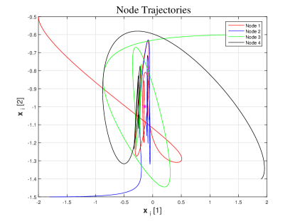
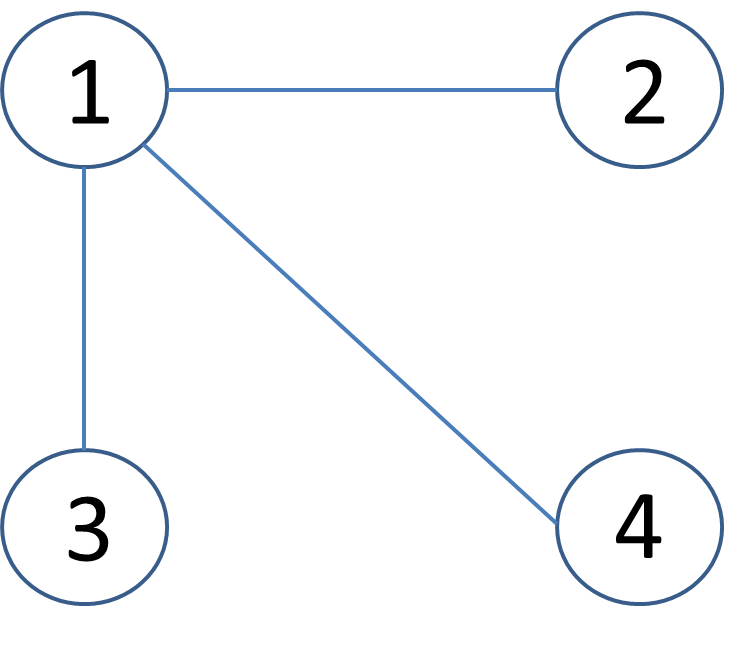
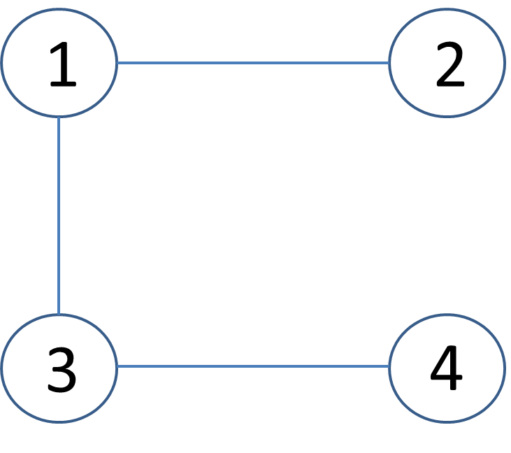
Then the equation has a unique least squares solution 𝐲=[0.14291]superscript𝐲superscriptdelimited-[]0.14291top\mathbf{y}^{\ast}=[-0.1429\ -1]^{\top}. Let the interaction graph 𝒢=(𝒱,)𝒢𝒱\mathcal{G}=(\mathcal{V},\mathcal{E}) be given in Figure 1. It can be noted that graph 𝒢𝒢\mathcal{G} is a path graph that satisfies Case [Path Graph](i) in Section 3.3. It is verified that there is no zero entry in any eigenvectors of 𝐋𝐋\mathbf{L} by calculating four eigenvectors as [0.50.50.50.5]superscriptdelimited-[]0.50.50.50.5top[-0.5\ -0.5\ -0.5\ -0.5]^{\top}, [0.27 0.650.270.65]superscriptdelimited-[]0.270.650.270.65top[0.27\ 0.65\ -0.27\ -0.65]^{\top}, [0.5 0.50.5 0.5]superscriptdelimited-[]0.50.50.50.5top[-0.5\ 0.5\ -0.5\ 0.5]^{\top} and [0.650.270.65 0.27]superscriptdelimited-[]0.650.270.650.27top[0.65\ -0.27\ -0.65\ 0.27]^{\top} corresponding to the eigenvalues 00, 0.590.590.59, 222 and 3.413.413.41, respectively. One can easily verify the condition of Theorem 1.(i) holds. Let 𝐱(0)=[20.51.81.5 1.80.6 1.91.4]𝐱0superscriptdelimited-[]20.51.81.51.80.61.91.4top\mathbf{x}(0)=[-2\ -0.5\ -1.8\ -1.5\ 1.8\ -0.6\ 1.9\ -1.4]^{\top}, 𝐯(0)=0𝐯00\mathbf{v}(0)=0 be the initial condition.

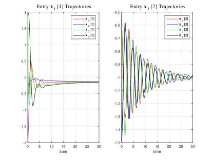
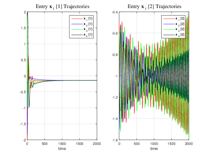
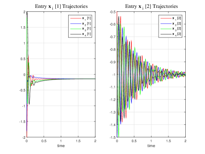
In Figure 2 we first plot the trajectories of the 𝐱i(t),i=1,2,3,4formulae-sequencesubscript𝐱𝑖𝑡𝑖1234\mathbf{x}_{i}(t),i=1,2,3,4 in 2superscript2\mathbb{R}^{2}. As we can see, all 𝐱i(t)subscript𝐱𝑖𝑡\mathbf{x}_{i}(t) converge to 𝐲superscript𝐲\mathbf{y}^{\ast}. A further confirmation from the two entries (𝐱i(t))[1]subscript𝐱𝑖𝑡delimited-[]1(\mathbf{x}_{i}(t))[1] and (𝐱i(t))[2]subscript𝐱𝑖𝑡delimited-[]2(\mathbf{x}_{i}(t))[2] is shown in Figure 3. The numerical result is consistent with Theorem 1.(i).
Refer to caption
Figure 1: A constant, undirected and connected graph with four nodes considered in Example 1 and Example 3.
Refer to caption
Figure 2: The trajectories of 𝐱𝐱\mathbf{x} over the graph in Figure 1. We can see that if the initial condition is [20.51.81.5 1.80.6 1.91.4]superscriptdelimited-[]20.51.81.51.80.61.91.4top[-2\ -0.5\ -1.8\ -1.5\ 1.8\ -0.6\ 1.9\ -1.4]^{\top}, it will converge to [0.14290.10.14290.10.14290.10.14290.1]superscriptdelimited-[]0.14290.10.14290.10.14290.10.14290.1top[-0.1429\ -0.1\ -0.1429\ -0.1\ -0.1429\ -0.1\ -0.1429\ -0.1]^{\top}.

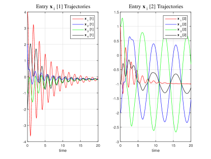
Example 2 Consider the linear equation (1) with the same 𝐇𝐇\mathbf{H} and 𝐳𝐳\mathbf{z} as in Example 1. Let the interaction graph 𝒢=(𝒱,)𝒢𝒱\mathcal{G}=(\mathcal{V},\mathcal{E}), which is a star graph studied in Section 3.3, be given in Figure 4. Let 𝐱(0)=[4 1 221 121]𝐱0superscriptdelimited-[]41221121top\mathbf{x}(0)=[4\ 1\ 2\ -2\ -1\ 1\ -2\ -1]^{\top}, 𝐯(0)=0𝐯00\mathbf{v}(0)=0 be the initial condition. As plotted in Figure 5, the first entries 𝐱i[1],i=1,2,3,4formulae-sequencesubscript𝐱𝑖delimited-[]1𝑖1234\mathbf{x}_{i}[1],i=1,2,3,4 converge to 𝐲[1]=0.1429superscript𝐲delimited-[]10.1429\mathbf{y}^{\ast}[1]=-0.1429. However, among the second entries only 𝐱1[2]subscript𝐱1delimited-[]2\mathbf{x}_{1}[2] converges to 𝐲[2]=1superscript𝐲delimited-[]21\mathbf{y}^{\ast}[2]=-1, while 𝐱2[2]subscript𝐱2delimited-[]2\mathbf{x}_{2}[2], 𝐱3[2]subscript𝐱3delimited-[]2\mathbf{x}_{3}[2] and 𝐱4[2]subscript𝐱4delimited-[]2\mathbf{x}_{4}[2] do not converge. In fact, the eigenvectors of the Laplacian for the given graph 𝒢𝒢\mathcal{G} are [0.50.50.50.5]superscriptdelimited-[]0.50.50.50.5top[-0.5\ -0.5\ -0.5\ -0.5]^{\top}, [00.640.11 0.75]superscriptdelimited-[]00.640.110.75top[0\ -0.64\ -0.11\ 0.75]^{\top}, [00.5 0.80.3]superscriptdelimited-[]00.50.80.3top[0\ -0.5\ 0.8\ -0.3]^{\top} and [0.87 0.29 0.29 0.29]superscriptdelimited-[]0.870.290.290.29top[-0.87\ 0.29\ 0.29\ 0.29]^{\top} corresponding to eigenvalues 00, 111, 111 and 444. For the eigenvector 𝜶=[00.640.11 0.75]𝜶superscriptdelimited-[]00.640.110.75top\bm{\alpha}=[0\ -0.64\ -0.11\ 0.75]^{\top} (or 𝜶=[00.5 0.80.3]𝜶superscriptdelimited-[]00.50.80.3top\bm{\alpha}=[0\ -0.5\ 0.8\ -0.3]^{\top}), there holds dim{𝐡i:𝜶[i]0}=dim{𝐡2,𝐡3,𝐡4}=1dimensionconditional-setsubscript𝐡𝑖𝜶delimited-[]𝑖0dimensionsubscript𝐡2subscript𝐡3subscript𝐡41\dim\{\mathbf{h}_{i}:\bm{\alpha}[i]\neq 0\}=\dim\{\mathbf{h}_{2},\mathbf{h}_{3},\mathbf{h}_{4}\}=1, leading to oscillating trajectories for 𝐱2[2]subscript𝐱2delimited-[]2\mathbf{x}_{2}[2], 𝐱3[2]subscript𝐱3delimited-[]2\mathbf{x}_{3}[2] and 𝐱4[2]subscript𝐱4delimited-[]2\mathbf{x}_{4}[2].

Refer to caption
Figure 3: The trajectories of 𝐱i[1]subscript𝐱𝑖delimited-[]1\mathbf{x}_{i}[1] and 𝐱i[2]subscript𝐱𝑖delimited-[]2\mathbf{x}_{i}[2] for i=1,2,3,4𝑖1234i=1,2,3,4 over the graph in Figure 1, which converge to 0.14290.1429-0.1429 and 11-1 respectively.
Refer to caption
Figure 4: A constant, undirected and connected graph with four nodes considered in Example 2 and Example 4.
Refer to caption
Figure 5: The trajectories of 𝐱i[1]subscript𝐱𝑖delimited-[]1\mathbf{x}_{i}[1] and 𝐱i[2]subscript𝐱𝑖delimited-[]2\mathbf{x}_{i}[2] for i=1,2,3,4𝑖1234i=1,2,3,4 over the graph in Figure 4. We can see that for all i𝑖i the first components 𝐱i[1]subscript𝐱𝑖delimited-[]1\mathbf{x}_{i}[1] converge to 0.14290.1429-0.1429, while only the second component 𝐱1[2]subscript𝐱1delimited-[]2\mathbf{x}_{1}[2] converges to 11-1.

4 Discrete-time Algorithm

In this section, we investigate the discrete-time analog of the flow (4). We index time as k=0,1,2,𝑘012k=0,1,2,\dots and propose the following algorithm:

𝐱(k+1)𝐱𝑘1\displaystyle\mathbf{x}(k+1) =𝐱(k)ϵ(𝐋𝐈m)𝐯(k)ϵU(𝐱(k))absent𝐱𝑘italic-ϵtensor-product𝐋subscript𝐈𝑚𝐯𝑘italic-ϵ𝑈𝐱𝑘\displaystyle=\mathbf{x}(k)-\epsilon(\mathbf{L}\otimes\mathbf{I}_{m})\mathbf{v}(k)-\epsilon\nabla U(\mathbf{x}(k)) (19)
𝐯(k+1)𝐯𝑘1\displaystyle\mathbf{v}(k+1) =𝐯(k)+ϵ(𝐋𝐈m)𝐱(k).absent𝐯𝑘italic-ϵtensor-product𝐋subscript𝐈𝑚𝐱𝑘\displaystyle=\mathbf{v}(k)+\epsilon(\mathbf{L}\otimes\mathbf{I}_{m})\mathbf{x}(k).

For [𝐱i(k)𝐯i(k)]superscriptdelimited-[]superscriptsubscript𝐱𝑖top𝑘superscriptsubscript𝐯𝑖top𝑘top[\mathbf{x}_{i}^{\top}(k)\ \mathbf{v}_{i}^{\top}(k)]^{\top} held by node i𝑖i, (19) gives

𝐱i(k+1)subscript𝐱𝑖𝑘1\displaystyle\mathbf{x}_{i}(k+1) =𝐱i(k)ϵj𝒩i(𝐯i(k)𝐯j(k))absentsubscript𝐱𝑖𝑘italic-ϵsubscript𝑗subscript𝒩𝑖subscript𝐯𝑖𝑘subscript𝐯𝑗𝑘\displaystyle=\mathbf{x}_{i}(k)-\epsilon\sum_{j\in\mathcal{N}_{i}}(\mathbf{v}_{i}(k)-\mathbf{v}_{j}(k))
ϵ(𝐡i𝐡i𝐱i(k)zi𝐡i)italic-ϵsubscript𝐡𝑖superscriptsubscript𝐡𝑖topsubscript𝐱𝑖𝑘subscript𝑧𝑖subscript𝐡𝑖\displaystyle-\epsilon(\mathbf{h}_{i}\mathbf{h}_{i}^{\top}\mathbf{x}_{i}(k)-z_{i}\mathbf{h}_{i})
𝐯i(k+1)subscript𝐯𝑖𝑘1\displaystyle\mathbf{v}_{i}(k+1) =𝐯i(k)+ϵj𝒩i(𝐱i(k)𝐯i(k)).absentsubscript𝐯𝑖𝑘italic-ϵsubscript𝑗subscript𝒩𝑖subscript𝐱𝑖𝑘subscript𝐯𝑖𝑘\displaystyle=\mathbf{v}_{i}(k)+\epsilon\sum_{j\in\mathcal{N}_{i}}(\mathbf{x}_{i}(k)-\mathbf{v}_{i}(k)).

Therefore, the algorithm (19) inherits the same distributed structure as the flow (4). Note that (19) is an Euler approximation of (4). However, since dynamical system (4) does not have all its modes exponentially stable, we cannot immediately conclude that for a sufficiently small ϵitalic-ϵ\epsilon, the solution to (19) will converge to the same consensus as (4).

4.1 Convergence Result

Recall that 𝐲superscript𝐲\mathbf{y}^{\ast} is the unique least squares solution of (1) and denote

𝐌=[𝐇~(𝐋𝐈m)𝐋𝐈m0].𝐌matrix~𝐇tensor-product𝐋subscript𝐈𝑚tensor-product𝐋subscript𝐈𝑚0\mathbf{M}=\begin{bmatrix}-\tilde{\mathbf{H}}&-(\mathbf{L}\otimes\mathbf{I}_{m})\\ \mathbf{L}\otimes\mathbf{I}_{m}&0\end{bmatrix}.

The following result holds.

Theorem 2

Suppose span{𝐡i:𝛂[i]0}=mspan:subscript𝐡𝑖𝛂delimited-[]𝑖0superscript𝑚\operatorname{span}\{\mathbf{h}_{i}:\bm{\alpha}[i]\neq 0\}=\mathbb{R}^{m} for all the eigenvectors 𝛂=[𝛂[1]𝛂[N]]N𝛂superscriptdelimited-[]𝛂delimited-[]1𝛂delimited-[]𝑁topsuperscript𝑁\bm{\alpha}=\big{[}\bm{\alpha}[1]\ \dots\ \bm{\alpha}[N]\big{]}^{\top}\in\mathbb{C}^{N} of 𝐋𝐋\mathbf{L}. Then there exists a positive constant ϵsuperscriptitalic-ϵ\epsilon^{\ast} such that

  1. (i)

    If 0<ϵ<ϵ0italic-ϵsuperscriptitalic-ϵ0<\epsilon<\epsilon^{\ast}, then along (19) we have

    limk𝐱i(k)=y,i=1,,Nformulae-sequencesubscript𝑘subscript𝐱𝑖𝑘superscript𝑦𝑖1𝑁\lim_{k\to\infty}\mathbf{x}_{i}(k)=y^{\ast},i=1,\dots,N

    which converge exponentially for all i𝑖i. In this case 𝐯(k)𝐯𝑘\mathbf{v}(k) continues to converge to a constant.

  2. (ii)

    If ϵ>ϵitalic-ϵsuperscriptitalic-ϵ\epsilon>\epsilon^{\ast}, then along (19) there exist initial values 𝐱(0)𝐱0\mathbf{x}(0) and 𝐯(0)𝐯0\mathbf{v}(0) under which [𝐱(k)𝐯(k)]superscriptdelimited-[]𝐱superscript𝑘top𝐯superscript𝑘toptop[\mathbf{x}(k)^{\top}\ \mathbf{v}(k)^{\top}]^{\top} diverges.

Define σ(𝐌)σ(𝐌)superscript𝜎𝐌𝜎𝐌\sigma^{\ast}(\mathbf{M})\subset\sigma(\mathbf{M}) by σ(𝐌):={λσ(𝐌):(λ)0}assignsuperscript𝜎𝐌conditional-set𝜆𝜎𝐌𝜆0\sigma^{\ast}(\mathbf{M}):=\{\lambda\in\sigma(\mathbf{M}):\Re(\lambda)\neq 0\}. Then ϵ=minλσ(𝐌)[2(λ)|λ|2]superscriptitalic-ϵsubscript𝜆superscript𝜎𝐌2𝜆superscript𝜆2\epsilon^{\ast}=\min\limits_{\lambda\in\sigma^{\ast}(\mathbf{M})}\big{[}-\frac{2\Re(\lambda)}{|\lambda|^{2}}\big{]}.

Proof. Let 𝐱=𝟏𝐲superscript𝐱tensor-product1superscript𝐲\mathbf{x}^{\ast}=\mathbf{1}\otimes\mathbf{y}^{\ast} and 𝐯superscript𝐯\mathbf{v}^{\ast} satisfy U(𝐱)+(𝐋𝐈m)𝐯=0𝑈superscript𝐱tensor-product𝐋subscript𝐈𝑚superscript𝐯0\nabla U(\mathbf{x}^{\ast})+(\mathbf{L}\otimes\mathbf{I}_{m})\mathbf{v}^{\ast}=0. We continue to use the change of variables defined by 𝐱^(k)=𝐱(k)𝐱^𝐱𝑘𝐱𝑘superscript𝐱\hat{\mathbf{x}}(k)=\mathbf{x}(k)-\mathbf{x}^{\ast} and 𝐯^(k)=𝐯(k)𝐯^𝐯𝑘𝐯𝑘superscript𝐯\hat{\mathbf{v}}(k)=\mathbf{v}(k)-\mathbf{v}^{\ast} so that the equilibrium of (19) is shifted. We have

𝐱^(k+1)^𝐱𝑘1\displaystyle\hat{\mathbf{x}}(k+1) =𝐱^(k)ϵ(𝐋𝐋m)𝐯^(k)ϵ𝐇~x^(k)absent^𝐱𝑘italic-ϵtensor-product𝐋subscript𝐋𝑚^𝐯𝑘italic-ϵ~𝐇^𝑥𝑘\displaystyle=\hat{\mathbf{x}}(k)-\epsilon(\mathbf{L}\otimes\mathbf{L}_{m})\hat{\mathbf{v}}(k)-\epsilon\tilde{\mathbf{H}}\hat{x}(k)
𝐯^(k+1)^𝐯𝑘1\displaystyle\hat{\mathbf{v}}(k+1) =𝐯^(k)+ϵ(𝐋𝐈m)𝐱^(k),absent^𝐯𝑘italic-ϵtensor-product𝐋subscript𝐈𝑚^𝐱𝑘\displaystyle=\hat{\mathbf{v}}(k)+\epsilon(\mathbf{L}\otimes\mathbf{I}_{m})\hat{\mathbf{x}}(k),

or equivalently,

[𝐱^(k+1)𝐯^(k+1)]=(𝐈+ϵ𝐌)[𝐱^(k)𝐯^(k)].matrix^𝐱𝑘1^𝐯𝑘1𝐈italic-ϵ𝐌matrix^𝐱𝑘^𝐯𝑘\begin{bmatrix}\hat{\mathbf{x}}(k+1)\\ \hat{\mathbf{v}}(k+1)\end{bmatrix}=(\mathbf{I}+\epsilon\mathbf{M})\begin{bmatrix}\hat{\mathbf{x}}(k)\\ \hat{\mathbf{v}}(k)\end{bmatrix}.

Now note that the proof of Theorem 1 in effect proves certain properties of the continuous time equation

[𝐱^˙𝐯^˙]=𝐌[𝐱^𝐯^].matrix˙^𝐱˙^𝐯𝐌matrix^𝐱^𝐯\begin{bmatrix}\dot{\hat{\mathbf{x}}}\\ \dot{\hat{\mathbf{v}}}\end{bmatrix}=\mathbf{M}\begin{bmatrix}\hat{\mathbf{x}}\\ \hat{\mathbf{v}}\end{bmatrix}.

In fact, from the convergence properties of [𝐱^(t)𝐯^(t)]superscriptdelimited-[]^𝐱superscript𝑡top^𝐯superscript𝑡toptop[\hat{\mathbf{x}}(t)^{\top}\ \hat{\mathbf{v}}(t)^{\top}]^{\top} that are established in the proof of Theorem 1, we can conclude the following for 𝐌𝐌\mathbf{M} from basic linear system theory when span{𝐡i:𝜶[i]0}=mspan:subscript𝐡𝑖𝜶delimited-[]𝑖0superscript𝑚\operatorname{span}\{\mathbf{h}_{i}:\bm{\alpha}[i]\neq 0\}=\mathbb{R}^{m} for all eigenvalues 𝜶=[𝜶[1]α[N]]𝜶superscriptdelimited-[]𝜶delimited-[]1𝛼delimited-[]𝑁top\bm{\alpha}=\big{[}\bm{\alpha}[1]\ \dots\ \alpha[N]\big{]}^{\top} of 𝐋𝐋\mathbf{L}:

(a) (λ)<0𝜆0\Re(\lambda)<0 for all λσ(𝐌)𝜆𝜎𝐌\lambda\in\sigma(\mathbf{M}) with λ0𝜆0\lambda\neq 0;

(b) Zero is an eigenvalue of 𝐌𝐌\mathbf{M} with equal algebraic and geometric multiplicity;

(c) The zero eigenspace of 𝐌𝐌\mathbf{M} is given by {[𝐱𝐯]:(𝐋𝐈m)𝐱=0,𝐇~𝐱+(𝐋𝐈m)𝐯=0}conditional-setsuperscriptdelimited-[]superscript𝐱topsuperscript𝐯toptopformulae-sequencetensor-product𝐋subscript𝐈𝑚𝐱0~𝐇𝐱tensor-product𝐋subscript𝐈𝑚𝐯0\{[\mathbf{x}^{\top}\ \mathbf{v}^{\top}]^{\top}:(\mathbf{L}\otimes\mathbf{I}_{m})\mathbf{x}=0,\tilde{\mathbf{H}}\mathbf{x}+(\mathbf{L}\otimes\mathbf{I}_{m})\mathbf{v}=0\}.

It is straightforward that

σ(𝐈+ϵ𝐌)={1+ϵλ:λσ(𝐌)}.𝜎𝐈italic-ϵ𝐌conditional-set1italic-ϵ𝜆𝜆𝜎𝐌\sigma(\mathbf{I}+\epsilon\mathbf{M})=\{1+\epsilon\lambda:\lambda\in\sigma(\mathbf{M})\}.

and then the eigenvalues of M𝑀M, coupled with the continuity of σ(1+ϵ𝐌)𝜎1italic-ϵ𝐌\sigma(1+\epsilon\mathbf{M}) as a function of ϵitalic-ϵ\epsilon, imply that there exists ϵ>0superscriptitalic-ϵ0\epsilon^{\ast}>0 such that

(i) when 0<ϵ<ϵ0italic-ϵsuperscriptitalic-ϵ0<\epsilon<\epsilon^{\ast}, there hold

  • |λ|<1𝜆1|\lambda|<1 for all λσ(1+ϵ𝐌)𝜆𝜎1italic-ϵ𝐌\lambda\in\sigma(1+\epsilon\mathbf{M}) with λ1𝜆1\lambda\neq 1;

  • 111 is an eigenvalue of 1+ϵ𝐌1italic-ϵ𝐌1+\epsilon\mathbf{M} with equal algebraic and geometric multiplicity.

Moreover, the eigenspace of 1+ϵ𝐌1italic-ϵ𝐌1+\epsilon\mathbf{M} corresponding to eigenvalue one is the same as the eigenspace of 𝐌𝐌\mathbf{M} corresponding to eigenvalue zero.

Consequently, [𝐱^(k)𝐯^(k)]superscriptdelimited-[]^𝐱superscript𝑘top^𝐯superscript𝑘toptop[\hat{\mathbf{x}}(k)^{\top}\ \hat{\mathbf{v}}(k)^{\top}]^{\top} converges to a vector in 2Nmsuperscript2𝑁𝑚\mathbb{R}^{2Nm}, which implies, together with the structure of the eigenspace for the eigenvalue 111, the desired convergence for [𝐱(k)𝐯(k)]superscriptdelimited-[]𝐱superscript𝑘top𝐯superscript𝑘toptop[\mathbf{x}(k)^{\top}\ \mathbf{v}(k)^{\top}]^{\top}.

(ii) when ϵ>ϵitalic-ϵsuperscriptitalic-ϵ\epsilon>\epsilon^{\ast}, there exists λσ(1+ϵ𝐌)𝜆𝜎1italic-ϵ𝐌\lambda\in\sigma(1+\epsilon\mathbf{M}) with |λ|>1𝜆1|\lambda|>1. Therefore, [𝐱^(k)𝐯^(k)]superscriptdelimited-[]^𝐱superscript𝑘top^𝐯superscript𝑘toptop[\hat{\mathbf{x}}(k)^{\top}\ \hat{\mathbf{v}}(k)^{\top}]^{\top} will diverge for certain initial values, so in turn [𝐱(k)𝐯(k)]superscriptdelimited-[]𝐱superscript𝑘top𝐯superscript𝑘toptop[\mathbf{x}(k)^{\top}\ \mathbf{v}(k)^{\top}]^{\top} will also diverge.

Finally, we compute the value of ϵsuperscriptitalic-ϵ\epsilon^{\ast}. Consider the following set of functions of ϵitalic-ϵ\epsilon: σλ(ϵ)=1+ϵ((λ)+ı(λ))subscript𝜎𝜆italic-ϵ1italic-ϵ𝜆italic-ı𝜆\sigma_{\lambda}(\epsilon)=1+\epsilon(\Re(\lambda)+\imath\Im(\lambda)) with λσ(𝐌)𝜆superscript𝜎𝐌\lambda\in\sigma^{\ast}(\mathbf{M}). According to the definition of ϵsuperscriptitalic-ϵ\epsilon^{\ast}, ϵsuperscriptitalic-ϵ\epsilon^{\ast} must be the smallest ϵλsubscriptsuperscriptitalic-ϵ𝜆\epsilon^{\ast}_{\lambda} for which

|σλ(ϵλ)|=(ϵλ(λ)+1)2+(ϵλ(λ))2=1.subscript𝜎𝜆subscriptsuperscriptitalic-ϵ𝜆superscriptsuperscriptsubscriptitalic-ϵ𝜆𝜆12superscriptsuperscriptsubscriptitalic-ϵ𝜆𝜆21|\sigma_{\lambda}(\epsilon^{\ast}_{\lambda})|=\sqrt{(\epsilon_{\lambda}^{\ast}\Re(\lambda)+1)^{2}+(\epsilon_{\lambda}^{\ast}\Im(\lambda))^{2}}=1.

Therefore, we conclude ϵ=minλσ(𝐌)[2(λ)|λ|2]superscriptitalic-ϵsubscript𝜆superscript𝜎𝐌2𝜆superscript𝜆2\epsilon^{\ast}=\min\limits_{\lambda\in\sigma^{\ast}(\mathbf{M})}\big{[}-\frac{2\Re(\lambda)}{|\lambda|^{2}}\big{]}.

We have now completed the proof of Theorem 2.

When ϵ=ϵitalic-ϵsuperscriptitalic-ϵ\epsilon=\epsilon^{\ast}, of course 1+ϵ𝐌1superscriptitalic-ϵ𝐌1+\epsilon^{\ast}\mathbf{M} might have complex eigenvalues on the unit circle, leading to the possibility of periodic trajectories for [𝐱(k)𝐯(k)]superscriptdelimited-[]𝐱superscript𝑘top𝐯superscript𝑘toptop[\mathbf{x}(k)^{\top}\ \mathbf{v}(k)^{\top}]^{\top}. Based on Theorem 1. (ii), one might also expect that periodic trajectories could occur in discrete time when the dimensionality condition is fulfilled. In contrast however, we have the following result.

Theorem 3

If dim(span{𝐡i:𝛂[i]0})<mdimensionspan:subscript𝐡𝑖𝛂delimited-[]𝑖0𝑚\dim(\operatorname{span}\{\mathbf{h}_{i}:\bm{\alpha}[i]\neq 0\})<m, then for any ϵ>0italic-ϵ0\epsilon>0, there always exist trajectories 𝐱(k)𝐱𝑘\mathbf{x}(k) for the algorithm (19) that diverge as k𝑘k tends to infinity.

Proof. From the proof of Theorem 1 we see that 𝐌𝐌\mathbf{M} will have eigenvalues on the imaginary axis with dim(span{𝐡i:𝜶[i]0})<mdimensionspan:subscript𝐡𝑖𝜶delimited-[]𝑖0𝑚\dim(\operatorname{span}\{\mathbf{h}_{i}:\bm{\alpha}[i]\neq 0\})<m. Such 𝐌𝐌\mathbf{M} generate eigenvalues λσ(1+ϵ𝐌)𝜆𝜎1italic-ϵ𝐌\lambda\in\sigma(1+\epsilon\mathbf{M}) with |λ|>1𝜆1|\lambda|>1. Therefore, for any ϵ>0italic-ϵ0\epsilon>0 and for all but a thin set of initial values, the trajectory [𝐱(k)𝐯(k)]superscriptdelimited-[]𝐱superscript𝑘top𝐯superscript𝑘toptop[\mathbf{x}(k)^{\top}\ \mathbf{v}(k)^{\top}]^{\top} diverges. This proves the desired result. \square
Refer to caption
Figure 6: The trajectories of 𝐱i[1]subscript𝐱𝑖delimited-[]1\mathbf{x}_{i}[1] and 𝐱i[2]subscript𝐱𝑖delimited-[]2\mathbf{x}_{i}[2] for i=1,2,3,4𝑖1234i=1,2,3,4 over the graph in Figure 1 when ϵ=0.03italic-ϵ0.03\epsilon=0.03. We see that 𝐱i(t)subscript𝐱𝑖𝑡\mathbf{x}_{i}(t) converges for each i𝑖i to the least squares solution [0.14291]superscriptdelimited-[]0.14291top[-0.1429\ -1]^{\top}.
Refer to caption
Figure 7: The trajectories of 𝐱i[2]subscript𝐱𝑖delimited-[]2\mathbf{x}_{i}[2] for i=1,2,3,4𝑖1234i=1,2,3,4 diverge fast over the graph in Figure 1 when ϵ=0.04italic-ϵ0.04\epsilon=0.04.

4.2 Numerical Examples

We now provide several numerical illustrations to the results stated in Theorem 2 and Theorem 3.

Example 3. Consider a linear equation in the form of (1) where 𝐲2𝐲superscript2\mathbf{y}\in\mathbb{R}^{2}, and

𝐇=[01302010],𝐳=[1022].formulae-sequence𝐇matrix01302010𝐳matrix1022\mathbf{H}=\begin{bmatrix}0&1\\ 3&0\\ 2&0\\ 1&0\\ \end{bmatrix},\quad\mathbf{z}=\begin{bmatrix}-1\\ 0\\ -2\\ 2\end{bmatrix}.

It has a unique least squares solution 𝐲=[0.14291]superscript𝐲superscriptdelimited-[]0.14291top\mathbf{y}^{\ast}=[-0.1429\ -1]^{\top}. Let 𝒢=(𝒱,)𝒢𝒱\mathcal{G}=(\mathcal{V},\mathcal{E}) be the graph given in Figure 1. By simple computation, ϵ=0.0362superscriptitalic-ϵ0.0362\epsilon^{\ast}=0.0362. We have noted in Example 1 that graph 𝒢𝒢\mathcal{G} satisfies the condition that span{𝐡i:𝜶[i]0}=mspan:subscript𝐡𝑖𝜶delimited-[]𝑖0superscript𝑚\operatorname{span}\{\mathbf{h}_{i}:\bm{\alpha}[i]\neq 0\}=\mathbb{R}^{m} for all eigenvalues 𝜶=[𝜶[1]𝜶[N]]𝜶superscriptdelimited-[]𝜶delimited-[]1𝜶delimited-[]𝑁top\bm{\alpha}=\big{[}\bm{\alpha}[1]\ \dots\ \bm{\alpha}[N]\big{]}^{\top} of 𝐋𝐋\mathbf{L}. We first set ϵ=0.03<ϵitalic-ϵ0.03superscriptitalic-ϵ\epsilon=0.03<\epsilon^{\ast} and plot the trajectories in Figure 6. We can see that they all converge to the solution 𝐲superscript𝐲\mathbf{y}^{\ast}. Next we set ϵ=0.04>ϵitalic-ϵ0.04superscriptitalic-ϵ\epsilon=0.04>\epsilon^{\ast} and plot the trajectories in Figure 7. It is apparent that the trajectories of 𝐱i[2]subscript𝐱𝑖delimited-[]2\mathbf{x}_{i}[2] for i=1,2,3,4𝑖1234i=1,2,3,4 diverge. This example is consistent with Theorem 2.

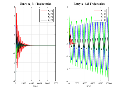
Example 4. Consider the linear equation (1) with the same 𝐇𝐇\mathbf{H}, 𝐳𝐳\mathbf{z} and 𝐲superscript𝐲\mathbf{y}^{\ast} as in Example 3. Let 𝒢=(𝒱,)𝒢𝒱\mathcal{G}=(\mathcal{V},\mathcal{E}) be the graph in Figure 4 satisfying the condition of Theorem 3, as noted when we explored Example 2. Let ϵ=0.01italic-ϵ0.01\epsilon=0.01. We plot the trajectories of 𝐱i[1]subscript𝐱𝑖delimited-[]1\mathbf{x}_{i}[1] and 𝐱i[2]subscript𝐱𝑖delimited-[]2\mathbf{x}_{i}[2] for i=1,2,3,4𝑖1234i=1,2,3,4 in Figure 8. It is evident that the trajectories of 𝐱2[2]subscript𝐱2delimited-[]2\mathbf{x}_{2}[2], 𝐱3[2]subscript𝐱3delimited-[]2\mathbf{x}_{3}[2] and 𝐱4[2]subscript𝐱4delimited-[]2\mathbf{x}_{4}[2] diverge; this is consistent with Theorem 3.
Refer to caption
Figure 8: The trajectories of 𝐱i[1]subscript𝐱𝑖delimited-[]1\mathbf{x}_{i}[1] and 𝐱i[2]subscript𝐱𝑖delimited-[]2\mathbf{x}_{i}[2] for i=1,2,3,4𝑖1234i=1,2,3,4 over the graph in Figure 4 when ϵ=0.01italic-ϵ0.01\epsilon=0.01. We see that the trajectories of 𝐱2[2]subscript𝐱2delimited-[]2\mathbf{x}_{2}[2], 𝐱3[2]subscript𝐱3delimited-[]2\mathbf{x}_{3}[2] and 𝐱4[2]subscript𝐱4delimited-[]2\mathbf{x}_{4}[2] diverge.

When ϵ=0.5italic-ϵ0.5\epsilon=0.5, all trajectories over both graphs in Figure 1 and Figure 4 fail to converge.

5 Further Discussions

In this section, we provide some further results and investigations regarding the least squares residual vector, alternative state expansion methods, and the influence of switching network structures.

5.1 Residual vector

The residual vector of (1) is defined as

𝐞=𝐇𝐲𝐳superscript𝐞superscript𝐇𝐲𝐳\mathbf{e}^{\ast}=\mathbf{H}\mathbf{y}^{\ast}-\mathbf{z}

with 𝐲superscript𝐲\mathbf{y}^{\ast} being the least squares solution. Since each node i𝑖i holds the information of 𝐡isubscript𝐡𝑖\mathbf{h}_{i} and 𝐳isubscript𝐳𝑖\mathbf{z}_{i}, the i𝑖i-th component eisuperscriptsubscript𝑒𝑖e_{i}^{\ast} of the residual vector 𝐞superscript𝐞\mathbf{e}^{\ast} can be obtained by node i𝑖i after running the continuous-time flow (4) by ei=limt(𝐡i𝐱i(t)zi)superscriptsubscript𝑒𝑖subscript𝑡superscriptsubscript𝐡𝑖topsubscript𝐱𝑖𝑡subscript𝑧𝑖e_{i}^{\ast}=\lim\limits_{t\to\infty}(\mathbf{h}_{i}^{\top}\mathbf{x}_{i}(t)-z_{i}) if the condition of Theorem 1.(i) is satisfied. Therefore, after executions of the presented continuous or discrete algorithms, another distributed agreement algorithm, e.g., [31], can be applied to the network so that all nodes can learn the entire residual vector 𝐞superscript𝐞\mathbf{e}^{\ast}.

5.2 State Expansion

Consider a linear equation with respect to 𝐲¯¯𝐲\bar{\mathbf{y}}:

𝐇¯𝐲¯=𝐳¯¯𝐇¯𝐲¯𝐳\bar{\mathbf{H}}\bar{\mathbf{y}}=\bar{\mathbf{z}} (20)

where

𝐇¯=[𝐇𝐈N0𝐇]¯𝐇matrix𝐇subscript𝐈𝑁0superscript𝐇top\bar{\mathbf{H}}=\begin{bmatrix}\mathbf{H}&-\mathbf{I}_{N}\\ 0&\mathbf{H}^{\top}\end{bmatrix}

and 𝐳¯=[𝐳 0]¯𝐳superscriptdelimited-[]superscript𝐳top 0top\bar{\mathbf{z}}=[\mathbf{z}^{\top}\ 0]^{\top}. It is known and easily checked that if 𝐇𝐇\mathbf{H} has full column rank, (20) has a unique exact solution in the form of 𝐲¯=[𝐲𝐞]superscript¯𝐲superscriptdelimited-[]superscript𝐲absenttopsuperscript𝐞absenttoptop\bar{\mathbf{y}}^{\ast}=[\mathbf{y}^{\ast\top}\ \mathbf{e}^{\ast\top}]^{\top} where 𝐲superscript𝐲\mathbf{y}^{\ast} is the least squares solution of (1) and 𝐞superscript𝐞\mathbf{e}^{\ast} is the residual vector. Therefore, distributed algorithms presented in [25, 26, 20, 21, 22, 3, 33] for solving linear algebraic equations with exact solutions can be used to solve (20), which in turn gives us the least squares solution of (1).

Such algorithms admit simple first-order structure even working for time-varying networks, e.g., [26, 33]. However, in order to construct (20), we have to add some additional m𝑚m nodes to the network which have access to the columns of 𝐇𝐇\mathbf{H}, imposing a much more restricted assumption on the node information structure.

5.3 Switching Networks

We have known that the network flow (4) defines a linear time-invariant (LTI) system since the network is fixed. However, many networks from real-world applications are time-varying, e.g., [29, 2]. If the network underlying (4) is indeed switching, (4) will in turn induce linear time-varying (LTV) dynamics. Since (4) is only marginally stable regardless of choice of network, generally speaking, existing theories for the stability of LTV systems cannot be directly applied. In this section, we use numerical examples to study the asymptotic properties of (4) under switching networks.

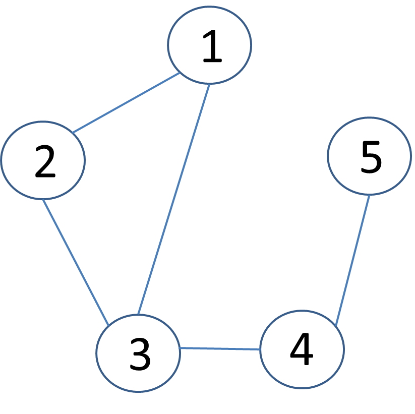
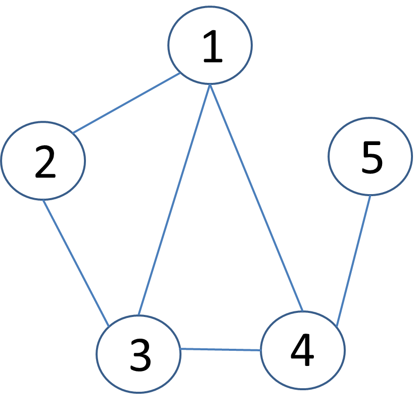
We now define precisely networks with switching interaction structures. Let 𝒬𝒬\mathcal{Q} be the set containing all graphs with node set 𝒱𝒱\mathcal{V}. Let 𝒬𝒬superscript𝒬𝒬\mathcal{Q}^{\ast}\subset\mathcal{Q} and introduce a piecewise constant mapping 𝒢σ():0𝒬:subscript𝒢𝜎superscriptabsent0superscript𝒬\mathcal{G}_{\sigma(\cdot)}:\mathbb{R}^{\geq 0}\to\mathcal{Q}^{\ast}. Then 𝒢σ(t)=(𝒱,σ(t))subscript𝒢𝜎𝑡𝒱subscript𝜎𝑡\mathcal{G}_{\sigma(t)}=(\mathcal{V},\mathcal{E}_{\sigma(t)}) represents the network topology at time t𝑡t. We consider a network with 555 nodes indexed in 𝒱={1,2,3,4,5}𝒱12345\mathcal{V}=\{1,2,3,4,5\}. We also let 𝒬={𝒢1,𝒢2}superscript𝒬subscript𝒢1subscript𝒢2\mathcal{Q}^{\ast}=\{\mathcal{G}_{1},\mathcal{G}_{2}\} where 𝒢1subscript𝒢1\mathcal{G}_{1}, 𝒢2subscript𝒢2\mathcal{G}_{2} are as shown in Fig. 9, Fig. 10, respectively. Denote the Laplacian of 𝒢1subscript𝒢1\mathcal{G}_{1}, 𝒢2subscript𝒢2\mathcal{G}_{2} by 𝐋1subscript𝐋1\mathbf{L}_{1}, 𝐋2subscript𝐋2\mathbf{L}_{2}. We know from direct calculation that 𝜶={1,2,3,4,5}subscript𝜶12345\mathcal{I}_{\bm{\alpha}}=\{1,2,3,4,5\} or 𝜶={1,2}subscript𝜶12\mathcal{I}_{\bm{\alpha}}=\{1,2\} for 𝜶𝒮𝐋1𝜶subscript𝒮subscript𝐋1\bm{\alpha}\in\mathcal{S}_{\mathbf{L}_{1}} and 𝜶={1,2,3,4,5}subscript𝜶12345\mathcal{I}_{\bm{\alpha}}=\{1,2,3,4,5\} or 𝜶={1,3}subscript𝜶13\mathcal{I}_{\bm{\alpha}}=\{1,3\} for 𝜶𝒮𝐋2𝜶subscript𝒮subscript𝐋2\bm{\alpha}\in\mathcal{S}_{\mathbf{L}_{2}}. For simplicity we assume that the switchings in the graph signal are periodic, as indicated in the following:

𝒢σ(t)={𝒢1,t[Tl,T(l+1)),l=0,2,4,𝒢2,t[Tl,T(l+1)),l=1,3,5,\mathcal{G}_{\sigma(t)}=\left\{\begin{aligned} &\mathcal{G}_{1},\ t\in\big{[}Tl,T(l+1)\big{)},l=0,2,4,\dots\\ &\mathcal{G}_{2},\ t\in\big{[}Tl,T(l+1)\big{)},l=1,3,5,\dots\\ \end{aligned}\right.

where T𝑇T\in\mathbb{R} is the period.

Refer to caption
Figure 9: Graph 𝒢1subscript𝒢1\mathcal{G}_{1} with five nodes.
Refer to caption
Figure 10: Graph 𝒢2subscript𝒢2\mathcal{G}_{2} with five nodes.

5.3.1 Switching of Converging Networks

First of all, we study the case where the graphs in 𝒬superscript𝒬\mathcal{Q}^{\ast} satisfy the condition stated in Theorem 1.(i), i.e., each individual graph in the switching graph signals will be able to produce trajectories for all 𝐱i(t)subscript𝐱𝑖𝑡\mathbf{x}_{i}(t) converging to the least square solutions in the absence of switching.
Refer to caption
(a) T=100
Refer to caption
(b) T=10
Refer to caption
(c) T=1
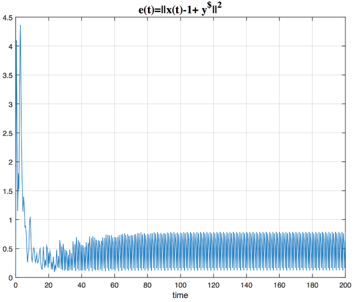
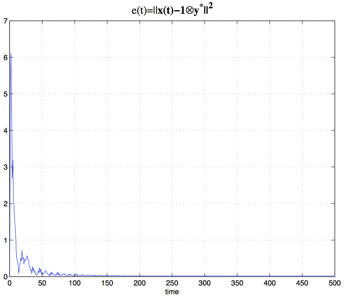
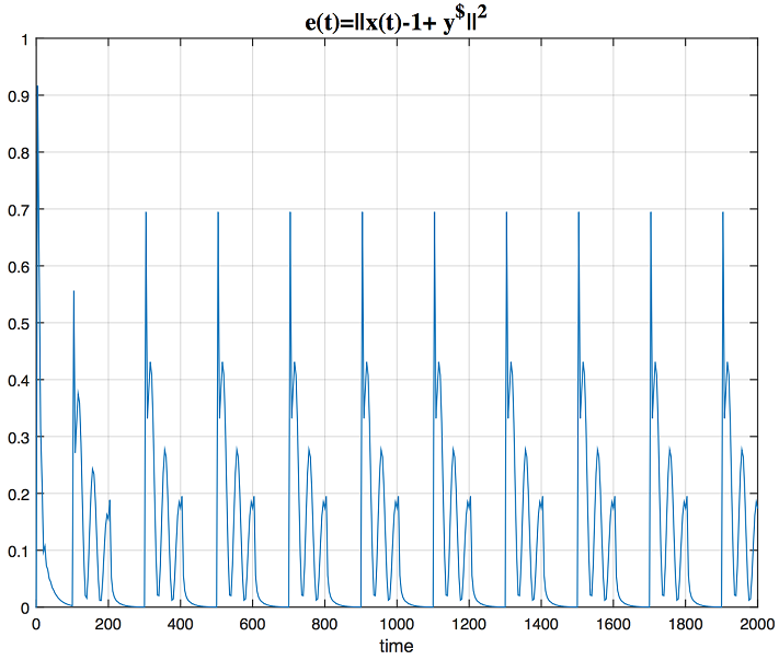
Figure 11: The trajectories of e(t)=𝐱(t)𝟏5𝐲2𝑒𝑡superscriptnorm𝐱𝑡tensor-productsubscript15superscript𝐲2e(t)=\|\mathbf{x}(t)-\mathbf{1}_{5}\otimes\mathbf{y}^{\ast}\|^{2} for i=1,2,3,4,5𝑖12345i=1,2,3,4,5 when (a) T=100𝑇100T=100, (b) T=10𝑇10T=10, (c) T=1𝑇1T=1.
Refer to caption
(a) T=100
Refer to caption
(b) T=10
Refer to caption
(c) T=1
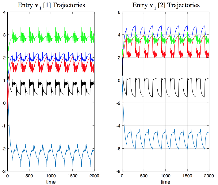
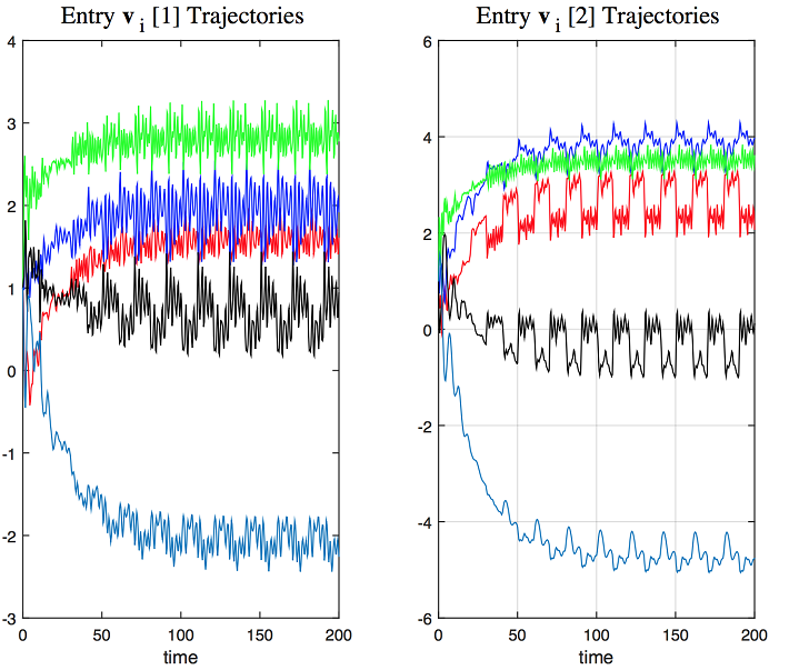
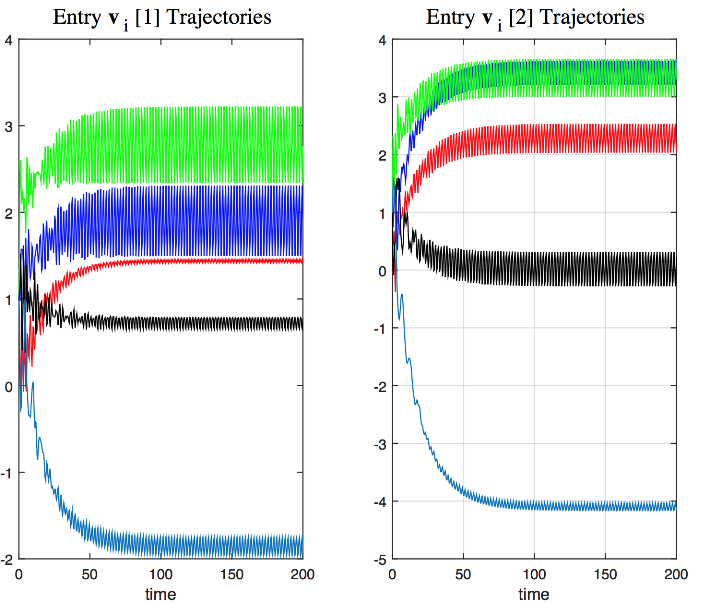
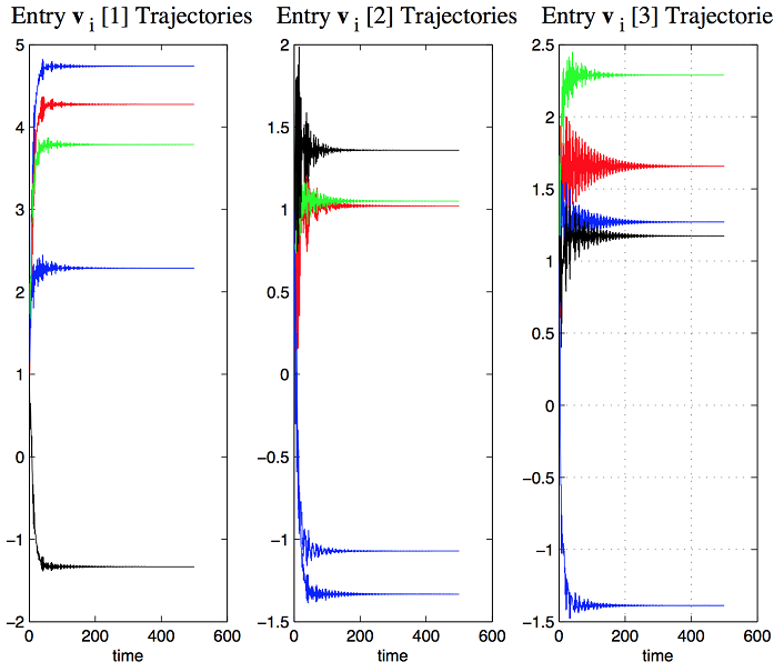
Figure 12: The trajectories of (𝐯i(t))[1]subscript𝐯𝑖𝑡delimited-[]1(\mathbf{v}_{i}(t))[1] and (𝐯i(t))[2]subscript𝐯𝑖𝑡delimited-[]2(\mathbf{v}_{i}(t))[2] for i=1,2,3,4,5𝑖12345i=1,2,3,4,5 when (a) T=100𝑇100T=100, (b) T=10𝑇10T=10, (c) T=1𝑇1T=1.

Example 5. Consider a linear equation (1) with

𝐇=[3213111.542.54],𝐳=[2152.50.25].formulae-sequence𝐇matrix3213111.542.54𝐳matrix2152.50.25\mathbf{H}=\begin{bmatrix}3&2\\ 1&-3\\ 1&1\\ -1.5&4\\ 2.5&4\end{bmatrix},\ \mathbf{z}=\begin{bmatrix}2\\ 1\\ 5\\ -2.5\\ 0.25\end{bmatrix}.

Then it has a unique least squares solution as 𝐲=[0.930.23]superscript𝐲superscriptdelimited-[]0.930.23top\mathbf{y}^{\ast}=[0.93\ -0.23]^{\top}. It can be verified that the condition of Theorem 1.(i) is met for both 𝒢1subscript𝒢1\mathcal{G}_{1} and 𝒢2subscript𝒢2\mathcal{G}_{2}. Let 𝐱(0)=[10.5 1.30.8 0.7 0.6 0.71.40.5 1]𝐱0superscriptdelimited-[]10.51.30.80.70.60.71.40.51top\mathbf{x}(0)=[1\ -0.5\ 1.3\ -0.8\ 0.7\ 0.6\ 0.7\ -1.4\ -0.5\ 1]^{\top}, 𝐯(0)=𝟏10𝐯0subscript110\mathbf{v}(0)=\mathbf{1}_{10} be the initial condition. In Figure 11, we plot the trajectories of

e(t)=𝐱(t)𝟏5𝐲2𝑒𝑡superscriptnorm𝐱𝑡tensor-productsubscript15superscript𝐲2e(t)=\|\mathbf{x}(t)-\mathbf{1}_{5}\otimes\mathbf{y}^{\ast}\|^{2}

for T=100,10,1𝑇100101T=100,10,1, respectively. We find that e(t)𝑒𝑡e(t) oscillates at the same frequency as 𝒢σ(t)subscript𝒢𝜎𝑡\mathcal{G}_{\sigma(t)} for all these three cases. Then the trajectories of (𝐯i(t))[1]subscript𝐯𝑖𝑡delimited-[]1(\mathbf{v}_{i}(t))[1], (𝐯i(t))[2]subscript𝐯𝑖𝑡delimited-[]2(\mathbf{v}_{i}(t))[2], i=1,2,3,4,5𝑖12345i=1,2,3,4,5 for T=100,10,1𝑇100101T=100,10,1, respectively, are plotted in Figure 12. It turns out that 𝐯(t)𝐯𝑡\mathbf{v}(t) admits similar oscillating trajectories.

Let 𝐯1superscriptsubscript𝐯1\mathbf{v}_{1}^{\ast}, 𝐯2superscriptsubscript𝐯2\mathbf{v}_{2}^{\ast} be the solutions corresponding to 𝐯superscript𝐯\mathbf{v}^{\ast} of (11) with Laplacian 𝐋𝐋\mathbf{L} defined over the graphs 𝒢1subscript𝒢1\mathcal{G}_{1}, 𝒢2subscript𝒢2\mathcal{G}_{2}, respectively. Let 𝐖𝒢1subscript𝐖subscript𝒢1\mathbf{W}_{\mathcal{G}_{1}}, 𝐖𝒢2subscript𝐖subscript𝒢2\mathbf{W}_{\mathcal{G}_{2}} be defined as in the proof of Theorem 1. Define 𝒦1subscript𝒦1\mathcal{K}_{1}, 𝒦2subscript𝒦2\mathcal{K}_{2} as

𝒦1subscript𝒦1\displaystyle\mathcal{K}_{1} ={(𝐈10𝐖𝒢1)𝐯1+𝐖𝒢1𝐤:𝐤10},absentconditional-setsubscript𝐈10subscript𝐖subscript𝒢1subscriptsuperscript𝐯1subscript𝐖subscript𝒢1𝐤𝐤superscript10\displaystyle=\{(\mathbf{I}_{10}-\mathbf{W}_{\mathcal{G}_{1}})\mathbf{v}^{\ast}_{1}+\mathbf{W}_{\mathcal{G}_{1}}\mathbf{k}:\mathbf{k}\in\mathbb{R}^{10}\},
𝒦2subscript𝒦2\displaystyle\mathcal{K}_{2} ={(𝐈10𝐖𝒢2)𝐯2+𝐖𝒢2𝐤:𝐤10}.absentconditional-setsubscript𝐈10subscript𝐖subscript𝒢2subscriptsuperscript𝐯2subscript𝐖subscript𝒢2𝐤𝐤superscript10\displaystyle=\{(\mathbf{I}_{10}-\mathbf{W}_{\mathcal{G}_{2}})\mathbf{v}^{\ast}_{2}+\mathbf{W}_{\mathcal{G}_{2}}\mathbf{k}:\mathbf{k}\in\mathbb{R}^{10}\}.

Then 𝒦1subscript𝒦1\mathcal{K}_{1}, 𝒦2subscript𝒦2\mathcal{K}_{2} are the limit sets of 𝐯(t)𝐯𝑡\mathbf{v}(t) as shown in Theorem 1 for networks with fixed interaction graphs 𝒢1subscript𝒢1\mathcal{G}_{1} and 𝒢2subscript𝒢2\mathcal{G}_{2}, respectively. Simple calculation can show that 𝒦1𝒦2=subscript𝒦1subscript𝒦2\mathcal{K}_{1}\cap\mathcal{K}_{2}=\emptyset. Therefore, when the network switches from 𝒢1subscript𝒢1\mathcal{G}_{1} to 𝒢2subscript𝒢2\mathcal{G}_{2} (or, from 𝒢2subscript𝒢2\mathcal{G}_{2} to 𝒢1subscript𝒢1\mathcal{G}_{1}), 𝐯(t)𝐯𝑡\mathbf{v}(t) has to transit from approaching to 𝒦1subscript𝒦1\mathcal{K}_{1} (𝒦2subscript𝒦2\mathcal{K}_{2}) to approaching 𝒦2subscript𝒦2\mathcal{K}_{2} (𝒦1subscript𝒦1\mathcal{K}_{1}). This leads to an oscillation in 𝐯(t)𝐯𝑡\mathbf{v}(t), which in turn causes 𝐱(t)𝐱𝑡\mathbf{x}(t) to oscillate.

In the seminal work of [24], it was shown that if a linear switching system takes slow switching and each plant of the switching system is asymptotically stable, then the switching system will continue to be asymptotically stable. However, based on the above limit set arguments as well as the numerical verifications, in general the system (4) for switching networks can only exhibit oscillatory behavior even under low switching frequencies, although each individual network yields converging trajectories of 𝐱(t)𝐱𝑡\mathbf{x}(t) to a common limit. This observation points to an interesting question analogous to the work of [24] regarding behaviors of linear time-varying systems when the plants are only marginally stable.

5.3.2 Switching of Non-converging Networks

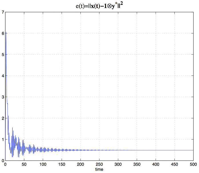
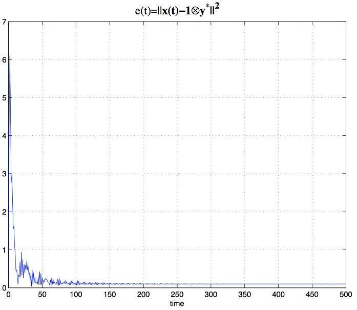
Next, we study the case where all graphs in 𝒬superscript𝒬\mathcal{Q}^{\ast} satisfy the condition of Theorem 1.(ii), i.e., neither of the graphs in the switching graph signal will be able to provide convergent solutions under (4).
Refer to caption
(a) T=0.5
Refer to caption
(b) T=0.25
Refer to caption
(c) T=0.1
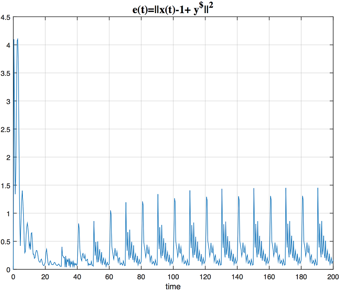
Figure 13: The trajectories of e(t)=𝐱(t)𝟏5𝐲2𝑒𝑡superscriptnorm𝐱𝑡tensor-productsubscript15superscript𝐲2e(t)=\|\mathbf{x}(t)-\mathbf{1}_{5}\otimes\mathbf{y}^{\ast}\|^{2} for i=1,2,3,4,5𝑖12345i=1,2,3,4,5 when (a) T=0.5𝑇0.5T=0.5, (b) T=0.25𝑇0.25T=0.25, (c) T=0.1𝑇0.1T=0.1.

Example 6. Consider a linear equation (1) with respect to 𝐲𝐲\mathbf{y} where

𝐇=[320131211.572320.51],𝐳=[15310].formulae-sequence𝐇matrix320131211.572320.51𝐳matrix15310\mathbf{H}=\begin{bmatrix}3&2&0\\ 1&-3&-1\\ 2&1&1.5\\ -7&-2&3\\ 2&-0.5&1\end{bmatrix},\ \mathbf{z}=\begin{bmatrix}1\\ 5\\ 3\\ -1\\ 0\end{bmatrix}.

It can be easily calculated that the unique least squares solution is 𝐲=[0.751.12 0.53]superscript𝐲superscriptdelimited-[]0.751.120.53top\mathbf{y}^{\ast}=[0.75\ -1.12\ 0.53]^{\top}. At the same time, the condition of Theorem 1.(ii) holds for both 𝒢1subscript𝒢1\mathcal{G}_{1} and 𝒢2subscript𝒢2\mathcal{G}_{2}. Let 𝐱(0)=[10.5 1 0.80.75 0.5 0.70.60.30.81.6 0.25 0.51 0.7]𝐱0superscriptdelimited-[]10.510.80.750.50.70.60.30.81.60.250.510.7top\mathbf{x}(0)=[-1\ -0.5\ 1\ 0.8\ -0.75\ 0.5\ 0.7\ -0.6\ -0.3\ -0.8\ -1.6\ 0.25\ 0.5\ -1\ 0.7]^{\top}, 𝐯(0)=𝟏15𝐯0subscript115\mathbf{v}(0)=\mathbf{1}_{15} be the initial condition. In Figure 13 we plot the trajectories of e(t)=𝐱(t)𝟏5𝐲2𝑒𝑡superscriptnorm𝐱𝑡tensor-productsubscript15superscript𝐲2e(t)=\|\mathbf{x}(t)-\mathbf{1}_{5}\otimes\mathbf{y}^{\ast}\|^{2} for T=0.5,0.25,0.1𝑇0.50.250.1T=0.5,0.25,0.1, respectively. We can see in the three cases that e(t)𝑒𝑡e(t) asymptotically tends to a neighborhood of zero as t𝑡t goes to infinity. Furthermore, the faster the network switches, the smaller such neighborhood becomes. Then the trajectories of (𝐯i(t))[1]subscript𝐯𝑖𝑡delimited-[]1(\mathbf{v}_{i}(t))[1], (𝐯i(t))[2]subscript𝐯𝑖𝑡delimited-[]2(\mathbf{v}_{i}(t))[2], (𝐯i(t))[3]subscript𝐯𝑖𝑡delimited-[]3(\mathbf{v}_{i}(t))[3], i=1,2,3,4,5𝑖12345i=1,2,3,4,5 for T=0.5,0.25,0.1𝑇0.50.250.1T=0.5,0.25,0.1, respectively, are plotted in Figure 14. We find again that 𝐯(t)𝐯𝑡\mathbf{v}(t) tends to fall in a neighborhood of a fixed point as time grows to infinity.

Remarkably enough, neither 𝒢1subscript𝒢1\mathcal{G}_{1} or 𝒢2subscript𝒢2\mathcal{G}_{2} alone will be able to produce trajectories for the 𝐱i(t)subscript𝐱𝑖𝑡\mathbf{x}_{i}(t) that converge even to a neighborhood of the least square solutions, as proved in Theorem 1. The above numerical example clearly reveals the possibility that the two graphs 𝒢1subscript𝒢1\mathcal{G}_{1} and 𝒢2subscript𝒢2\mathcal{G}_{2} can cooperate by a fast switching signal, under which the resulting node dynamics can be driven to a small neighborhood around the least square solution of Eq. (1). It will be interesting to look at the mechanism behind such a surprising phenomenon.
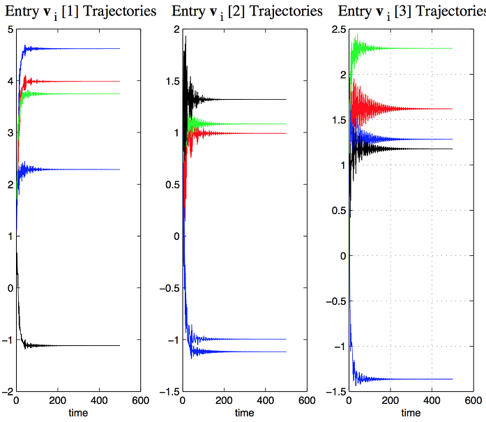
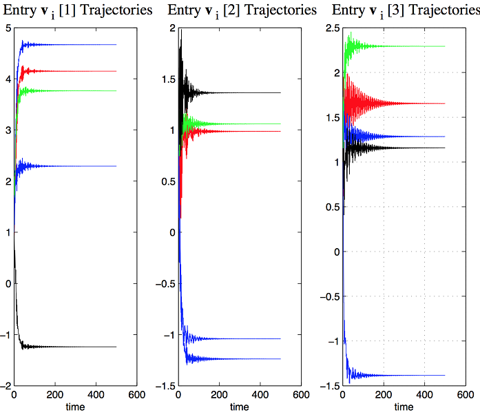
Refer to caption
(a) T=0.5
Refer to caption
(b) T=0.25
Refer to caption
(c) T=0.1
Figure 14: The trajectories of (𝐯i(t))[1]subscript𝐯𝑖𝑡delimited-[]1(\mathbf{v}_{i}(t))[1], (𝐯i(t))[2]subscript𝐯𝑖𝑡delimited-[]2(\mathbf{v}_{i}(t))[2], (𝐯i(t))[3]subscript𝐯𝑖𝑡delimited-[]3(\mathbf{v}_{i}(t))[3] for i=1,2,3,4,5𝑖12345i=1,2,3,4,5 when (a) T=0.5𝑇0.5T=0.5, (b) T=0.25𝑇0.25T=0.25, (c) T=0.1𝑇0.1T=0.1.

6 Conclusions

We studied the problem of obtaining the least squares solution to a linear algebraic equation using distributed algorithms. Each node has the information of one scalar linear equation and holds a dynamic state. Two distributed algorithms in continuous time and discrete time respectively were developed as least squares solvers for linear equations. Under certain conditions, all node states can reach a consensus, which gives the least square solution, by exchanging information with neighbors over a network. To verify the convergence result, some numerical examples were provided. Besides, the feasibility of several fundamental graphs was discussed. Finally, methods of computing residual vectors at individual nodes and alternative state expansion method were discussed, and we also investigated the performance of the proposed flow under switching networks. Remarkably, switching networks at high switching frequencies define an approximate least squares solver even if all graphs in the switching signal fail to do so in the absence of structure switching. Future directions currently being contemplated include establishing the convergence rate of the distributed algorithms, distributed identification of the residual vector, which can be of practical interest and modifying the underlying cost function or adding constraints on it to reflect objectives such as outlier suppression.

References

  • [1] M. J Ablowitz and A. S. Fokas. Complex variables: introduction and applications. Cambridge University Press, 2003.
  • [2] A. Ahmed and E. P. Xing. Recovering time-varying networks of dependencies in social and biological studies. Proceedings of the National Academy of Sciences, 106(29):11878–11883, 2009.
  • [3] B. Anderson, S. Mou, A. S. Morse, and U. Helmke. Decentralized gradient algorithm for solution of a linear equation. Numerical Algebra, Control and Optimization, to appear(preprint arXiv:1509.04538).
  • [4] K. J. Arrow, L. Hurwicz, and H. Uzawa. Studies in linear and non-linear programming. With contributions by H. B. Chenery, S. M. Johnson, S. Karlin, T. Marschak, R. M. Solow. Stanford Mathematical Studies in the Social Sciences, vol. II. Stanford University Press, Stanford, Calif., 1958.
  • [5] R. Ayari, I. Hafnaoui, A. Aguiar, P. Gilbert, M. Galibois, J.-P. Rousseau, G. Beltrame, and G. Nicolescu. Multi-objective mapping of full-mission simulators on heterogeneous distributed multi-processor systems. The Journal of Defense Modeling and Simulation: Applications, Methodology, Technology, page 1548512916657907, 2016.
  • [6] D. P Bertsekas. Nonlinear programming. Athena scientific Belmont, 1999.
  • [7] S. Boyd and L. Vandenberghe. In Convex optimization, pages 215–227. Cambridge university press, 2004.
  • [8] C. A. F. De Rose, H.-U. Heiss, and B. Linnert. Distributed dynamic processor allocation for multicomputers. Parallel Computing, 33(3):145–158, 2007.
  • [9] A. J. Elbirt and C. Paar. An instruction-level distributed processor for symmetric-key cryptography. IEEE Transactions on Parallel and distributed Systems, 16(5):468–480, 2005.
  • [10] P. A. Fuhrmann and U. Helmke. The mathematics of networks of linear systems. Springer, 2015.
  • [11] M. Garland, S. Le Grand, J. Nickolls, J. Anderson, J. Hardwick, Scott Morton, Everett Phillips, Yao Zhang, and Vasily Volkov. Parallel computing experiences with cuda. Micro, IEEE, 28(4):13–27, 2008.
  • [12] B. Gharesifard and J. Cortés. Distributed continuous-time convex optimization on weight-balanced digraphs. IEEE Transactions on Automatic Control, 59(3):781–786, March 2014.
  • [13] B. Gharesifard and J. Cortés. Distributed continuous-time convex optimization on weight-balanced digraphs. IEEE Transactions on Automatic Control, 59(3):781–786, 2014.
  • [14] R. M. Gower and P. Richtárik. Randomized iterative methods for linear systems. SIAM Journal on Matrix Analysis and Applications, 36(4):1660–1690, 2015.
  • [15] D. Jakovetić, J. Xavier, and J. M. ……………..F. Moura. Fast distributed gradient methods. IEEE Transactions on Automatic Control, 59(5):1131–1146, 2014.
  • [16] S. Kaczmarz. Angenäherte auflösung von systemen linearer gleichungen. Bulletin International de l’Academie Polonaise des Sciences et des Lettres, 35:355–357, 1937.
  • [17] S. W. Keckler, W. J. Dally, B. Khailany, M. Garland, and D. Glasco. Gpus and the future of parallel computing. IEEE Micro, 31(5):7–17, 2011.
  • [18] J. Kelner. Lecture 2, 2009 (accessed 11/10/2016). https://ocw.mit.edu/courses/mathematics/.
  • [19] Alan J Laub. In Matrix analysis for scientists and engineers, pages 139–148. Siam, 2005.
  • [20] J. Liu, S. Mou, and A. S. Morse. An asynchronous distributed algorithm for solving a linear algebraic equation. In 52nd IEEE Conference on Decision and Control, pages 5409–5414, 2013.
  • [21] J. Lu and C. Y. Tang. Distributed asynchronous algorithms for solving positive definite linear equations over networks—Part I: Agent networks. IFAC Proceedings Volumes, 42(20):252–257, 2009.
  • [22] J. Lu and C. Y. Tang. Distributed asynchronous algorithms for solving positive definite linear equations over networks—Part II: Wireless networks. IFAC Proceedings Volumes, 42(20):258–263, 2009.
  • [23] A. Margaris, S. Souravlas, and M. Roumeliotis. Parallel implementations of the jacobi linear algebraic systems solve. preprint arXiv:1403.5805, 2014.
  • [24] A.p S. Morse. Supervisory control of families of linear set-point controllers Part I. exact matching. IEEE Transactions on Automatic Control, 41(10):1413–1431, 1996.
  • [25] S. Mou and A. S. Morse. A fixed-neighbor, distributed algorithm for solving a linear algebraic equation. In Proc. European Control Conference, pages 2269–2273, 2013.
  • [26] S. Mou, J. Liu, and A. S. Morse. A distributed algorithm for solving a linear algebraic equation. IEEE Transactions on Automatic Control, 60(11):2863–2878, 2015.
  • [27] A. Nedic and A. Ozdaglar. Distributed subgradient methods for multi-agent optimization. IEEE Transactions on Automatic Control, 54(1):48–61, 2009.
  • [28] A. Nedic, A. Ozdaglar, and P. A. Parrilo. Constrained consensus and optimization in multi-agent networks. IEEE Transactions on Automatic Control, 55(4):922–938, 2010.
  • [29] Mi. J Neely, E.Modiano, and C. E Rohrs. Dynamic power allocation and routing for time-varying wireless networks. IEEE Journal on Selected Areas in Communications, 23(1):89–103, 2005.
  • [30] A. M. Partl, A. Maselli, B. Ciardi, A. Ferrara, and V. Müller. Enabling parallel computing in crash. Monthly Notices of the Royal Astronomical Society, 414(1):428–444, 2011.
  • [31] M. Pease, R. Shostak, and L. Lamport. Reaching agreement in the presence of faults. Journal of the ACM (JACM), 27(2):228–234, 1980.
  • [32] F. P. Preparata and J. Vuillemin. The cube-connected cycles: a versatile network for parallel computation. Communications of the ACM, 24(5):300–309, 1981.
  • [33] G. Shi, B. Anderson, and U. Helmke. Network flows that solve linear equations. IEEE Transactions on Automatic Control, in press, 2017.
  • [34] J. N. Tsitsiklis, D. P. Bertsekas, and M. Athans. Distributed asynchronous deterministic and stochastic gradient optimization algorithms. In 1984 American Control Conference, pages 484–489, 1984.
  • [35] J. Wang and N. Elia. Control approach to distributed optimization. In Communication, Control, and Computing (Allerton), 2010 48th Annual Allerton Conference on, pages 557–561, Sept 2010.
  • [36] J. Wang and N. Elia. A control perspective for centralized and distributed convex optimization. In 2011 50th IEEE Conference on Decision and Control and European Control Conference, pages 3800–3805, Dec 2011.
  • [37] X. Yang and R. Mittal. Acceleration of the jacobi iterative method by factors exceeding 100 using scheduled relaxation. Journal of Computational Physics, 274:695–708, 2014.
  • [38] D. Young. Iterative methods for solving partial difference equations of elliptic type. Transactions of the American Mathematical Society, 76(1):92–111, 1954.