A Black–Scholes inequality: applications and generalisations

Abstract.

The space of call price functions has a natural noncommutative semigroup structure with an involution. A basic example is the Black–Scholes call price surface, from which an interesting inequality for Black–Scholes implied volatility is derived. The binary operation is compatible with the convex order, and therefore a one-parameter sub-semigroup gives rise to an arbitrage-free market model. It is shown that each such one-parameter semigroup corresponds to a unique log-concave probability density, providing a family of tractable call price surface parametrisations in the spirit of the Gatheral–Jacquier SVI surface. An explicit example is given to illustrate the idea. The key observation is an isomorphism linking an initial call price curve to the lift zonoid of the terminal price of the underlying asset.

1. Introduction

We define the Black–Scholes call price function $C_{\mathrm{BS}}:[0,\infty)\times[0,\infty)\to[0,1]$ by the formula

$$C_{\mathrm{BS}}(\kappa,y) =\int_{-\infty}^{\infty}(\varphi(z+y)-\kappa\ \varphi(z))^{+}dz$$

$$=\left\{\begin{array}[]{ll}{\Phi}\big{(}-\frac{\log\kappa}{y}+\frac{y}{2}\big{)}-\kappa{\Phi}\big{(}-\frac{\log\kappa}{y}-\frac{y}{2}\big{)}&\mbox{ if }y>0,\kappa>0,\\ (1-\kappa)^{+}&\mbox{ if }y=0,\\ 1&\mbox{ if }\kappa=0,\end{array}\right.$$

where $\varphi(z)=\frac{1}{\sqrt{2\pi}}e^{-z^{2}/2}$ is the standard normal density and $\Phi(x)=\int_{-\infty}^{x}\varphi(z)dz$ is its distribution function. Recall the financial context of this definition: a market with a risk-free zero-coupon bond of unit face value, maturity $T$ and initial price $B_{0,T}$; a stock with initial price $S_{0}$ that pays no dividend; and a European call option written on the stock with maturity $T$ and strike price $K$. In the Black–Scholes model, the initial price $C_{0,T,K}$ of the call option is given by the formula

$$C_{0,T,K}=S_{0}\ C_{\mathrm{BS}}\left(\frac{KB_{0,T}}{S_{0}},\sigma\sqrt{T}\right),$$

where $\sigma$ is the volatility of the stock price. In particular, the first argument of $C_{\mathrm{BS}}$ plays the role of the moneyness $\kappa=KB_{0,T}/S_{0}$ and the second argument plays the role of the total standard deviation $y=\sigma\sqrt{T}$ of the terminal log stock price.

The starting point of this note is the following observation.

Theorem 1.0.1.

For $\kappa_{1},\kappa_{2}>0$ and $y_{1},y_{2}>0$ we have

$$C_{\mathrm{BS}}(\kappa_{1}\kappa_{2},y_{1}+y_{2})\leq C_{\mathrm{BS}}(\kappa_{1},y_{1})+\kappa_{1}C_{\mathrm{BS}}(\kappa_{2},y_{2})$$

with equality if and only if

$$-\frac{\log\kappa_{1}}{y_{1}}-\frac{y_{1}}{2}=-\frac{\log\kappa_{2}}{y_{2}}+\frac{y_{2}}{2}.$$

While it is fairly straight-forward to prove Theorem 1.0.1 directly, the proof is omitted as it is a special case of Theorem 3.2.4 below. Indeed, the purpose of this note is to try to understand the fundamental principle that gives rise to such an inequality. As a hint of things to come, it is worth pointing out that the expression $y_{1}+y_{2}$ appearing on the left-hand side of the inequality corresponds to the sum of the standard deviations – not the sum of the variances. From this observation, it may not be surprising to see that a key idea underpinning Theorem 1.0.1 is that of adding comonotonic – not independent – normal random variables. These vague comments will be made precise in Theorem 2.3.3 below.

Before proceeding, we re-express Theorem 1.0.1 in terms of the Black–Scholes implied total standard deviation function, defined for $\kappa>0$ to be the inverse function

$$Y_{\mathrm{BS}}(\kappa,\cdot):[(1-\kappa)^{+},1]\to[0,\infty]$$

such that

$$y=Y_{\mathrm{BS}}(\kappa,c)\Leftrightarrow C_{\mathrm{BS}}(\kappa,y)=c.$$

In particular, the quantity $Y_{\mathrm{BS}}(\kappa,c)$ denotes the implied total standard deviation of an option of moneyness $\kappa$ whose normalised price is $c$. We will find it notationally convenient to set $Y_{\mathrm{BS}}(\kappa,c)=\infty$ for $c\geq 1$. With this notation, we have the following interesting reformulation which requires no proof:

Corollary 1.0.2.

For all $\kappa_{1},\kappa_{2}>0$ and $(1-\kappa_{i})^{+}<c_{i}<1$ for $i=1,2$, we have

$$Y_{\mathrm{BS}}(\kappa_{1},c_{1})+Y_{\mathrm{BS}}(\kappa_{2},c_{2})\leq Y_{\mathrm{BS}}(\kappa_{1}\kappa_{2},c_{1}+\kappa_{1}c_{2})$$

with equality if and only if

$$-\frac{\log\kappa_{1}}{y_{1}}-\frac{y_{1}}{2}=-\frac{\log\kappa_{2}}{y_{2}}+\frac{y_{2}}{2}.$$

where $y_{i}=Y_{\mathrm{BS}}(\kappa_{i},c_{i})$ for $i=1,2$.

To add some context, we recall the following related bounds on the function $C_{\mathrm{BS}}$ and $Y_{\mathrm{BS}}$; see [31, Theorem 3.1].

Theorem 1.0.3.

For all $\kappa>0$, $y>0$, and $0<p<1$ we have

$$C_{\mathrm{BS}}(\kappa,y)\geq\Phi(\Phi^{-1}(p)+y)-p\kappa$$

with equality if and only if

$$p=\Phi\left(-\frac{\log\kappa}{y}-\frac{y}{2}\right).$$

Equivalently, for all $\kappa>0$, $(1-\kappa)^{+}<c<1$ and $0<p<1$ we have

$$Y_{\mathrm{BS}}(\kappa,c)\leq\Phi^{-1}(c+p\kappa)-\Phi^{-1}(p)$$

where $\Phi^{-1}(u)=+\infty$ for $u\geq 1$.

In [31], Theorem 1.0.3 was used to derive upper bounds on the implied total standard deviation function $Y_{\mathrm{BS}}$ by selecting various values of $p$ to insert into the inequality.

The function $\Phi\big{(}\Phi^{-1}(\cdot)+y\big{)}$ has appeared elsewhere in various contexts. For instance, it is the value function for a problem of maximising the probability of hitting a target considered by Kulldorff [27, Theorem 6]. (Also see the book of Karatzas[23, Section 2.6].) In insurance mathematics, the function is often called the Wang transform and was proposed in [33] as a method of distorting a probability distribution in order to introduce a risk premium. In a somewhat unrelated context, Kulik & Tymoshkevych [26] observed, while proving a certain log-Sobolev inequality, that the family of functions $\left(\Phi(\Phi^{-1}(\cdot)+y)\right)_{y\geq 0}$ forms a semigroup under function composition. We will see that this semigroup property is the essential idea of our proof of Theorem 1.0.1 and its subsequent generalisations.

The rest of this note is arranged as follows. In section 2 we introduce a space of call price curves and explore some of its properties. In particular, we will see that it has a natural noncommutative semigroup structure with an involution. The binary operation has a natural financial interpretation as the maximum price of an option to swap the one asset for a fixed number of shares of a second asset. In section 3, we introduce a space of call price surfaces and provide in Theorem 3.1.2 equivalent characterisations in terms of either one supermartingale or two martingales. Furthermore, it is shown that the binary operation is compatible with the decreasing convex order, and therefore a one-parameter semigroup of the space of call curves can be associated with an arbitrage-free market model. A main result of this article is Theorem 3.2.7: each one-parameter semigroup corresponds to a unique (up to translation and scaling) log-concave probability density, generalising the Black–Scholes call price surface and providing a family of reasonably tractable call surface parametrisations in the spirit of the SVI surface. In section 4, further properties of these call price surfaces, including the asymptotics of their implied volatility, are explored. In addition, an explicit example is given to illustrate the idea, and is calibrated to real world call price data. In section 5, the proof of Theorem 3.2.7 is given. The key observation is that the Legendre transform is an isomorphism converting the binary operation on call price curves to function composition. The isomorphism has the additional interpretation as the lift zonoid of the terminal price of the underlying asset.

2. The algebraic properties of call prices

2.1. The space of call price curves

For motivation, consider a market with two (non-dividend paying) assets whose prices at time $t$ are $A_{t}$ and $B_{t}$. We assume that both prices are always non-negative and that the initial prices $A_{0}$ and $B_{0}$ are strictly positive. We further assume that there exists a martingale deflator $Y=(Y_{t})_{t\geq 0}$, that is, a positive adapted process such that the processes $YA$ and $YB$ are both martingales. The assumption of the existence of a martingale deflator ensures that there is no arbitrage in the market. (Conversely, in discrete time, no arbitrage implies the existence a martingale deflator, even if the market does not admit a numéraire portfolio; see [32].)

Now introduce an option to swap one share of asset $A$ with $K$ shares of asset $B$ at a fixed time $T>0$, so the payout is $(A_{T}-KB_{T})^{+}$. If the asset $B$ is a risk-free zero-coupon bond of maturity $T$ and unit face value, then the option is a standard call option. It will prove useful in our discussion to let asset $B$ be arbitrary, but we shall still refer to this option as a call option.

There is no arbitrage in the augmented market if the time $t$ price of this call option is

$$C_{t,T,K}=\frac{1}{Y_{t}}\mathbb{E}[Y_{T}(A_{T}-KB_{T})^{+}|\mathcal{F}_{t}].$$

In particular, setting

$$\alpha=\frac{Y_{T}A_{T}}{Y_{0}A_{0}}\ \mbox{ and }\ \beta=\frac{Y_{T}B_{T}}{Y_{0}B_{0}}$$

the initial price of this option, normalised by the initial price of asset $A$ can be written as

$$\frac{C_{0,T,K}}{A_{0}}=\mathbb{E}[(\alpha-\kappa\beta)^{+}].$$

where the moneyness is given by

$$\kappa=\frac{KB_{0}}{A_{0}}.$$

The above discussion motivates the following definition:

Definition 2.1.1.

A function $C:[0,\infty)\to[0,1]$ is a call price curve iff there exist non-negative random variables $\alpha$ and $\beta$ defined on some probability space such that

$$\mathbb{E}(\alpha)=1=\mathbb{E}(\beta).$$

and

$$C(\kappa)=\mathbb{E}[(\alpha-\kappa\beta)^{+}]\mbox{ for all }\kappa\geq 0,$$

in which case the ordered pair $(\alpha,\beta)$ of random variables is called a basic representation of $C$. The set of all call price curves is denoted $\mathcal{C}$.

From a practical perspective, the normalised call price $C(\kappa)$ is directly observed, while the law of the pair $(\alpha,\beta)$ is not. Therefore, a theme of this note is to try to express notions in terms of the call price curve. Here is a first result of this type.

Theorem 2.1.2.

Given a function $C:[0,\infty)\to[0,1]$, the following are equivalent:

1. $C\in\mathcal{C}$.

2. There exists a non-negative random variable $S$ with $\mathbb{E}(S)\leq 1$ such that

   $$C(\kappa)=1-\mathbb{E}[S\wedge\kappa]\mbox{ for all }\kappa\geq 0.$$

3. $C$ is convex and such that $C(\kappa)\geq(1-\kappa)^{+}$ for all $\kappa\geq 0$.

Furthermore, in case (2) we have that

$$\mathbb{P}(S>0)=-C^{\prime}(0)\mbox{ and }\mathbb{E}(S)=1-C(\infty).$$

and more generally that

$$\mathbb{P}(S>\kappa)=-C^{\prime}(\kappa)\mbox{ for all }\kappa\geq 0,$$

where $C^{\prime}$ denotes the right-derivative of $C$.

Proof.

The implications (1)$\Rightarrow$(3) and (2)$\Rightarrow$(3) are straightforward, so their proofs are omitted. Furthermore, the claim that the distribution of $S$ can be recovered from $C$ is essentially the Breeden & Litzenberger [3] formula.

(3)$\Rightarrow$(2): By convexity, the right-derivative $C^{\prime}$ is defined everywhere and is non-decreasing and right-continuous. Furthermore, since $(1-\kappa)^{+}\leq C(\kappa)\leq 1$ for all $\kappa$ we have $-1\leq C^{\prime}(\kappa)\leq 0$ for all $\kappa$. Let $S$ be a random variable such that $\mathbb{P}(S>\kappa)=-C^{\prime}(\kappa)$. Note that

$$\mathbb{E}[S\wedge\kappa] =\mathbb{E}\int_{0}^{\kappa}\mathbbm{1}_{\{u<S\}}du$$

$$=\int_{0}^{\kappa}\mathbb{P}(S>u)du$$

$$=1-C(\kappa)$$

by Fubini’s theorem and the absolute continuity of the convex function $C$.

It remains to show that either (2)$\Rightarrow$(1) or (3)$\Rightarrow$(1). That is, we must construct a basic representation $(\alpha,\beta)$ from either the random variable $S$ or the function $C$. We will give a construction showing (2)$\Rightarrow$(1) in the proof of Theorem 2.3.2, and a rather different construction showing (3)$\Rightarrow$(1) in the proof of Theorem 3.1.2. To avoid repetition, we omit a construction here. ∎

By definition, a call price curve $C$ is determined by two random variables $\alpha$ and $\beta$. However, the distribution of the pair $(\alpha,\beta)$ cannot be inferred solely from $C$. In contrast, Theorem 2.1.2 above says that a call price curve $C$ is also determined by a single random variable $S$, and furthermore, the law of $S$ is unique and can be recovered from $C$. This observation motivates the following definition.

Definition 2.1.3.

Given a call price curve $C\in\mathcal{C}$, suppose that $S$ is a non-negative random variable such that $C(\kappa)=1-\mathbb{E}[S\wedge\kappa]$ for all $\kappa\geq 0$. Then $S$ is called a primal representation of $C$.

Remark 2.1.4.

As hinted by the name primal, we will shortly introduce a dual representation.

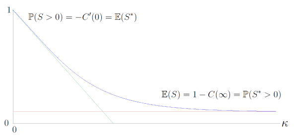
Figure 1 plots the graph of a typical element $C\in\mathcal{C}$.

Figure 1. The graph of a typical function $C\in\mathcal{C}$

Remark 2.1.5.

An example of an element of $\mathcal{C}$ is the Black–Scholes call price function $C_{\mathrm{BS}}(\cdot,y)$ for any $y\geq 0$. A primal representation is

$$S^{(y)}=\frac{\varphi(Z+y)}{\varphi(Z)}=e^{-yZ-y^{2}/2}$$

where $Z\sim N(0,1)$ has the standard normal distribution.

Remark 2.1.6.

We note that there are alternative financial interpretations of call price curves $C\in\mathcal{C}$ in the case $C(\infty)>0$. One popularised by Cox & Hobson [10] is to model the primal representation as the terminal price $S$ of an asset experiencing a bubble in the sense that the price process discounted by the price of the risk-free $T$-zero coupon bond is a strictly local martingale under a fixed $T$-forward measure. For this interpretation, the option payout must be modified: rather than the payout of standard (naked) call option, in this interpretation the quantity $C(\kappa)$ models the normalised price of a fully collateralised (covered) call with payout

$$(S-\kappa)^{+}+1-S=1-S\wedge\kappa.$$

In my view, there are two related shortcomings of this interpretation. Firstly, this type of bubble phenomenon can only arise in continuous time models, since in discrete time non-negative local martingales are necessarily true martingales. Secondly, in the case $\mathbb{E}(S)<1$ where the underlying stock is not priced by expectation, it is not clear from a modelling perspective why the market should then price the call option by expectation $C(\kappa)=\mathbb{E}[(S-\kappa)^{+}+1-S].$ Both shortcomings highlight the subtlety of continuous time arbitrage theory, in particular, the sensitive dependence on the choice of numéraire on the definition of arbitrage (and related arbitrage-like conditions).

2.2. The involution

There is a natural involution on the space of call prices:

Definition 2.2.1.

Given a call price curve $C\in\mathcal{C}$ with basic representation $(\alpha,\beta)$, the function $C^{*}$ is the call price curve with basic representation $(\beta,\alpha)$.

This leads to a straightforward financial interpretation of the involution. As described above, we may think of $C(\kappa)$ as the initial price, normalised by $A_{0}$, of the option to swap one share of asset $A$ for $K$ shares of asset $B$, where $KB_{0}=\kappa A_{0}$. Then $C^{*}(\kappa)$ is the initial price, normalised by $B_{0}$, of the option to swap one share of asset $B$ for $K^{*}$ shares of asset $A$, where $K^{*}A_{0}=\kappa B_{0}$.

We now record a fact about this involution ^∗, expressed directly in terms of call prices. The proof is a straightforward verification, and hence omitted.

Theorem 2.2.2.

Fix $C\in\mathcal{C}$. Then $C^{*}(0)=1$ and

$$C^{*}(\kappa)=1-\kappa+\kappa C(1/\kappa)\mbox{ for all }\kappa>0.$$

Remark 2.2.3.

As an example, notice for the Black–Scholes call function we have

$$C_{\mathrm{BS}}(\cdot,y)^{*}=C_{\mathrm{BS}}(\cdot,y)\mbox{ for all }y\geq 0$$

by the classical put-call symmetry formula.

Remark 2.2.4.

The function $C^{*}$ is related to the well-known perspective function of the convex function $C$ defined by $(\eta,\kappa)\mapsto\eta\ C(\kappa/\eta)$; see, for instance, the book of Boyd & Vanderberghe [6, Section 3.2.6].

As hinted at above, we can define another random variable in terms of this involution:

Definition 2.2.5.

Given a call price curve $C\in\mathcal{C}$, a non-negative random variable $S^{*}$ is a dual representation of $C$ iff $S^{*}$ is a primal representation of the call price curve $C^{*}$.

That this dual random variable should be called a representation of a call price is due to the following observation. Again the proof is straightforward and hence omitted.

Theorem 2.2.6.

Given a call price $C\in\mathcal{C}$ with dual representation $S^{*}$ we have

$$C(\kappa)=\mathbb{E}[(1-S^{*}\kappa)^{+}]=1-\mathbb{E}[1\wedge(S^{*}\kappa)]\mbox{ for all }\kappa\geq 0.$$

In particular, we have

$$\mathbb{P}(S^{*}>0)=1-C(\infty)\mbox{ and }\mathbb{E}(S^{*})=-C^{\prime}(0).$$

Finally, for all $\kappa\geq 0$ we have

$$C(\kappa) =\mathbb{P}(S^{*}<1/\kappa)-\kappa\mathbb{P}(S>\kappa)$$

$$=\mathbb{P}(S^{*}\leq 1/\kappa)-\kappa\mathbb{P}(S\geq\kappa).$$

Remark 2.2.7.

See the papers of De Marco, Hillairet & Jacquier [11] and Jacquier & Keller-Ressel [21] for a related financial interpretation of the relationship between the primal and dual representations in terms of a continuous time market possibly experiencing a bubble à la Cox & Hobson.

2.3. The binary operation

We have introduced one algebraic operation, the involution ^∗, to the set of call price curves. We now come to the second algebraic operation which will help to contextualise the Black–Scholes inequality of Theorem 1.0.1. To motivate it, consider a market with three assets with time $t$ prices $A_{1,t},A_{2,t}$ and $B_{t}$. We know the initial cost of an option to swap one share of asset $A_{1}$ with $H_{1}$ shares of asset $B$, as well as the initial cost of an option to swap one share of asset $B$ with $H_{2}$ shares of asset $A_{2}$, for various values of $H_{1}$ and $H_{2}$, where all of the options mature at a fixed date $T>0$. Our goal is the find an upper bound on the cost of an option to swap one share of asset $A_{1}$ for $K$ shares of asset $A_{2}$, for the same maturity date $T$.

Definition 2.3.1.

For call price curves $C_{1},C_{2}\in\mathcal{C}$, define a binary operation $\bullet$ on $\mathcal{C}$ by

$$C_{1}\bullet C_{2}(\kappa)=\sup_{\alpha_{1},\beta,\alpha_{2}}\mathbb{E}[(\alpha_{1}-\kappa\alpha_{2})^{+}]$$

where the supremum is taken over non-negative random variables $\alpha_{1},\beta,\alpha_{2}$ defined on the same probability space such that $(\alpha_{1},\beta)$ is a basic representation of $C_{1}$ and $(\beta,\alpha_{2})$ is a basic representation of $C_{2}$.

At this stage, it is not immediately clear that given two call price curves $C_{1}$ and $C_{2}$ one can find a triple $(\alpha_{1},\beta,\alpha_{2})$ satisfying the definition of the binary operation $\bullet$, and in principle, we should complete the definition with the usual convention that $\sup\emptyset=-\infty$. Fortunately, this caveat is not necessary as can be deduced from the following result:

Theorem 2.3.2.

For call price curves $C_{1},C_{2}\in\mathcal{C}$ we have

$$C_{1}\bullet C_{2}(\kappa)=\sup_{S_{1},S_{2}^{*}}\left\{1-\mathbb{E}[S_{1}\wedge(S_{2}^{*}\kappa)]\right\},$$

where the supremum is taken over random variables $S_{1}$ and $S_{2}^{*}$ defined on the same space, where $S_{1}$ is a primal representation of $C_{1}$ and $S_{2}^{*}$ is a dual representation of $C_{2}$.

Proof.

First, let $S_{1}$ be a primal representation of $C_{1}$ and $S_{2}^{*}$ be a dual representation of $C_{2}$, defined on the same probability space. We will exhibit random variables $(\alpha_{1},\beta,\alpha_{2})$ such that $(\alpha_{1},\beta)$ is a basic representation of $C_{1}$ and $(\beta,\alpha_{2})$ is a basic representation of $C_{2}$.

For the construction, we introduce Bernoulli random variables $\gamma_{1},\gamma_{2},\delta_{1},\delta_{2}$, independent of $(S_{1},S_{2}^{*})$ and each other, with

$$\mathbb{P}(\gamma_{1}=1)=\mathbb{E}(S_{1}),\ \mathbb{P}(\gamma_{2}=1)=\mathbb{E}(S_{2}^{*})\mbox{ and }\mathbb{P}(\delta_{1}=1)=\mathbb{P}(\delta_{2}=1)=\tfrac{1}{2}.$$

If $\mathbb{P}(S_{1}=0)<1$ then set

$$a_{1}=\frac{S_{1}}{\mathbb{E}(S_{1})}\mbox{ and }b_{1}=\frac{\gamma_{1}}{\mathbb{E}(S_{1})}$$

and if $S_{1}=0$ almost surely, set $a_{1}=2\delta_{1}$ and $b_{1}=2(1-\delta_{1})$. Similarly, if $\mathbb{P}(S_{2}^{*}=0)<1$ then set

$$a_{2}=\frac{S_{2}^{*}}{\mathbb{E}(S_{2}^{*})}\mbox{ and }b_{2}=\frac{\gamma_{2}}{\mathbb{E}(S_{2}^{*})}$$

and if $S_{2}^{*}=0$ almost surely, set $a_{2}=2\delta_{2}$ and $b_{2}=2(1-\delta_{2})$. Finally set

$$\alpha_{1}=a_{1}b_{2},\ \ \beta=b_{1}b_{2},\ \ \alpha_{2}=a_{2}b_{1}.$$

It is easy to check that the triplet $(\alpha_{1},\beta,\alpha_{2})$ is the desired representation. This shows

$$C_{1}\bullet C_{2}(\kappa)\geq\sup_{S_{1},S_{2}^{*}}\left\{1-\mathbb{E}[S_{1}\wedge(S_{2}^{*}\kappa)]\right\},$$

For the reverse inequality, given a basic representation $(\alpha_{1},\beta)$ of $C_{1}$ and a basic representation $(\beta,\alpha_{2})$ of $C_{2}$ defined on the same probability space $(\Omega,\mathcal{F},\mathbb{P})$, we let

$$S_{1}=\frac{\alpha_{1}}{\beta}\mathbbm{1}_{\{\beta>0\}}\mbox{ and }S_{2}^{*}=\frac{\alpha_{2}}{\beta}\mathbbm{1}_{\{\beta>0\}}$$

and an absolutely continuous measure $\mathbb{P}^{\beta}$ by $\frac{d\mathbb{P}^{\beta}}{d\mathbb{P}}=\beta.$ It is easy to check that $S_{1}$ is a primal representation of $C_{1}$ and $S_{2}^{*}$ is a dual representation of $C_{2}$ under $\mathbb{P}^{\beta}$ and that

$$\mathbb{E}[(\alpha_{1}-\kappa\alpha_{2})^{+}] \leq 1-\mathbb{E}[\alpha_{1}\wedge(\alpha_{2}\kappa)\mathbbm{1}_{\{\beta>0\}}]$$

$$=1-\mathbb{E}^{\beta}[S_{1}\wedge(S_{2}^{*}\kappa)].$$

∎

Given the laws of two random variables $X_{1}$ and $X_{2}$ and a convex function $g$, it is well-known that the quantity

$$\mathbb{E}[g(X_{1}+X_{2})]$$

is maximised when $X_{1}$ and $X_{2}$ are comonotonic. See, for instance, the paper of Kaas–Dhaene–Vyncke–Goovaerts– Denuit [22] for a proof. By rewriting the expression

$$1-S_{1}\wedge(S_{2}^{*}\kappa)=(S_{1}-\kappa S_{2}^{*})^{+}+1-S_{1}$$

we see that the supremum defining the binary operation $\bullet$ is achieved when $S_{1}$ and $S^{*}_{2}$ are countermonotonic. We will recover this fact in the following result, which also continues our theme of expressing notions directly in terms of the call prices. In this case, the binary operation $\bullet$ can be expressed via a minimisation problem:

Theorem 2.3.3.

Let $S_{1}$ be a primal representation of $C_{1}\in\mathcal{C}$, and $S_{2}^{*}$ a dual representation of $C_{2}\in\mathcal{C}$, where $S_{1}$ and $S_{2}^{*}$ are defined on the same probability space. Then

$$1-\mathbb{E}[S_{1}\wedge(\kappa S_{2}^{*})]\leq C_{1}(\eta)+\eta\ C_{2}(\kappa/\eta)$$

for all $\kappa\geq 0$ and $\eta\geq 0$, with convention $0\ C_{2}(\kappa/0)=0$. There is equality if the following hold true:

1. $S_{1}$ and $S_{2}^{*}$ are countermonotonic, and

2. $\mathbb{P}(S_{1}<\eta)\leq\mathbb{P}(S_{2}^{*}\geq\eta/\kappa)$ and $\mathbb{P}(S_{1}\leq\eta)\geq\mathbb{P}(S_{2}^{*}>\eta/\kappa).$

In particular, we have

$$C_{1}\bullet C_{2}(\kappa)=\inf_{\eta\geq 0}[C_{1}(\eta)+\eta C_{2}(\kappa/\eta)]\mbox{ for all }\kappa\geq 0.$$

Proof.

Recall that for real $a,b$ we have

$$(a+b)^{+}\leq a^{+}+b^{+}$$

with equality if $ab\geq 0$. Hence, fixing $\kappa\geq 0$, we have

$$1-\mathbb{E}[S_{1}\wedge(S_{2}^{*}\kappa)] =\mathbb{E}[(S_{1}-\kappa S^{*}_{2})^{+}]+1-\mathbb{E}(S_{1})$$

$$\leq\mathbb{E}[(S_{1}-\eta)^{+}]+1-\mathbb{E}(S_{1})+\mathbb{E}[(\eta-\kappa S^{*}_{2})^{+}]$$

$$=C_{1}(\eta)+\eta C_{2}(\kappa/\eta).$$

for all $\eta\geq 0$.

Now pick $\eta\geq 0$ such that

$$\mathbb{P}(S_{1}<\eta)\leq\mathbb{P}(S_{2}^{*}\geq\eta/\kappa)$$

and

$$\mathbb{P}(S_{1}\leq\eta)\geq\mathbb{P}(S_{2}^{*}>\eta/\kappa).$$

Also assume that $S_{1}$ and $S_{2}^{*}$ are countermonotonic so that

$$\{S_{1}<\eta\}\subseteq\{S_{2}^{*}\geq\eta/\kappa\}$$

and

$$\{S_{1}\leq\eta\}\supseteq\{S_{2}^{*}>\eta/\kappa\}.$$

Notice that in this case, we have

$$(S_{1}-\eta)(\eta-\kappa S^{*}_{2})\geq 0\mbox{ almost surely}$$

and hence there is equality in the inequality above. ∎

Remark 2.3.4.

This result is related to the upper bound on basket options found by Hobson, Laurence & Wang [20, Theorem 3.1].

Remark 2.3.5.

Given the conclusion of Theorem 2.3.3 we caution that the operation $\bullet$ is not the well-known inf-convolution $\square$; however, we will see in section 5.2 below that $\bullet$ is related to the inf-convolution $\square$ via an exponential map.

In light of the formula for the binary operation $\bullet$ appearing in Theorem 2.3.3, the Black–Scholes inequality of Theorem 1.0.1 amounts to the claim that for $y_{1},y_{2}\geq 0$ we have

$$C_{\mathrm{BS}}(\cdot,y_{1})\bullet C_{\mathrm{BS}}(\cdot,y_{2})=C_{\mathrm{BS}}(\cdot,y_{1}+y_{2}).$$

This is a special case of Theorem 3.2.4, stated and proven below.

We now come to the key observation of this note. To state it, we distinguish two particular elements $E,Z\in\mathcal{C}$ defined by

$$E(\kappa)=(1-\kappa)^{+}\mbox{ and }Z(\kappa)=1\mbox{ for all }\kappa\geq 0.$$

Note that the random variables representing $E$ and $Z$ are constant, with $S=1=S^{*}$ representing $E$ and $S=0=S^{*}$ representing $Z$. The following result shows that $\mathcal{C}$ is a noncommutative semigroup with respect to $\bullet$ with involution ^∗, where $E$ is the identity element $Z$ is the absorbing element. The proof is straightforward, and hence omitted.

Theorem 2.3.6.

For every $C,C_{1},C_{2},C_{3}\in\mathcal{C}$ we have

1. $C_{1}\bullet C_{2}\in\mathcal{C}.$

2. $C_{1}\bullet(C_{2}\bullet C_{3})=(C_{1}\bullet C_{2})\bullet C_{3}.$

3. $(C_{1}\bullet C_{2})^{*}=C_{2}^{*}\bullet C_{1}^{*}$.

4. $E\bullet C=C\bullet E=C.$

5. $Z\bullet C=C\bullet Z=Z.$

We conclude this section by introducing two useful subsets of the set of call price curves.

Definition 2.3.7.

Let

$$\mathcal{C}_{+}=\{C\in\mathcal{C}:C^{\prime}(0)=-1\}.$$

and

$$\mathcal{C}_{1}=\{C\in\mathcal{C}:C(\infty)=0\}.$$

That is, fix a call price curve $C\in\mathcal{C}$ with primal representation $S$ and dual representation $S^{*}$. The call price curve $C$ is in $\mathcal{C}_{+}$ if and only if $\mathbb{P}(S>0)=\mathbb{E}(S^{*})=1$, while $C$ is in $\mathcal{C}_{1}$ if and only if $\mathbb{P}(S^{*}>0)=\mathbb{E}(S)=1$.

Remark 2.3.8.

As an example, notice that for the Black–Scholes call function we have

$$C_{\mathrm{BS}}(\cdot,y)\in C_{1}\cap C_{+}\mbox{ for all }y\geq 0.$$

The subsets $\mathcal{C}_{+}$ and $\mathcal{C}_{1}$ are closed with respect to the binary operation.

Proposition 2.3.9.

Given $C_{1},C_{2}\in\mathcal{C}$ we have

1. $C_{1}\bullet C_{2}\in\mathcal{C}_{1}$ if and only if both $C_{1}\in\mathcal{C}_{1}$ and $C_{2}\in\mathcal{C}_{1}$.

2. $C_{1}\bullet C_{2}\in\mathcal{C}_{+}$ if and only if both $C_{1}\in\mathcal{C}_{+}$ and $C_{2}\in\mathcal{C}_{+}$.

Proof.

By Theorem 2.3.3 we have

$$C_{1}\bullet C_{2}(\kappa)=1-\mathbb{E}[S_{1}\wedge(\kappa S_{2}^{*})]\mbox{ for all }\kappa\geq 0$$

where $S_{1}$ is a primal representation of $C_{1}$, where $S_{2}^{*}$ is a dual representation of $C_{2}$ and $S_{1}$ and $S_{2}^{*}$ are countermonotonic. For implication (1) note that

$$\mathbb{E}[S_{1}\wedge(\kappa S_{2}^{*})]\to 1\mbox{ as }\kappa\to\infty$$

if and only if

$$\mathbb{E}(S_{1})=1\mbox{ and }\mathbb{P}(S_{2}^{*}>0)=1.$$

For implication (2), apply Theorem 2.3.6 (3) and the fact that $(\mathcal{C}_{+})^{*}=\mathcal{C}_{1}$. ∎

3. One-parameter semigroups, peacocks and lyrebirds

3.1. The space of call price surfaces

With the motivation at the beginning of section 2 we consider the family of prices of options when the maturity date is allowed to vary. We now introduce the following definition:

Definition 3.1.1.

A call price surface is a function $C:[0,\infty)\times[0,\infty)\to[0,1]$ such that there exists an pair of non-negative martingales $(\alpha_{t},\beta_{t})_{t\geq 0}$ such that

$$\alpha_{0}=1=\beta_{0}$$

and

$$C(\kappa,t)=\mathbb{E}[(\alpha_{t}-\kappa\beta_{t})^{+}]\mbox{ for all }\kappa\geq 0,t\geq 0.$$

Our goal is to understand the structure the space of call price surfaces, and relate this structure to the binary operation $\bullet$ introduced in the last section.

Theorem 3.1.2.

Given a function $C:[0,\infty)\times[0,\infty)\to[0,1]$ the following are equivalent:

1. $C$ is a call price surface

2. There exists a non-negative supermartingale $S$ such that $S_{0}=1$ and

   $$C(\kappa,t)=1-\mathbb{E}[S_{t}\wedge\kappa]\mbox{ for all }(\kappa,t).$$

3. There exists a non-negative supermartingale $S^{*}$ such that $S^{*}_{0}=1$ and

   $$C(\kappa,t)=1-\mathbb{E}[1\wedge(\kappa S^{*}_{t})]\mbox{ for all }(\kappa,t).$$

4. For all $\varepsilon>0$, there exist bounded non-negative martingales $\alpha$ and $\beta$ such that $\alpha_{0}=1=\beta_{0}$ and

   $$C(\kappa,t)=\mathbb{E}[(\alpha_{t}-\kappa\beta_{t})^{+}]\mbox{ for all }(\kappa,t)$$

   and such that $\alpha_{t}+\varepsilon\beta_{t}=1+\varepsilon$ for all $t\geq 0$.

5. $C(\kappa,\cdot)$ is non-decreasing with $C(\kappa,0)=(1-\kappa)^{+}$ for all $\kappa\geq 0$, and $C(\cdot,t)$ is convex for all $t\geq 0$.

Proof.

The implications ($n$) $\Rightarrow$ (5) for $1\leq n\leq 4$ are easy to check by the conditional version of Jensen’s inequality.

The implications (5) $\Rightarrow$ (2) and (5) $\Rightarrow$ (3) are proven as follows. By Theorems 2.1.2 and 2.2.6 there exist families of random variables $(S_{t})_{t\geq 0}$ and $(S^{*}_{t})_{t\geq 0}$ such that

$$C(\kappa,t)=1-\mathbb{E}[S_{t}\wedge\kappa]=1-\mathbb{E}[1\wedge(\kappa S_{t}^{*})]$$

for all $\kappa\geq 0$ and $t\geq 0$. The assumption that $C(\kappa,\cdot)$ is non-decreasing implies that both families of random variables (or more precisely, both families of laws) are non-decreasing in the decreasing-convex order. The implications then follow from Kellerer’ theorem [24].

Implication (4) $\Rightarrow$ (1) is obvious. So it remains to show the implication (5) $\Rightarrow$ (4). Fix $\varepsilon>0$ and let

$$\tilde{C}(\kappa,t)=\left\{\begin{array}[]{ll}C\left(\frac{\varepsilon\kappa}{1+\varepsilon-\kappa},t\right)\left(1-\frac{\kappa}{1+\varepsilon}\right)&\mbox{ if }0\leq\kappa<1+\varepsilon\\ 0&\mbox{ if }\kappa\geq 1+\varepsilon\end{array}\right.$$

It is straightforward to verify that $\tilde{C}$ satisfies hypothesis (5). Hence there exists a non-negative supermartingale $\alpha$ such that

$$\tilde{C}(\kappa,t)=1-\mathbb{E}[\alpha_{t}\wedge\kappa]\mbox{ for all }(\kappa,t).$$

But since $\tilde{C}(\kappa,t)=0$ for all $\kappa\geq 1+\varepsilon$ we can conclude that for all $t$ we have both $\mathbb{E}(\alpha_{t})=1$ and $\alpha_{t}\leq 1+\varepsilon$ a.s. In particular, $\alpha$ is a true martingale so that

$$\tilde{C}(\kappa,t)=\mathbb{E}[(\alpha_{t}-\kappa)^{+}]$$

or equivalently

$$C(\kappa,t)=\mathbb{E}[(\alpha_{t}-\kappa\beta_{t})^{+}]$$

where $\beta=\frac{1}{\varepsilon}(1+\varepsilon-\alpha)$ as claimed. ∎

Remark 3.1.3.

The implication (5) $\Rightarrow$ (2) is well-known, especially in the case where $C(\infty,t)=0$ for all $t\geq 0$ where the supermartingale $S$ is a martingale. See, for instance, the paper of Carr & Madan [7]. However, implication (5) $\Rightarrow$ (4) seems new.

3.2. One-parameter semigroups

Returning to the topics of Section 2, we note that the operation $\bullet$ interacts well with the natural partial ordering on the space of call price curves:

Proposition 3.2.1.

For any $C_{1},C_{2}\in\mathcal{C}$, we have

$$\max\{C_{1}(\kappa),C_{2}(\kappa)\}\leq C_{1}\bullet C_{2}(\kappa)\mbox{ for all }\kappa\geq 0.$$

Proof.

Let $S_{1}$ be a primal representation of $C_{1}$ and $S_{2}^{*}$ a dual representation of $C_{2}$. Suppose $S_{1}$ and $S_{2}^{*}$ are independent. Then by Theorem 2.3.2 we have

$$C_{1}\bullet C_{2}(\kappa) \geq 1-\mathbb{E}[S_{1}\wedge(\kappa S_{2}^{*})]$$

$$\geq 1-\mathbb{E}[\mathbb{E}(S_{1})\wedge(\kappa S_{2}^{*})]$$

$$\geq 1-\mathbb{E}[1\wedge(\kappa S_{2}^{*})]$$

$$=C_{2}(\kappa)$$

by first conditioning on $S_{2}^{*}$ and applying the conditional Jensen inequality, and then using the bound $\mathbb{E}(S_{1})\leq 1$. The other implication is proven similarly. ∎

Combining Theorem 3.1.2 and Proposition 3.2.1, brings us to the main observation of this paper: if $(C(\cdot,t))_{t\geq 0}$ is a one-parameter sub-semigroup of $\mathcal{C}$ then $C(\cdot,\cdot)$ is a call price surface. Fortunately, we will see that all such sub-semigroups can be explicitly characterised and are reasonably tractable.

With the motivation of finding tractable family of call price surfaces, we now study the family of sub-semigroups of $\mathcal{C}$ indexed by a single parameter $y\geq 0$. We change notation from $t$ to $y$, since the $y$ will correspond to total implied standard deviation in the Black–Scholes framework, so $y=\sigma\sqrt{t}$. In particular, we will think of $y$ not literally as the maturity date of the option, but rather an increasing function of that date.

We will make use of the following notation. For a probability density function $f$, let

$$C_{f}(\kappa,y)=\int_{-\infty}^{\infty}(f(z+y)-\kappa f(z))^{+}dz=1-\int_{-\infty}^{\infty}f(z+y)\wedge[\kappa f(z)]dz$$

for $y\in\mathbb{R}$ and $\kappa\geq 0$. Note that

$$C_{\mathrm{BS}}(\cdot,y)=C_{\varphi}(\cdot,y)$$

for $y\geq 0$, where $\varphi$ is the standard normal density.

It will be useful to distinguish a special class of densities:

Definition 3.2.2.

A probability density function $f:\mathbb{R}\to[0,\infty)$ is log-concave iff $\log f:\mathbb{R}\to[-\infty,\infty)$ is concave.

We will use repeatedly a useful characterisation of log-concave densities due to Bobkov [4, Proposition A.1]:

Proposition 3.2.3 (Bobkov).

Let $f$ be a probability density, with $f>0$ on the interval $(L,R)$. Let $F(x)=\int_{L}^{x}f(z)dz$ be the corresponding cumulative distribution function, and $F^{-1}:[0,1]\to[L,R]$ its quantile function. The following are equivalent:

1. $f$ is log-concave.

2. $F(F^{-1}(\cdot)+y)$ is concave on $(0,1)$ for each $y\geq 0$.

3. $f\circ F^{-1}(\cdot)$ is concave on $(0,1)$.

Let $f$ be a log-concave density supported on $[L,R]$ where $-\infty\leq L<R\leq+\infty$. Recall that log-concavity implies that $f$ is continuous on the open interval $(L,R)$, but may have discontinuities at the end points. However, without any loss of generality, we will assume throughout that $f$ is continuous on $[L,R]$.

We now present a family of one-parameter sub-semigroups of $\mathcal{C}$.

Theorem 3.2.4.

Let $f$ be a log-concave probability density function. Then

$$C_{f}(\cdot,y_{1})\bullet C_{f}(\cdot,y_{2})=C_{f}(\cdot,y_{1}+y_{2})\mbox{ for all }y_{1},y_{2}\geq 0.$$

Note that Theorems 2.3.3 and 3.2.4 together says for all $\kappa_{1},\kappa_{2}>0$ and $y_{1},y_{2}>0$, that

$$C_{f}(\kappa_{1}\kappa_{2},y_{1}+y_{2})\leq C_{f}(\kappa_{1},y_{1})+\kappa_{1}C_{f}(\kappa_{2},y_{2}),$$

proving Theorem 1.0.1.

While Theorem 3.2.4 is not especially difficult to prove, we will offer two proofs with each highlighting a different perspective on the operation $\bullet$. The first is below and the second is in Section 5.

Proof.

Letting $Z$ be a random variable with density $f$, note that $f(Z+y)/f(Z)$ is a primal representation of $C_{f}(\cdot,y)$. Note also that by log-concavity of $f$, when $y\geq 0$ the function $z\mapsto f(z+y)/f(z)$ is non-increasing. Similarly, $f(Z-y)/f(Z)$ is a dual representation of $C_{f}(\cdot,y)$ and $z\mapsto f(z-y)/f(z)$ is non-decreasing. In particular, the random variables $f(Z+y_{1})/f(Z)$ and $f(Z-y_{2})/f(Z)$ are countermonotonic, and hence by Theorem 2.3.3 we have

$$C_{f}(\cdot,y_{1})\bullet C_{f}(\cdot,y_{2})(\kappa)=1-\int_{-\infty}^{\infty}f(z+y_{1})\wedge[\kappa f(z-y_{2})]dz.$$

The conclusion follows from changing variables in the integral on the right-hand side. ∎

The upshot of Theorem 3.2.4 and Proposition 3.2.1 is that, given a log-concave density $f$, the function $C_{f}(\kappa,\cdot)$ is non-decreasing for each $\kappa\geq 0$. Hence, given an increasing function $\Upsilon$, we can conclude from Theorem 3.1.2 that we can define a call price surface by

$$(\kappa,t)\mapsto C_{f}(\kappa,\Upsilon(t)).$$

The above formula is reasonably tractable, and could be seen to be in the same spirit as the SVI parametrisation of the implied volatility surface given by Gatheral & Jacquier [14]. Note that we can recover the Black–Scholes model by setting the density to $f=\varphi$ the standard normal density and the increasing function to $\Upsilon(t)=\sigma\sqrt{t}$ where $\sigma$ is the volatility of the stock. We provide another worked example in section 4.2.

At this point we explain the name of this section. We recall the definitions of terms popularised by Hirsh, Profeta, Roynette & Yor [18] and Ewald & Yor [12] among others:

Definition 3.2.5.

A lyrebird is a family $X=(X_{t})_{t\geq 0}$ of integrable random variables such that there exists a submartingale $Y=(Y_{t})_{t\geq 0}$ defined on some other probability space such that $X_{t}\sim Y_{t}$ for all $t\geq 0$. A peacock $X$ is a family of random variables such that both $X$ and $-X$ are lyrebirds; i.e. there exists a martingale with the same marginal laws as $X$.

The term peacock is derived from the French acronym PCOC, Processus Croissant pour l’Ordre Convexe, and lyrebird is the name of an Australian bird with peacock-like tail feathers.

Combining Proposition 3.2.1 and Theorem 3.2.4 yields the following tractable family of lyrebirds and peacocks.

Theorem 3.2.6.

Let $f$ be a log-concave density, and let be a random variable $Z$ have density $f$ and let $\Upsilon:[0,\infty)\to[0,\infty)$ be increasing. Set

$$S_{t}=\frac{f(Z+\Upsilon(t))}{f(Z)}\mbox{ for }t\geq 0.$$

The family of random variables $-S=(-S_{t})_{t\geq 0}$ is a lyrebird. If the support of $f$ is of the form $(-\infty,R]$, then $S$ is a peacock.

Note that the the semigroup $(C_{f}(\cdot,y))_{y\geq 0}$ does not correspond to a unique log-concave density. Indeed, fix a log-concave density $f$ and set

$$f^{(\lambda,\mu)}(z)=|\lambda|\ f(\lambda z+\mu)$$

for $\lambda,\mu\in\mathbb{R}$, $\lambda\neq 0$. Note that

$$C_{f^{(\lambda,\mu)}}(\kappa,y)=C_{f}(\kappa,\lambda y)\mbox{ for all }\kappa\geq 0,y\in\mathbb{R}.$$

However, we will see below that the semigroup does identify the density $f$ up to arbitrary scaling and centring parameters.

Also, note that by varying the scale parameter $\lambda$ we can interpolate between two possibilities. On the one hand, we have for all $\kappa\geq 0$ and $y\in\mathbb{R}$ that

$$C_{f^{(\lambda,\mu)}}(\kappa,y)\to(1-\kappa)^{+}\mbox{ as }\lambda\to 0$$

and on the other hand, when $y\neq 0$ that

$$C_{f^{(\lambda,\mu)}}(\kappa,y)\to 1\mbox{ as }|\lambda|\to\infty$$

by the dominated convergence theorem.

Recall that the call price curve $E(\kappa)=(1-\kappa)^{+}$ is the identity element for binary operation $\bullet$. Hence the family $C_{\mathrm{triv}}$ defined by $C_{\mathrm{triv}}(\cdot,y)=E$ for all $y\geq 0$ is another example of a subsemigroup of $\mathcal{C}$.

Similarly, the call price curve $Z(\kappa)=1$ is the absorbing element for $\bullet$. Hence, the family $C_{\mathrm{null}}$ defined by $C_{\mathrm{null}}(\cdot,0)=E$ and $C_{\mathrm{null}}(\cdot,y)=Z$ for all $y>0$ is yet another example of a subsemigroup of $\mathcal{C}$.

The following theorem says that the above examples exhaust the possibilities.

Theorem 3.2.7.

Suppose

$$C(\kappa,0)=(1-\kappa)^{+}\mbox{ for all }\kappa\geq 0$$

and

$$C(\cdot,y_{1})\bullet C(\cdot,y_{2})=C(\cdot,y_{1}+y_{2})\mbox{ for all }y_{1},y_{2}\geq 0.$$

Then exactly one of the following holds true:

1. $C(\kappa,y)=(1-\kappa)^{+}$ for all $\kappa\geq 0,y>0$;

2. $C(\kappa,y)=1$ for all $\kappa\geq 0,y>0$;

3. $C=C_{f}$ for a log-concave density $f$.

In case (3) the density $f$ is uniquely defined by the semigroup, up to centring and scaling.

The proof appears in Section 5.

Remark 3.2.8.

One could certainly consider other binary operations on the space $\mathcal{C}$ which are also compatible with the partial order. For instance, we could let

$$C_{1}\clubsuit C_{2}(\kappa)=1-\mathbb{E}[S_{1}\wedge(\kappa S_{2}^{*})]$$

where the primal representation $S_{1}$ of $C_{1}$ is independent of the dual representation $S_{2}^{*}$ of $C_{2}$. Note that this binary operation $\clubsuit$ is commutative, and indeed we have

$$C_{1}\clubsuit C_{2}(\kappa)=1-\mathbb{E}[(S_{1}S_{2})\wedge\kappa]$$

where $S_{2}$ is a primal representation of $C_{2}$, again independent of $S_{1}$. In fact, the binary operation $\clubsuit$ can be expressed (somewhat awkwardly) in terms of the call price curves $C_{1}$ and $C_{2}$:

$$C_{1}\clubsuit C_{2}(\kappa)=1+\int_{0}^{\infty}\frac{\kappa}{\eta}C_{1}^{\prime}(\eta)C^{\prime}_{2}(\kappa/\eta)d\eta-\int_{0}^{\infty}\int_{0}^{\infty}C_{1}^{\prime}(\eta_{1})C_{2}^{\prime}(\eta_{2})\mathbbm{1}_{\{\eta_{1}\eta_{2}\leq\kappa\}}d\eta_{1}\ d\eta_{2}.$$

As described above, one could construct call price surfaces by studying one parameter semigroups for this binary operation $\clubsuit$. Indeed, such semigroups are easy to describe since their primal representations are essentially exponential Lévy processes. Unfortunately, the call prices given by an exponential Lévy process are not easy to write down in general. However, we have seen that the one-parameter semigroup of call prices for the binary operation $\bullet$ are extremely simple to write down. It is the simplicity of these formulae that is the claim to practicality of the results presented here.

4. Calibrating the surface

4.1. An exploration of $C_{f}$

We have argued that if $f$ is a log-concave density and $\Upsilon$ is an increasing function, then the family $\{C_{f}(\kappa,\Upsilon(t)):\kappa\geq 0,t\geq 0\}$ is a call price surface as defined in Section 3.1, where the notation $C_{f}$ is defined in Section 3.2. The motivation of this section is to bring this observation from theory to practice. In particular, to calibrate the functions $f$ and $\Upsilon$ to market data, it is useful to have at hand some properties, including asymptotic properties, of the function $C_{f}$.

In what follows we will assume that the density $f$ has support of the form $[L,R]$ for some constants $-\infty\leq L<R\leq+\infty$. Recall that we assume $f$ is continuous on $[L,R]$. Now let $Z$ be random variable with density $f$. For each $y\in\mathbb{R}$, define a non-negative random variable by

$$S^{(y)}=\frac{f(Z+y)}{f(Z)}.$$

Note that $S^{(y)}$ is well-defined since $L<Z<R$ almost surely, and hence $f(Z)>0$ almost surely. In this notation, we have for all $y\in\mathbb{R}$ that

$$C_{f}(\kappa,y)=1-\mathbb{E}[S^{(y)}\wedge\kappa]$$

so that by Theorem 2.1.2 we have $C_{f}(\cdot,y)\in\mathcal{C}$ and that $S^{(y)}$ is a primal representation of $C_{f}(\cdot,y)$.

Note also that $S^{(y)}=0$ almost surely for $|y|\geq R-L$ while for $|y|<R-L$ we have

$$\mathbb{P}(S^{(y)}>0)=\mathbb{P}(L+y^{-}<Z<R-y^{+})$$

and

$$\mathbb{E}(S^{(y)})=\mathbb{P}(L+y^{+}<Z<R-y^{-}).$$

In particular, for $y>0$ we have

$$C_{f}(\cdot,y)\in\mathcal{C}_{+}\mbox{ if }R=+\infty$$

and

$$C_{f}(\cdot,y)\in\mathcal{C}_{1}\mbox{ if }L=-\infty,$$

where the sets $\mathcal{C}_{+}$ and $\mathcal{C}_{1}$ are defined in Section 2.3.

By changing variables, we find that a dual representation of $C_{f}(\cdot,y)$ is given by

$$S^{(y)*}=\frac{f(Z-y)}{f(Z)}=S^{(-y)}$$

and therefore

$$C_{f}(\cdot,y)^{*}=C_{f}(\cdot,-y).$$

It is interesting to observe that the call price surface $C_{f}$ satisfies the put-call symmetry formula $C_{f}(\cdot,y)^{*}=C_{f}(\cdot,y)$ if the density $f$ is an even function.

By implication (2) of Proposition 3.2.3 we have that for $y\geq 0$ that the map $z\mapsto\frac{f(z+y)}{f(z)}$ is non-increasing. Let

$$d_{f}(\kappa,y)=\sup\left\{z>L:\frac{f(z+y)}{f(z)}\geq\kappa\right\}\mbox{ for }\kappa\geq 0,y\geq 0$$

with the convention that $\sup\emptyset=L$. Note that$\frac{f(z+y)}{f(z)}\geq\kappa$ if and only if $d_{f}(y,\kappa)\geq z$. With this notation, we have

$$C_{f}(\kappa,y)=F(d_{f}(\kappa,y)+y)-\kappa F(d_{f}(\kappa,y))\mbox{ for all }\kappa\geq 0,y\geq 0,$$

where $F(x)=\int_{L}^{x}f(z)dz$ is the cumulative distribution corresponding to $f$.

Remark 4.1.1.

The standard normal density $\varphi$ is log- concave and we have the computation

$$d_{\varphi}(\kappa,y)=-\frac{\log\kappa}{y}-\frac{y}{2}$$

yielding the usual Black–Scholes formula.

The first result may seem like a curiosity, but in fact is a useful alternative formula for computing $C_{f}$ numerically, given the density $f$. In particular, the following formula does not require the evaluation of the function $d_{f}$ defined above. This is a generalisation of Theorem 3.1 of [31]. The proof is essentially the same, but included here for completeness. We will use the notation

$$\hat{C}_{f}(p,y)=F(F^{-1}(p)+y)$$

Theorem 4.1.2.

For $\kappa,y\geq 0$, we have

$$C_{f}(\kappa,y)=\sup_{0\leq p\leq 1}[\hat{C}_{f}(p,y)-p\kappa]$$

Proof.

Fix $\kappa,p,y$ and let $z=F^{-1}(p)$. Note that

$$F(z+y)-\kappa F(z) =\int_{-\infty}^{z}(f(u+y)-\kappa f(u))du$$

$$\leq\int_{-\infty}^{z}(f(u+y)-\kappa f(u))^{+}du$$

$$\leq\int_{-\infty}^{\infty}(f(u+y)-\kappa f(u))^{+}du$$

$$=C_{f}(\kappa,y).$$

Given $\kappa$, there is equality when $z=d_{f}(\kappa,y)$. ∎

The next result gives an asymptotic expression for call prices at short maturities and close to the money. In what follows, we will use the notation

$$H_{f}(x) =f(L)+\int_{L}^{R}(f^{\prime}(z)-f(z)x)^{+}dz$$

$$=f(R)-\int_{L}^{R}f^{\prime}(z)\wedge[f(z)x]dz.$$

where $f^{\prime}$ is the right-derivative of $f$. Recall that $f^{\prime}$ always exists on the interval $(L,R)$.

Theorem 4.1.3.

As $\varepsilon\downarrow 0$ we have that

$$\frac{1}{\varepsilon}C_{f}(e^{\varepsilon x},\varepsilon)\to H_{f}(x).$$

Proof.

Let $a$ be a maximum of $f$ so that $f(z+\varepsilon)\geq f(z)$ for $z\leq a-\varepsilon$ and $f(z+\varepsilon)\leq f(z)$ for $z\geq R-\varepsilon$. We only consider the case $L<a<R$, as the cases $a=L$ and $a=R$ are similar.

Fix $x$ and $a-L<\varepsilon<R-a$, and write

$$\frac{1}{\varepsilon}C_{f}(e^{\varepsilon x},\varepsilon)=I_{1}+I_{2}+I_{3}$$

where

$$I_{1} =\frac{1}{\varepsilon}\int_{a}^{R-\varepsilon}(f(z+\varepsilon)-e^{\varepsilon x}f(z))^{+}dz$$

$$I_{2} =\frac{1}{\varepsilon}\int_{a-\varepsilon}^{a}(f(z+\varepsilon)-e^{\varepsilon x}f(z))^{+}dz$$

$$I_{3} =\frac{1}{\varepsilon}\int_{L-\varepsilon}^{a-\varepsilon}(f(z+\varepsilon)-e^{\varepsilon x}f(z))^{+}dz.$$

Note that for $a\leq z\leq R-\varepsilon$ we have

$$\frac{1}{\varepsilon}(f(z+\varepsilon)-e^{\varepsilon x}f(z))^{+}\leq x^{-}\ f(z)$$

so

$$I_{1}\to\int_{a}^{R}(f^{\prime}(z)-xf(z))^{+}dz$$

by the dominated convergence theorem.

For the second term, note that by the continuity of $f$ at the point $a$ we have

$$\sup_{a-\varepsilon\leq z\leq a}|f(z+\varepsilon)-e^{\varepsilon x}f(z)|\to 0$$

as $\varepsilon\downarrow 0$. In particular, we have $I_{2}\to 0.$

Finally, for the third term apply the put-call parity formula to get

$$I_{3} =\frac{1}{\varepsilon}\int_{L-\varepsilon}^{a-\varepsilon}(f(z+\varepsilon)-e^{\varepsilon x}f(z))dz+\frac{1}{\varepsilon}\int_{L-\varepsilon}^{a-\varepsilon}(e^{\varepsilon x}f(z)-f(z+\varepsilon))^{+}dz$$

$$\to f(a)-xF(a)+\int_{L}^{a}(xf(z)-f^{\prime}(z))^{+}dz,$$

again by the dominated convergence theorem. The conclusion follows from another application of put-call parity and recombining the integrals. ∎

There are two interesting consequences of Theorem 4.1.3 above. The first is that the density $f$ can be recovered from short time asymptotics. We will use the notation

$$\hat{H}_{f}(p)=f\circ F^{-1}(p)$$

for $0\leq p\leq 1$. The proof follows the same pattern as that of Theorem 4.1.2, so is omitted.

Theorem 4.1.4.

For all $0\leq p\leq 1$ we have

$$\hat{H}_{f}(p)=\inf_{x\in\mathbb{R}}[H_{f}(x)+xp].$$

Remark 4.1.5.

Given the function $\hat{H}_{f}$, we can recover $f$, up to centring, as follows: Fix $0<p_{0}<1$ and set $F(0)=p_{0}$. Then we have

$$F^{-1}(p)=\int_{p_{0}}^{p}\frac{dq}{\hat{H}_{f}(q)}.$$

We note in passing that the call price function $C_{f}$ satisfies a non-linear partial differential equation featuring the function $\hat{H}_{f}$ when $f$ is suitably well-behaved enough:

Proposition 4.1.6.

Let $f$ be a strictly log-concave density supported on all of $\mathbb{R}$. Suppose that $f$ is $C^{1}$ and such that

$$\lim_{z\downarrow-\infty}\frac{f^{\prime}(z)}{f(z)}=+\infty\mbox{ and }\lim_{z\uparrow+\infty}\frac{f^{\prime}(z)}{f(z)}=-\infty.$$

Then

$$\frac{\partial C_{f}}{\partial y}=\kappa\ \hat{H}\left(-\frac{\partial C_{f}}{\partial\kappa}\right)=\hat{H}\left(C_{f}-\kappa\frac{\partial C_{f}}{\partial\kappa}\right)$$

on $(\kappa,y)\in(0,\infty)\times(0,\infty)$.

Proof.

By log-concavity, we have for all $z\in\mathbb{R}$ and $y>0$ that

$$\frac{f^{\prime}(z+y)}{f(z+y)}\leq\frac{1}{y}\log\frac{f(z+y)}{f(z)}\leq\frac{f^{\prime}(z)}{f(z)}$$

and hence

$$\lim_{z\downarrow-\infty}\frac{f(z+y)}{f(z)}=+\infty\mbox{ and }\lim_{z\uparrow+\infty}\frac{f(z+y)}{f(z)}=0.$$

Also, by the strict log-concavity of $f$ the map $z\mapsto\frac{f(z+y)}{f(z)}$ is strictly decreasing. This shows that $d_{f}(\kappa,y)$ is finite for all $\kappa>0$ and that

$$f(d_{f}(\kappa,y)+y)=\kappa f(d_{f}(\kappa,y)).$$

By the differentiability of $f$ and the implicit function theorem, the function $d_{f}$ is differentiable on $(\kappa,y)\in(0,\infty)\times(0,\infty)$.

One checks that

$$\frac{\partial C_{f}}{\partial y}=f(d_{f}(\kappa,y)+y).$$

and

$$\frac{\partial C_{f}}{\partial\kappa}=-F(d_{f}(\kappa,y)).$$

The conclusion follows. ∎

We now comment on a second interesting consequence of Theorem 4.1.3. Note that for the limit for the Black–Scholes call function is

$$\frac{1}{\varepsilon}C_{\mathrm{BS}}(e^{\varepsilon x},\varepsilon)\to H_{\varphi}(x)=\varphi(x)-x\Phi(-x).$$

The function $H_{\varphi}$ has an interesting financial interpretation. Recall that in the Bachelier model, assuming zero interest rates, the initial price of a call option of maturity $T$ and strike $K$ is given by

$$C_{0,T,K}=\sigma\sqrt{T}H_{\varphi}\left(\frac{K-S_{0}}{\sigma\sqrt{T}}\right)$$

where $S_{0}$ is the initial price of the stock, and $\sigma$ is its arithmetic volatility. Hence $H_{\varphi}$ can be interpreted as a normalised call price function in the Bachelier model.

Following the motivation of this section, we are interested not only in the call price surface itself, but also in the corresponding implied volatility surface. Recall that the function $Y_{\mathrm{BS}}$ is defined by

$$y=Y_{\mathrm{BS}}(\kappa,c)\Leftrightarrow C_{\mathrm{BS}}(\kappa,y)=c.$$

We will use the notation

$$Y_{f}(\kappa,y)=Y_{\mathrm{BS}}(\kappa,C_{f}(\kappa,y)).$$

Recall that if the normalised price of a call of moneyness $\kappa$ and maturity $t$ is given by $C_{f}(\kappa,\Upsilon(t))$, then the option’s implied volatility is given by $\frac{1}{\sqrt{t}}Y_{f}(\kappa,\Upsilon(t))$.

Remark 4.1.7.

A word of warning: We have noted that the function $C_{\mathrm{BS}}$ is the restriction of the function $C_{\varphi}$ to $[0,\infty)\times[0,\infty)$. However, it is not the case that the function $Y_{\mathrm{BS}}$ is a restriction of the function $Y_{\varphi}$. Indeed, the second argument of $Y_{\mathrm{BS}}$ is a number $c$ in $[0,1]$ while the second argument of $Y_{\varphi}$ is a number $y$ in $[0,\infty)$.

With this set-up, we now present a result that gives the asymptotics of the implied volatility surface in the short maturity, close to the money limit.

Theorem 4.1.8.

We have as $\epsilon\downarrow 0$ that

$$\frac{1}{\varepsilon}Y_{f}(1,\varepsilon)\to\sqrt{2\pi}\max_{z}f(z),$$

and more generally, that

$$\frac{1}{\varepsilon}Y_{f}(e^{\varepsilon x},\varepsilon)\to\Lambda_{\mathrm{Ba}}(x,H_{f}(x))$$

where $\Lambda_{\mathrm{Ba}}(x,c)$ is defined by

$$\Lambda_{\mathrm{Ba}}(x,c)=\lambda\Leftrightarrow\lambda H_{\varphi}(x/\lambda)=c.$$

Proof.

Fix $x\in\mathbb{R}$ and $\delta>0$. Let $\lambda=\Lambda_{\mathrm{Ba}}(x,H_{f}(x)+\delta)$. By Theorem 4.1.3, there exists $\varepsilon_{0}>0$ such that

$$\frac{1}{\varepsilon}C_{f}(e^{\varepsilon x},\varepsilon)\leq H_{f}(x)+\tfrac{1}{2}\delta,$$

while

$$\frac{1}{\varepsilon}C_{\varphi}(e^{\varepsilon x},\lambda\varepsilon)\geq\lambda H_{\varphi}(x/\lambda)-\tfrac{1}{2}\delta$$

for all $0<\varepsilon<\varepsilon_{0}$. Hence $C_{f}(e^{\varepsilon x},\varepsilon)\leq C_{\mathrm{BS}}(e^{\varepsilon x},\lambda\varepsilon)$ and hence

$$\limsup_{\varepsilon\downarrow 0}\frac{1}{\varepsilon}Y_{f}(e^{\varepsilon x},\varepsilon)\leq\liminf_{\delta\downarrow 0}\Lambda_{\mathrm{Ba}}(x,H_{f}(x)+\delta).$$

A lower bound is established similarly. The conclusion follows form the continuity of $\Lambda_{\mathrm{Ba}}$. ∎

For the final theorem of this section, we fix the maturity date and now compute extreme strike asymptotics of the implied volatility. In what follows, we will say that an eventually positive function $g$ varies regularly at infinity with exponent $\alpha$ iff

$$\frac{g(\lambda x)}{g(x)}\to\lambda^{\alpha}\mbox{ as }x\to\infty\mbox{ for all }\lambda>0.$$

Regular variation at zero is defined similarly.

Theorem 4.1.9.

Suppose that $f$ is a log-concave density such that $-\log\circ f\circ\log$ varies regularly at infinity with exponent $a>0$ and varies regularly at zero with exponent $-b<0$. Then for $y>0$ we have

$$\limsup_{\kappa\uparrow\infty}\frac{Y_{f}(\kappa,y)}{\sqrt{\log\kappa}}=\sqrt{2\tanh\left(\frac{by}{4}\right)}$$

and

$$\limsup_{\kappa\downarrow 0}\frac{Y_{f}(\kappa,y)}{\sqrt{-\log\kappa}}=\sqrt{2\tanh\left(\frac{ay}{4}\right)}$$

Proof.

The key observation is that $f^{\theta}$ is Lebesgue integrable if and only if $\theta>0$. Indeed, since $f$ is integrable and log-concave, there exist constants $A,B$ with $B>0$ such that $f(z)\leq e^{A-B|z|}$, and hence $f^{\theta}$ is bounded from above by an integrable function for $\theta>0$ and bounded from below by a non-integrable function for $\theta\leq 0$.

Fix $y>0$. The moment generating function of $\log S^{(y)}$ is calculated as

$$M(p) =\mathbb{E}[(S^{(y)})^{p}]$$

$$=I_{1}+I_{2}$$

where

$$I_{1}=\int_{-\infty}^{0}f(z+y)^{p}f(z)^{1-p}dz\mbox{ and }I_{2}=\int_{0}^{\infty}f(z+y)^{p}f(z)^{1-p}dz$$

By assumption

$$\frac{\log f(z+y)}{\log f(z)}\to e^{-by}\mbox{ as }z\to-\infty.$$

or equivalently, $f(z+y)=f(z)^{e^{-by}+\delta(z)}$ where $\delta(z)\to 0$ as $z\to-\infty$, yielding the expression

$$f(z+y)^{p}f(z)^{1-p}=f(z)^{1-p(1-e^{-by}-\delta(z))}.$$

The exponent of $f$ on the right-hand side is eventually positive, implying $I_{1}$ is finite, if

$$p<\frac{1}{1-e^{-by}},$$

and the exponent is eventually negative, implying $I_{1}$ is infinite, if

$$p>\frac{1}{1-e^{-by}}.$$

On the other hand, $f(z+y)=f(z)^{e^{ay}+\varepsilon(z)}$ where $\varepsilon(z)\to 0$ as $z\to\infty$. Writing

$$f(z+y)^{p}f(z)^{1-p}=f(z)^{1+p(e^{ay}-1+\varepsilon(z))}$$

we see that for any $p\geq 0$, the exponent of $f$ on right-hand side is eventually positive, implying $I_{2}$ is finite.

Therefore, we have shown that

$$p^{*}=\sup\{p\geq 1:M(p)<\infty\}=\frac{1}{1-e^{-by}}.$$

By Lee’s moment formula [28], we have

$$\limsup_{\kappa\uparrow\infty}\frac{Y_{f}(\kappa,y)}{\sqrt{\log\kappa}}=\sqrt{2}\left(\sqrt{p^{*}}-\sqrt{p^{*}-1}\right)$$

from which the first conclusion follows. The calculation of the left-hand wing is similar. ∎

4.2. A parametric example

In this section we consider a parametrised family of log-concave densities in which several interesting calculations can be performed explicitly. We then try to fit this family to real call price data as a proof-of-concept.

Consider family of densities of the form

$$f(x)=\frac{1}{Z}\left\{\begin{array}[]{ll}e^{r(c+a)x-re^{ax}}&\mbox{ if }x\geq 0\\ e^{r(c-b)x-re^{-bx}}&\mbox{ if }x<0\end{array}\right.$$

for parameters $a,b,r>0$ and real $c$, with normalising constant

$$Z=\frac{1}{a}r^{-r(1+c/a)}\bar{\Gamma}(r;r(1+c/a))+\frac{1}{b}r^{-r(1-c/b)}\bar{\Gamma}(r;r(1-c/b))$$

where $\bar{\Gamma}(x,\theta)=\int_{x}^{\infty}z^{\theta-1}e^{-z}dz$ is the complementary incomplete gamma function. It is straightforward to check that $f$ is a log-concave probability density.

Letting $a=b=r^{-1/2}$ and $c=0$, and then sending $r\to\infty$ recovers the Black–Scholes model $f\to\varphi$. Roughly speaking, $a$ controls the left wing, $b$ the right wing, $c$ the at-the-money skew, $r$ the at-the-money convexity. Although there are four parameters, recall from Section 3.2 that we have

$$C_{f_{(\lambda a,\lambda b,\lambda c,r)}}(\kappa,y)=C_{f_{(a,b,c,r)}}(\kappa,\lambda y)$$

for $\kappa\geq 0$, $y\geq 0$ and $\lambda>0$. Hence, there is no loss of generality if we insist, for instance, that $abr=1$, leaving us with only three free parameters.

The distribution function is given explicitly by

$$F(x)=\left\{\begin{array}[]{ll}1-\frac{1}{Za}r^{-r(1+c/a)}\bar{\Gamma}(re^{ax};r(1+c/a))&\mbox{ if }x\geq 0\\ \frac{1}{Zb}r^{-r(1-c/b)}\bar{\Gamma}(re^{-bx};r(1-c/b))&\mbox{ if }x<0.\end{array}\right.$$

The function $d_{f}$ can be calculated explicitly when the absolute log-moneyness $|\log\kappa|$ is sufficiently large:

$$d_{f}(\kappa,y)=\left\{\begin{array}[]{ll}\frac{1}{a}\log\left(\frac{(c+a)y-\frac{1}{r}\log\kappa}{e^{ay}-1}\right)&\mbox{ for }\kappa\leq e^{r(c+a)y-r(e^{ay}-1)}\\ -\frac{1}{b}\log\left(\frac{-(c-b)y+\frac{1}{r}\log\kappa}{1-e^{-by}}\right)&\mbox{ for }\kappa\geq e^{r(c-b)y+r(e^{by}-1)}.\end{array}\right.$$

Otherwise $d_{f}(\kappa,y)$ is the unique root $-y<d<0$ of the equation

$$(c+a)y+(a+b)d=e^{ad+ay}-e^{-bd}+\tfrac{1}{r}\log\kappa,$$

which can be calculated numerically, for instance, by the bisection method.

The call price curve can be calculated by the formula

$$C_{f}(\kappa,y)=F(d_{f}(\kappa,y)+y)-\kappa F(d_{f}(\kappa,y)).$$

Note that this formula is rather explicit when the absolute log-moneyness is sufficiently large, and furthermore, it is numerically tractable in all cases.

This choice of $f$ has the advantage that call prices can be calculated very quickly. Also, for other vanilla options, numerical integration is very efficient since the density function $f$ is smooth and decays quickly at infinity. Alternatively, rejection sampling is available, since the density is bounded, for instance, by a Gaussian density.

When it comes to calibrate the model, we must find parameters $a,b,c,r$ and an increasing function $\Upsilon$ such that

$$C_{f_{(a,b,c,r)}}(\kappa,\Upsilon(t))\approx C^{\mathrm{obs}}(\kappa,t)\mbox{ for all }(\kappa,t)\in\mathcal{S}$$

where $C^{\mathrm{obs}}(\kappa,t)$ is the observed normalised price of a call option of moneyness $\kappa$ and maturity $t$, where $\mathcal{S}$ is the set of pairs $(\kappa,t)$ for which there is available market data. Equivalently, we fit the parameters $a,b,c,r$ and the function $\Upsilon$ to try to approximate the observed implied volatility surface.

For this exercise, I downloaded E-mini S&P MidCap 400 call options call and put option price data from ftp://ftp.cmegroup.com/pub/settle/stleqt on 12 July 2018, for maturities $t_{1}=0.2,t_{2}=0.4,t_{3}=0.7$ years for all available strikes. Letting $\mathcal{S}_{i}=\{\kappa:(\kappa,t_{i})\in\mathcal{S}\}$ be the set of available strikes for maturity $t_{i}$, we have $|\mathcal{S}_{1}|=251,|\mathcal{S}_{2}|=248$ and $|\mathcal{S}_{3}|=232$ observations. There are six parameters to find: $a,c,r$ and $\Upsilon(t_{1})=y_{1}$, $\Upsilon(t_{2})=y_{2},\Upsilon(t_{3})=y_{3}$ to fit $251+248+232=731$ observations.

To speed up the calibration, we can use the asymptotic implied total standard deviation calculations of Section 4.1. In particular, we can apply Theorem 4.1.9 by noting that

$$-\log\circ f\circ\log(x)=\log Z+\left\{\begin{array}[]{ll}rx^{a}-r(a+c)\log x&\mbox{ if }x\geq 1\\ rx^{-b}+r(b-c)\log x&\mbox{ if }x<1.\end{array}\right.$$

However, we can do better and replace each limsup with a proper limit by applying standard asymptotic properties of the complementary incomplete gamma function and the tail-wing formula of Benaim–Friz [2] and Gulisashvili [15] to find

$$\frac{Y_{f}(\kappa,y)}{\sqrt{\log\kappa}}\to\sqrt{2\tanh\left(\frac{by}{4}\right)}\mbox{ as }\kappa\to\infty$$

and

$$\frac{Y_{f}(\kappa,y)}{\sqrt{-\log\kappa}}\to\sqrt{2\tanh\left(\frac{ay}{4}\right)}\mbox{ as }\kappa\to 0.$$

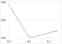
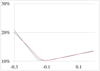
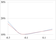
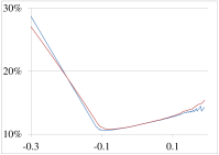
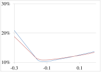
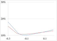
Figure 2 shows a calibration of this family of call prices to real market data. It is important to stress that there is no a priori reason why this data should resemble the call surfaces generated by this family of models. Nevertheless, although the fit is not perfect, it does seem to indicate that this modelling approach is worth pursuing further.

Figure 2. Implied volatility vs. log-moneyness for market data versus fitted density (red) with $a=3.63,b=0.0545,c=-0.0665,r=6.89$ and $y_{1}=0.234,y_{2}=0.356,y_{3}=0.439$.

4.3. A non-parametric calibration

In this section, we take a somewhat different approach. Rather than assuming that the log-concave density $f$ is a fixed parametric family, we use the results of section 4.1 to estimate $f$ non-parametrically. In particular, we assume that

$$C^{\mathrm{obs}}(\kappa,t_{1})\approx C_{f}(\kappa,\Upsilon(t_{1}))\mbox{ for all }\kappa\in\mathcal{S}_{1},$$

where now the function $f$ is unknown. Since the fit of the parametric model was reasonably good, we will set $\Upsilon(t_{1})$ to be the same value $y_{1}$ found in section 4.2.

Recall that Theorem 4.1.3 says that

$$C_{f}(e^{\varepsilon x},\varepsilon)=\varepsilon H_{f}(x)+o(\varepsilon).$$

It is straightforward to check that if $f$ satisfies as mild regularity condition as in the hypothesis of Proposition 4.1.6 then we have the slightly improved asymptotic formula

$$C_{f}(e^{\varepsilon x},\varepsilon)e^{-\varepsilon x/2}=\varepsilon H_{f}(x)+o(\varepsilon^{2}).$$

Hence, we will assume that

$$C_{f}(\kappa,y_{1})\kappa^{-1/2}\approx y_{1}H_{f}(\log\kappa/y_{1})$$

since $y_{1}$ is small. Theorem 4.1.4 tells us that

$$f\circ F^{-1}(p)\approx\frac{1}{y_{1}}\inf_{\kappa\in\mathcal{S}_{1}}[C^{\mathrm{obs}}(\kappa,t_{1})\kappa^{-1/2}+p\log(\kappa)].$$

An estimate of the density $f$ can now be computed numerically.

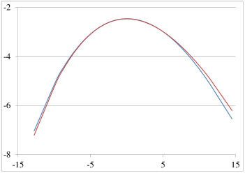
Figure 3 compares $\log f$, when estimated non-parametrically versus the calibrated parametric example from the last section. Considering the fact that the non-parametric density is estimated from the earliest maturity date, while the parametric density is calibrated using all three maturity dates, the agreement is uncanny.

Figure 3. $\log f$ estimated non-parametrically (blue), versus the parametric fit (red). Both are centred so that their maxima are at the origin.

Given that the calibrated parametric density seems to recover market date reasonably well, and that the non-parametric density agrees with parametric reasonably well, it is natural to compare the market implied volatility to that predicted by the non-parametric model. Recall that the model call surface is determined by the density $f$ and the increasing function $\Upsilon$. We have estimated $f$ from the short maturity call prices and the assumption that $\Upsilon(t_{1})=y_{1}$, where $y_{1}$ was found from the parametric calibration. However, we still need to estimate the function $\Upsilon(t_{i})$ for $i=2,3$. For a lack of a better idea, we let $\Upsilon(t_{i})=y_{i}$ for $i=2,3$ as well.

Figure 4 compares the market implied volatility (the same as in figure 2), with the implied volatility computed from the non-parametric model. Since the estimated density $f$ is not given by an explicit formula, I have used the formula in Theorem 4.1.2 to compute the call prices. Again, given that the density $f$ is estimated using only the $t_{1}$ call price curve, it is interesting that the model implied volatility for maturities $t_{2}$ and $t_{3}$ should match the market data at all.

Figure 4. Implied volatility vs. log-moneyness from market data (blue), versus the non-parametrically estimated density (red)

5. An isomorphism and lift zonoids

5.1. The isomorophism

In this section, to help understand the binary operation $\bullet$ on the space $\mathcal{C}$ we show that there is a nice isomorphism of $\mathcal{C}$ to another function space which converts the somewhat complicated operation $\bullet$ into simple function composition $\circ$.

We introduce a transformation $\hat{\ }$ on the space $\mathcal{C}$ which will be particularly useful: for $C\in\mathcal{C}$ we define a new function $\hat{C}$ on $[0,1]$ by the formula

$$\hat{C}(p)=\inf_{\kappa\geq 0}[C(\kappa)+p\kappa]\mbox{ for }0\leq p\leq 1.$$

We quickly note that the notation $\hat{\ }$ introduced here is, in fact, consistent with the prior occurrence of this notation in Section 4.1. Indeed, the connection between the transformation $\hat{\ }:\mathcal{C}\to\hat{\mathcal{C}}$ defined here and the conclusion of Theorem 4.1.4 is explored in Section 5.2 below.

Figure 5. A typical element of $\hat{\mathcal{C}}$

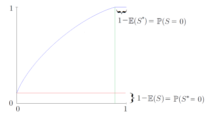
Given a call price curve $C\in\mathcal{C}$, we can immediately read off some properties of the new function $\hat{C}$. The proof is routine, and hence omitted.

Proposition 5.1.1.

Fix $C\in\mathcal{C}$ with primal representation $S$ and dual representation $S^{*}$.

1. $\hat{C}$ is non-decreasing and concave.

2. $\hat{C}$ is continuous and

   $$\hat{C}(0)=C(\infty)=1-\mathbb{E}(S)=\mathbb{P}(S^{*}=0).$$

3. For $0\leq p\leq 1$ and $\kappa\geq 0$ such that

   $$\mathbb{P}(S>\kappa)\leq p\leq\mathbb{P}(S\geq\kappa),$$

   we have

   $$\hat{C}(p)=C(\kappa)+p\kappa.$$

4. $\min\{p\geq 0:\hat{C}(p)=1\}=-C^{\prime}(0)=\mathbb{P}(S>0)=\mathbb{E}(S^{*}).$

5. $\hat{C}(p)\geq p$ for all $0\leq p\leq 1$.

Figure 5 plots the graph of a typical element $\hat{C}\in\hat{\mathcal{C}}$.

The next result identifies the image $\hat{\mathcal{C}}$ of the map $\hat{}$, and further shows that $\hat{\ }:\mathcal{C}\to\hat{\mathcal{C}}$ is a bijection:

Theorem 5.1.2.

Suppose $g:[0,1]\to[0,1]$ is continuous and concave with $g(1)=1$. Let

$$C(\kappa)=\max_{0\leq p\leq 1}[g(p)-p\kappa]\mbox{ for all }\kappa\geq 0.$$

Then $C\in\mathcal{C}$ and $g=\hat{C}.$

The above theorem is a minor variant of the Fenchel biconjugation theorem of convex analysis. See the book of Borwein & Vanderwerff [5, Theorem 2.4.4].

The following theorem explains our interest in the bijection $\hat{}$ : it converts the binary operation $\bullet$ to function composition $\circ$. A version of this result can be found in the book of Borwein & Vanderwerff [5, Exercise 2.4.31].

Theorem 5.1.3.

For $C_{1},C_{2}\in\mathcal{C}$ we have

$$\widehat{C_{1}\bullet C_{2}}=\hat{C_{1}}\circ\hat{C_{2}}$$

Proof.

By the continuity of a function $C\in\mathcal{C}$ at $\kappa=0$, we have the equivalent expression

$$\hat{C}(p)=\inf_{\kappa>0}[C(\kappa)+p\kappa]\mbox{ for }0\leq p\leq 1.$$

Hence for any $0\leq p\leq 1$ we have

$$\widehat{C_{1}\bullet C_{2}}(p) =\inf_{\kappa>0}[C_{1}\bullet C_{2}(\kappa)+p\kappa]$$

$$=\inf_{\kappa>0}\{\inf_{H>0}[C_{1}(H)+HC_{2}(\kappa/H)]+p\kappa\}$$

$$=\inf_{H>0}\{C_{1}(H)+H\inf_{\kappa>0}[C_{2}(\kappa)+p\kappa]\}$$

$$=\hat{C_{1}}\circ\hat{C_{2}}(p).$$

∎

In light of Theorem 5.1.3, Theorem 2.3.6 says that the set of conjugate functions $\hat{\mathcal{C}}$ is a semigroup with respect to function composition $\circ$, with identity element $\hat{E}(p)=p$ and absorbing element $\hat{Z}(p)=1$. The involution on $\hat{\mathcal{C}}$ induced by ^∗ is identified in Theorem 5.3.2 below.

In preparation for reproving Theorem 3.2.4 and proving Theorem 3.2.7 we identify the image of the set of functions $C_{f}$ under the isomorphism $\hat{\ }$. As the notation introduced in section 4.1 suggests, we have

$$\widehat{C_{f}(\cdot,y)}(p)=F(F^{-1}(p)+y)$$

by Theorems 4.1.2 and 5.1.2. For notational ease, we will continue to use the notation

$$\hat{C}_{f}(p,y)=\widehat{C_{f}(\cdot,y)}(p).$$

Another proof of Theorem 3.2.4.

Note that the family of functions $(\hat{C}_{f}(\cdot,y))_{y\geq 0}$ form a semigroup with respect to function composition. The result follows from applying Theorems 5.1.2 and 5.1.3. ∎

We now come to proof of Theorem 3.2.7.

Proof of Theorem 3.2.7 .

If a function $C:[0,\infty)\times[0,\infty)\to[0,1]$ satisfies the hypotheses of the theorem, then the conjugate function $\hat{C}:[0,1]\times[0,\infty)\to[0,1]$ is such that

$$\hat{C}(p,0)=p\mbox{ for all }0\leq p\leq 1$$

and satisfies the translation equation

$$\hat{C}(\hat{C}(p,y_{1}),y_{2})=\hat{C}(p,y_{1}+y_{2})\mbox{ for all }0\leq p\leq 1\mbox{ and }y_{1},y_{2}\geq 0.$$

The conclusion of the theorem is that there are only three types of solutions to the above functional equation such that $\hat{C}(\cdot,y)\in\hat{\mathcal{C}}$ for all $y>0$:

1. $\hat{C}(p,y)=p$ for all $0\leq p\leq 1$ and $y>0$,

2. $\hat{C}(p,y)=1$ for all $0\leq p\leq 1$ and $y>0$,

3. $\hat{C}(p,y)=F(F^{-1}(p)+y)$ for all $0\leq p\leq 1$ and $y>0$ where $F(z)=\int_{-\infty}^{z}f(x)dx$ and $f$ is a log-concave probability density.

Once we have ruled out cases (1) and (2), we can appeal to the result of Cherny & Filipović [9]: concave solutions of the translation equation on $[0,1]$ are of the form $G^{-1}(G(\cdot)+y)$ where

$$G(p)=\int_{p_{0}}^{p}\frac{dq}{\hat{H}(q)}$$

for a positive concave function $\hat{H}$ and fixed $0<p_{0}<1$. Note that for $0<p<1$ the integral is well-defined and finite as $\hat{H}$ is positive and continuous by concavity. Let $L=G(0)$ and $R=G(1)$, and define a function $F:[L,R]\to[0,1]$ as the inverse function $F=G^{-1}$, and extend $F$ to all of $\mathbb{R}$ by $F(x)=0$ for $x\leq L$ and $F(x)=1$ for $x\geq R$. Note that we can compute the derivative as

$$F^{\prime}(x)=\frac{1}{G^{\prime}\circ G^{-1}(x)}=\hat{H}(F(x))\mbox{ for all }x\in\mathbb{R}.$$

Setting $f=F^{\prime}$, we have $\hat{H}=f\circ F^{-1}$. Since $\hat{H}$ is concave, Bobkov’s result Proposition 3.2.3 implies that $f$ is log-concave.

∎

Remark 5.1.4.

An earlier study of the translation equation without the concavity assumption can be found in the book of Aczél [1, Chapter 6.1].

5.2. Infinitesimal generators and the inf-convolution

In this section we briefly and informally discuss the connection between the binary operation $\bullet$ defined in section 2.3 and the well-known inf-convolution $\square$.

Let $f$ be a log-concave density with distribution function $F$, and let

$$\hat{C}(p,y)=F(F^{-1}(p)+y)\mbox{ for all }0\leq p\leq 1,y\geq 0.$$

The content of Theorem 3.2.7 is that, aside from the trivial and null semigroups, the only semigroups of $\hat{\mathcal{C}}$ with respect to composition are of the above form. The infinitesimal generator is given by

$$\left.\frac{\partial}{\partial y}\hat{C}(p,y)\right|_{y=0}=\hat{H}(p)\mbox{ for all }0\leq p\leq 1,$$

where $\hat{H}=f\circ F^{-1}$ and we have taken the version of $f$ which is continuous on its support $[L,R]$. Note that this equation also holds for the trivial semigroup with $\hat{H}=0$.

The key property of the function $\hat{H}$ is that it is non-negative and concave. Let

$$\hat{\mathcal{H}}=\{h:[0,1]\to[0,\infty),\mbox{ concave }\}.$$

Note that for every element of $\hat{\mathcal{H}}$, aside from $\hat{H}=0$, one can assign a unique (up to centring) log-concave density $f$ by the discussion of section 4.1.

The space $\hat{\mathcal{H}}$ is closed under addition. Furthermore, we have for every non-null one-parameter semigroup $\hat{C}$ that

$$\hat{C}(p,\varepsilon)\approx p+\varepsilon\hat{H}(p)\mbox{ for small }\varepsilon>0$$

for some $\hat{H}\in\hat{\mathcal{H}}$. Let $\hat{C}_{1}$ and $\hat{C}_{2}$ be two such semigroups. Note that

$$\hat{C}_{1}(C_{2}(p,\varepsilon),\varepsilon) \approx p+\varepsilon(\hat{H}_{1}(p)+\hat{H}_{2}(p))$$

implying that function composition near the identity element of $\hat{\mathcal{C}}$ amounts to addition in the space of generators $\hat{\mathcal{H}}$.

Similarly, let

$$\mathcal{H}=\left\{H:\mathbb{R}\to[0,\infty)\mbox{ convex with }0\leq H(x)-(-x)^{+}\leq\mbox{ const. }\right\}.$$

For $H\in\mathcal{H}$, let

$$\hat{H}(p)=\inf_{x\in\mathbb{R}}[H(x)+xp]\mbox{ for }0\leq p\leq 1.$$

One can check that $\hat{\ }$ is a bijection between the sets $\mathcal{H}$ and $\hat{\mathcal{H}}$ by a version of the Fenchel biconjugation theorem. In particular, the space $\mathcal{H}$ can be identified with the generators of one-parameter semigroups in ${\mathcal{C}}$.

Recall that the inf-convolution of two functions $f_{1},f_{2}:\mathbb{R}\to\mathbb{R}$ is defined by

$$(f_{1}\square f_{2})(x)=\inf_{y\in\mathbb{R}}[f_{1}(x-y)+f_{2}(y)]\mbox{ for }x\in\mathbb{R}.$$

The basic property of the inf-convolution (see [5, Exercise 2.3.15] for example) is that it becomes addition under conjugation:

$$\widehat{f_{1}\square f_{2}}(p) =\inf_{x\in\mathbb{R}}\inf_{y\in\mathbb{R}}[f_{1}(x-y)+f_{2}(y)+xp]$$

$$=\inf_{z\in\mathbb{R}}[f_{1}(z)+zp]+\inf_{y\in\mathbb{R}}[f_{2}(y)+yp]$$

$$=\hat{f}_{1}(p)+\hat{f}_{2}(p),$$

in analogy with Theorem 5.1.3. Since there is an exponential map lifting function addition $+$ to function composition $\circ$ in $\hat{\mathcal{C}}$, we can apply the isomorphism $\hat{\ }$ to conclude that there is an exponential map lifting inf-convolution $\square$ to the binary operation $\bullet$ in $\mathcal{C}$.

Indeed, let $C$ be a one parameter semigroup with generator $H$, so that

$$C(e^{\varepsilon x},\varepsilon)\approx\varepsilon H(x)\mbox{ for small }\varepsilon>0.$$

Letting $C_{1}$ and $C_{2}$ be two such semigroups, we have

$$C_{1}(\cdot,\varepsilon)\bullet C_{2}(\cdot,\varepsilon)(e^{\varepsilon x}) \approx\varepsilon\ \inf_{y}[H_{1}(y)+e^{\varepsilon y}H_{2}(x-y)]$$

$$\approx\varepsilon H_{1}\square H_{2}(x)$$

5.3. Lift zonoids

Finally, to see why one might want to compute the Legendre transform of a call price with respect to the strike parameter, we recall that the zonoid of an integrable random $d$-vector $X$ is the set

$$Z_{X}=\left\{\mathbb{E}[Xg(X)]\mbox{ measurable }g:\mathbb{R}^{d}\to[0,1]\right\}\subseteq\mathbb{R}^{d},$$

and that the lift zonoid of $X$ is the zonoid of the $(1+d)$-vector $(1,X)$ given by

$$\hat{Z}_{X}=\left\{(\mathbb{E}[g(X)],\mathbb{E}[Xg(X)])\mbox{ measurable }g:\mathbb{R}^{d}\to[0,1]\right\}\subseteq\mathbb{R}^{1+d}.$$

The notion of lift zonoid was introduced in the paper of Koshevoy & Mosler [25].

In the case $d=1$, the lift zonoid $\hat{Z}_{X}$ is a convex set contained in the rectangle

$$[0,1]\times[-m_{-},m_{+}].$$

where $m_{\pm}=\mathbb{E}(X^{\pm}).$ The precise shape of this set is intimately related to call and put prices as seen in the following theorem.

Theorem 5.3.1.

Let $X$ be an integrable random variable. Its lift zonoid is given by

$$\hat{Z}_{X}=\left\{(p,q):\sup_{x\in\mathbb{R}}\{px-\mathbb{E}[(x-X)^{+}]\}\leq q\leq\inf_{x\in\mathbb{R}}\{px+\mathbb{E}[(X-x)^{+}]\},\ \ 0\leq p\leq 1\right\}.$$

Note that if we let

$$\Theta(x)=\mathbb{P}(X\geq x)$$

then we have

$$\mathbb{E}[(X-x)^{+}]=\int_{x}^{\infty}\Theta(\xi)d\xi$$

by Fubini’s theorem. Also if we define the inverse function $\Theta^{-1}$ for $0<p<1$ by

$$\Theta^{-1}(p)=\inf\{x:\Theta(x)\geq p\}$$

then by a result of Koshevoy & Mosler [25, Lemma 3.1] we have

$$\hat{Z}_{X}=\left\{(p,q):\int_{1-p}^{1}\Theta^{-1}(\phi)d\phi\leq q\leq\int_{0}^{p}\Theta^{-1}(\phi)d\phi,\ \ 0\leq p\leq 1\right\}.$$

from which Theorem 5.3.1 can be proven by Young’s inequality. However since the result can be viewed as an application of the Neyman–Pearson lemma, we include a short proof for completeness.

Proof.

For any measurable function $g$ valued in $[0,1]$ and $x\in\mathbb{R}$ we have

$$Xg(X)\leq(X-x)^{+}+xg(X)$$

with equality when $g$ is such that

$$\mathbbm{1}_{(x,\infty)}\leq g\leq\mathbbm{1}_{[x,\infty)}.$$

Now suppose $(p,q)\in\hat{Z}_{X}$ so that $p=\mathbb{E}[g(X)]$ and $q=\mathbb{E}[Xg(X)]$ for some $g$. Hence, computing expectations in the inequality above yields

$$q\leq\mathbb{E}[(X-x)^{+}]+xp.$$

with equality if

$$\mathbb{P}(X>x)\leq p\leq\mathbb{P}(X\geq x).$$

By replacing $g$ with $1-g$, we see that $(p,q)\in\hat{Z}_{X}$ if and only if $(1-p,\mathbb{E}(X)-q)\in\hat{Z}_{X}$, yielding the lower bound. ∎

We remark that the explicit connection between lift zonoids and the price of call options has been noted before, for instance in the paper of Mochanov & Schmutz [29]. In the setting of this paper, given $C\in\mathcal{C}$ represented by $S$, the lift zonoid of $S$ is given by the set

$$\hat{Z}_{S}=\{(p,q):1-\hat{C}(1-p)\leq q\leq\mathbb{E}(S)-1+\hat{C}(p),\ \ 0\leq p\leq 1\}$$

We recall that a random vector $X_{1}$ is dominated by $X_{2}$ in the lift zonoid order if $\hat{Z}_{X_{1}}\subseteq\hat{Z}_{X_{2}}$. Koshevoy & Mosler [25, Theorem 5.2] noticed that in the $d=1$ case, that the lift zonoid order is exactly the convex order.

We conclude this section by exploiting Theorem 5.3.1 to obtain an interesting identity. A similar formula can be found in the paper of Hiriart-Urruty & Martínez-Legaz [17].

Theorem 5.3.2.

Given $C\in\mathcal{C}$, let

$$\hat{C}^{-1}(q)=\inf\{p\geq 0:\hat{C}(p)\geq q\}\mbox{ for all }0\leq q\leq 1.$$

Then

$$\widehat{C^{*}}(p)=1-\hat{C}^{-1}(1-p)\mbox{ for all }0\leq p\leq 1.$$

Proof.

Let $S$ be a primal representation and $S^{*}$ be a dual representation of $C$.

Note that for all $0\leq p\leq 1$ we have

$$\hat{C}(p)-\hat{C}(0)=\sup\{\mathbb{E}[Sg(S)]:g:\mathbb{R}\to[0,1]\mbox{ with }\mathbb{E}[g(S)]=p\}$$

and hence for any $0\leq q\leq 1$ we have

$$\hat{C}^{-1}(q) =\inf\{\mathbb{E}[g(S)],\ g:\mathbb{R}\to[0,1]\mbox{ with }\mathbb{E}[Sg(S)]=q-\hat{C}(0)\}$$

$$=1-\sup\{\mathbb{E}[g(S)],\ g:\mathbb{R}\to[0,1]\mbox{ with }\mathbb{E}[Sg(S)]=1-q\}$$

$$=\mathbb{P}(S>0)-\sup\{\mathbb{E}[g(S)\mathbbm{1}_{\{S>0\}}],\ g:\mathbb{R}\to[0,1]\mbox{ with }\mathbb{E}[Sg(S)\mathbbm{1}_{\{S>0\}}]=1-q\}$$

$$=\mathbb{E}(S^{*})-\sup\left\{\mathbb{E}\left[S^{*}g(S^{*})\mathbbm{1}_{\{S^{*}>0\}}\right],\ g:\mathbb{R}\to[0,1]\mbox{ with }\mathbb{E}\left[g(S^{*})\mathbbm{1}_{\{S^{*}>0\}}\right]=1-q\right\}$$

$$=1-\widehat{C^{*}}(1-q)$$

where we have used the observation that the optimal $g$ in the final maximisation problem assigns zero weight to the event $\{S^{*}=0\}$. ∎

5.4. An extension

Let $F$ be the distribution function of a log-concave density $f$ which is supported on all of $\mathbb{R}$, so that $L=-\infty$ and $R=+\infty$ in the notation of section 3. Let

$$\hat{C}_{f}(p,y)=F(F^{-1}(p)+y)\mbox{ for all }0\leq p\leq 1,y\in\mathbb{R}.$$

By Theorem 4.1.2 we have

$$\hat{C}_{f}(p,y)=\widehat{C_{f}(\cdot,y)}(p)\mbox{ for all }0\leq p\leq 1,y\geq 0.$$

It is interesting to note that the family of functions $(\hat{C}_{f}(\cdot,y))_{y\in\mathbb{R}}$ is a group under function composition, not just a semigroup. Indeed, we have

$$\hat{C}_{f}(\cdot,-y)=\hat{C}_{f}(\cdot,y)^{-1}\mbox{ for all }y\in\mathbb{R}.$$

Note that $\hat{C}_{f}(\cdot,y)$ is increasing for all $y$, is concave if $y\geq 0$ but is convex if $y<0$. In particular, when $y<0$ the function $\hat{C}_{f}(\cdot,y)$ is not the concave conjugate of a call function in $\mathcal{C}$. Unfortunately, the probabilistic or financial interpretation of the inverse is not readily apparent.

For comparison, note that for $y\geq 0$ we have by Theorem 5.3.2 that

$$\widehat{C_{f}(\cdot,-y)}(p) =\widehat{C_{f}(\cdot,y)^{*}}(p)$$

$$=1-F(F^{-1}(1-p)-y)\mbox{ for all }0\leq p\leq 1.$$

6. Acknowledgement

I would like to thank the Cambridge Endowment for Research in Finance for their support. I would also like to thank Thorsten Rheinländer for introducing me to the notion of a lift zonoid, and Monique Jeanblanc for introducing me to the notion of a lyrebird. I would like to thank the participants of the London Mathematical Finance Seminar Series and the Oberwolfach Workshop on the Mathematics of Quantitative Finance, where this work was presented. After the original submission of this work, I learned that Peter Carr and Greg Pelts [8] independently proposed modelling call price curves via their Legendre transform. I would like to thank Johannes Ruf for noticing this connection.

I would also like to thank Johannes for a useful discussion of the implication (5)$\Rightarrow$ (1) in Theorem 3.1.2. Originally, I had a complicated proof of this implication only in the discrete-time case. The original argument was similar to the construction in the proof of Theorem 2.3.2: given the implication (5) $\Rightarrow$ (2), to apply the discrete-time Itô–Watanabe decomposition to the supermartingale $S$, as in the construction of Föllmer’s exit measure. The difficulty in extending this argument to the continuous-time case is that the local martingale appearing in the continuous-time Itô–Watanabe decomposition may not be a true martingale. While discussing this technical point, Johannes inspired me to try to prove that, in fact, the stronger implication (5) $\Rightarrow$ (4) holds.

Finally, I would like to thank the referees for their useful comments on the content and presentation of this work. In particular, I thank them for encouraging me to expand section 4.

References

- [1] J. Aczél. Lectures on Functional Equations and Their Applications. Mathematics in Science and Engineering 19. Academic Press. (1966)
- [2] S. Benaim and P. Friz. Regular variation and smile asymptotics. Mathematical Finance 19(1): 1–12. (2009)
- [3] D.T. Breeden and R.H. Litzenberger. Prices of state-contingent claims implicit in option prices. The Journal of Business 51(4): 621–651. (1978)
- [4] S. Bobkov. Extremal properties of half-spaces for log-concave distributions. Annals of Probabilty 24(1): 35–48. (1996)
- [5] J.M. Borwein and J.D. Vanderwerff. Convex Functions: Constructions, Characterizations and Counterexamples. Encyclopedia of Mathematics an Its Applications 109. Cambridge University Press. (2010)
- [6] S. Boyd and L. Vandenberghe. Convex Optimization. Cambridge University Press. (2004)
- [7] P. Carr and D. Madan. A note on sufficient conditions for no arbitrage. Finance Research Letters 2: 125–130. (2005)
- [8] P. Carr and G. Pelts. Duality, deltas, and derivatives pricing. Presentation available at http://www.math.cmu.edu/CCF/CCFevents/shreve/abstracts/P.Carr.pdf (2015)
- [9] A. Cherny, D. Filipović. Concave distortion semigroups. arXiv:1104.0508 (2011)
- [10] A.M.G. Cox, D.G. Hobson. Local martingales, bubbles and option prices. Finance and Stochastics 9: 477–492. (2005)
- [11] S. De Marco, C. Hillairet, A. Jacquier. Shapes of implied volatility with positive mass at zero. SIAM Journal on Financial Mathematics 8: 709–737. (2017)
- [12] C.-O. Ewald, M. Yor. On peacocks and lyrebirds: Australian options, Brownian bridges, and the average of submartingales. Mathematical Finance 28: 536–549. (2018)
- [13] H. Föllmer. The exit measure of a supermartingale. Zeitschrift für Wahrscheinlichkeitstheorie und Verwandte Gebiete 21(2): 154–166. (1972)
- [14] J. Gatheral, A. Jacquier. Arbitrage-free SVI volatility surfaces. Quantitative Finance 14(1): 59–71. (2014)
- [15] A. Gulisashvili. Asymptotic formulas with error estimates for call pricing functions and the implied volatility at extreme strikes. SIAM Journal on Financial Mathematics 1: 609–641. (2010)
- [16] G. Guo, A. Jacquier, C. Martini, L. Neufcourt. Generalised arbitrage-free SVI volatility surfaces. SIAM Journal on Financial Mathematics 7(1): 619–641. (2016)
- [17] J-B. Hiriart-Urruty and J-E. Martínez-Legaz. New formulas for the Legendre–Fenchel transform. Journal of Mathematical Analysis and Applications. 288: 544–555 (2003)
- [18] F. Hirsh, Ch. Profeta, B. Roynette and M. Yor. Peacocks and Associated Martingales, with Explicit Constructions. Bocconi & Springer Series. (2011)
- [19] F. Hirsh and B. Roynette. A new proof of Kellerer’s theorem. ESAIM: Probability and Statistics 16: 48–60. (2012)
- [20] D. Hobson, P. Laurence, and T-H. Wang. Static-arbitrage upper bounds for the prices of basket options. Quantitative Finance 5(4): 329–342. (2005)
- [21] A. Jacquier and M. Keller-Ressel. Implied volatility in strict local martingale models. SIAM Journal on Financial Mathematics 9: 171–189. (2018)
- [22] R. Kaas, J. Dhaene, D. Vyncke, M.J. Goovaerts, M. Denuit. A simple geometry proof that comonotonic risks have the convex-largest sum. ASTIN Bulletin 32: 71–80. (2002)
- [23] I. Karatzas. Lectures on the Mathematics of Finance. CRM Monograph Series, American Mathematical Society. (1997)
- [24] H.G. Kellerer. Markov-Komposition und eine Anwendung auf Martingale. Mathematische Annalen 198: 99–122. (1972)
- [25] G. Koshevoy and K. Mosler. Lift zonoids, random convex hulls and the variability of random vectors. Bernoulli 4: 377–399. (1998)
- [26] A.M. Kulik and T.D. Tymoshkevych. Lift zonoid order and functional inequalities. Theory of Probability and Mathematical Statistics 89: 83–99. (2014)
- [27] M. Kulldorff. Optimal control of favorable games with a time-limit. SIAM Journal on Control and Optimization 31(1): 52–69. (1993)
- [28] R. Lee. The moment formula for implied volatility at extreme strikes. Mathematical Finance 14(3): 469–480. (2004)
- [29] I. Molchanov and M. Schmutz. Multivariate extension of put-call symmetry. SIAM Journal on Financial Mathematics 1(1): 396–426. (2010)
- [30] V. Strassen. The existence of probability measures with given marginals. Annals of Mathematical Statistics 36: 423–439. (1965)
- [31] M.R. Tehranchi. Uniform bounds on Black–Scholes implied volatility. SIAM Journal on Financial Mathematics 7(1): 893–916. (2016)
- [32] M.R. Tehranchi. Arbitrage theory without a numéraire. Available at http://arxiv.org/abs/1410.2976 (2015)
- [33] S.S. Wang. A class of distortion operators for pricing financial and insurance risks. The Journal of Risk and Insurance 67(1): 15–36. (2000)