3D $B_{2}$ Model for Radiative Transfer Equation
Part I: Modelling

Abstract

We extend to three-dimensional space the approximate $M_{2}$ model for the slab geometry studied in [3]. The $B_{2}$ model therein, as a special case of the second order extended quadrature method of moments (EQMOM), is proved to be globally hyperbolic. The model we propose here extends EQMOM to multiple dimensions following the idea to approximate the maximum entropy closure for the slab geometry case. Like the $M_{2}$ closure, the ansatz of the new model has the capacity to capture both isotropic and beam-like solutions. Also, the new model has fluxes in closed-form; thus, it is applicable to practical numerical simulations. The rotational invariance, realizability, and hyperbolicity of the model are studied.

Keywords: Radiative transfer, moment model, maximum entropy closure

1 Introduction

The radiative transfer equations describe the transportation of light in a medium [14]. They are kinetic equations, and the unknown is the specific intensity of photons. The specific intensity is a function of time, spatial coordinates, frequency, and angular variables. The moment method is an efficient approach for reducing the computation cost brought about by the high-dimensionality of variables of kinetic equations.

Moments are obtained by integrating the specific intensity against monomials of the angular variables. In many applications, the quantities of interest are the few lowest order moments. Therefore moments are good choices for discretizing the angular variables. However, moment systems are not closed. Closing the system by specifying a constitutive relationship is known as the moment-closure problem. One approach towards moment-closure is to recover the angular dependence of the specific intensity from the known moments. The reconstructed specific intensity is called an ansatz. Ideally, the ansatz should be non-negative for all moments which can be generated by a non-negative distribution. Also, one would like the system to be hyperbolic since hyperbolicity is necessary for the local well-posedness of Cauchy problem. Other natural requirements include that the ansatz satisfies rotational invariance and reproduces the isotropic distribution at equilibrium. Numerous forms of ansätze have been studied in the literature [14, 12]. Yet, in multi-dimensional cases, the maximum entropy method, referred to as the $M_{n}$ model, is perhaps the only method known so far to have both realizability and global hyperbolicity [5]. However, the flux functions of the maximum entropy method are generally not explicit , so numerically computing such models involve solving highly nonlinear and probably ill-conditioned optimization problems frequently. There have been continuous efforts on speeding up the computation process [2, 1, 7]. Recently, there are also attempts in deriving closed-form approximations of the maximum entropy closure in order to avoid the expensive computations. For 1D cases, an approximation to the $M_{n}$ models using the Kershaw closure is given in [15]. For multi-dimensional cases, a model based on directly approximating the closure relations of the $M_{1}$ and $M_{2}$ methods is proposed in [13]. Our work in this paper also aims at constructing closed-form approximations of the maximum entropy model. Like [13], we seek a closed-form approximation to the $M_{2}$ method in 3D. But unlike [13], we derive our model from an ansatz with some similarity to that of the $M_{2}$ model.

In a previous study [3], we analyzed the second order extended quadrature method of moments (EQMOM) introduced in [16] which we call the $B_{2}$ model. In this work, we propose an approximation of the $M_{2}$ model in 3D space by extending the $B_{2}$ model studied in [3] to 3D. The reason for this approach is that the $B_{2}$ ansatz shares the following properties with the $M_{2}$ ansatz:

1. it interpolates smoothly between isotropic and Dirac distribution functions;

2. it captures anisotropy in opposite directions.

The $B_{2}$ closure in [3] is for slab geometries. Preserving rotational invariance when extending it to 3D space is non-trivial. We use the sum of the axisymmetric $B_{2}$ ansätze in three mutually orthogonal directions as the ansatz for a second order moment model in 3D space. This new model is referred to as the 3D $B_{2}$ model. The consistency of known moments requires the three mutually orthogonal directions to be the three eigenvectors of the second-order moment matrix. We point out that there are three free parameters in the ansatz of the 3D $B_{2}$ model after the consistency of known moments is fulfilled. These parameters are specified as functions of the first-order moments and the eigenvalues of the second-order moment matrix. We prove that the 3D $B_{2}$ model is rotationally invariant. The region where the model possesses a non-negative ansatz is illustrated, as well as the hyperbolicity region of the model with vanished first-order moment. Though far from perfect, the 3D $B_{2}$ model shares some important features of the $M_{2}$ closure. Also, the model has explicit flux functions, making it very convenient for numerical simulations.

The rest of this paper is organized as follows. In Section 2 we recall the basics of moment models, and briefly, introduce the $M_{2}$ method as well as the $B_{2}$ model for 1D slab geometry. In Section 3 we propose the 3D $B_{2}$ model. In Section 4 we analyze its properties. Finally, in Section 5 we summarize and discuss future work.

2 Preliminaries

The specific intensity $I(t,\mathbf{r},\nu,\boldsymbol{\Omega})$ is governed by the radiative transfer equation

$$\dfrac{1}{c}\dfrac{\partial I}{\partial t}+\boldsymbol{\Omega}\cdot\nabla I=\mathcal{C}(I),$$ (1)

where $c$ is the speed of light. The variables in the equation are time $t\in\mathbb{R}^{+}$, the spatial coordinates $\mathbf{r}=(x,y,z)\in\mathbb{R}^{3}$, the angular variables $\boldsymbol{\Omega}=\left(\Omega_{x},\Omega_{y},\Omega_{z}\right)\in\mathbb{S}^{2}$, and frequency $\nu\in\mathbb{R}^{+}$. The right-hand side $\mathcal{C}(I)$ describes the interactions between photons and the background medium and are not the focus of this paper. A typical right-hand side takes the form

$$\mathcal{C}(I)=-\sigma_{a}I(\boldsymbol{\Omega})-\sigma_{s}\left(I(\boldsymbol{\Omega})-\frac{1}{4\pi}\int_{\mathbb{S}^{2}}I(\boldsymbol{\Omega})\,{\rm d}\boldsymbol{\Omega}\right),$$

where $\sigma_{a}$ and $\sigma_{s}$ are constant parameters. We introduce the moment method in the context of second order models. Let

$$\begin{array}[]{rllll}\mathbf{v}=[&1,&&&\\[5.69054pt] &(\boldsymbol{\Omega}\cdot\mathbf{e}_{x}),&(\boldsymbol{\Omega}\cdot\mathbf{e}_{y}),&(\boldsymbol{\Omega}\cdot\mathbf{e}_{z}),&\\[5.69054pt] &(\boldsymbol{\Omega}\cdot\mathbf{e}_{x})^{2},&(\boldsymbol{\Omega}\cdot\mathbf{e}_{x})(\boldsymbol{\Omega}\cdot\mathbf{e}_{y}),&(\boldsymbol{\Omega}\cdot\mathbf{e}_{x})(\boldsymbol{\Omega}\cdot\mathbf{e}_{z}),&\\ &&(\boldsymbol{\Omega}\cdot\mathbf{e}_{y})^{2},&(\boldsymbol{\Omega}\cdot\mathbf{e}_{y})(\boldsymbol{\Omega}\cdot\mathbf{e}_{z})&]^{T}.\end{array}$$ (2)

Use $\mathbf{e}_{x}$, $\mathbf{e}_{y}$ and $\mathbf{e}_{z}$ to denote the unit vectors along the coordinate axes. Define

$$\left\langle\psi\right\rangle:=\int_{\mathbb{S}^{2}}\psi(\nu,\boldsymbol{\Omega})\,\,{\rm d}\boldsymbol{\Omega}.$$

Multiplying equation (1) by the vector $\mathbf{v}$ defined in (2) and integrating over the angular variables give

$$\dfrac{1}{c}\dfrac{\partial\left\langle\mathbf{v}I\right\rangle}{\partial t}+\dfrac{\partial\left\langle\Omega_{x}\mathbf{v}I\right\rangle}{\partial x}+\dfrac{\partial\left\langle\Omega_{y}\mathbf{v}I\right\rangle}{\partial y}+\dfrac{\partial\left\langle\Omega_{z}\mathbf{v}I\right\rangle}{\partial z}=\left\langle\mathbf{v}\mathcal{C}(I)\right\rangle.$$ (3)

In system (3), the time evolution of second-order moments relies on third-order moments. Therefore (3) is not a closed system. If we approximate the third-order moments in (3) using lower order moments, we could get a closed system. Let

$$E^{0}\simeq\left\langle I\right\rangle,\quad\mathbf{E}^{1}\simeq\left\langle\boldsymbol{\Omega}I\right\rangle,\quad\boldsymbol{\mathit{E}}^{2}\simeq\left\langle\boldsymbol{\Omega}\otimes\boldsymbol{\Omega}I\right\rangle,\quad\boldsymbol{\mathit{E}}^{3}\simeq\left\langle\boldsymbol{\Omega}\otimes\boldsymbol{\Omega}\otimes\boldsymbol{\Omega}I\right\rangle.$$

A closed system of equations has the form

$$\begin{split}&\dfrac{1}{c}\dfrac{\partial E^{0}}{\partial t}+\nabla\cdot\mathbf{E}^{1}=r^{0}(E^{0},\mathbf{E}^{1},\boldsymbol{\mathit{E}}^{2}),\\ &\dfrac{1}{c}\dfrac{\partial\mathbf{E}^{1}}{\partial t}+\nabla\cdot\boldsymbol{\mathit{E}}^{2}=\mathbf{r}^{1}(E^{0},\mathbf{E}^{1},\boldsymbol{\mathit{E}}^{2}),\\ &\dfrac{1}{c}\dfrac{\partial\boldsymbol{\mathit{E}}^{2}}{\partial t}+\nabla\cdot\left[\boldsymbol{\mathit{E}}^{3}(E^{0},\mathbf{E}^{1},\boldsymbol{\mathit{E}}^{2})\right]=\boldsymbol{\mathit{r}}^{2}(E^{0},\mathbf{E}^{1},\boldsymbol{\mathit{E}}^{2}).\end{split}$$ (4)

The choice of $\boldsymbol{\mathit{E}}^{3}$, $r^{0}$, $\mathbf{r}^{1}$, and $\boldsymbol{\mathit{r}}^{2}$ specify a closure. The system (4) is a second order moment model. The following properties of a moment model concern us the most, which were frequently discussed in the literature.

• Rotational invariance: Consider a conservation law in multi-dimensions,

  $$\dfrac{\partial\mathbf{U}}{\partial t}+\tsum\slimits@\limits_{i=1}^{D}\dfrac{\partial\mathbf{F}_{i}(\mathbf{U})}{\partial x_{i}}=0.$$ (5)

  It satisfies rotational invariance if for any unit vector $\mathbf{n}=(n_{1},\@cdots,n_{D})^{T}\in\mathbb{R}^{D}$, there exists a matrix $\mathbb{T}$ depending on $\mathbf{n}$, such that

  $$\tsum\slimits@\limits_{i=1}^{D}n_{i}\mathbf{F}_{i}(\mathbf{U})=\mathbb{T}^{-1}\mathbf{F}_{1}(\mathbb{T}\mathbf{U}).$$

• Hyperbolicity: Let $\boldsymbol{\mathrm{J}}_{i}$ be the Jacobian matrix of the flux function $\mathbf{F}_{i}$ in equation (5). The system (5) is hyperbolic if for any unit vector $\mathbf{n}\in\mathbb{R}^{D}$, $\tsum\slimits@\limits_{i=1}^{D}n_{i}\boldsymbol{\mathrm{J}}_{i}$ is real diagonalizable.

• Realizability: The realizability domain is defined as moments which could be generated by a nonnegative distribution function [9]. A closure is said to be realizable if the higher order moments it closes belong to the realizability domain.

  For one dimensional problem, [4] gives necessary and sufficient conditions for realizability. Its results cover moments of arbitrary order. For multi-dimensional case, only the conditions for the first and second order models are currently known [10], while the conditions for moments of higher order remain open problems.

The maximum entropy models are equipped with all the properties mentioned above. For detailed discussions we refer to [9, 11, 5]. We review the principles for deriving the maximum entropy models by taking the second order case as an example. It is called the $M_{2}$ model. Solve the following constrained variational minimization problem

$$\begin{split}\operatorname*{minimize}\>\>&H(I)\\ \operatorname*{subject~{}to}\>\>&\left\langle I\right\rangle=E^{0},\left\langle\boldsymbol{\Omega}I\right\rangle=\mathbf{E}^{1},\text{and }\left\langle\boldsymbol{\Omega}\otimes\boldsymbol{\Omega}I\right\rangle=\boldsymbol{\mathit{E}}^{2}\end{split}$$ (6)

where $H(I)$ is the Bose-Einstein entropy

$$H(I):=\left\langle\frac{2k_{B}\nu^{2}}{c^{3}}\left(\chi I\log\left(\chi I\right)-\left(\chi I+1\right)\log\left(\chi I+1\right)\right)\right\rangle,$$ (7)

where $\chi=\dfrac{c^{2}}{2\middlebar{h}\nu^{3}}$. This gives us an ansatz

$$\hat{I}_{M}(\nu,\boldsymbol{\Omega})=\dfrac{1}{\chi}\left(\exp\left(-\dfrac{\middlebar{h}\nu}{k_{B}}\boldsymbol{\alpha}\cdot\mathbf{v}\right)-1\right)^{-1},$$ (8)

where $\boldsymbol{\alpha}\cdot\mathbf{v}$ is a second order polynomial of $\boldsymbol{\Omega}\in\mathbb{S}^{2}$. The parameters $\boldsymbol{\alpha}$ is the unique vector such that

$$\left\langle\hat{I}_{M}\right\rangle=E^{0},\quad\left\langle\boldsymbol{\Omega}\hat{I}_{M}\right\rangle=\mathbf{E}^{1},\text{and}\quad\left\langle\boldsymbol{\Omega}\otimes\boldsymbol{\Omega}\hat{I}_{M}\right\rangle=\boldsymbol{\mathit{E}}^{2}.$$

The $M_{2}$ method is defined by taking

$$\begin{array}[]{ll}\boldsymbol{\mathit{E}}^{3}:=\left\langle\boldsymbol{\Omega}\otimes\boldsymbol{\Omega}\otimes\boldsymbol{\Omega}\hat{I}_{M}\right\rangle,&r^{0}:=\left\langle\mathcal{C}(\hat{I}_{M})\right\rangle,\\ \mathbf{r}^{1}:=\left\langle\boldsymbol{\Omega}\mathcal{C}(\hat{I}_{M})\right\rangle,&\boldsymbol{\mathit{r}}^{2}:=\left\langle\boldsymbol{\Omega}\otimes\boldsymbol{\Omega}\mathcal{C}(\hat{I}_{M})\right\rangle.\end{array}$$ (9)

in (4).

However, the $M_{2}$ closure is not given explicitly, so (9) has to be computed by solving the optimization problem (6) numerically. The numerical optimization at each time step for all spatial grid is extremely expensive.

Recent work [13] proposes an approximation of the $M_{2}$ method in multi-dimensions by directly approximating its closure relation, though the corresponding ansatz to the closure is not clarified. We adopt the approach of constructing an ansatz to approximate the $M_{2}$ ansatz, then the closure relation is given naturally as in (9).

In a previous work [3], we examined the properties of second order extended quadrature method of moments (EQMOM) proposed in [16] in slab geometry, and the model was referred as the $B_{2}$ model. In EQMOM, the ansatz $\hat{I}$ is reconstructed by a combination of beta distributions. The beta distribution on $[-1,1]$ is given by

$$\mathcal{F}(\mu;\gamma,\delta)=\frac{1}{2\boldsymbol{B}(\xi,\eta)}\left(\frac{1+\mu}{2}\right)^{\xi-1}\left(\frac{1-\mu}{2}\right)^{\eta-1},\quad\xi=\frac{\gamma}{\delta},\quad\eta=\frac{1-\gamma}{\delta}.$$

where $\boldsymbol{B}(\xi,\eta)$ is the beta function. For the $B_{2}$ model in 1D slab geometry, the ansatz is taken as

$$w\mathcal{F}(\mu;\gamma,\delta)$$

where the parameters $w$, $\gamma$, and $\delta$ are given by consistency to the known moments.

We found that the 1D $B_{2}$ model shares the key features of the $M_{2}$ model in slab geometry, including existence of non-negative ansatz and therefore realizability, as well as global hyperbolicity. It is the focus of this paper to extend the 1D $B_{2}$ model to three-dimensional case.

Our motivation to this extension is based on observing a common attribute between the $B_{2}$ and the $M_{2}$ ansatz in 1D slab geometry. Both ansatz can exactly recover the isotropic distribution, and at the same time, give a combination of Dirac functions on the boundary of the realizability domain. Dirac functions could not be recovered by the standard spectral method which has a polynomial as an ansatz. It has been pointed out that the inability to capture anisotropy is a drawback of the standard spectral method [6].

In three-dimensional space, the anisotropy of the specific intensity could come in orthogonal directions. For example, we consider a setup similar to the double beam problem discussed in [13] . For the region $[x,y]\in[-1,1]\times[-1,1]$, consider equation (1) with the right-hand side chosen as isotropic scattering (which means $\sigma_{\mathrm{s}}$ is a non-negative constant):

$$\mathcal{C}(I)=\sigma_{\mathrm{s}}\left(-I+\dfrac{1}{4\pi}\left\langle I\right\rangle\right).$$

Laser beams are imposed as boundary inflow from orthogonal directions: $I=\delta(\boldsymbol{\Omega}\cdot\mathbf{e}_{x}-1)$ on the boundary $x=-1$, and $I=\delta(\boldsymbol{\Omega}\cdot\mathbf{e}_{y}-1)$ on the boundary $y=-1$.

For the extreme case when the medium is vacuum and $\sigma_{\mathrm{s}}=0$, the exact solution for any $ct>2$ is

$$I=\delta(\boldsymbol{\Omega}\cdot\mathbf{e}_{x}-1)+\delta(\boldsymbol{\Omega}\cdot\mathbf{e}_{y}-1).$$ (10)

It is pointed out in [13] that the $M_{2}$ ansatz is able to exactly reproduce the distribution in (10) from the moments. We aim to construct an ansatz that can capture anisotropy in orthogonal directions, like the $M_{2}$ ansatz.

For non-vanishing scattering, the steady-state solution of the above problem is an isotropic distribution. For any period before steady-state is reached, the exact specific intensity $I$ should be somewhere between double beams, as in (10), and isotropic. The ansatz of the $M_{2}$ model provides a smooth interpolation between these two extremes, giving it an advantage in simulating such problems. We aim to propose an ansatz with similar features. This will be discussed in the following sections.

3 3D $B_{2}$ Model

For second order models, which are the subject of this paper, the set of realizable moments as given in [10] is

$$\begin{split}\mathcal{M}=\Big{\{}&\left(E^{0},\mathbf{E}^{1},\boldsymbol{\mathit{E}}^{2}\right)\in\mathbb{R}\times\mathbb{R}^{3}\times\mathbb{R}^{3\times 3},~{}~{}\text{s.t.}~{}~{}0<E^{0}=\mathrm{Trace}(\boldsymbol{\mathit{E}}^{2}),\\ &\|\mathbf{E}^{1}\|\leq E^{0},\,~{}~{}\text{and}~{}~{}E^{0}\boldsymbol{\mathit{E}}^{2}-\mathbf{E}^{1}\otimes\mathbf{E}^{1}~{}~{}\text{symmetric non-negative}\Big{\}}.\end{split}$$ (11)

It is also referred to as the realizability domain. Our goal is to reconstruct an ansatz of the specific intensity given moments within $\mathcal{M}$.

We take the summation of three axisymmetric distributions as the ansatz for the specific intensity:

$$\hat{I}_{B}(\boldsymbol{\Omega})=\tsum\slimits@_{i=1}^{3}\dfrac{1}{2\pi}w_{i}f(\boldsymbol{\Omega}\cdot\mathbf{R}_{i};\gamma_{i},\delta_{i}),$$ (12)

where $\mathbf{R}_{i}$ are three mutually orthogonal unit vectors. We assume that the matrix $\boldsymbol{\mathit{R}}=\left[\mathbf{R}_{1},\mathbf{R}_{2},\mathbf{R}_{3}\right]$ satisfy $\mathit{det}(\boldsymbol{\mathit{R}})=1$. It is also assumed that $f(\mu;\gamma,\delta)$ is a non-negative function of $\mu$ with two shape parameters $\gamma$ and $\delta$, and $\displaystyle\int_{-1}^{1}f(\mu;\gamma,\delta)\,{\rm d}\mu=1$. All the parameters in the ansatz, including $\mathbf{R}_{i}$, $w_{i}$, $\gamma_{i}$, and $\delta_{i}$, $i=1,2,3$, are functions of known moments and are independent of $\boldsymbol{\Omega}$. We first discuss the properties of (12) for any arbitrary non-negative function $f(\mu;\gamma,\delta)$ whose integral over $\mu\in[-1,1]$ is one. To simplify the computing process in discussing the consistency conditions, we first make the following observation which will be used later.

Lemma 3.1.

For any permutation $l,m,k$ of $1,2,3$, $\forall n_{l},n_{m},n_{k}\in\mathbb{N}$, we have

$$\left\langle(\boldsymbol{\Omega}\cdot\mathbf{R}_{l})^{n_{l}}(\boldsymbol{\Omega}\cdot\mathbf{R}_{m})^{n_{m}}(\boldsymbol{\Omega}\cdot\mathbf{R}_{k})^{n_{k}}f(\boldsymbol{\Omega}\cdot\mathbf{R}_{k};\gamma_{k},\delta_{k})\right\rangle=$$

$$\qquad\qquad\qquad\left\{\begin{array}[]{l}0,~{}~{}\text{if either }~{}n_{l}\text{ or }n_{m}\text{ is odd},\\[11.38109pt] 2\pi\int_{-1}^{1}\mu^{n_{k}}f(\mu;\gamma_{k},\delta_{k})\,{\rm d}\mu,~{}~{}\text{if }n_{l}=n_{m}=0,\\[11.38109pt] \pi\int_{-1}^{1}(1-\mu^{2})\mu^{n_{k}}f(\mu;\gamma_{k},\delta_{k})\,{\rm d}\mu,~{}~{}\text{if }n_{l}=2,~{}n_{m}=0.\end{array}\right.$$

Proof.

Note that $f(\boldsymbol{\Omega}\cdot\mathbf{R}_{k};\gamma_{k},\delta_{k})$ is an axisymmetric function with $\mathbf{R}_{k}$ as its symmetric axis. Once $\mathbf{R}_{i}$, $i=1,2,3$, are given, the value of

$$\int_{\mathbb{S}^{2}}(\boldsymbol{\Omega}\cdot\mathbf{R}_{l})^{n_{l}}(\boldsymbol{\Omega}\cdot\mathbf{R}_{m})^{n_{m}}(\boldsymbol{\Omega}\cdot\mathbf{R}_{k})^{n_{k}}f(\boldsymbol{\Omega}\cdot\mathbf{R}_{k};\gamma_{k},\delta_{k})\,{\rm d}\boldsymbol{\Omega},$$

can be calculated conveniently by setting $\mathbf{R}_{k}$ as coordinate axes. Below, we will repeatedly use this method to compute the moments.

Set the $z$-axis to be aligned to $\mathbf{R}_{k}$, the $x$-axis to be aligned to $\mathbf{R}_{l}$, and the $y$-axis aligned to $\mathbf{R}_{m}$. Then

$$\begin{split}&\int_{\mathbb{S}^{2}}(\boldsymbol{\Omega}\cdot\mathbf{R}_{l})^{n_{l}}(\boldsymbol{\Omega}\cdot\mathbf{R}_{m})^{n_{m}}(\boldsymbol{\Omega}\cdot\mathbf{R}_{k})^{n_{k}}f(\boldsymbol{\Omega}\cdot\mathbf{R}_{k};\gamma_{k},\delta_{k})\,{\rm d}\boldsymbol{\Omega}\\ =&\int_{0}^{\pi}\left(\int_{0}^{2\pi}(\sin\theta\cos\phi)^{n_{l}}(\sin\theta\sin\phi)^{n_{m}}(\cos\theta)^{n_{k}}f(\cos\theta;\gamma_{k},\delta_{k})\,{\rm d}\phi\right)\sin\theta\,{\rm d}\theta\\ =&\int_{0}^{\pi}(\sin\theta)^{n_{l}+n_{m}}(\cos\theta)^{n_{k}}f(\cos\theta;\gamma_{k},\delta_{k})\sin\theta\,{\rm d}\theta\int_{0}^{2\pi}(\cos\phi)^{n_{l}}(\sin\phi)^{n_{m}}\,{\rm d}\phi.\end{split}$$

Assume that $n_{l}$ is odd, let $n_{l}=2j+1$. Then

$$\begin{split}&\int_{0}^{2\pi}(\cos\phi)^{n_{l}}(\sin\phi)^{n_{m}}\,{\rm d}\phi\\ =&\int_{0}^{2\pi}(\cos\phi)^{2j+1}(\sin\phi)^{n_{m}}\,{\rm d}\phi\\ =&\int_{0}^{2\pi}(1-(\sin\phi)^{2})^{j}(\sin\phi)^{n_{m}}\,{\rm d}\sin\phi\\ =&~{}0.\end{split}$$

Other cases are proved similarily.

To calculate

$$\dfrac{1}{2\pi}\int_{\mathbb{S}^{2}}(\boldsymbol{\Omega}\cdot\mathbf{R}_{k})^{n_{k}}f(\boldsymbol{\Omega}\cdot\mathbf{R}_{k};\gamma_{k},\delta_{k})\,{\rm d}\boldsymbol{\Omega},$$

we set up the coordinate system such that $\mathbf{R}_{k}$ is aligned to the $z$-axis. Let $\mu=\boldsymbol{\Omega}\cdot\mathbf{R}_{k}$, then

$$\begin{split}&\dfrac{1}{2\pi}\int_{\mathbb{S}^{2}}(\boldsymbol{\Omega}\cdot\mathbf{R}_{k})^{n_{k}}f(\boldsymbol{\Omega}\cdot\mathbf{R}_{k};\gamma_{k},\delta_{k})\,{\rm d}\boldsymbol{\Omega}\\ =&\dfrac{1}{2\pi}\int_{0}^{\pi}\left(\int_{0}^{2\pi}(\cos\theta)^{n_{k}}f(\cos\theta;\gamma_{k},\delta_{k})\,{\rm d}\phi\right)\sin\theta\,{\rm d}\theta\\ =&\int_{0}^{\pi}(\cos\theta)^{n_{k}}f(\cos\theta;\gamma_{k},\delta_{k})\sin\theta\,{\rm d}\theta\\ =&\int_{-1}^{1}\mu^{n_{k}}f(\mu;\gamma_{k},\delta_{k})\,{\rm d}\mu.\end{split}$$

If we let the $z$-axis to be aligned to $\mathbf{R}_{k}$ and the $y$-axis to be aligned to $\mathbf{R}_{l}$, we have

$$\begin{split}&\dfrac{1}{2\pi}\int_{\mathbb{S}^{2}}(\boldsymbol{\Omega}\cdot\mathbf{R}_{l})^{2}(\boldsymbol{\Omega}\cdot\mathbf{R}_{k})^{n_{k}}f(\boldsymbol{\Omega}\cdot\mathbf{R}_{k};\gamma_{k},\delta_{k})\,{\rm d}\boldsymbol{\Omega}\\ =&\dfrac{1}{2\pi}\int_{0}^{\pi}\left(\int_{0}^{2\pi}(\sin\theta\sin\phi)^{2}(\cos\theta)^{n_{k}}f(\cos\theta;\gamma_{k},\delta_{k})\,{\rm d}\phi\right)\sin\theta\,{\rm d}\theta,\\ =&\dfrac{1}{2\pi}\int_{0}^{\pi}(\sin\theta)^{2}(\cos\theta)^{n_{k}}f(\cos\theta;\gamma_{k},\delta_{k})\sin\theta\,{\rm d}\theta\int_{0}^{2\pi}(\sin\phi)^{2}\,{\rm d}\phi\\ =&\dfrac{1}{2}\int_{-1}^{1}(1-\mu^{2})\mu^{n_{k}}f(\mu;\gamma_{k},\delta_{k})\,{\rm d}\mu.\end{split}$$

Summarizing the results from the above three cases completes the proof of this lemma. ∎

Take $\mathbf{v}$ as defined in (2), the moments of interest are

$$\mathbf{E}=[E^{0},E^{1}_{1},E^{1}_{2},E^{1}_{3},E^{2}_{11},E^{2}_{12},E^{2}_{13},E^{2}_{22},E^{2}_{23}]^{T}=\int_{\mathbb{S}^{2}}\mathbf{v}\hat{I}_{B}\,{\rm d}\boldsymbol{\Omega}.$$

The moment system based on the ansatz (12) is derived as

$$\dfrac{\partial\mathbf{E}}{\partial t}+\dfrac{\partial\mathbf{f}_{x}(\mathbf{E})}{\partial x}+\dfrac{\partial\mathbf{f}_{y}(\mathbf{E})}{\partial y}+\dfrac{\partial\mathbf{f}_{z}(\mathbf{E})}{\partial z}=\mathbf{r}(\mathbf{E}),$$ (13)

where

$$\begin{split}&\mathbf{f}_{x}=[E^{1}_{1},E^{2}_{11},E^{2}_{12},E^{2}_{13},E^{3}_{111},E^{3}_{112},E^{3}_{113},E^{3}_{122},E^{3}_{123}]^{T}=\int_{\mathbb{S}^{2}}(\boldsymbol{\Omega}\cdot\mathbf{e}_{x})\mathbf{v}\hat{I}_{B}\,{\rm d}\boldsymbol{\Omega},\\ &\mathbf{f}_{y}=[E^{1}_{2},E^{2}_{21},E^{2}_{22},E^{2}_{23},E^{3}_{211},E^{3}_{212},E^{3}_{213},E^{3}_{222},E^{3}_{223}]^{T}=\int_{\mathbb{S}^{2}}(\boldsymbol{\Omega}\cdot\mathbf{e}_{y})\mathbf{v}\hat{I}_{B}\,{\rm d}\boldsymbol{\Omega},\\ &\mathbf{f}_{z}=[E^{1}_{3},E^{2}_{31},E^{2}_{32},E^{2}_{33},E^{3}_{311},E^{3}_{312},E^{3}_{313},E^{3}_{322},E^{3}_{323}]^{T}=\int_{\mathbb{S}^{2}}(\boldsymbol{\Omega}\cdot\mathbf{e}_{z})\mathbf{v}\hat{I}_{B}\,{\rm d}\boldsymbol{\Omega},\end{split}$$

and $\mathbf{r}(\mathbf{E})$ is calculated from the scattering term, which is out of the scope of our interests in this paper.

The parameters $\mathbf{R}_{i}$, $w_{i}$, $\gamma_{i}$, and $\delta_{i}$ have to satisfy the consistency conditions:

$$E^{0}=\left\langle\hat{I}_{B}\right\rangle,\quad\mathbf{E}^{1}=\left\langle\boldsymbol{\Omega}\hat{I}_{B}\right\rangle,\quad\mbox{and}\quad\boldsymbol{\mathit{E}}^{2}=\left\langle\boldsymbol{\Omega}\otimes\boldsymbol{\Omega}\hat{I}_{B}\right\rangle.$$ (14)

The vectors $\mathbf{R}_{i}$ in (12) are determined by the consistency conditions (14) instantly, as shown in the following lemma.

Lemma 3.2.

The consistency constraints (14) require that $\mathbf{R}_{j}$, $j=1,2,3$, be the eigenvectors of $\boldsymbol{\mathit{E}}^{2}$.

Proof.

Let $\boldsymbol{\mathit{R}}=\left[\mathbf{R}_{1},\mathbf{R}_{2},\mathbf{R}_{3}\right]$. As $\boldsymbol{\mathit{R}}$ is an orthogonal matrix, we have $\boldsymbol{\mathit{R}}^{-1}=\boldsymbol{\mathit{R}}^{T}$. To prove the lemma, it suffices to show that

$$\mathbf{R}_{j}^{T}\boldsymbol{\mathit{E}}^{2}\mathbf{R}_{i}=\left\langle(\boldsymbol{\Omega}\cdot\mathbf{R}_{j})(\boldsymbol{\Omega}\cdot\mathbf{R}_{i})\hat{I}_{B}\right\rangle=0,\quad\text{if}~{}j\mathrel{\mathchoice{\ooalign{$\hfil\displaystyle/\hfil$\crcr$\displaystyle=$}}{\ooalign{$\hfil\textstyle/\hfil$\crcr$\textstyle=$}}{\ooalign{$\hfil\scriptstyle/\hfil$\crcr$\scriptstyle=$}}{\ooalign{$\hfil\scriptscriptstyle/\hfil$\crcr$\scriptscriptstyle=$}}}i.$$ (15)

The reason is that (15) would indicate that $\boldsymbol{\mathit{R}}^{-1}\boldsymbol{\mathit{E}}^{2}\boldsymbol{\mathit{R}}$ is a diagonal matrix, and therefore $\mathbf{R}_{j}$, $j=1,2,3$, are the eigenvectors of $\boldsymbol{\mathit{E}}^{2}$.

In order to prove (15), consider the case $j=1$, $i=2$,

$$\mathbf{R}_{1}^{T}\boldsymbol{\mathit{E}}^{2}\mathbf{R}_{2}=\left\langle(\boldsymbol{\Omega}\cdot\mathbf{R}_{1})(\boldsymbol{\Omega}\cdot\mathbf{R}_{2})\hat{I}_{B}\right\rangle=\dfrac{1}{2\pi}\int_{\mathbb{S}^{2}}(\boldsymbol{\Omega}\cdot\mathbf{R}_{1})(\boldsymbol{\Omega}\cdot\mathbf{R}_{2})\tsum\slimits@_{i=1}^{3}w_{i}f(\boldsymbol{\Omega}\cdot\mathbf{R}_{i};\gamma_{i},\delta_{i})\,{\rm d}\boldsymbol{\Omega}.$$

By Lemma 3.1,

$$\int_{\mathbb{S}^{2}}(\boldsymbol{\Omega}\cdot\mathbf{R}_{1})(\boldsymbol{\Omega}\cdot\mathbf{R}_{2})w_{k}f(\boldsymbol{\Omega}\cdot\mathbf{R}_{k};\gamma_{k},\delta_{k})\,{\rm d}\boldsymbol{\Omega}=0,\quad k=1,2,3.$$

Therefore $\mathbf{R}_{1}^{T}\boldsymbol{\mathit{E}}^{2}\mathbf{R}_{2}=0$. Similar arguments show that $\mathbf{R}_{1}^{T}\boldsymbol{\mathit{E}}^{2}\mathbf{R}_{3}=\mathbf{R}_{2}^{T}\boldsymbol{\mathit{E}}^{2}\mathbf{R}_{3}=0$. ∎

With the parameters $\mathbf{R}_{i}$ determined, we now consider the consistency requirements under the coordinate system $(\mathbf{R}_{1},\mathbf{R}_{2},\mathbf{R}_{3})$. In this coordinate system, $\boldsymbol{\mathit{E}}^{2}$ is a diagonal matrix. Also, as Lemma 3.2 specify $\mathbf{R}_{j}$, $j=1,2,3$, to be the eigenvectors of $\boldsymbol{\mathit{E}}^{2}$, consistency of all the non-diagonal elements of $\boldsymbol{\mathit{E}}^{2}$ are naturally satisfied. Therefore we only need to look at the consistency of $E^{0}$, $\mathbf{E}^{1}$, and all the eigenvalues of $\boldsymbol{\mathit{E}}^{2}$. This leaves us with 6 constraints. On the other hand, with $\mathbf{R}_{j}$, $j=1,2,3$ fixed, there are 9 parameters in the ansatz (12). Denote

$$\sigma_{i}=w_{i}\int_{-1}^{1}\mu^{2}f(\mu;\gamma_{i},\delta_{i})\,{\rm d}\mu.$$ (16)

The following lemma shows that once $\sigma_{i}$, $i=1,2,3$ are specified, then $w_{i}$ for $i=1,2,3$ would be determined by consistency constraints.

Lemma 3.3.

Let $\lambda_{i}$ be the eigenvalue corresponding to $\mathbf{R}_{i}$. Then $w_{i}$, $\sigma_{i}$ and $\lambda_{i}$ satisfy the following constraints:

$$\begin{split}&w_{1}=2\sigma_{1}-(\sigma_{2}+\sigma_{3})-\lambda_{1}+\lambda_{2}+\lambda_{3},\\ &w_{2}=2\sigma_{2}-(\sigma_{1}+\sigma_{3})-\lambda_{2}+\lambda_{1}+\lambda_{3},\\ &w_{3}=2\sigma_{3}-(\sigma_{1}+\sigma_{2})-\lambda_{3}+\lambda_{1}+\lambda_{2}.\end{split}$$ (17)

Proof.

Firstly,

$$\lambda_{1}=\left\langle(\boldsymbol{\Omega}\cdot\mathbf{R}_{1})^{2}\hat{I}_{B}\right\rangle=\dfrac{1}{2\pi}\int_{\mathbb{S}^{2}}(\boldsymbol{\Omega}\cdot\mathbf{R}_{1})^{2}\tsum\slimits@\limits_{i=1}^{3}w_{i}f(\boldsymbol{\Omega}\cdot\mathbf{R}_{i};\gamma_{i},\delta_{i})\,{\rm d}\boldsymbol{\Omega}.$$

By Lemma 3.1,

$$\dfrac{1}{2\pi}\int_{\mathbb{S}^{2}}(\boldsymbol{\Omega}\cdot\mathbf{R}_{1})^{2}w_{1}f(\boldsymbol{\Omega}\cdot\mathbf{R}_{1};\gamma_{1},\delta_{1})\,{\rm d}\boldsymbol{\Omega}=w_{1}\int_{-1}^{1}\mu^{2}f(\mu;\gamma_{1},\delta_{1})\,{\rm d}\mu=\sigma_{1}.$$

For $k=2,3$, again by Lemma 3.1,

$$\begin{split}&\dfrac{1}{2\pi}\int_{\mathbb{S}^{2}}(\boldsymbol{\Omega}\cdot\mathbf{R}_{1})^{2}w_{k}f(\boldsymbol{\Omega}\cdot\mathbf{R}_{k};\gamma_{k},\delta_{k})\,{\rm d}\boldsymbol{\Omega}\\ =&\dfrac{1}{2}w_{k}\int_{-1}^{1}(1-\mu^{2})f(\mu;\gamma_{k},\delta_{k})\,{\rm d}\mu=\dfrac{1}{2}(w_{k}-\sigma_{k}).\end{split}$$

Therefore,

$$\lambda_{1}=\sigma_{1}+\dfrac{1}{2}(w_{2}-\sigma_{2})+\dfrac{1}{2}(w_{3}-\sigma_{3}).$$ (18)

By symmetry, we have

$$\begin{split}&\lambda_{2}=\sigma_{2}+\dfrac{1}{2}(w_{1}-\sigma_{1})+\dfrac{1}{2}(w_{3}-\sigma_{3}),\\ &\lambda_{3}=\sigma_{3}+\dfrac{1}{2}(w_{1}-\sigma_{1})+\dfrac{1}{2}(w_{2}-\sigma_{2}).\end{split}$$ (19)

Rewriting (18) and (19) by solving the equations as a linear system of $w_{i}$ yields the final results (17). ∎

Once $w_{i}$, $i=1,2,3$, are given, consistency requires that $\gamma_{i}$ and $\delta_{i}$ satisfy

$$w_{i}\int_{-1}^{1}\mu f(\mu;\gamma_{i},\delta_{i})\,{\rm d}\mu=F_{i},$$ (20)

where $F_{i}=\mathbf{E}^{1}\cdot\mathbf{R}_{i}$. If $w_{i}=0$, then the term $w_{i}f(\boldsymbol{\Omega}\cdot\mathbf{R}_{i};\gamma_{i},\delta_{i})$ does not appear in the ansatz (12). From now on we assume $w_{i}\mathrel{\mathchoice{\ooalign{$\hfil\displaystyle/\hfil$\crcr$\displaystyle=$}}{\ooalign{$\hfil\textstyle/\hfil$\crcr$\textstyle=$}}{\ooalign{$\hfil\scriptstyle/\hfil$\crcr$\scriptstyle=$}}{\ooalign{$\hfil\scriptscriptstyle/\hfil$\crcr$\scriptscriptstyle=$}}}0$. Recall that by definition, the function $f(\mu;\gamma,\delta)$ is a non-negative distribution on $\mu\in[-1,1]$, and its zeroth moment is $1$. Moreover, the first and second-order moments of $f$ are respectively $\dfrac{F_{i}}{w_{i}}$ and $\dfrac{\sigma_{i}}{w_{i}}$. So, combining (16) and (20) define a 1D moment problem. This means that once the value of the three parameters $\sigma_{i}$, $i=1,2,3$ are specified, the consistency condition (14) could be decomposed into three decoupled 1D moment problems

$$\left\{\begin{array}[]{l}\int_{-1}^{1}\mu f(\mu;\gamma_{i},\delta_{i})\,{\rm d}\mu=\dfrac{F_{i}}{w_{i}},\\[14.22636pt] \int_{-1}^{1}\mu^{2}f(\mu;\gamma_{i},\delta_{i})\,{\rm d}\mu=\dfrac{\sigma_{i}}{w_{i}},\end{array}\right.$$ (21)

for $i=1,2,3$. According to [4], the realizability domains of the 1D moment problems in (21) are:

$$\left(\dfrac{F_{i}}{w_{i}}\right)^{2}\leq\dfrac{\sigma_{i}}{w_{i}}\leq 1,\quad i=1,2,3.$$ (22)

A sufficient condition for the existence of non-negative ansatz $\hat{I}_{B}$ is $w_{i}\geq 0$, $i=1,2,3$. It follows that a non-negative ansatz $\hat{I}_{B}$ exists under the following conditions:

$$\left(\dfrac{F_{i}}{w_{i}}\right)^{2}\leq\dfrac{\sigma_{i}}{w_{i}}\leq 1,\quad w_{i}\geq 0,\quad i=1,2,3.$$ (23)

One would like to give a non-negative ansatz for as large a part of the realizability domain as possible to have a realizable closure. Before examining the non-negativity of the ansatz (12), we give the following result, which is an alternative characterization of the realizable moments:

Lemma 3.4.

Let $\{\lambda_{j},\mathbf{R}_{j}\}$, $j=1,2,3$, be the eigenpairs of $\boldsymbol{\mathit{E}}^{2}$, and $F_{j}=\mathbf{E}^{1}\cdot\mathbf{R}_{j}$. Then the realizability domain $\mathcal{M}$ given by (11) is

$$\mathcal{M}=\left\{\left(E^{0},\mathbf{E}^{1},\boldsymbol{\mathit{E}}^{2}\right)\,\left|\,0<\tsum\slimits@\limits_{i=1}^{3}\lambda_{i}=E^{0},\,\tsum\slimits@\limits_{i=1}^{3}\dfrac{F_{i}^{2}}{\lambda_{i}}\leq E^{0}\right.\right\}.$$ (24)

In (24), the term $\dfrac{F_{i}^{2}}{\lambda_{i}}=0$ is taken to be zero if $\lambda_{i}=0$.

Proof.

Denote the normalized first and second-order moments by $\hat{\mathbf{E}}^{1}=\dfrac{\mathbf{E}^{1}}{E^{0}}$ and $\hat{\boldsymbol{\mathit{E}}}^{2}=\dfrac{\boldsymbol{\mathit{E}}^{2}}{E^{0}}$. Let

$$\Lambda=\operatorname{diag}\left\{\dfrac{\lambda_{1}}{E^{0}},\dfrac{\lambda_{2}}{E^{0}},\dfrac{\lambda_{3}}{E^{0}}\right\},\quad\Lambda^{\frac{1}{2}}=\operatorname{diag}\left\{\sqrt{\dfrac{\lambda_{1}}{E^{0}}},\sqrt{\dfrac{\lambda_{2}}{E^{0}}},\sqrt{\dfrac{\lambda_{3}}{E^{0}}}\right\},$$

and denote

$$\boldsymbol{\mathit{R}}=[\mathbf{R}_{1},\mathbf{R}_{2},\mathbf{R}_{3}],\quad\boldsymbol{\mathit{T}}=\Lambda^{\frac{1}{2}}\boldsymbol{\mathit{R}}.$$

Then

$$\hat{\boldsymbol{\mathit{E}}}^{2}=\boldsymbol{\mathit{R}}^{T}\Lambda\boldsymbol{\mathit{R}}=\boldsymbol{\mathit{T}}^{T}\boldsymbol{\mathit{T}}.$$

Assuming that $\lambda_{i}\mathrel{\mathchoice{\ooalign{$\hfil\displaystyle/\hfil$\crcr$\displaystyle=$}}{\ooalign{$\hfil\textstyle/\hfil$\crcr$\textstyle=$}}{\ooalign{$\hfil\scriptstyle/\hfil$\crcr$\scriptstyle=$}}{\ooalign{$\hfil\scriptscriptstyle/\hfil$\crcr$\scriptscriptstyle=$}}}0$, $i=1,2,3$. Then non-negativity of the matrix $\hat{\boldsymbol{\mathit{E}}}^{2}-\hat{\mathbf{E}}^{1}\otimes\hat{\mathbf{E}}^{1}$ is equivalent to the non-negativity of the matrix $\boldsymbol{\mathit{I}}-\boldsymbol{\mathit{T}}^{-T}\hat{\mathbf{E}}^{1}(\hat{\mathbf{E}}^{1})^{T}\boldsymbol{\mathit{T}}^{-1}$, which, in turn, is equivalent to $\|(\hat{\mathbf{E}}^{1})^{T}\boldsymbol{\mathit{T}}^{-1}\|_{2}\leq 1$, and therefore equivalent to

$$\tsum\slimits@\limits_{i=1}^{3}\dfrac{F_{i}^{2}}{\lambda_{i}}\leq E^{0}.$$ (25)

The cases when there exists $i$ for which $\lambda_{i}=0$ can be proved by entirely similar arguments. ∎

Remark 3.1.

The above lemma could also be proved by applying the method for solving modified eigenvalue problems proposed in [17].

Making use of Lemma 3.4, the realizability domain can be visualized as: take any point inside a triangle and let $\left(\dfrac{\lambda_{1}}{E^{0}},\dfrac{\lambda_{2}}{E^{0}},\dfrac{\lambda_{3}}{E^{0}}\right)$ be its barycentric coordinates. Then the corresponding $(F_{1},F_{2},F_{3})$ lie in the ellipsoid (25). Each side of the triangle corresponds to the cases where at least one eigenvalue of $\boldsymbol{\mathit{E}}^{2}$ vanishes. In such cases non-negativity of $\hat{I}_{B}$ given in (12) would impose the following constraints on the first and second-order moments:

Lemma 3.5.

The non-negativity of the ansatz $\hat{I}_{B}$ requires that if there exists $i=1,2$ or $3$ such that $\lambda_{i}=0$, then

$$\left\{\begin{array}[]{l}F_{i}=0\text{ and }\sigma_{i}=0,\\ |F_{j}|\leq\sigma_{j}\leq\lambda_{j},\quad\text{for}~{}~{}\forall j\mathrel{\mathchoice{\ooalign{$\hfil\displaystyle/\hfil$\crcr$\displaystyle=$}}{\ooalign{$\hfil\textstyle/\hfil$\crcr$\textstyle=$}}{\ooalign{$\hfil\scriptstyle/\hfil$\crcr$\scriptstyle=$}}{\ooalign{$\hfil\scriptscriptstyle/\hfil$\crcr$\scriptscriptstyle=$}}}i.\end{array}\right.$$

Proof.

Consider the case $i=1$. Since

$$0=\lambda_{1}=\int_{\mathbb{S}^{2}}(\boldsymbol{\Omega}\cdot\mathbf{R}_{1})^{2}\hat{I}_{B}(\boldsymbol{\Omega})\,{\rm d}\boldsymbol{\Omega},$$ (26)

then $\hat{I}_{B}$ can only be non-zero when $\boldsymbol{\Omega}\cdot\mathbf{R}_{1}=0$. This gives

$$F_{1}=\int_{\mathbb{S}^{2}}(\boldsymbol{\Omega}\cdot\mathbf{R}_{1})\hat{I}_{B}(\boldsymbol{\Omega})\,{\rm d}\boldsymbol{\Omega}=0.$$

To prove $\sigma_{1}=0$, let us study two cases.

1. For $w_{1}=0$, it can be seen from (16) that $\sigma_{1}=0$.

2. If $w_{1}\mathrel{\mathchoice{\ooalign{$\hfil\displaystyle/\hfil$\crcr$\displaystyle=$}}{\ooalign{$\hfil\textstyle/\hfil$\crcr$\textstyle=$}}{\ooalign{$\hfil\scriptstyle/\hfil$\crcr$\scriptstyle=$}}{\ooalign{$\hfil\scriptscriptstyle/\hfil$\crcr$\scriptscriptstyle=$}}}0$. Recall that $\hat{I}_{B}$ can only be non-zero when $\boldsymbol{\Omega}\cdot\mathbf{R}_{1}=0$. Then (16) shows $\sigma_{1}=0$.

Next, we show that $\sigma_{j}\geq|F_{j}|$, $j=2,3$. We look at two cases.

1. In the case that $w_{j}=0$, by (20) we have $F_{j}=0$, and by (16) we see that $\sigma_{j}=0$. Hence $\sigma_{j}\geq|F_{j}|$.

2. If $w_{j}\mathrel{\mathchoice{\ooalign{$\hfil\displaystyle/\hfil$\crcr$\displaystyle=$}}{\ooalign{$\hfil\textstyle/\hfil$\crcr$\textstyle=$}}{\ooalign{$\hfil\scriptstyle/\hfil$\crcr$\scriptstyle=$}}{\ooalign{$\hfil\scriptscriptstyle/\hfil$\crcr$\scriptscriptstyle=$}}}0$. Again, note that $\hat{I}_{B}$ can only be non-zero when $\boldsymbol{\Omega}\cdot\mathbf{R}_{1}=0$, therefore for $j\mathrel{\mathchoice{\ooalign{$\hfil\displaystyle/\hfil$\crcr$\displaystyle=$}}{\ooalign{$\hfil\textstyle/\hfil$\crcr$\textstyle=$}}{\ooalign{$\hfil\scriptstyle/\hfil$\crcr$\scriptstyle=$}}{\ooalign{$\hfil\scriptscriptstyle/\hfil$\crcr$\scriptscriptstyle=$}}}1$, the function $f(\boldsymbol{\Omega}\cdot\mathbf{R}_{j};\gamma_{j},\delta_{j})$ has the form

   $$f(\boldsymbol{\Omega}\cdot\mathbf{R}_{j};\gamma_{j},\delta_{j})=\alpha_{j}^{-}\delta(\boldsymbol{\Omega}\cdot\mathbf{R}_{j}+1)+\alpha_{j}^{+}\delta(\boldsymbol{\Omega}\cdot\mathbf{R}_{j}-1).$$

   From (16) we know that in such cases $\sigma_{j}=w_{j}$. Combine this with the left inequality in (23), and we have $\sigma_{j}\geq|F_{j}|$.

Finally, we prove $\sigma_{j}\leq\lambda_{j}$, $j=2,3$. Plugging $\sigma_{1}=\lambda_{1}=0$ into (17) gives

$$\sigma_{2}-\sigma_{3}=\lambda_{2}-\lambda_{3},$$

and

$$\sigma_{2}+\sigma_{3}=\lambda_{2}+\lambda_{3}-w_{1},$$

If $\hat{I}_{B}$ is non-negative, then $w_{1}\geq 0$. Combine the above and notice that $\lambda_{2}+\lambda_{3}=E^{0}$, we have

$$\sigma_{j}\leq\lambda_{j},\quad j=2,3.$$

The proofs for $i=2,3$, follows in a similar manner. ∎

Remark 3.2.

As a special case of Lemma 3.5, if there exists $j$ such that $\lambda_{j}=E^{0}$, and $\lambda_{i}=0$ for $i\mathrel{\mathchoice{\ooalign{$\hfil\displaystyle/\hfil$\crcr$\displaystyle=$}}{\ooalign{$\hfil\textstyle/\hfil$\crcr$\textstyle=$}}{\ooalign{$\hfil\scriptstyle/\hfil$\crcr$\scriptstyle=$}}{\ooalign{$\hfil\scriptscriptstyle/\hfil$\crcr$\scriptscriptstyle=$}}}j$, then

$$\left\{\begin{array}[]{l}|F_{j}|\leq\sigma_{j}\leq\lambda_{j}=E^{0},\\ F_{i}=0\text{ and }\sigma_{i}=0,\quad\text{for}~{}~{}\forall i\mathrel{\mathchoice{\ooalign{$\hfil\displaystyle/\hfil$\crcr$\displaystyle=$}}{\ooalign{$\hfil\textstyle/\hfil$\crcr$\textstyle=$}}{\ooalign{$\hfil\scriptstyle/\hfil$\crcr$\scriptstyle=$}}{\ooalign{$\hfil\scriptscriptstyle/\hfil$\crcr$\scriptscriptstyle=$}}}j.\end{array}\right.$$

From Lemma 3.5, it is clear that when $\lambda_{i}=0$ is the only zero eigenvalue of $\boldsymbol{\mathit{E}}^{2}$, the region for which the ansatz (12) admits a non-negative distribution is limited to the rectangle $|F_{j}|\leq\lambda_{j}$, $j\mathrel{\mathchoice{\ooalign{$\hfil\displaystyle/\hfil$\crcr$\displaystyle=$}}{\ooalign{$\hfil\textstyle/\hfil$\crcr$\textstyle=$}}{\ooalign{$\hfil\scriptstyle/\hfil$\crcr$\scriptstyle=$}}{\ooalign{$\hfil\scriptscriptstyle/\hfil$\crcr$\scriptscriptstyle=$}}}i$. We point out that this rectangle can cover only 4 points for the boundary of the realizability domain in (25), which in this case becomes the ellipse

$$\dfrac{F_{j}^{2}}{\lambda_{j}}+\dfrac{F_{k}^{2}}{\lambda_{k}}=E^{0},\quad j\mathrel{\mathchoice{\ooalign{$\hfil\displaystyle/\hfil$\crcr$\displaystyle=$}}{\ooalign{$\hfil\textstyle/\hfil$\crcr$\textstyle=$}}{\ooalign{$\hfil\scriptstyle/\hfil$\crcr$\scriptstyle=$}}{\ooalign{$\hfil\scriptscriptstyle/\hfil$\crcr$\scriptscriptstyle=$}}}k.$$

For other boundary moments, we have the following result:

Lemma 3.6.

Suppose $\lambda_{i}>0$, $i=1,2,3$. Then on the boundary of the realizability domain, where

$$\dfrac{F_{1}^{2}}{\lambda_{1}}+\dfrac{F_{2}^{2}}{\lambda_{2}}+\dfrac{F_{3}^{2}}{\lambda_{3}}=E^{0},$$ (27)

there are only two kinds of moments for which $\hat{I}_{B}$ can be non-negative:

1. $\exists i$, such that $\lambda_{i}=\dfrac{F_{i}^{2}}{E^{0}}$. Meanwhile for $j,k\mathrel{\mathchoice{\ooalign{$\hfil\displaystyle/\hfil$\crcr$\displaystyle=$}}{\ooalign{$\hfil\textstyle/\hfil$\crcr$\textstyle=$}}{\ooalign{$\hfil\scriptstyle/\hfil$\crcr$\scriptstyle=$}}{\ooalign{$\hfil\scriptscriptstyle/\hfil$\crcr$\scriptscriptstyle=$}}}i$, the relationships $\lambda_{j}=\lambda_{k}$ and $F_{j}=F_{k}=0$ hold.

2. $\forall j=1,2,3$, the constraint $|F_{j}|=\lambda_{j}$ is satisfied.

Proof.

Let the covariance matrix of the distribution function be

$$\boldsymbol{\mathit{V}}=\dfrac{\boldsymbol{\mathit{E}}^{2}}{E^{0}}-\left(\dfrac{\mathbf{E}^{1}}{E^{0}}\right)\left(\dfrac{\mathbf{E}^{1}}{E^{0}}\right)^{T}.$$

If

$$\dfrac{F_{1}^{2}}{\lambda_{1}}+\dfrac{F_{2}^{2}}{\lambda_{2}}+\dfrac{F_{3}^{2}}{\lambda_{3}}=E^{0},$$

then there exists at least one zero eigenvalue for $\boldsymbol{\mathit{V}}$. Denote the corresponding eigenvector by $\mathbf{U}$, and [10] has shown that any non-negative distribution could be non-zero only when $\boldsymbol{\Omega}\cdot\mathbf{U}=\dfrac{1}{E^{0}}(\mathbf{E}^{1}\cdot\mathbf{U})$. We will repeatedly make use of this fact in the following discussions.

We study the two possible cases:

1. Suppose $\mathbf{U}$ is aligned with some eigenvector of $\boldsymbol{\mathit{E}}^{2}$. Without loss of generality, we assume $\mathbf{R}_{3}//\mathbf{U}$. Then a non-negative distribution could be non-zero only on $\boldsymbol{\Omega}\cdot\mathbf{R}_{3}=\dfrac{F_{3}}{E^{0}}$. In addition,

   $$0=\mathbf{U}^{T}\boldsymbol{\mathit{V}}\mathbf{U}=\mathbf{R}_{3}^{T}\left[\dfrac{1}{E^{0}}\boldsymbol{\mathit{E}}^{2}-\left(\dfrac{\mathbf{E}^{1}}{E^{0}}\right)\left(\dfrac{\mathbf{E}^{1}}{E^{0}}\right)^{T}\right]\mathbf{R}_{3}=\dfrac{\lambda_{3}}{E^{0}}-\left(\dfrac{F_{3}}{E^{0}}\right)^{2},$$ (28)

   which gives $\lambda_{3}=\dfrac{F_{3}^{2}}{E^{0}}$. If $F_{3}=0$ then $\lambda_{3}=0$, which has been ruled out in our assumptions. So $F_{3}\mathrel{\mathchoice{\ooalign{$\hfil\displaystyle/\hfil$\crcr$\displaystyle=$}}{\ooalign{$\hfil\textstyle/\hfil$\crcr$\textstyle=$}}{\ooalign{$\hfil\scriptstyle/\hfil$\crcr$\scriptstyle=$}}{\ooalign{$\hfil\scriptscriptstyle/\hfil$\crcr$\scriptscriptstyle=$}}}0$, which means a non-negative distribution (12) can only be

   $$\hat{I}_{B}=\dfrac{E^{0}}{2\pi}\delta\left(\boldsymbol{\Omega}\cdot\mathbf{R}_{3}-\dfrac{F_{3}}{E^{0}}\right).$$ (29)

   Therefore $w_{1}=w_{2}=0$, and by (16) and (20) we would have $\sigma_{1}=\sigma_{2}=F_{1}=F_{2}=0$. Substituting this into (17) gives $\lambda_{1}=\lambda_{2}=\dfrac{1}{2}(w_{3}-\lambda_{3})$. Conversely, moments satisfying $\lambda_{1}=\lambda_{2}$ and $F_{1}=F_{2}=0$ in addition to $\lambda_{3}=\dfrac{F_{3}^{2}}{E^{0}}$ could be generated by the ansatz (29).

2. Consider the case when $\mathbf{U}$ is not aligned to any $\mathbf{R}_{j}$. The only way to give a non-negative distribution for (12) in this case is

   $$\hat{I}_{B}=\tsum\slimits@\limits_{i=1}^{3}[\alpha_{i}^{+}\delta(\boldsymbol{\Omega}\cdot\mathbf{R}_{i}-1)+\alpha_{i}^{-}\delta(\boldsymbol{\Omega}\cdot\mathbf{R}_{i}+1)].$$

   Hence $\sigma_{j}=w_{j}$, $j=1,2,3$. Combining these with (17) gives $\sigma_{j}=\lambda_{j}$, $j=1,2,3$. But condition (23) require

   $$\left|F_{j}\right|\leq\lambda_{j},\quad j=1,2,3.$$ (30)

   Recall assumption (27), and notice

   $$E^{0}=\dfrac{F_{1}^{2}}{\lambda_{1}}+\dfrac{F_{2}^{2}}{\lambda_{2}}+\dfrac{F_{3}^{2}}{\lambda_{3}}\leq\lambda_{1}+\lambda_{2}+\lambda_{3}=E^{0}.$$ (31)

   For all inequalities to hold, we need

   $$\left|F_{j}\right|=\lambda_{j},~{}~{}j=1,2,3.$$ (32)

   Conversely, for moments satisfying condition (32), choosing

   $$\sigma_{j}=\lambda_{j},\quad j=1,2,3.$$ (33)

   would give a non-negative ansatz.

The proof is completed. ∎

We now turn to specifying the formula for $f$. We take $f$ to be the beta distribution used in the $B_{2}$ ansatz for slab geometry

$$f(\mu;\gamma,\delta)=\mathcal{F}(\mu;\gamma,\delta),\quad\xi=\frac{\gamma}{\delta},\quad\eta=\frac{1-\gamma}{\delta}.$$ (34)

Retaining only one term in (12) would provide the same ansatz as the one-dimensional $B_{2}$ ansatz which we studied previously [3]. Taking $\xi=\eta=1$ in equation (34) would give $f$ as a constant function. If either $\xi$ or $\eta$ approach zero, the limit of the function $f$ is a Dirac function. If both of them go to zeros at a fixed rate, the function $f$ will become a combination of two Dirac functions. This capacity of (34) to interpolate between the constant function and Dirac functions is a feature it shares with the $M_{2}$ ansatz. Also, for slab geometry, the $B_{2}$ model possesses numerous nice properties similar to the $M_{2}$ model; therefore, we use it as building blocks for three-dimensional ansatz.

If (34) is the distribution function $f$ in (16) and (20), then for $\sigma_{i}$, $w_{i}$ and $F_{i}$ satisfying the realizability condition (22), we have

$$\xi_{i}\geq 0,\quad\eta_{i}\geq 0,$$

which gives an integrable function for (34). For the above cases, the parameters $\gamma_{i}$ and $\delta_{i}$ are given as follow:

Lemma 3.7.

If (23) is fulfilled, we have

$$\gamma_{i}=\frac{F_{i}+w_{i}}{2w_{i}}\quad\mbox{and}\quad\delta_{i}=-\frac{F_{i}^{2}-\sigma_{i}w_{i}}{w_{i}^{2}-\sigma_{i}w_{i}},\quad\forall i=1,2,3.$$ (35)

Proof.

Note that the standard $\beta$ distribution $\dfrac{1}{\boldsymbol{B}(\xi,\eta)}x^{\xi-1}(1-x)^{\eta-1}$ has the properties [8]:

$$\begin{split}&\int_{0}^{1}x\dfrac{1}{\boldsymbol{B}(\xi,\eta)}x^{\xi-1}(1-x)^{\eta-1}=\dfrac{\xi}{\xi+\eta},\\ &\int_{0}^{1}x^{2}\dfrac{1}{\boldsymbol{B}(\xi,\eta)}x^{\xi-1}(1-x)^{\eta-1}=\dfrac{\xi(\xi+1)}{(\xi+\eta)(\xi+\eta+1)}.\end{split}$$

Therefore,

$$\begin{split}&\int_{-1}^{1}\mu f(\mu;\gamma_{i},\delta_{i})\,{\rm d}\mu\xlongequal{x=\frac{1}{2}(1+\mu)}\int_{0}^{1}(2x-1)\dfrac{1}{\boldsymbol{B}(\xi_{i},\eta_{i})}x^{\xi_{i}-1}(1-x)^{\eta_{i}-1}\,{\rm d}x\\ =&2\int_{0}^{1}x\dfrac{1}{\boldsymbol{B}(\xi_{i},\eta_{i})}x^{\xi_{i}-1}(1-x)^{\eta_{i}-1}\,{\rm d}x-1=2\dfrac{\xi_{i}}{\xi_{i}+\eta_{i}}-1=2\gamma_{i}-1.\end{split}$$ (36)

Also,

$$\begin{split}&\int_{-1}^{1}\mu^{2}f(\mu;\gamma_{i},\delta_{i})\,{\rm d}\mu\xlongequal{x=\frac{1}{2}(1+\mu)}\int_{0}^{1}(2x-1)^{2}\dfrac{1}{\boldsymbol{B}(\xi_{i},\eta_{i})}x^{\xi_{i}-1}(1-x)^{\eta_{i}-1}\,{\rm d}x\\ =&4\int_{0}^{1}x^{2}\dfrac{1}{\boldsymbol{B}(\xi_{i},\eta_{i})}x^{\xi_{i}-1}(1-x)^{\eta_{i}-1}\,{\rm d}x-4\int_{0}^{1}x\dfrac{1}{\boldsymbol{B}(\xi_{i},\eta_{i})}x^{\xi_{i}-1}(1-x)^{\eta_{i}-1}\,{\rm d}x+1\\ =&4\dfrac{\xi_{i}(\xi_{i}+1)}{(\xi_{i}+\eta_{i})(\xi_{i}+\eta_{i}+1)}-4\dfrac{\xi_{i}}{\xi_{i}+\eta_{i}}+1=4\dfrac{\gamma_{i}(\gamma_{i}-1)}{1+\delta_{i}}+1.\end{split}$$ (37)

Combining (36), (37) with (16), (20) gives us (35). ∎

Note that (16), (20), and (17) together are the necessary and sufficient conditions for consistency constraints to all known moments. This leaves $\sigma_{i}$, $i=1,2,3$, to be the three free parameters. We shall return to the problem of determining $\sigma_{i}$ later. For the present, we assume $\sigma_{i}$, $i=1,2,3$ are all given, and the following lemma gives the closure relationship of the $B_{2}$ model.

Lemma 3.8.

Let $\mathrm{\boldsymbol{R}}=[\mathbf{R}_{1},\mathbf{R}_{2},\mathbf{R}_{3}]\in\mathbb{R}^{3\times 3}$, and denote by $R_{ij}$ the entries of the matrix $\mathrm{\boldsymbol{R}}$, the flux closure is then given by $\mathbf{f}(E^{0},\mathbf{E}^{1},\boldsymbol{\mathit{E}}^{2})$, which relies on $\mathbf{E}^{1}$, $\boldsymbol{\mathit{E}}^{2}$ and $\boldsymbol{\mathit{E}}^{3}$, with $\boldsymbol{\mathit{E}}^{3}$ given as

$$E^{3}_{ijk}=\left\langle(\boldsymbol{\Omega}\cdot\mathbf{R}_{l})(\boldsymbol{\Omega}\cdot\mathbf{R}_{m})(\boldsymbol{\Omega}\cdot\mathbf{R}_{n})\hat{I}_{B}\right\rangle R_{il}R_{jm}R_{kn},$$

where the Einstein summation convention is used. For distribution ansatz $\hat{I}_{B}$ given by (12),

$$\left\langle(\boldsymbol{\Omega}\cdot\mathbf{R}_{l})(\boldsymbol{\Omega}\cdot\mathbf{R}_{m})(\boldsymbol{\Omega}\cdot\mathbf{R}_{n})\hat{I}_{B}\right\rangle=$$ (38)

$$\qquad\qquad\qquad\left\{\begin{array}[]{l}\dfrac{F_{l}(\sigma_{l}^{2}+2F_{l}^{2}-3w_{l}\sigma_{l})}{2F_{l}^{2}-w_{l}\sigma_{l}-w_{l}^{2}},~{}~{}\text{if }l=m=n,\\[11.38109pt] \dfrac{F_{l}}{2}\left(1-\dfrac{\sigma_{l}^{2}+2F_{l}^{2}-3w_{l}\sigma_{l}}{2F_{l}^{2}-w_{l}\sigma_{l}-w_{l}^{2}}\right),~{}~{}\text{if }m=n,~{}m\mathrel{\mathchoice{\ooalign{$\hfil\displaystyle/\hfil$\crcr$\displaystyle=$}}{\ooalign{$\hfil\textstyle/\hfil$\crcr$\textstyle=$}}{\ooalign{$\hfil\scriptstyle/\hfil$\crcr$\scriptstyle=$}}{\ooalign{$\hfil\scriptscriptstyle/\hfil$\crcr$\scriptscriptstyle=$}}}l,\\[11.38109pt] 0,~{}~{}\text{if}~{}l\mathrel{\mathchoice{\ooalign{$\hfil\displaystyle/\hfil$\crcr$\displaystyle=$}}{\ooalign{$\hfil\textstyle/\hfil$\crcr$\textstyle=$}}{\ooalign{$\hfil\scriptstyle/\hfil$\crcr$\scriptstyle=$}}{\ooalign{$\hfil\scriptscriptstyle/\hfil$\crcr$\scriptscriptstyle=$}}}m\mathrel{\mathchoice{\ooalign{$\hfil\displaystyle/\hfil$\crcr$\displaystyle=$}}{\ooalign{$\hfil\textstyle/\hfil$\crcr$\textstyle=$}}{\ooalign{$\hfil\scriptstyle/\hfil$\crcr$\scriptstyle=$}}{\ooalign{$\hfil\scriptscriptstyle/\hfil$\crcr$\scriptscriptstyle=$}}}n.\end{array}\right.$$

Proof.

Consider the case when $l=m=n=1$ at first.

$$\left\langle(\boldsymbol{\Omega}\cdot\mathbf{R}_{l})(\boldsymbol{\Omega}\cdot\mathbf{R}_{m})(\boldsymbol{\Omega}\cdot\mathbf{R}_{n})\hat{I}_{B}\right\rangle=\dfrac{1}{2\pi}\int_{\mathbb{S}^{2}}(\boldsymbol{\Omega}\cdot\mathbf{R}_{1})^{3}\tsum\slimits@_{i=1}^{3}w_{i}f(\boldsymbol{\Omega}\cdot\mathbf{R}_{i};\gamma_{i},\delta_{i})\,{\rm d}\boldsymbol{\Omega}.$$

By Lemma 3.1,

$$\int_{\mathbb{S}^{2}}(\boldsymbol{\Omega}\cdot\mathbf{R}_{1})^{3}w_{2}f(\boldsymbol{\Omega}\cdot\mathbf{R}_{2};\gamma_{2},\delta_{2})\,{\rm d}\boldsymbol{\Omega}=\int_{\mathbb{S}^{2}}(\boldsymbol{\Omega}\cdot\mathbf{R}_{1})^{3}w_{3}f(\boldsymbol{\Omega}\cdot\mathbf{R}_{3};\gamma_{3},\delta_{3})\,{\rm d}\boldsymbol{\Omega}=0,$$

and

$$\dfrac{1}{2\pi}\int_{\mathbb{S}^{2}}(\boldsymbol{\Omega}\cdot\mathbf{R}_{1})^{3}w_{1}f(\boldsymbol{\Omega}\cdot\mathbf{R}_{1};\gamma_{1},\delta_{1})\,{\rm d}\boldsymbol{\Omega}=w_{1}\int_{-1}^{1}\mu^{3}f(\mu;\gamma_{1},\delta_{1})\,{\rm d}\mu.$$

Note that the standard $\beta$ distribution $\dfrac{1}{\boldsymbol{B}(\xi,\eta)}x^{\xi-1}(1-x)^{\eta-1}$ has the property [8]:

$$\int_{0}^{1}x^{3}\dfrac{1}{\boldsymbol{B}(\xi,\eta)}x^{\xi-1}(1-x)^{\eta-1}=\dfrac{\xi(\xi+1)(\xi+2)}{(\xi+\eta)(\xi+\eta+1)(\xi+\eta+2)}.$$

Therefore,

$$\begin{split}&\int_{-1}^{1}\mu^{3}f(\mu;\gamma_{1},\delta_{1})\,{\rm d}\mu\xlongequal{x=\frac{1}{2}(1+\mu)}\int_{0}^{1}(2x-1)^{3}\dfrac{1}{\boldsymbol{B}(\xi_{1},\eta_{1})}x^{\xi_{1}-1}(1-x)^{\eta_{1}-1}\,{\rm d}x\\ =&8\int_{0}^{1}x^{3}\dfrac{1}{\boldsymbol{B}(\xi_{1},\eta_{1})}x^{\xi_{1}-1}(1-x)^{\eta_{1}-1}\,{\rm d}x-12\int_{0}^{1}x^{2}\dfrac{1}{\boldsymbol{B}(\xi_{1},\eta_{1})}x^{\xi_{1}-1}(1-x)^{\eta_{1}-1}\,{\rm d}x\\ &+6\int_{0}^{1}x\dfrac{1}{\boldsymbol{B}(\xi_{1},\eta_{1})}x^{\xi_{1}-1}(1-x)^{\eta_{1}-1}\,{\rm d}x-1\\ =&\dfrac{8\xi_{1}(\xi_{1}+1)(\xi_{1}+2)}{(\xi_{1}+\eta_{1})(\xi_{1}+\eta_{1}+1)(\xi_{1}+\eta_{1}+2)}-\dfrac{12\xi_{1}(\xi_{1}+1)}{(\xi_{1}+\eta_{1})(\xi_{1}+\eta_{1}+1)}+\dfrac{6\xi_{1}}{\xi_{1}+\eta_{1}}-1\\ =&\dfrac{(\xi_{1}-\eta_{1})(\xi_{1}^{2}-2\xi_{1}\eta_{1}+3\xi_{1}+\eta_{1}^{2}+3\eta_{1}+2)}{(\xi_{1}+\eta_{1})(\xi_{1}+\eta_{1}+1)(\xi_{1}+\eta_{1}+2)}.\end{split}$$

Recall (34) and Lemma 3.7 for the values of $\xi_{1}$ and $\eta_{1}$, we have

$$\begin{split}&\int_{-1}^{1}\mu^{3}f(\mu;\gamma_{1},\delta_{1})\,{\rm d}\mu\\ =&\dfrac{(\xi_{1}-\eta_{1})(\xi_{1}^{2}-2\xi_{1}\eta_{1}+3\xi_{1}+\eta_{1}^{2}+3\eta_{1}+2)}{(\xi_{1}+\eta_{1})(\xi_{1}+\eta_{1}+1)(\xi_{1}+\eta_{1}+2)}\\ =&\dfrac{F_{1}(\sigma_{1}^{2}+2F_{1}^{2}-3w_{1}\sigma_{1})}{2F_{1}^{2}-w_{1}\sigma_{1}-w_{1}^{2}}.\end{split}$$

For $l=m=n=2$ or $l=m=n=3$ the computation is similar.

Now consider the case when $m=n$, $m\mathrel{\mathchoice{\ooalign{$\hfil\displaystyle/\hfil$\crcr$\displaystyle=$}}{\ooalign{$\hfil\textstyle/\hfil$\crcr$\textstyle=$}}{\ooalign{$\hfil\scriptstyle/\hfil$\crcr$\scriptstyle=$}}{\ooalign{$\hfil\scriptscriptstyle/\hfil$\crcr$\scriptscriptstyle=$}}}l$. Suppose $m=n=1$ and $l=2$. Let us start by proving

$$\left\langle(\boldsymbol{\Omega}\cdot\mathbf{R}_{1})^{2}(\boldsymbol{\Omega}\cdot\mathbf{R}_{2})\hat{I}_{B}\right\rangle=\left\langle(\boldsymbol{\Omega}\cdot\mathbf{R}_{3})^{2}(\boldsymbol{\Omega}\cdot\mathbf{R}_{2})\hat{I}_{B}\right\rangle.$$

First, compute $\left\langle(\boldsymbol{\Omega}\cdot\mathbf{R}_{1})^{2}(\boldsymbol{\Omega}\cdot\mathbf{R}_{2})\hat{I}_{B}\right\rangle$.

$$\left\langle(\boldsymbol{\Omega}\cdot\mathbf{R}_{1})^{2}(\boldsymbol{\Omega}\cdot\mathbf{R}_{2})\hat{I}_{B}\right\rangle=\dfrac{1}{2\pi}\int_{\mathbb{S}^{2}}(\boldsymbol{\Omega}\cdot\mathbf{R}_{1})^{2}(\boldsymbol{\Omega}\cdot\mathbf{R}_{2})\tsum\slimits@_{i=1}^{3}w_{i}f(\boldsymbol{\Omega}\cdot\mathbf{R}_{i};\gamma_{i},\delta_{i})\,{\rm d}\boldsymbol{\Omega}.$$

Again by Lemma 3.1,

$$\begin{split}&\int_{\mathbb{S}^{2}}(\boldsymbol{\Omega}\cdot\mathbf{R}_{1})^{2}(\boldsymbol{\Omega}\cdot\mathbf{R}_{2})w_{3}f(\boldsymbol{\Omega}\cdot\mathbf{R}_{3};\gamma_{3},\delta_{3})\,{\rm d}\boldsymbol{\Omega}\\ =&\int_{\mathbb{S}^{2}}(\boldsymbol{\Omega}\cdot\mathbf{R}_{1})^{2}(\boldsymbol{\Omega}\cdot\mathbf{R}_{2})w_{1}f(\boldsymbol{\Omega}\cdot\mathbf{R}_{1};\gamma_{1},\delta_{1})\,{\rm d}\boldsymbol{\Omega}\\ =&0,\end{split}$$

and

$$\dfrac{1}{2\pi}\int_{\mathbb{S}^{2}}(\boldsymbol{\Omega}\cdot\mathbf{R}_{1})^{2}(\boldsymbol{\Omega}\cdot\mathbf{R}_{2})w_{2}f(\boldsymbol{\Omega}\cdot\mathbf{R}_{2};\gamma_{2},\delta_{2})\,{\rm d}\boldsymbol{\Omega}=\frac{1}{2}w_{2}\int_{-1}^{1}(1-\mu^{2})\mu f(\mu;\gamma_{2},\delta_{2})\,{\rm d}\mu.$$

Thus we have

$$\left\langle(\boldsymbol{\Omega}\cdot\mathbf{R}_{1})^{2}(\boldsymbol{\Omega}\cdot\mathbf{R}_{2})\hat{I}_{B}\right\rangle=\frac{1}{2}w_{2}\int_{-1}^{1}(1-\mu^{2})\mu f(\mu;\gamma_{2},\delta_{2})\,{\rm d}\mu,$$

and similarly,

$$\left\langle(\boldsymbol{\Omega}\cdot\mathbf{R}_{3})^{2}(\boldsymbol{\Omega}\cdot\mathbf{R}_{2})\hat{I}_{B}\right\rangle=\frac{1}{2}w_{2}\int_{-1}^{1}(1-\mu^{2})\mu f(\mu;\gamma_{2},\delta_{2})\,{\rm d}\mu.$$

Then we get

$$\left\langle(\boldsymbol{\Omega}\cdot\mathbf{R}_{1})^{2}(\boldsymbol{\Omega}\cdot\mathbf{R}_{2})\hat{I}_{B}\right\rangle=\left\langle(\boldsymbol{\Omega}\cdot\mathbf{R}_{3})^{2}(\boldsymbol{\Omega}\cdot\mathbf{R}_{2})\hat{I}_{B}\right\rangle.$$

On the other hand,

$$\left\langle(\boldsymbol{\Omega}\cdot\mathbf{R}_{1})^{2}(\boldsymbol{\Omega}\cdot\mathbf{R}_{2})\hat{I}_{B}\right\rangle+\left\langle(\boldsymbol{\Omega}\cdot\mathbf{R}_{3})^{2}(\boldsymbol{\Omega}\cdot\mathbf{R}_{2})\hat{I}_{B}\right\rangle+\left\langle(\boldsymbol{\Omega}\cdot\mathbf{R}_{2})^{3}\hat{I}_{B}\right\rangle=\left\langle(\boldsymbol{\Omega}\cdot\mathbf{R}_{2})\hat{I}_{B}\right\rangle=F_{2}.$$

It follows that

$$\left\langle(\boldsymbol{\Omega}\cdot\mathbf{R}_{1})^{2}(\boldsymbol{\Omega}\cdot\mathbf{R}_{2})\hat{I}_{B}\right\rangle=\left\langle(\boldsymbol{\Omega}\cdot\mathbf{R}_{3})^{2}(\boldsymbol{\Omega}\cdot\mathbf{R}_{2})\hat{I}_{B}\right\rangle=\dfrac{F_{2}}{2}\left(1-\dfrac{\sigma_{2}^{2}+2F_{2}^{2}-3w_{2}\sigma_{2}}{2F_{2}^{2}-w_{2}\sigma_{2}-w_{2}^{2}}\right).$$

Now we look at $\left\langle(\boldsymbol{\Omega}\cdot\mathbf{R}_{1})(\boldsymbol{\Omega}\cdot\mathbf{R}_{2})(\boldsymbol{\Omega}\cdot\mathbf{R}_{3})\hat{I}_{B}\right\rangle$. Once more by Lemma 3.1,

$$\begin{split}&\int_{\mathbb{S}^{2}}(\boldsymbol{\Omega}\cdot\mathbf{R}_{1})(\boldsymbol{\Omega}\cdot\mathbf{R}_{2})(\boldsymbol{\Omega}\cdot\mathbf{R}_{3})w_{1}f(\boldsymbol{\Omega}\cdot\mathbf{R}_{1};\gamma_{1},\delta_{1})\,{\rm d}\boldsymbol{\Omega}\\ =&\int_{\mathbb{S}^{2}}(\boldsymbol{\Omega}\cdot\mathbf{R}_{1})(\boldsymbol{\Omega}\cdot\mathbf{R}_{2})(\boldsymbol{\Omega}\cdot\mathbf{R}_{3})w_{2}f(\boldsymbol{\Omega}\cdot\mathbf{R}_{2};\gamma_{2},\delta_{2})\,{\rm d}\boldsymbol{\Omega}\\ =&\int_{\mathbb{S}^{2}}(\boldsymbol{\Omega}\cdot\mathbf{R}_{1})(\boldsymbol{\Omega}\cdot\mathbf{R}_{2})(\boldsymbol{\Omega}\cdot\mathbf{R}_{3})w_{3}f(\boldsymbol{\Omega}\cdot\mathbf{R}_{3};\gamma_{3},\delta_{3})\,{\rm d}\boldsymbol{\Omega}\\ =&~{}0.\end{split}$$

Therefore,

$$\left\langle(\boldsymbol{\Omega}\cdot\mathbf{R}_{1})(\boldsymbol{\Omega}\cdot\mathbf{R}_{2})(\boldsymbol{\Omega}\cdot\mathbf{R}_{3})\hat{I}_{B}\right\rangle=0.$$

Summarizing the results from the above three cases completes the proof of this lemma. ∎

Figure 1: Schematic diagram of the interpolation

It remains to give $\sigma_{i}$, $i=1,2,3$. Note that the trace of the matrix $\boldsymbol{\mathit{E}}^{2}$ equals $E^{0}$, so $\lambda_{i}$ satisfy the constraint

$$\lambda_{1}+\lambda_{2}+\lambda_{3}=E^{0}.$$

And due to the positive semi-definiteness of $\boldsymbol{\mathit{E}}^{2}$, we have $\lambda_{i}\geq 0$, $i=1,2,3$. This allows us to regard $\left(\dfrac{\lambda_{1}}{E^{0}},\dfrac{\lambda_{2}}{E^{0}},\dfrac{\lambda_{3}}{E^{0}}\right)$ as the barycentric coordinates of a point $\mathbf{P}$ within a triangle (see Figure 1). At the vertices of this triangle, only one of the three eigenvalues of $\boldsymbol{\mathit{E}}^{2}$ is non-zero. By the similar arguments in the proof of Lemma 3.5, a non-negative $\hat{I}_{B}$ in such cases retains only one of its three terms. Combining this fact with (17) gives us the closure at the vertices of the triangle:

$\left(\dfrac{\lambda_{1}}{E^{0}},\dfrac{\lambda_{2}}{E^{0}},\dfrac{\lambda_{3}}{E^{0}}\right)$		$(\sigma_{1},\sigma_{2},\sigma_{3})$
$(1,0,0)$		$(E_{0},0,0)$
$(0,1,0)$		$(0,E_{0},0)$
$(0,0,1)$		$(0,0,E_{0})$

Now that the value of $(\sigma_{1},\sigma_{2},\sigma_{3})$ at the vertices are specified by the closure relation, we are to propose a smooth extension of the functions $\sigma_{i}$ at the vertices to the whole triangle, then a smooth extension of the closure relation is achieved. A natural extension is a scaled identity map as

$$\left(\dfrac{\lambda_{1}}{E^{0}},\dfrac{\lambda_{2}}{E^{0}},\dfrac{\lambda_{3}}{E^{0}}\right)\mapsto\left(\lambda_{1},\lambda_{2},\lambda_{3}\right),$$

However, by (17) this extension results in $w_{j}=\sigma_{j}$. As a consequence, the ansatz would always be linear combinations of Dirac functions. It cannot include any smooth functions, particularly it cannot recover a constant distribution at the equilibrium. Moreover, such an extension does not depend on the first-order moments $F_{i}$ at all, which is definitely not appropriate. This motivates us to seek other ways of extending.

To figure out an appropriate extension, we assume it takes the following general but decomposed form

$$\sigma_{i}=\tsum\slimits@_{j=1}^{3}s_{j}\sigma_{i}^{j},\quad i=1,2,3.$$ (39)

It is assumed that $s_{j}$ is a weight function that relies only on $\lambda_{j}$, and $\sigma_{i}^{j}$ is a function that depends on both the first-order moments and the eigenvalues of the second-order moments but that is independent of $\lambda_{j}$.

First, we determine the values of the weights, $s_{j}$. Our approach is motivated by geometric considerations. It is illustrated in Figure 1. For the point $\mathbf{P}$, we connect each vertex to $\mathbf{P}$ and extend the line segment until it intersects with the opposite side. Those three intersection points are denoted $\mathbf{P}_{j}$, $j=1,2,3$, where the index $j$ indicates that $\mathbf{P}_{j}$ lies on the side where $\lambda_{j}=0$. Denote the barycentric coordinates of $\mathbf{P}_{j}$ by $\mathbf{P}_{j}=\left(\dfrac{\lambda^{j}_{1}}{E^{0}},\dfrac{\lambda^{j}_{2}}{E^{0}},\dfrac{\lambda^{j}_{3}}{E^{0}}\right)$. Therefore,

$$\lambda_{i}=\tsum\slimits@\limits_{j=1}^{3}s_{j}\lambda^{j}_{i},\quad j=1,2,3,$$

where

$$s_{1}=\frac{1}{2}(\lambda_{2}+\lambda_{3}),\quad s_{2}=\frac{1}{2}(\lambda_{1}+\lambda_{3}),\quad s_{3}=\frac{1}{2}(\lambda_{1}+\lambda_{2}).$$ (40)

The functions in (40) are used as the weights $s_{j}$, $j=1,2,3$.

The next thing is to specify $\sigma^{j}_{i}$. Consider a $3\times 3$ matrix with the nine functions, $\sigma^{j}_{i}\left(\dfrac{\lambda_{1}}{E^{0}},\dfrac{\lambda_{2}}{E^{0}},\dfrac{\lambda_{3}}{E^{0}};\dfrac{F_{1}}{E^{0}},\dfrac{F_{2}}{E^{0}},\dfrac{F_{3}}{E^{0}}\right)$, $i,j=1,2,3$, as its elements. Naturally, one would expect $\sigma^{j}_{i}$ to have symmetry in the permutation of indices. Precisely, if $\tau$ is a permutation on the index set $\{1,2,3\}$, then for $\forall i,j=1,2,3$,

$$\sigma^{j}_{i}\left(\dfrac{\lambda_{1}}{E^{0}},\dfrac{\lambda_{2}}{E^{0}},\dfrac{\lambda_{3}}{E^{0}};\dfrac{F_{1}}{E^{0}},\dfrac{F_{2}}{E^{0}},\dfrac{F_{3}}{E^{0}}\right)=\sigma^{\tau(j)}_{\tau(i)}\left(\dfrac{\lambda_{\tau(1)}}{E^{0}},\dfrac{\lambda_{\tau(2)}}{E^{0}},\dfrac{\lambda_{\tau(3)}}{E^{0}};\dfrac{F_{\tau(1)}}{E^{0}},\dfrac{F_{\tau(2)}}{E^{0}},\dfrac{F_{\tau(3)}}{E^{0}}\right).$$

Thus, we have only two functions for all $\sigma^{j}_{i}$:

• The three diagonal entries, $\sigma^{i}_{i}$, $i=1,2,3$, have the same form;

• All six off-diagonal entries, $\sigma^{j}_{i}$, $i\neq j$, have the same form.

Since $\sigma_{i}^{j}$ is assumed to be independent of $\lambda_{j}$, it should be constant on the line segment ${\mathbf{P}\mathbf{P}_{j}}$. As an example, since $\sigma_{i}^{1}$ does not depend on $\lambda_{1}$, it should be independent of $\lambda_{2}+\lambda_{3}$. Therefore, one may use $\dfrac{\lambda_{2}}{\lambda_{2}+\lambda_{3}}$ and $\dfrac{\lambda_{3}}{\lambda_{2}+\lambda_{3}}$ to replace $\lambda_{2}$ and $\lambda_{3}$ as variables in $\sigma_{i}^{1}$. Noticing that $\left(0,\dfrac{\lambda_{2}}{\lambda_{2}+\lambda_{3}},\dfrac{\lambda_{3}}{\lambda_{2}+\lambda_{3}}\right)$ is the barycentric coordinate of $\mathbf{P}_{1}$, we thus have $\left.\sigma_{i}^{1}\right|_{\mathbf{P}}=\left.\sigma_{i}^{1}\right|_{\mathbf{P}_{1}}$, and it is constant on line ${\mathbf{P}\mathbf{P}_{1}}$.

Moreover, this makes us assume $\sigma_{i}^{j}$ is also independent of $F_{j}$. The reason is as follows. By Lemma 3.5, the only region in which (12) might have a non-negative distribution when $\lambda_{j}=0$ is the rectangle $|F_{k}|\leq\lambda_{k}$, $k\neq j$. Therefore, even when all three $\lambda_{j}$, $j=1,2,3$, are positive, we restrict our expected region to have a non-negative distribution inside the box $|F_{k}|\leq\lambda_{k}$, $k=1,2,3$. Note that this domain of $F_{j}$ depend on $\lambda_{j}$ while $\sigma_{i}^{j}$ does not rely on $\lambda_{j}$, so we are induced to let $\sigma_{i}^{j}$ to be independent of $F_{j}$.

We proceed to specify $\sigma^{j}_{i}$ by constraints at vertices and sides of the triangle. We first investigate the vertices to conclude that

Lemma 3.9.

With the assumptions above on $\sigma_{i}^{j}$, we have

$$\sigma_{i}^{i}\equiv 0,\quad i=1,2,3.$$

Proof.

First, take the vertex in which $\lambda_{1}=1$ and $\lambda_{2}=\lambda_{3}=0$. On this vertex one needs $\sigma_{1}=1$, and $\sigma_{2}=\sigma_{3}=0$. We have

$$\left.\sigma_{1}\right|_{\lambda_{1}=1}=\frac{1}{2}(\left.\sigma^{2}_{1}\right|_{\lambda_{1}=1}+\left.\sigma^{3}_{1}\right|_{\lambda_{1}=1}).$$

Due to symmetry we know $\sigma^{2}_{1}=\sigma^{3}_{1}$ on this vertex. Therefore, we have to let $\left.\sigma^{2}_{1}\right|_{\lambda_{1}=1}=\left.\sigma^{3}_{1}\right|_{\lambda_{1}=1}=1$. Meanwhile,

$$\left.\sigma_{2}\right|_{\lambda_{1}=1}=\frac{1}{2}(\left.\sigma^{2}_{2}\right|_{\lambda_{1}=1}+\left.\sigma^{3}_{2}\right|_{\lambda_{1}=1})=0.$$

This induces us to impose $\sigma^{2}_{2}=\sigma^{3}_{2}=0$ on this vertex. Next, consider the case on the side where $\lambda_{1}=0$. By Lemma 3.5, $\sigma_{1}=0$. Recalling the consistency constraints (17), we have

$$\sigma_{2}-\sigma_{3}=\lambda_{2}-\lambda_{3}.$$ (41)

Consider any point $\mathbf{P}$ on the side $\lambda_{1}=0$. Then, in (39), the function $\sigma^{1}_{1}$ takes its value at $\mathbf{P}$ itself, while $\sigma^{2}_{1}$ is evaluated at the vertex $\lambda_{3}=1$, and $\sigma^{3}_{1}$ is evaluated at the vertex $\lambda_{2}=1$. Then, on this side, we have

$$\begin{split}\sigma_{1}&=\frac{1}{2}(\lambda_{2}+\lambda_{3})\sigma^{1}_{1}+\frac{1}{2}(\lambda_{1}+\lambda_{3})\left.\sigma^{2}_{1}\right|_{\lambda_{3}=1}+\frac{1}{2}(\lambda_{1}+\lambda_{2})\left.\sigma^{3}_{1}\right|_{\lambda_{2}=1}\\ &=\frac{1}{2}\sigma^{1}_{1}+\frac{1}{2}\lambda_{3}\left.\sigma^{2}_{1}\right|_{\lambda_{3}=1}+\frac{1}{2}\lambda_{2}\left.\sigma^{3}_{1}\right|_{\lambda_{2}=1}\\ &=\frac{1}{2}\sigma^{1}_{1}=0.\end{split}$$

This proves that $\sigma^{1}_{1}=0$ on this side.

The above discussions show that $\sigma^{i}_{i}$ vanishes both at the vertex with $\lambda_{i}=1$ and on the side with $\lambda_{i}=0$. Also, recall that $\sigma^{i}_{i}$ is constant along straight lines passing through the vertex $\lambda_{1}=1$. Hence it is zero on the whole triangle. By symmetry, we have $\sigma_{i}^{i}\equiv 0$, $i=1,2,3$, on the whole triangle.

∎

We now turn to specifying $\sigma^{j}_{i}$ on the sides. On the side where $\lambda_{1}=0$, we also have

$$\begin{split}\sigma_{2}=&\frac{1}{2}(\lambda_{2}+\lambda_{3})\sigma^{1}_{2}+\frac{1}{2}(\lambda_{1}+\lambda_{3})\left.\sigma^{2}_{2}\right|_{\lambda_{3}=1}+\frac{1}{2}(\lambda_{1}+\lambda_{2})\left.\sigma^{3}_{2}\right|_{\lambda_{2}=1}\\ =&\frac{1}{2}\sigma^{1}_{2}+\frac{1}{2}\lambda_{2}\left.\sigma^{3}_{2}\right|_{\lambda_{2}=1}\qquad\text{notice }\sigma^{3}_{2}=1\text{ on this vertex}\\ =&\frac{1}{2}\sigma^{1}_{2}+\frac{1}{2}\lambda_{2},\end{split}$$

and

$$\sigma_{3}=\frac{1}{2}\sigma^{1}_{3}+\frac{1}{2}\lambda_{3}.$$

Substracting these two equations yields

$$\sigma_{2}-\sigma_{3}=\frac{1}{2}(\sigma^{1}_{2}-\sigma^{1}_{3})+\frac{1}{2}(\lambda_{2}-\lambda_{3}).$$

By (41), we have

$$\sigma^{1}_{2}-\lambda_{2}=\sigma^{1}_{3}-\lambda_{3}.$$

Recalling our previous assumption that $\sigma^{1}_{2}$ and $\sigma^{1}_{3}$ are independent of $\lambda_{1}$ and $F_{1}$, one has to set

$$\begin{split}&\sigma_{2}^{1}=\lambda_{2}+h\left(\lambda_{2},\lambda_{3};F_{2},F_{3}\right),\\ &\sigma_{3}^{1}=\lambda_{3}+h\left(\lambda_{2},\lambda_{3};F_{2},F_{3}\right),\end{split}$$ (42)

where $h$ is a function with symmetry

$$h(x,y;F_{x},F_{y})=h(y,x;F_{y},F_{x}).$$

The only thing remaining is to specify a particular function $h$, so that all $\sigma_{i}^{j}$, $i\neq j$, would be assigned. In choosing the function $h$, we have some constraints. For example:

1. On all three vertices, the values of $\sigma^{j}_{k}$ given by (42) are consistent with the discussions above.

2. The ansatz should cover the equilibrium distribution at the barycenter of the triangle.

With these constraints, our objective is to find an $h$ for which the region where $\hat{I}_{B}$ is a non-negative integrable function is as large as possible. The requirements for $h$ can be summarized in the following lemma:

Lemma 3.10.

Consider the case when $\lambda_{1}=0$. For consistency with previous constraints on the vertices, the need to contain equilibrium, and to generate a non-negative ansatz for all moments within the region specified by Lemma 3.5, $h$ should satisfy the following:

1. $h(\lambda_{2},\lambda_{3};F_{2},F_{3})\leq 0$, within the rectangle $|F_{j}|\leq\lambda_{j}$, $j=2,3$.

2. $-\frac{1}{2}h(\lambda_{2},\lambda_{3};F_{2},F_{3})\leq\min\left\{\lambda_{2}-|F_{2}|,\lambda_{3}-|F_{3}|\right\}$.

3. $h(0,1;0,F_{y})=0$, $h(1,0;F_{x},0)=0$.

4. $h(\frac{1}{2},\frac{1}{2},0,0)=-\frac{1}{3}$.

5. $h(x,y;\pm x,\pm y)=0$.

Proof.

Items 1 and 2 come from requiring $\hat{I}_{B}$ to be a non-negative distribution for the rectangle region in Lemma 3.5. Recalling that on the side $\lambda_{1}=0$, we have

$$\sigma_{j}=\lambda_{j}+\frac{1}{2}h(\lambda_{2},\lambda_{3};F_{2},F_{3}),\quad j=2,3.$$ (43)

From Lemma 3.5, a non-negative distribution for (12) in such cases require $|F_{j}|\leq\sigma_{j}\leq\lambda_{j}$, $j=2,3$. Hence

$$h(\lambda_{2},\lambda_{3};F_{2},F_{3})\leq 0,$$

and

$$-\frac{1}{2}h(\lambda_{2},\lambda_{3};F_{2},F_{3})\leq\min\left\{\lambda_{2}-|F_{2}|,\lambda_{3}-|F_{3}|\right\}.$$

Item 3 is due to consistency on vertices. For instance, consider the case when $\lambda_{2}=1$, which should correspond to $\left.\sigma_{2}\right|_{\lambda_{2}=1}=1$, $\left.\sigma_{3}\right|_{\lambda_{2}=1}=0$. Plugging these into (43) gives item 3.

Item 4 comes from recovering equilibrium. At equilibrium, $\lambda_{j}=\dfrac{1}{3}$, $F_{j}=0$, $j=1,2,3$. Direct calculation gives item 4.

Item 5 also derives from the non-negativity of the ansatz. It is a direct consequence of the discussions in Lemma 3.5. In fact, it will naturally be satisfied if both requirements 1 and 2 are satisfied. However, unlike either, it poses a direct constraint on the value of $h$ at certain points, which, therefore, is particularly useful when trying to propose a formula for $h$.

∎

In seeking $h(x,y;F_{x},F_{y})$, we start with item 5 in Lemma 3.10, which suggests that $h(x,y;F_{x},F_{y})$ contains the factor

$$q(x,y;F_{x},F_{y})=\left(x-\dfrac{F_{x}^{2}}{x}\right)\left(y-\dfrac{F_{y}^{2}}{y}\right).$$ (44)

Note that as discussed in Lemma 3.5, $\lambda_{2}=0$ would induce $F_{2}=0$, so this construction also guarantees item 3. Also, $q(\lambda_{2},\lambda_{3};F_{2},F_{3})\geq 0$ within the rectangle $|F_{j}|\leq\lambda_{j}$, $j=2,3$. Therefore, the remaining factor, $h(x,y;F_{x},F_{y})/q(x,y;F_{x},F_{y})$ is always non-positive within $|F_{j}|\leq\lambda_{j}$, $j=2,3$. We choose this factor as a constant scaling of

$$r(x,y;F_{x},F_{y})=-\left(1-\dfrac{F_{x}^{2}}{x}-\dfrac{F_{y}^{2}}{y}\right),$$

which is always non-positive within the realizability domain. The constant factor is then given as $4/3$ based on item 4 in Lemma 3.10. Therefore, the function $h$ is set as

$$h(x,y;F_{x},F_{y})=\frac{4}{3}q(x,y;F_{x},F_{y})r(x,y;F_{x},F_{y}).$$ (45)

It is clear that it satisfies all items in Lemma 3.10 except for item 2. The precise depiction of the extent to which item 2 is fulfilled is deferred to the investigation of realizability in the next section.

With $h$ given, the whole model is closed. Direct calculation gives us the closing relation of $\sigma_{i}$, $i=1,2,3$, as below:

$$\begin{split}&\sigma_{1}=\lambda_{1}-g(\lambda_{1},\lambda_{2};F_{1},F_{2})-g(\lambda_{1},\lambda_{3};F_{1},F_{3}),\\ &\sigma_{2}=\lambda_{2}-g(\lambda_{2},\lambda_{1};F_{2},F_{1})-g(\lambda_{2},\lambda_{3},F_{2},F_{3}),\\ &\sigma_{3}=\lambda_{3}-g(\lambda_{3},\lambda_{1};F_{3},F_{1})-g(\lambda_{3},\lambda_{2};F_{3},F_{2}),\end{split}$$ (46)

where

$$g(x,y;F_{x},F_{y})=\dfrac{2q(x,y;F_{x},F_{y})(x+y-1-r(x,y;F_{x},F_{y}))}{3(x+y)^{2}},$$

satisfying $g(x,y;F_{x},F_{y})=g(y,x;F_{y},F_{x})$.

With $\sigma_{j}$ given as above, we substitute it into (17) to give $w_{i}$, $i=1,2,3$, as

$$\begin{split}&w_{1}=\sigma_{1}+2g(\lambda_{2},\lambda_{3};F_{2},F_{3}),\\ &w_{2}=\sigma_{2}+2g(\lambda_{1},\lambda_{3};F_{1},F_{3}),\\ &w_{3}=\sigma_{3}+2g(\lambda_{1},\lambda_{2};F_{1},F_{2}).\end{split}$$ (47)

Then we plug $w_{i}$ and $\sigma_{i}$ into (35) to get $\gamma_{i}$ and $\delta_{i}$. With formula for $w_{i}$, $\gamma_{i}$ and $\delta_{i}$, $i=1,2,3$, we now have the complete closed formula for the ansatz $\hat{I}_{B}$ in (12).

This closes our 3D $B_{2}$ model.

4 Model Properties

In this section, we will study the rotational invariance, realizability, and hyperbolicity of the 3D $B_{2}$ model proposed.

The proof of rotational invariance is almost straightforward for our model. This is because all the parameters $\mathbf{R}_{i}$, $w_{i}$, $\gamma_{i}$, and $\delta_{i}$ in the ansatz $\hat{I}_{B}$ are given as functions of known moments $E^{0}$, $\mathbf{E}^{1}$, and $\boldsymbol{\mathit{E}}^{2}$. Consequently, the ansatz is rotationally invariant, so we conclude that the moment system produced by $\hat{I}_{B}$ has rotational invariance. More precisely, we have

Theorem 4.1.

The 3D $B_{2}$ model (13) is rotationally invariant.

Proof.

For any unit vector $\mathbf{n}=(n_{x},n_{y},n_{z})\in\mathbb{R}^{3}$, there exists a rotation to transform $\mathbf{n}$ to the $x$-axis. Let $\mathbf{n}=\boldsymbol{\mathit{T}}\mathbf{e}_{x}$, where $\boldsymbol{\mathit{T}}$ is the rotation matrix. The rotated velocity is denoted by $\tilde{\boldsymbol{\Omega}}=\boldsymbol{\mathit{T}}^{T}\boldsymbol{\Omega}$. We denote $\tilde{\mathbf{e}}_{x}=\mathbf{n}=\boldsymbol{\mathit{T}}\mathbf{e}_{x}$, $\tilde{\mathbf{e}}_{y}=\boldsymbol{\mathit{T}}\mathbf{e}_{y}$ and $\tilde{\mathbf{e}}_{z}=\boldsymbol{\mathit{T}}\mathbf{e}_{z}$. After the rotation, the known moments are denoted by $\tilde{\mathbf{E}}$, and we write the ansatz before and after the rotation with explicit dependence on the known moments by $\hat{I}_{B}(\boldsymbol{\Omega};\mathbf{E})$ and $\hat{I}_{B}(\boldsymbol{\Omega};\tilde{\mathbf{E}})$. We use $\tilde{E}^{0}$, $\tilde{\mathbf{E}}^{1}$, and $\tilde{\boldsymbol{\mathit{E}}}^{2}$ to denote the corresponding moments after the rotation, respectively. Let us define $\tilde{\mathbf{v}}$ as

$$\begin{array}[]{rllll}\tilde{\mathbf{v}}=[&1,&&&\\[5.69054pt] &(\boldsymbol{\Omega}\cdot\tilde{\mathbf{e}}_{x}),&(\boldsymbol{\Omega}\cdot\tilde{\mathbf{e}}_{y}),&(\boldsymbol{\Omega}\cdot\tilde{\mathbf{e}}_{z}),&\\[5.69054pt] &(\boldsymbol{\Omega}\cdot\tilde{\mathbf{e}}_{x})^{2},&(\boldsymbol{\Omega}\cdot\tilde{\mathbf{e}}_{x})(\boldsymbol{\Omega}\cdot\tilde{\mathbf{e}}_{y}),&(\boldsymbol{\Omega}\cdot\tilde{\mathbf{e}}_{x})(\boldsymbol{\Omega}\cdot\tilde{\mathbf{e}}_{z}),&\\ &&(\boldsymbol{\Omega}\cdot\tilde{\mathbf{e}}_{y})^{2},&(\boldsymbol{\Omega}\cdot\tilde{\mathbf{e}}_{y})(\boldsymbol{\Omega}\cdot\tilde{\mathbf{e}}_{z})&]^{T}.\end{array}$$

It is clear there exists a transformation matrix $\mathbb{T}$ which depends only on $\boldsymbol{\mathit{T}}$ such that

$$\tilde{\mathbf{v}}=\mathbb{T}\mathbf{v},$$

where $\mathbf{v}$ is defined in (2). Thus, the known moments satisfy $\tilde{\mathbf{E}}=\mathbb{T}\mathbf{E}$ and

$$\tilde{E}^{0}=E^{0},\quad\tilde{\mathbf{E}}^{1}=\boldsymbol{\mathit{T}}\mathbf{E}^{1},\quad\tilde{\boldsymbol{\mathit{E}}}^{2}=\boldsymbol{\mathit{T}}^{T}\boldsymbol{\mathit{E}}^{2}\boldsymbol{\mathit{T}}.$$

Consequently, the eigenvectors $\tilde{\mathbf{R}}_{i}$ of $\tilde{\boldsymbol{\mathit{E}}}^{2}$ are $\tilde{\mathbf{R}}_{i}=\boldsymbol{\mathit{T}}^{T}\mathbf{R}_{i}$, and thus,

$$\tilde{\boldsymbol{\Omega}}\cdot\tilde{\mathbf{R}}_{i}=\boldsymbol{\Omega}\cdot\mathbf{R}_{i},$$

$$\tilde{F}_{i}=\tilde{\mathbf{E}}^{1}\cdot\tilde{\mathbf{R}}_{i}=\mathbf{E}^{1}\cdot\mathbf{R}_{i}=F_{i}.$$

The given closure for $w_{i}$, $\gamma_{i}$, and $\delta_{i}$ are functions of the eigenvalues of $\boldsymbol{\mathit{E}}^{2}$ and $F_{i}$, $i=1,2,3$. Thus, these parameters are exactly the same before and after the rotation. Therefore, the ansatz after the rotation satisfies

$$\hat{I}_{B}(\tilde{\boldsymbol{\Omega}};\mathbb{T}\mathbf{E}) =\tsum\slimits@_{i=1}^{3}\dfrac{1}{2\pi}w_{i}f(\tilde{\boldsymbol{\Omega}}\cdot\tilde{\mathbf{R}}_{i};\gamma_{i},\delta_{i})$$

$$=\tsum\slimits@_{i=1}^{3}\dfrac{1}{2\pi}w_{i}f(\boldsymbol{\Omega}\cdot\mathbf{R}_{i};\gamma_{i},\delta_{i})=\hat{I}_{B}(\boldsymbol{\Omega};\mathbf{E}).$$

Meanwhile, notice that we have the relation

$$\begin{array}[]{rllll}\tilde{\mathbf{v}}=[&1,&&&\\[5.69054pt] &(\tilde{\boldsymbol{\Omega}}\cdot\mathbf{e}_{x}),&(\tilde{\boldsymbol{\Omega}}\cdot\mathbf{e}_{y}),&(\tilde{\boldsymbol{\Omega}}\cdot\mathbf{e}_{z}),&\\[5.69054pt] &(\tilde{\boldsymbol{\Omega}}\cdot\mathbf{e}_{x})^{2},&(\tilde{\boldsymbol{\Omega}}\cdot\mathbf{e}_{x})(\tilde{\boldsymbol{\Omega}}\cdot\mathbf{e}_{y}),&(\tilde{\boldsymbol{\Omega}}\cdot\mathbf{e}_{x})(\tilde{\boldsymbol{\Omega}}\cdot\mathbf{e}_{z}),&\\ &&(\tilde{\boldsymbol{\Omega}}\cdot\mathbf{e}_{y})^{2},&(\tilde{\boldsymbol{\Omega}}\cdot\mathbf{e}_{y})(\tilde{\boldsymbol{\Omega}}\cdot\mathbf{e}_{z})&]^{T}\\ \end{array}$$

Therefore,

$$\begin{split}n_{x}\mathbf{f}_{x}(\mathbf{E})+n_{y}\mathbf{f}_{y}(\mathbf{E})+n_{z}\mathbf{f}_{z}(\mathbf{E})=&\int_{\mathbb{S}^{2}}(n_{x}\Omega_{x}+n_{y}\Omega_{y}+n_{z}\Omega_{z})\mathbf{v}\hat{I}_{B}(\boldsymbol{\Omega};\mathbf{E})\,{\rm d}\boldsymbol{\Omega}\\ =&\int_{\mathbb{S}^{2}}(\boldsymbol{\Omega}\cdot\tilde{\mathbf{e}}_{x})~{}(\mathbb{T}^{-1}\tilde{\mathbf{v}})~{}\hat{I}_{B}(\tilde{\boldsymbol{\Omega}};\mathbb{T}\mathbf{E})~{}|\boldsymbol{\mathit{T}}|~{}\,{\rm d}\tilde{\boldsymbol{\Omega}}\\ =&~{}\mathbb{T}^{-1}\int_{\mathbb{S}^{2}}(\tilde{\boldsymbol{\Omega}}\cdot\mathbf{e}_{x})~{}\tilde{\mathbf{v}}\hat{I}_{B}(\tilde{\boldsymbol{\Omega}};\mathbb{T}\mathbf{E})\,{\rm d}\tilde{\boldsymbol{\Omega}}\\ =&~{}\mathbb{T}^{-1}\int_{\mathbb{S}^{2}}(\boldsymbol{\Omega}\cdot\mathbf{e}_{x})~{}\mathbf{v}\hat{I}_{B}(\boldsymbol{\Omega};\mathbb{T}\mathbf{E})\,{\rm d}\boldsymbol{\Omega}\\ =&~{}\mathbb{T}^{-1}\mathbf{f}_{x}(\mathbb{T}\mathbf{E}).\end{split}$$

This gives us rotational invariance . ∎

Let us turn to the realizability of our model. First, we point out that the 3D $B_{2}$ model provides a non-negative ansatz even for some moments on the boundary of the realizability domain. For example, the moments satisfying $|F_{i}|=\lambda_{i}$, $\forall i=1,2,3$, correspond to ansätze of the form

$$\hat{I}_{B}=\tsum\slimits@\limits_{i=1}^{3}\left[\alpha^{+}_{i}\delta(\boldsymbol{\Omega}\cdot\mathbf{R}_{i}-1)+\alpha^{-}_{i}\delta(\boldsymbol{\Omega}\cdot\mathbf{R}_{i}+1)\right].$$

We recall the following results from Lemma 3.6: if $\lambda_{i}$ are distinct positive values, then the eight vertices of the rectangular box $|F_{j}|\leq\lambda_{j}$, $j=1,2,3$, are the only points on the boundary of the realizability domain where a non-negative ansatz for $\hat{I}_{B}$ may exist. Moreover, the ansatz contains the equilibrium distribution. Moments satisfying $\lambda_{i}=\dfrac{E^{0}}{3}$, $i=1,2,3$, and $\mathbf{E}^{1}=\boldsymbol{0}$ reproduce $\hat{I}_{B}=\dfrac{E^{0}}{4\pi}$.

Recall that (23) is a sufficient condition for (12) to give a non-negative ansatz. It is equivalent to

$$0\leq\sigma_{i}\leq w_{i},\quad\text{and}\quad\sigma_{i}w_{i}\geq F_{i}^{2},\quad i=1,2,3.$$ (48)

We examine this condition to check the realizability of our model. Define the following discriminant

$$\Delta\triangleq\min\left\{w_{1}\sigma_{1}-F_{1}^{2},w_{2}\sigma_{2}-F_{2}^{2},w_{3}\sigma_{3}-F_{3}^{2}\right\}.$$ (49)

Instantly, we have

Theorem 4.2.

For $|F_{j}|\leq\lambda_{j}\neq 0$, $j=1,2,3$, the 3D $B_{2}$ model has a non-negative ansatz $\hat{I}_{B}$ if

$$3\lambda_{i}^{2}+\lambda_{i}(\lambda_{j}+\lambda_{k})-\lambda_{j}\lambda_{k}>0,\quad\forall~{}i,j,k,~{}~{}\text{mutually different},$$ (50)

and

$$\Delta\geq 0.$$

Proof.

We first prove $\sigma_{1}\leq w_{1}$. Notice that

$$w_{1}-\sigma_{1}=2g(\lambda_{2},\lambda_{3};F_{2},F_{3})=\dfrac{4\left(\lambda_{2}-\dfrac{F_{2}^{2}}{\lambda_{2}}\right)\left(\lambda_{3}-\dfrac{F_{3}^{2}}{\lambda_{3}}\right)\left(\lambda_{2}-\dfrac{F_{2}^{2}}{\lambda_{2}}+\lambda_{3}-\dfrac{F_{3}^{2}}{\lambda_{3}}\right)}{3(\lambda_{2}+\lambda_{3})^{2}}.$$

Also, if $|F_{j}|\leq\lambda_{j}$, we have

$$\lambda_{j}-\dfrac{F_{j}^{2}}{\lambda_{j}}\geq 0.$$

Therefore, inside the rectangular box $|F_{j}|\leq\lambda_{j}$, $j=1,2,3$, we have $w_{1}-\sigma_{1}\geq 0$. Similarly, we could prove $\sigma_{2}\leq w_{2}$ and $\sigma_{3}\leq w_{3}$.

We now discuss the condition for $\sigma_{i}\geq 0$, $i=1,2,3$. We begin by examining $\sigma_{1}$. From (46), we see that for fixed $\lambda_{i}$, $i=1,2,3$, the function $\sigma_{1}$ monotonically increases for any $|F_{j}|$. Therefore, if $\sigma_{1}\geq 0$ holds for $\mathbf{E}^{1}=\boldsymbol{0}$, then it is valid for the whole rectangular box $|F_{j}|\leq\lambda_{j}$, $j=1,2,3$. So, the problem becomes seeking $(\lambda_{1},\lambda_{2},\lambda_{3})$ for which $\left.\sigma_{1}\right|_{F_{1}=F_{2}=F_{3}=0}\geq 0$ holds. As

$$\left.\sigma_{1}\right|_{F_{1}=F_{2}=F_{3}=0}=\dfrac{\lambda_{1}(3\lambda_{1}^{2}+\lambda_{1}\lambda_{2}+\lambda_{1}\lambda_{3}-\lambda_{2}\lambda_{3})}{3(\lambda_{1}+\lambda_{2})(\lambda_{1}+\lambda_{3})},$$

the necessary and sufficient condition for $\sigma_{1}>0$ is

$$3\lambda_{1}^{2}+\lambda_{1}(\lambda_{2}+\lambda_{3})-\lambda_{2}\lambda_{3}>0,$$ (51)

which completes our proof. ∎

From the proof of Theorem 4.2 we have the following corollary.

Corollary 4.1.

Let $\mathbf{E}^{1}=\boldsymbol{0}$. If (50) is valid and $\lambda_{i}\neq 0$, $\forall i=1,2,3$, the 3D $B_{2}$ model has a non-negative ansatz.

Proof.

In the case of $\mathbf{E}^{1}=\boldsymbol{0}$, $\Delta>0$ is automatically valid under the conditions specified in the corollary. ∎

Given $\lambda_{i}$ and $F_{i}$, $i=1,2,3$, we could use the condition placed on the discriminant $\Delta$ in Theorem 4.2 to verify whether a non-negative ansatz exists. For each fixed $(\lambda_{1},\lambda_{2},\lambda_{3})$, we sample for the whole region within the rectangular box $|F_{j}|\leq\lambda_{j}$, $j=1,2,3$. It is found that if $\dfrac{\lambda_{i}}{E^{0}}\geq\dfrac{1}{7}$, $i=1,2,3$, then for any $(F_{1},F_{2},F_{3})$ belonging to the region $|F_{j}|\leq\lambda_{j}$, $j=1,2,3$, the 3D $B_{2}$ model has a non-negative ansatz. Note that the realizability domain for $F_{j}$ is the ellipsoid given in Lemma 3.4, and the rectangular box $|F_{j}|\leq\lambda_{j}$, $j=1,2,3$, is contained within the ellipsoid, with its eight vertices touching the domain boundary. Figure 2 illustrates the region that is found to admit a non-negative ansatz.

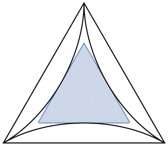
(a) $\left(\dfrac{\lambda_{1}}{E^{0}},\dfrac{\lambda_{2}}{E^{0}},\dfrac{\lambda_{3}}{E^{0}}\right)$ are taken as barycentric coordinates within the triangle. The outer triangle is the realizability domain. The curves correspond to the outer boundary of the constraints (50). The blue region gives non-negative ansatz for 3D $B_{2}$ model for all $\mathbf{E}^{1}$ satisfying $|F_{j}|\leq\lambda_{j}$, $j=1,2,3$.

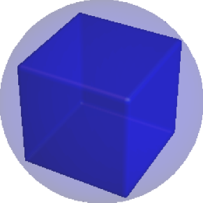
(b) The sphere correspond to the realizability domain of $\mathbf{E}^{1}$ when $\lambda_{1}=\lambda_{2}=\lambda_{3}$.The rectangle within the sphere is the region for $\mathbf{E}^{1}$ when the 3D $B_{2}$ model has a non-negative ansatz.

Figure 2: Region which correspond to a non-negative ansatz for 3D $B_{2}$ model.

Remark 4.1.

By Lemma 3.8, for $\mathbf{E}^{1}=\boldsymbol{0}$, the third-order moments given by the 3D $B_{2}$ ansatz is a zero tensor, equal to that given by $M_{2}$. For this particular case, even when there is no non-negative ansatz, the closure relation is still realizable.

We proceed to study the hyperbolicity of the model. Due to the extreme complexity of the formula, we restrict our discussions to the case that $\mathbf{E}^{1}=\boldsymbol{0}$. We first prove the following facts:

Lemma 4.1.

In the interior of the realizability domain $\mathcal{M}$, if $\mathbf{E}^{1}=\boldsymbol{0}$, we have

$$w_{i}>0,\quad\sigma_{i}+w_{i}>0,\quad i=1,2,3.$$

Proof.

Take $i=1$ for example. First, note

$$g(x,y;0,0)=\dfrac{2q(x,y;0,0)(x+y-1-r(x,y;0,0))}{3(x+y)^{2}}=\dfrac{2xy}{3(x+y)}.$$

Therefore,

$$\begin{split}w_{1}=&\lambda_{1}-g(\lambda_{1},\lambda_{2};0,0)-g(\lambda_{1},\lambda_{3};0,0)+2g(\lambda_{2},\lambda_{3};0,0)\\ =&\dfrac{1}{3}\left(3\lambda_{1}-\dfrac{2\lambda_{1}\lambda_{2}}{\lambda_{1}+\lambda_{2}}-\dfrac{2\lambda_{1}\lambda_{3}}{\lambda_{1}+\lambda_{3}}+\dfrac{4\lambda_{2}\lambda_{3}}{\lambda_{2}+\lambda_{3}}\right)\\ =&\dfrac{1}{3}\left(\lambda_{1}-\dfrac{2\lambda_{1}\lambda_{2}}{\lambda_{1}+\lambda_{2}}+2\lambda_{1}-\dfrac{2\lambda_{1}\lambda_{3}}{\lambda_{1}+\lambda_{3}}+\dfrac{4\lambda_{2}\lambda_{3}}{\lambda_{2}+\lambda_{3}}\right)\\ =&\dfrac{1}{3}\left(\lambda_{1}-\dfrac{2\lambda_{1}\lambda_{2}}{\lambda_{1}+\lambda_{2}}+\dfrac{2\lambda_{1}(\lambda_{1}+\lambda_{3}-\lambda_{3})}{\lambda_{1}+\lambda_{3}}+\dfrac{4\lambda_{2}\lambda_{3}}{\lambda_{2}+\lambda_{3}}\right)\\ =&\dfrac{1}{3}\left(\lambda_{1}-\dfrac{2\lambda_{1}\lambda_{2}}{\lambda_{1}+\lambda_{2}}+\dfrac{2\lambda_{1}^{2}}{\lambda_{1}+\lambda_{3}}+\dfrac{4\lambda_{2}\lambda_{3}}{\lambda_{2}+\lambda_{3}}\right).\end{split}$$

We need to prove $w_{1}\geq 0$ for two cases:

1. $\lambda_{1}\geq\lambda_{2}$ or $\lambda_{1}\geq\lambda_{3}$. Because $w_{1}$ is symmetric with respect to $\lambda_{2}$ and $\lambda_{3}$, we only need to discuss the case $\lambda_{1}\geq\lambda_{2}$.

2. $\lambda_{1}<\lambda_{2}$ and $\lambda_{1}<\lambda_{3}$. Due to $w_{1}$ being symmetric about $\lambda_{2}$ and $\lambda_{3}$, we only need to discuss the case $\lambda_{1}<\lambda_{2}\leq\lambda_{3}$.

The proof is as follows:

1. If $\lambda_{1}\geq\lambda_{2}$, then

   $$-\dfrac{2\lambda_{1}\lambda_{2}}{\lambda_{1}+\lambda_{2}}\geq-\dfrac{2\lambda_{1}\lambda_{2}}{\lambda_{2}+\lambda_{2}}=-\lambda_{1},$$

   therefore

   $$w_{1}=\dfrac{1}{3}\left(\lambda_{1}-\dfrac{2\lambda_{1}\lambda_{2}}{\lambda_{1}+\lambda_{2}}+\dfrac{2\lambda_{1}^{2}}{\lambda_{1}+\lambda_{3}}+\dfrac{4\lambda_{2}\lambda_{3}}{\lambda_{2}+\lambda_{3}}\right)\geq\dfrac{1}{3}\left(\dfrac{2\lambda_{1}^{2}}{\lambda_{1}+\lambda_{3}}+\dfrac{4\lambda_{2}\lambda_{3}}{\lambda_{2}+\lambda_{3}}\right)>0.$$

2. If $\lambda_{1}<\lambda_{2}\leq\lambda_{3}$, then

   $$-\dfrac{2\lambda_{1}\lambda_{2}}{\lambda_{1}+\lambda_{2}}\geq-\dfrac{2\lambda_{1}\lambda_{2}}{\lambda_{1}+\lambda_{1}}=-\lambda_{2},$$

   and

   $$\dfrac{4\lambda_{2}\lambda_{3}}{\lambda_{2}+\lambda_{3}}\geq\dfrac{4\lambda_{2}\lambda_{3}}{\lambda_{3}+\lambda_{3}}=2\lambda_{2}.$$

   Therefore

   $$w_{1}=\dfrac{1}{3}\left(\lambda_{1}-\dfrac{2\lambda_{1}\lambda_{2}}{\lambda_{1}+\lambda_{2}}+\dfrac{2\lambda_{1}^{2}}{\lambda_{1}+\lambda_{3}}+\dfrac{4\lambda_{2}\lambda_{3}}{\lambda_{2}+\lambda_{3}}\right)\geq\dfrac{1}{3}\left(\lambda_{1}-\lambda_{2}+\dfrac{2\lambda_{1}^{2}}{\lambda_{1}+\lambda_{3}}+2\lambda_{2}\right)>0.$$

This proves $w_{1}>0$. Similarly, $w_{j}>0$, $j=2,3$.

Next, we prove $\sigma_{1}+w_{1}>0$. We have

$$\sigma_{1}+w_{1}=\dfrac{2}{3}\left(3\lambda_{1}-\dfrac{2\lambda_{1}\lambda_{2}}{\lambda_{1}+\lambda_{2}}-\dfrac{2\lambda_{1}\lambda_{3}}{\lambda_{1}+\lambda_{3}}+\dfrac{2\lambda_{2}\lambda_{3}}{\lambda_{2}+\lambda_{3}}\right)=\dfrac{2}{3}\left(\lambda_{1}-\dfrac{2\lambda_{1}\lambda_{2}}{\lambda_{1}+\lambda_{2}}+\dfrac{2\lambda_{1}^{2}}{\lambda_{1}+\lambda_{3}}+\dfrac{2\lambda_{2}\lambda_{3}}{\lambda_{2}+\lambda_{3}}\right).$$

Similar to discussions on $w_{1}$, we have

1. If $\lambda_{1}\geq\lambda_{2}$, then

   $$\sigma_{1}+w_{1}=\dfrac{2}{3}\left(\lambda_{1}-\dfrac{2\lambda_{1}\lambda_{2}}{\lambda_{1}+\lambda_{2}}+\dfrac{2\lambda_{1}^{2}}{\lambda_{1}+\lambda_{3}}+\dfrac{2\lambda_{2}\lambda_{3}}{\lambda_{2}+\lambda_{3}}\right)\geq\dfrac{2}{3}\left(\dfrac{2\lambda_{1}^{2}}{\lambda_{1}+\lambda_{3}}+\dfrac{2\lambda_{2}\lambda_{3}}{\lambda_{2}+\lambda_{3}}\right).$$

2. If $\lambda_{1}<\lambda_{2}\leq\lambda_{3}$, then

   $$\sigma_{1}+w_{1}=\dfrac{2}{3}\left(\lambda_{1}-\dfrac{2\lambda_{1}\lambda_{2}}{\lambda_{1}+\lambda_{2}}+\dfrac{2\lambda_{1}^{2}}{\lambda_{1}+\lambda_{3}}+\dfrac{2\lambda_{2}\lambda_{3}}{\lambda_{2}+\lambda_{3}}\right)\geq\dfrac{2}{3}\left(\lambda_{1}-\lambda_{2}+\dfrac{2\lambda_{1}^{2}}{\lambda_{1}+\lambda_{3}}+\lambda_{2}\right)>0.$$

Similarly, $\sigma_{i}+w_{i}>0$, $i=2,3$. ∎

To study hyperbolicity, we start with calculating the Jacobian matrix of the flux $\mathbf{f}_{x}$, $\mathbf{f}_{y}$, and $\mathbf{f}_{z}$. Due to the rotational invariance of the 3D $B_{2}$ model, it could be assumed without loss of generality that $\boldsymbol{\mathit{E}}^{2}$ is diagonal, $\mathbf{R}_{1}$ is parallel to the $x$-axis, $\mathbf{R}_{2}$ is parallel to the $y$-axis, and $\mathbf{R}_{3}$ is parallel to the $z$-axis, respectively. The most involving part in calculating the Jacobian matrix is the derivatives of third-order moments. We first note that, by Lemma 3.8, fixing $\mathbf{E}^{1}=\boldsymbol{0}$ makes the value of all third-order moments zero, no matter what the values of the other moments are. Therefore,

$$\dfrac{\partial E^{3}_{ijk}}{\partial E^{0}}=0,\quad\dfrac{\partial E^{3}_{ijk}}{\partial E^{2}_{lm}}=0,\quad\forall i,j,k,l,m=1,2,3.$$

So we only need to compute $\dfrac{\partial E^{3}_{ijk}}{\partial E^{1}_{l}}$. First, we have

$$\begin{split}\dfrac{\partial E^{3}_{123}}{\partial E^{1}_{l}}=&\dfrac{\partial\left\langle(\boldsymbol{\Omega}\cdot\mathbf{R}_{i})(\boldsymbol{\Omega}\cdot\mathbf{R}_{j})(\boldsymbol{\Omega}\cdot\mathbf{R}_{k})\hat{I}_{B}\right\rangle}{\partial E^{1}_{l}}R_{i1}R_{j2}R_{k3}\\ =&\dfrac{\partial\left\langle(\boldsymbol{\Omega}\cdot\mathbf{R}_{1})(\boldsymbol{\Omega}\cdot\mathbf{R}_{2})(\boldsymbol{\Omega}\cdot\mathbf{R}_{3})\hat{I}_{B}\right\rangle}{\partial E^{1}_{l}}=0.\end{split}$$

For the terms $\dfrac{\partial E^{3}_{iij}}{\partial E^{1}_{k}}$, we have

$$\dfrac{\partial E^{3}_{iij}}{\partial E^{1}_{k}}=\dfrac{\partial\left\langle(\boldsymbol{\Omega}\cdot\mathbf{R}_{l})(\boldsymbol{\Omega}\cdot\mathbf{R}_{m})(\boldsymbol{\Omega}\cdot\mathbf{R}_{n})\hat{I}_{B}\right\rangle}{\partial E^{1}_{k}}R_{li}R_{mi}R_{nj}=\dfrac{\partial\left\langle(\boldsymbol{\Omega}\cdot\mathbf{R}_{i})^{2}(\boldsymbol{\Omega}\cdot\mathbf{R}_{j})\hat{I}_{B}\right\rangle}{\partial E^{1}_{k}}.$$

And by

$$F_{i}=\mathbf{E}^{1}\cdot\mathbf{R}_{i}=E^{1}_{1}R_{1i}+E^{1}_{2}R_{2i}+E^{1}_{3}R_{3i},$$

we get $\dfrac{\partial F_{i}}{\partial E^{1}_{k}}=\delta_{ik}$, which is used below in computing $\dfrac{\partial E^{3}_{iij}}{\partial E^{1}_{k}}$.

If $i=j$ and $k\mathrel{\mathchoice{\ooalign{$\hfil\displaystyle/\hfil$\crcr$\displaystyle=$}}{\ooalign{$\hfil\textstyle/\hfil$\crcr$\textstyle=$}}{\ooalign{$\hfil\scriptstyle/\hfil$\crcr$\scriptstyle=$}}{\ooalign{$\hfil\scriptscriptstyle/\hfil$\crcr$\scriptscriptstyle=$}}}i$,

$$\dfrac{\partial\left\langle(\boldsymbol{\Omega}\cdot\mathbf{R}_{i})^{3}\hat{I}_{B}\right\rangle}{\partial E^{1}_{k}}=F_{i}\dfrac{\partial}{\partial E^{1}_{k}}\left(\dfrac{\sigma_{i}^{2}+2F_{i}^{2}-3w_{i}\sigma_{i}}{2F_{i}^{2}-w_{i}\sigma_{i}-w_{i}^{2}}\right)=0.$$

And if $i\mathrel{\mathchoice{\ooalign{$\hfil\displaystyle/\hfil$\crcr$\displaystyle=$}}{\ooalign{$\hfil\textstyle/\hfil$\crcr$\textstyle=$}}{\ooalign{$\hfil\scriptstyle/\hfil$\crcr$\scriptstyle=$}}{\ooalign{$\hfil\scriptscriptstyle/\hfil$\crcr$\scriptscriptstyle=$}}}j$ and $k\mathrel{\mathchoice{\ooalign{$\hfil\displaystyle/\hfil$\crcr$\displaystyle=$}}{\ooalign{$\hfil\textstyle/\hfil$\crcr$\textstyle=$}}{\ooalign{$\hfil\scriptstyle/\hfil$\crcr$\scriptstyle=$}}{\ooalign{$\hfil\scriptscriptstyle/\hfil$\crcr$\scriptscriptstyle=$}}}j$,

$$\dfrac{\partial\left\langle(\boldsymbol{\Omega}\cdot\mathbf{R}_{i})^{2}(\boldsymbol{\Omega}\cdot\mathbf{R}_{j})\hat{I}_{B}\right\rangle}{\partial E^{1}_{k}}=\dfrac{F_{j}}{2}\dfrac{\partial}{\partial E^{1}_{k}}\left(1-\dfrac{\sigma_{j}^{2}+2F_{j}^{2}-3w_{j}\sigma_{j}}{2F_{j}^{2}-w_{j}\sigma_{j}-w_{j}^{2}}\right)=0.$$

Therefore, the non-zero entries in the Jacobian matrix can be $\dfrac{\partial E^{3}_{iij}}{\partial E^{1}_{j}}$ only. By rotational invariance of the model, we need only study the Jacobian matrix in the $x$-direction, $\dfrac{\partial\mathbf{f}_{x}}{\partial\mathbf{E}}$, which is

$$\boldsymbol{\mathrm{J}}_{x}=\left(\begin{array}[]{ccccccccc}0&1&0&0&0&0&0&0&0\\ 0&0&0&0&1&0&0&0&0\\ 0&0&0&0&0&1&0&0&0\\ 0&0&0&0&0&0&1&0&0\\ 0&\dfrac{\partial E^{3}_{111}}{\partial E^{1}_{1}}&0&0&0&0&0&0&0\\ 0&0&\dfrac{\partial E^{3}_{112}}{\partial E^{1}_{2}}&0&0&0&0&0&0\\ 0&0&0&\dfrac{\partial E^{3}_{113}}{\partial E^{1}_{3}}&0&0&0&0&0\\ 0&\dfrac{\partial E^{3}_{122}}{\partial E^{1}_{1}}&0&0&0&0&0&0&0\\ 0&0&0&0&0&0&0&0&0\end{array}\right).$$ (52)

For the non-zero entries in $\boldsymbol{\mathrm{J}}_{x}$, we have the following bounds:

Lemma 4.2.

In the interior of the realizability domain $\mathcal{M}$, if $\mathbf{E}^{1}=\boldsymbol{0}$, we have

1. $0<\dfrac{\partial E^{3}_{11k}}{\partial E^{1}_{k}}<\dfrac{1}{2}$, for $k=2,3$;

2. $0<\dfrac{\partial E^{3}_{111}}{\partial E^{1}_{1}}\leq 1$ if and only if $\sigma_{1}>0$.

Proof.

For the first item, we only need to verify for $k=2$. By Lemma 3.8, one has

$$\begin{split}\dfrac{\partial E^{3}_{112}}{\partial E^{1}_{2}}=&\dfrac{\partial\left\langle(\boldsymbol{\Omega}\cdot\mathbf{R}_{1})^{2}(\boldsymbol{\Omega}\cdot\mathbf{R}_{2})\hat{I}_{B}\right\rangle}{\partial E^{1}_{2}}\\ =&\dfrac{1}{2}\left(1-\dfrac{\sigma_{2}^{2}+2F_{2}^{2}-3w_{2}\sigma_{2}}{2F_{2}^{2}-w_{2}\sigma_{2}-w_{2}^{2}}\right)\\ =&\dfrac{1}{2}\dfrac{(w_{2}-\sigma_{2})^{2}}{w_{2}(\sigma_{2}+w_{2})}.\end{split}$$

By Lemma 4.1 we have $w_{2}>0$ and $\sigma_{2}+w_{2}>0$, thus, $\dfrac{\partial E^{3}_{112}}{\partial E^{1}_{2}}>0$. In addition, from the proof of Theorem 4.2, we have $\sigma_{2}\leq w_{2}$, therefore $\dfrac{\partial E^{3}_{112}}{\partial E^{1}_{2}}<\dfrac{1}{2}$.

For the second item, we have by Lemma 3.8,

$$\dfrac{\partial E^{3}_{111}}{\partial E^{1}_{1}}= \dfrac{\partial\left\langle(\boldsymbol{\Omega}\cdot\mathbf{R}_{1})^{3}\hat{I}_{B}\right\rangle}{\partial E^{1}_{1}}=\dfrac{\sigma_{1}^{2}+2F_{1}^{2}-3w_{1}\sigma_{1}}{2F_{1}^{2}-w_{1}\sigma_{1}-w_{1}^{2}}$$

$$= \dfrac{\sigma_{1}(3w_{1}-\sigma_{1})}{w_{1}(\sigma_{1}+w_{1})}=1-\dfrac{(w_{1}-\sigma_{1})^{2}}{w_{1}(\sigma_{1}+w_{1})}\leq 1,$$

And $\dfrac{\partial E^{3}_{111}}{\partial E^{1}_{1}}>0$ is equivalent to $\sigma_{1}(3w_{1}-\sigma_{1})>0$. As $\sigma_{1}\leq w_{1}$, we have $3w_{1}-\sigma_{1}\geq 2w_{1}>0$, implying that $\dfrac{\partial E^{3}_{111}}{\partial E^{1}_{1}}>0$ is equivalent to $\sigma_{1}>0$. ∎

We now give the condition for the real diagonalizability of the Jacobian matrix $\boldsymbol{\mathrm{J}}_{x}$ as follows:

Theorem 4.3.

The Jacobian matrix $\boldsymbol{\mathrm{J}}_{x}$ defined in (52) is real diagonalizable if and only if $\sigma_{1}>0$.

Proof.

The characteristic polynomial of $\boldsymbol{\mathrm{J}}_{x}$ is

$$\left|\lambda\mathbf{I}-\boldsymbol{\mathrm{J}}_{x}\right|=\lambda^{3}\left(\lambda^{2}-\dfrac{\partial E^{3}_{111}}{\partial E^{1}_{1}}\right)\left(\lambda^{2}-\dfrac{\partial E^{3}_{112}}{\partial E^{1}_{2}}\right)\left(\lambda^{2}-\dfrac{\partial E^{3}_{113}}{\partial E^{1}_{3}}\right),$$ (53)

thus zero is a multiple eigenvalue of $\boldsymbol{\mathrm{J}}_{x}$. The corresponding eigenvectors are

$$(0,0,0,0,0,0,0,0,1)^{T},\quad(0,0,0,0,0,0,0,1,0)^{T},\quad(1,0,0,0,0,0,0,0,0)^{T}.$$

In the case that

$$\dfrac{\partial E^{3}_{111}}{\partial E^{1}_{1}}\geq 0,\quad\dfrac{\partial E^{3}_{112}}{\partial E^{1}_{2}}\geq 0,\quad\dfrac{\partial E^{3}_{113}}{\partial E^{1}_{3}}\geq 0,$$

the corresponding eigenvalues of the matrix are

$$\lambda_{1}=\pm\sqrt{\dfrac{\partial E^{3}_{111}}{\partial E^{1}_{1}}},\quad\lambda_{2}=\pm\sqrt{\dfrac{\partial E^{3}_{112}}{\partial E^{1}_{2}}},\quad\lambda_{3}=\pm\sqrt{\dfrac{\partial E^{3}_{113}}{\partial E^{1}_{3}}},\quad$$

and the corresponding eigenvectors are

$$\begin{array}[]{cccccc}\left(\begin{array}[]{c}1\\ \lambda_{1}\\ 0\\ 0\\ |\lambda_{1}|^{2}\\ 0\\ 0\\ \dfrac{\partial E^{3}_{122}}{\partial E^{1}_{1}}\\ 0\end{array}\right),\qquad\left(\begin{array}[]{c}0\\ 0\\ -1\\ 0\\ 0\\ \lambda_{2}\\ 0\\ 0\\ 0\end{array}\right),\qquad\left(\begin{array}[]{c}0\\ 0\\ 0\\ -1\\ 0\\ 0\\ \lambda_{3}\\ 0\\ 0\end{array}\right).\end{array}$$

It could be verified directly that if any of the eigenvalues $\lambda_{i}$, $i=1,2,3$, equals zero, the Jacobian matrix is not real diagonalizable. If we have

$$\dfrac{\partial E^{3}_{111}}{\partial E^{1}_{1}}>0,\quad\dfrac{\partial E^{3}_{112}}{\partial E^{1}_{2}}>0,\quad\dfrac{\partial E^{3}_{113}}{\partial E^{1}_{3}}>0,$$ (54)

by the linear independence of the eigenvectors, one concludes that the Jacobian matrix is real diagonalizable. Then the proof is finished by Lemma 4.2. ∎

As a direct consequence of Theorem 4.3, the 3D $B_{2}$ model is hyperbolic at equilibrium. This can be proved by the following arguments. Let $\mathbf{R}_{j}$, $j=1,2,3$ be the three eigenvectors of $\boldsymbol{\mathit{E}}^{2}$. Denote the $k$-th component of the vector $\mathbf{R}_{j}$ to be $R_{kj}$. Define the Jacobian matrix of the 3D $B_{2}$ model (13) along $\mathbf{R}_{j}$, $j=1,2,3$ to be $\tsum\slimits@\limits_{k=1}^{3}R_{kj}\mathbf{J}_{k}$. Theorem 4.3 shows that for the cases $\mathbf{E}^{1}=\boldsymbol{0}$, condition (50) is the necessary and sufficient condition for the Jacobian matrix along $\mathbf{R}_{j}$, $\forall j=1,2,3$ to be real diagonalizable. The above result holds because for any given $\mathbf{R}_{j}$, $j=1,2,3$, we could always rotate the coordinate system, such that $\mathbf{R}_{j}$ is aligned with the $x$-axis. Theorem 4.2 gives (51) as the necessary and sufficient condition for $\sigma_{1}>0$, and rotation of coordinates can permute the indices in (51), which results in (50). Notice that at equilibrium, $\boldsymbol{\mathit{E}}^{2}$ is a scalar matrix, so any direction is an eigenvector of $\boldsymbol{\mathit{E}}^{2}$. Therefore, the 3D $B_{2}$ model is hyperbolic at equilibrium.

For given moments, we could always choose a coordinate system such that $\boldsymbol{\mathit{E}}^{2}$ is a diagonal matrix. The system is hyperbolic if and only if for an arbitrary $\mathbf{n}\mathrel{\mathchoice{\ooalign{$\hfil\displaystyle/\hfil$\crcr$\displaystyle=$}}{\ooalign{$\hfil\textstyle/\hfil$\crcr$\textstyle=$}}{\ooalign{$\hfil\scriptstyle/\hfil$\crcr$\scriptstyle=$}}{\ooalign{$\hfil\scriptscriptstyle/\hfil$\crcr$\scriptscriptstyle=$}}}\boldsymbol{0}$, we always have $n_{x}\mathbf{J}_{x}+n_{y}\mathbf{J}_{y}+n_{z}\mathbf{J}_{z}$ to be real diagonalizable. For $\mathbf{E}^{1}=\boldsymbol{0}$, we sample for all possible $(\lambda_{1},\lambda_{2},\lambda_{3})$ and all unit vectors $\mathbf{n}$, to check if the matrix is real diagonalizable. There is a hyperbolicity region around equilibrium for $\mathbf{E}^{1}=\boldsymbol{0}$ as in Figure 3. The hyperbolicity region is a smaller region than that enclosed by (50). However, it does cover a neighborhood of the equilibrium.

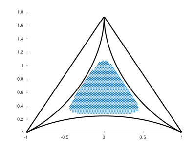
Figure 3: Region of hyperbolicity when $\mathbf{E}^{1}=\boldsymbol{0}$. $\left(\dfrac{\lambda_{1}}{E^{0}},\dfrac{\lambda_{2}}{E^{0}},\dfrac{\lambda_{3}}{E^{0}}\right)$ are taken as barycentric coordinates within the triangle. The outer triangle is the realizability domain. The curves correspond to the outer boundary of the constraints (50). The 3D $B_{2}$ model is found to be hyperbolic within the dotted blue region.

Finally, we point out that although the 3D $B_{2}$ model is aimed at approximating the $M_{2}$ model, there is an interesting difference between them. This difference arises from the fact that the ansatz is assumed to be the form $\hat{I}_{B}$ in (12), and is independent of choice for the function $f(\mu;\gamma,\delta)$. When the given moments satisfy

$$\exists i\mathrel{\mathchoice{\ooalign{$\hfil\displaystyle/\hfil$\crcr$\displaystyle=$}}{\ooalign{$\hfil\textstyle/\hfil$\crcr$\textstyle=$}}{\ooalign{$\hfil\scriptstyle/\hfil$\crcr$\scriptstyle=$}}{\ooalign{$\hfil\scriptscriptstyle/\hfil$\crcr$\scriptscriptstyle=$}}}j,\text{ such that }\lambda_{i}=\lambda_{j},~{}~{}\text{and}~{}~{}F_{i}=F_{j}=0,$$ (55)

the corresponding ansatz in the $M_{2}$ model is an axisymmetric function. This includes the equilibrium distribution. Exactly at the equilibrium, the 3D $B_{2}$ ansatz $\hat{I}_{B}$ is isotropic, and, thus, axisymmetric. However, even in neighbourhoods of the equilibrium, moments corresponding to an axisymmetric ansatz in the $M_{2}$ model would usually not reproduce an axisymmetric ansatz for the 3D $B_{2}$ model. In other words, for arbitrary $\epsilon>0$, there exist moments in the set

$$\mathcal{A}_{\epsilon}=\left\{(E^{0},\mathbf{E}^{1},\boldsymbol{\mathit{E}}^{2})\in\mathcal{M}~{}\Big{|}~{}\mathbf{E}^{1}=\boldsymbol{0},\tsum\slimits@_{i=1}^{3}\left|\lambda_{i}-\dfrac{E^{0}}{3}\right|^{2}<\epsilon,\text{ and \eqref{eq:moments-with-axisymmetric-M2-ansatz} is valid}\right\},$$

for which the 3D $B_{2}$ ansatz $\hat{I}_{B}$ is not axisymmetric; otherwise, the closure relation may lose the necessary regularities. More precisely, we claim:

Theorem 4.4.

There are no functions $w_{i}(\lambda_{1},\lambda_{2},\lambda_{3};F_{1},F_{2},F_{3})$, $i=1,2,3$, in the 3D $B_{2}$ ansatz $\hat{I}_{B}$ satisfying both items below:

1. $w_{i}$, $i=1,2,3$, are differentiable at the equilibrium state.

2. The ansatz $\hat{I}_{B}$ is axisymmetric for any moments in $\mathcal{A}_{\epsilon}$.

Proof.

We prove by contradiction. Suppose that (12) is an axisymmetric distribution. Without losing generality we assume the corresponding moments satisfy $\lambda_{2}=\lambda_{3}$, therefore the symmetric axis is aligned to $\mathbf{R}_{1}$, and $F_{2}=F_{3}=0$. To get axisymmetry in (12), the contributions from $w_{2}f(\boldsymbol{\Omega}\cdot\mathbf{R}_{2};\gamma_{2},\delta_{2})$ and $w_{3}f(\boldsymbol{\Omega}\cdot\mathbf{R}_{3};\gamma_{3},\delta_{3})$ have to be either zero or constant functions, hence $\sigma_{2}=\dfrac{w_{2}}{3}$ and $\sigma_{3}=\dfrac{w_{3}}{3}$, giving

$$\sigma_{1}+\sigma_{2}+\sigma_{3}=\lambda_{1}.$$

Similar relations could be obtained when the symmetric axis is aligned to $\mathbf{R}_{2}$ or $\mathbf{R}_{3}$. Consider the case when $\mathbf{E}^{1}=\boldsymbol{0}$. Let

$$\sigma(\lambda_{1},\lambda_{2},\lambda_{3})=\sigma_{1}(\lambda_{1},\lambda_{2},\lambda_{3};0,0,0)+\sigma_{2}(\lambda_{1},\lambda_{2},\lambda_{3};0,0,0)+\sigma_{3}(\lambda_{1},\lambda_{2},\lambda_{3};0,0,0).$$

Based on the above arguments, we have

$$\sigma(\lambda_{1},\lambda_{2},\lambda_{3})=\left\{\begin{array}[]{l}\lambda_{1},\quad\text{if}\quad\lambda_{2}=\lambda_{3}=\frac{1}{2}(E^{0}-\lambda_{1}),\\ \lambda_{2},\quad\text{if}\quad\lambda_{1}=\lambda_{3}=\frac{1}{2}(E^{0}-\lambda_{2}),\\ \lambda_{3},\quad\text{if}\quad\lambda_{1}=\lambda_{2}=\frac{1}{2}(E^{0}-\lambda_{3}).\end{array}\right.$$ (56)

If all $w_{i}$, $i=1,2,3$, are differentiable, then all $\sigma_{i}$, $i=1,2,3$, are differentiable, so $\nabla\sigma$ should be a continuous function for all realizabile moments. Let

$$\mathbf{n}_{1}=(1,-\frac{1}{2},-\frac{1}{2}),\quad\mathbf{n}_{2}=(-\frac{1}{2},1,-\frac{1}{2}),\quad\mathbf{n}_{3}=(-\frac{1}{2},-\frac{1}{2},1),$$

then $\nabla\sigma\cdot(\mathbf{n}_{1}+\mathbf{n}_{2}+\mathbf{n}_{3})=0$. On the other hand, $\nabla\sigma\cdot\mathbf{n}_{1}$ is equivalent to taking the derivative of $\sigma$ along $\lambda_{2}=\lambda_{3}=\frac{1}{2}(E^{0}-\lambda_{1})$, and we have similar relationships for $\mathbf{n}_{2}$ and $\mathbf{n}_{3}$. So evaluating $\nabla\sigma\cdot\mathbf{n}_{j}$ at $\lambda_{j}=\dfrac{E^{0}}{3}$, $j=1,2,3$ and $\mathbf{E}^{1}=\boldsymbol{0}$ according to (56) gives $\nabla\sigma\cdot(\mathbf{n}_{1}+\mathbf{n}_{2}+\mathbf{n}_{3})=3$, leading to a contradiction. Therefore the two items can not be satisfied simultaneously. ∎

Notice that the proof of this lemma does not make use of the specific form of the function $f$ in (12). In fact, it can be seen from the proof that this inconsistency is due to the fact that the ansatz is a linear combination of three axisymmetric distributions. However, although the new model does not reproduce an axisymmetric ansatz for moments corresponding to an axisymmetric ansatz in the $M_{2}$ model, in such cases the closure of the new model retain the same structure as the $M_{2}$ closure. Without loss of generality consider the case when $\lambda_{2}=\lambda_{3}=0$ and $F_{2}=F_{3}=0$. From (38), we have

$$\begin{split}&\left\langle(\boldsymbol{\Omega}\cdot\mathbf{R}_{1})^{2}(\boldsymbol{\Omega}\cdot\mathbf{R}_{2})\hat{I}_{B}\right\rangle=\left\langle(\boldsymbol{\Omega}\cdot\mathbf{R}_{1})^{2}(\boldsymbol{\Omega}\cdot\mathbf{R}_{3})\hat{I}_{B}\right\rangle=0,\\ &\left\langle(\boldsymbol{\Omega}\cdot\mathbf{R}_{1})(\boldsymbol{\Omega}\cdot\mathbf{R}_{2})^{2}\hat{I}_{B}\right\rangle=\left\langle(\boldsymbol{\Omega}\cdot\mathbf{R}_{3})(\boldsymbol{\Omega}\cdot\mathbf{R}_{2})^{2}\hat{I}_{B}\right\rangle=\dfrac{1}{2}\left(F_{1}-\left\langle(\boldsymbol{\Omega}\cdot\mathbf{R}_{1})^{3}\right\rangle\right),\end{split}$$ (57)

satisfying the same equalities as that given by an $M_{2}$ ansatz with $\mathbf{R}_{1}$ as the symmetric axis.

Define

$$E_{1}=\dfrac{\|\mathbf{E}^{1}\|}{E^{0}},\quad E_{2}=\dfrac{1}{(E^{0})^{3}}(\mathbf{E}^{1})^{T}\boldsymbol{\mathit{E}}^{2}\mathbf{E}^{1},\quad E_{3}=\dfrac{1}{(E^{0})^{4}}\left\langle\left(\boldsymbol{\Omega}\cdot\mathbf{E}^{1}\right)^{3}\hat{I}\right\rangle.$$

Then $E_{i}$, $i=1,2,3$ would be the scaled first, second and third-order moments for slab geometry cases. We compare the contour of $E_{3}$ between the 3D $B_{2}$ model and the $M_{2}$ model for slab geometry in Figure 4. It is shown in Figure 4 that the 3D $B_{2}$ model provides realizable closure which is qualitatively similar to that of $M_{2}$ closure for most of realizable moments.

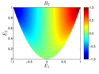
(a) The value of $E_{3}$ in slab geometry for normalized realizable moments using the 3D $B_{2}$ closure.

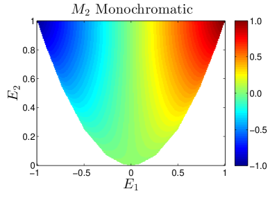
(b) The value of $E_{3}$ for normalized realizable moments using the maximum entropy closure in slab geometry for the monochromatic case.

Figure 4: Comparing the value of the closing moment $E_{3}$ for $M_{2}$ for the monochromatic case and for the 3D $B_{2}$ model in slab geometry.

5 Conclusion and Future Work

We proposed a 3D $B_{2}$ model that is an extension of the EQMOM ($B_{2}$ model) in 1D. We showed, step by step, how the structure of the new model is gradually refined. Particularly, we studied the main properties of this new model, including rotational invariance, realizability, and hyperbolicity.

We are currently carrying out numerical simulations using the new model. For the first step, we hope that the model provides satisfactory results on standard benchmark problems.

References

[1]
Graham W Alldredge, Cory D Hauck, Dianne P OʼLeary, and André L Tits.
Adaptive change of basis in entropy-based moment closures for linear
kinetic equations.
Journal of Computational Physics, 258:489–508, 2014.
[2]
Graham W Alldredge, Cory D Hauck, and André L Tits.
High-order entropy-based closures for linear transport in slab
geometry ii: A computational study of the optimization problem.
SIAM Journal on Scientific Computing, 34(4):B361–B391, 2012.
[3]
Graham W Alldredge, Ruo Li, and Weiming Li.
Approximating the m 2 method by the extended quadrature method of
moments for radiative transfer in slab geometry.
Kinetic & Related Models, 9(2), 2016.
[4]
R. Curto and L. Fialkow.
Recursiveness, positivity and truncated moment problems.
Houston J. Math, 17(4):603–635, 1991.
[5]
B. Dubroca and J.-L. Fuegas.
Étude théorique et numérique d’une hiérarchie de modèles
aus moments pour le transfert radiatif.
C.R. Acad. Sci. Paris, I. 329:915–920, 1999.
[6]
Martin Frank, Bruno Dubroca, and Axel Klar.
Partial moment entropy approximation to radiative heat transfer.
Journal of Computational Physics, 218(1):1–18, 2006.
[7]
C Kristopher Garrett, Cory Hauck, and Judith Hill.
Optimization and large scale computation of an entropy-based moment
closure.
Journal of Computational Physics, 2015.
[8]
Norman Lloyd Johnson and Samuel Kotz.
Discrete Distributions: Continuous Univariate Distributions-2.
Wiley, 1970.
[9]
Michael Junk.
Maximum entropy for reduced moment problems.
Mathematical Models and Methods in Applied Sciences,
10(07):1001–1025, 2000.
[10]
DS Kershaw.
Flux limiting nature’s own way.
Lawrence Livermore National Laboratory, UCRL-78378, 1976.
[11]
C David Levermore.
Moment closure hierarchies for kinetic theories.
Journal of Statistical Physics, 83(5-6):1021–1065, 1996.
[12]
E. E. Lewis and W. F. Miller, Jr.
Computational Methods in Neutron Transport.
John Wiley and Sons, New York, 1984.
[13]
T Pichard, GW Alldredge, S Brull, B Dubroca, and M Frank.
An approximation of the m_2 closure: Application to radiotherapy
dose simulation.
Journal of Scientific Computing, pages 1–38, 2016.
[14]
Gerald C Pomraning.
The equations of radiation hydrodynamics.
Courier Dover Publications, 1973.
[15]
Florian Schneider.
Kershaw closures for linear transport equations in slab geometry i:
Model derivation.
Journal of Computational Physics, 322:905 – 919, 2016.
[16]
V Vikas, CD Hauck, ZJ Wang, and Rodney O Fox.
Radiation transport modeling using extended quadrature method of
moments.
Journal of Computational Physics, 246:221–241, 2013.
[17]
Kai-Bor Yu.
Recursive updating the eigenvalue decomposition of a covariance
matrix.
Signal Processing, IEEE Transactions on, 39(5):1136–1145,
1991.