The multidegree of the multi-image variety

Abstract

The multi-image variety is a subvariety of $\operatorname{Gr}(1,\mathbb{P}^{3})^{n}$ that models taking pictures with $n$ rational cameras. We compute its cohomology class in the cohomology of $\operatorname{Gr}(1,\mathbb{P}^{3})^{n}$, and from there its multidegree as a subvariety of $(\mathbb{P}^{5})^{n}$ under the Plücker embedding.

1 Introduction

Multi-view geometry studies the constraints imposed on a three-dimensional scene from various two-dimensional images of the scene. Each image is produced by a camera. Algebraic vision is a recent field of mathematics in which the techniques of algebraic geometry and optimization are used to formulate and solve problems in computer vision. One of the main objects studied by this field is a multi-view variety. Roughly speaking, a multi-view variety parametrizes all the possible images that can be taken by a fixed collection of cameras. See AST ; PST ; THP for more details on multi-view varieties. See SRTGB for a survey on various camera models.

The work PST presents a new point of view to study the multi-view varieties. A photographic camera maps a point in the scene to a point in the image. PST defines a geometric camera, which maps a point in the scene not to a point, but to a viewing ray. More precisely, a photographic camera is a map $\mathbb{P}^{3}\dasharrow\mathbb{P}^{2}$ or $\mathbb{P}^{3}\dasharrow\mathbb{P}^{1}\times\mathbb{P}^{1}$, whereas a geometric camera is a map $\mathbb{P}^{3}\dasharrow\operatorname{Gr}(1,\mathbb{P}^{3})$ such that the image of each point is a line containing the point. The viewing ray corresponding to a point $p\in\mathbb{P}^{3}$ is the line in $\operatorname{Gr}(1,\mathbb{P}^{3})$ this point gets mapped to. An important assumption is that light travels along rays which means that the image of a geometric camera is two-dimensional.

We now illustrate these definitions using the example of pinhole cameras or cameræ  obscuræ, see Figure 1. As a geometric camera, a pinhole camera maps a point $p\in\mathbb{P}^{3}$ to the line $\phi(p)$ connecting $p$ to the focal point. This map is rational since it is undefined at the focal point. As a photographic camera, a pinhole camera maps a point $p\in\mathbb{P}^{3}$ to the intersection of $\phi(p)$ and the plane at the back of the camera. Notice that, as a photographic camera, there are many pinhole cameras corresponding to a given focal point. All of these cameras are equivalent up to a projective transformation. The essential part of a pinhole camera is the mapping of the scene points to viewing rays, i.e. its modeling as a geometric camera.

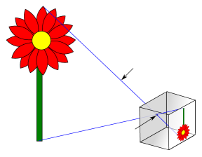
Figure 1: A pinhole camera.

A multi-image variety is the Zariski closure of the image of a map

$$\phi:\mathbb{P}^{3} \dasharrow\operatorname{Gr}(1,\mathbb{P}^{3})^{n}$$

$$p \mapsto(\phi_{1}(p),\ldots,\phi_{n}(p)),$$

where each $\phi_{i}$ is a geometric camera. The multi-view variety is a multi-image variety such that each $\phi_{i}$ is a pinhole camera. Let $C_{i}$ be the closure of the image of $\phi_{i}$ inside the $i$-th $\operatorname{Gr}(1,\mathbb{P}^{3})$. Then under some assumptions, (PST, , Theorem 5.1) shows that

$$(C_{1}\times\cdots\times C_{n})\cap V_{n}=\phi(\mathbb{P}^{3}),$$

where $V_{n}$ is the concurrent lines variety consisting of ordered $n$-tuples of lines in $\mathbb{P}^{3}$ that meet in a point $x$. The concurrent lines and multi-image varieties are embedded into $(\mathbb{P}^{5})^{n}$ using the Plücker embedding.

The multidegree of a variety embedded into a product of projective spaces is the polynomial whose coefficients give the numbers (when finite) of intersection points in the variety intersected with a product of general linear subspaces. The present paper verifies the conjectured formula (PST, , Equation (11)) for the multidegree of $V_{n}$ and computes the multidegree of the multi-image variety. To do so, we describe $V_{n}$ using a projection of a partial flag variety and use Schubert calculus to compute the cohomology classes of $V_{n}$ and $(C_{1}\times\cdots\times C_{n})\cap V_{n}$ in the cohomology ring of $\operatorname{Gr}(1,\mathbb{P}^{3})^{n}$. We then push forward these formulæ into $(\mathbb{P}^{5})^{n}$ to obtain the multidegrees.

We now describe the organization of this paper. In §2 we define the main objects of study: the multi-image variety and the concurrent lines variety. We present the main theorem which computes the multidegrees of these objects. The main tool to prove the main theorem is Schubert calculus. In §3 we give a brief introduction to Schubert calculus for $\operatorname{Gr}(1,\mathbb{P}^{3})$. In §4 we compute the cohomology class of the multi-image variety and the concurrent lines variety in terms of the Schubert cycles in $\operatorname{Gr}(1,\mathbb{P}^{3})$. We prove the main theorem by taking the pushforward of these equations to the cohomology ring of $\mathbb{P}^{5}$. In §5 we refine these results to a computation of the $K$-class for the concurrent lines variety.

2 The multi-image variety

The Grassmannian $\operatorname{Gr}(k,\mathbb{P}^{d})$ consists of $k$-dimensional planes inside $\mathbb{P}^{d}$. A congruence is a two-dimensional family of lines in $\mathbb{P}^{3}$, i.e. a surface $C$ in $\operatorname{Gr}(1,\mathbb{P}^{3})$. The bidegree $(\alpha,\beta)$ of a congruence $C$ is a pair of nonnegative integers such that the cohomology class of $C$ in $\operatorname{Gr}(1,\mathbb{P}^{3})$ has the form

$$[C]=\alpha\left[L:\ L\text{ contains a fixed point}\right]+\beta\left[L:\ L\text{ lies in a fixed plane}\right].$$ (1)

The first integer $\alpha$ is called the order and counts the number of lines in $C$ that pass through a general point of $\mathbb{P}^{3}$, and $\beta$ is called the class and counts the number of lines in $C$ that lie in a general plane of $\mathbb{P}^{3}$. The focal locus of $C$ consists of the points in $\mathbb{P}^{3}$ that do not belong to $\alpha$ distinct lines of $C$.

Example 1

A congruence with bidegree $(1,0)$ consists of all lines in $\operatorname{Gr}(1,\mathbb{P}^{3})$ that contain a fixed point. A geometric camera for such a congruence represents a pinhole camera where the fixed point is the focal point.

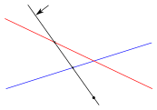
Figure 2: A two-slit camera.

Example 2

A two-slit camera assigns to $p\in\mathbb{P}^{3}$ the unique line passing through $p$ and intersecting two fixed lines $L_{1},L_{2}\in\operatorname{Gr}(1,\mathbb{P}^{3})$, see Figure 2. Its focal locus is $\{L_{1},L_{2}\}$. These cameras correspond to the congruences with bidegrees $(1,1)$.

The study of congruences started with Kum which classified those of order one. They were studied by many mathematicians during the second half of the 19th century; see the book Jes for some of these results.

Remark 1

Congruences are studied the article KNT . In particular, (KNT, , §2) discusses congruences and their bidegrees. The bidegrees of curves in $\mathbb{P}^{1}\times\mathbb{P}^{1}$ are discussed in the article NFSY .

Consider a rational map

$$\phi:\mathbb{P}^{3} \dasharrow C_{1}\times\cdots\times C_{n}\quad\subset\quad\operatorname{Gr}(1,\mathbb{P}^{3})^{n}$$

$$x \mapsto(\phi_{1}(x),\ldots,\phi_{n}(x))$$

where the closure or $\phi_{i}(\mathbb{P}^{3})$ equals $C_{i}$, each $C_{i}$ is a congruence and $x\in\phi_{i}(x)$ for all $i$. Each map $\phi_{i}$ is defined everywhere except on the focal locus of $C_{i}$. In the language of algebraic vision such a map means taking pictures with $n$ rational cameras where each $C_{i}$ is the $i$-th image plane. An important assumption is that light travels along rays which means that $C_{i}$ is $2$-dimensional.

Let $C_{1},\ldots,C_{n}$ be congruences of bidegree $(1,\beta_{i})$. Note that $\phi_{i}(x)$ is the unique line in $C_{i}$ passing through $x$. The multi-image variety of $(C_{1},\ldots,C_{n})$ is the Zariski closure of $\phi(\mathbb{P}^{3})$. The concurrent lines variety $V_{n}$ consists of ordered $n$-tuples of lines in $\mathbb{P}^{3}$ that meet in a point $x$. By (PST, , Theorem 5.1), if the focal loci of the congruences are pairwise disjoint then the multi-image equals the intersection

$$(C_{1}\times\cdots\times C_{n})\cap V_{n}\quad\subset\quad\operatorname{Gr}(1,\mathbb{P}^{3})^{n}.$$

Most of the cameras studied in computer vision are associated with congruences of order $1$. However, cameras of higher order also appear in computer vision, see SRTGB and (PST, , §7). As an example of a camera associated to a congruence of bidegree $(2,2)$ let us discuss a non-central panoramic camera, see Figure 3. Consider a circle $X$ obtained by rotating a point about a vertical axis $L$. There are two lines in $\operatorname{Gr}(1,\mathbb{P}^{3})$ passing through a general point $p\in\mathbb{P}^{3}$ and intersecting both $L$ and $X$. The congruence $C$ consisting of all lines intersecting both $X$ and $L$ has bidegree $(2,2)$. A physical realization of a non-central panoramic camera consists of a sensor on the circle taking measurements pointing outwards. This orientation of the sensor yields a map $\phi:\mathbb{P}^{3}\dasharrow\operatorname{Gr}(1,\mathbb{P}^{3})$, i.e. it assigns only one line $\phi(p)$ to a point $p\in\mathbb{P}^{3}$.

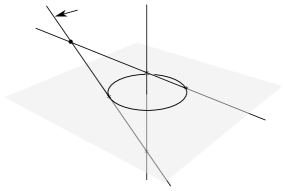
Figure 3: A non-central panoramic camera picks one of the two lines intersecting the circle $X$ and the line $L$.

The concurrent lines and multi-image varieties are embedded into $(\mathbb{P}^{5})^{n}$ using the Pücker embedding

$$\operatorname{Gr}(1,\mathbb{P}^{3})\hookrightarrow\mathbb{P}^{5}.$$

The multidegree of a variety $X$ embedded into a product of projective spaces $\mathbb{P}^{a_{1}}\times\cdots\times\mathbb{P}^{a_{n}}$ is a homogeneous polynomial whose term $q\,z_{1}^{r_{1}}\cdots z_{n}^{r_{n}}$ indicates that there are $q$ intersection points when $X$ is intersected with the product $H_{1}\times\cdots\times H_{n}\subset\mathbb{P}^{a_{1}}\times\cdots\times\mathbb{P}^{a_{n}}$ of general linear subspaces, where $\dim(H_{i})=r_{i}$. The degree of this polynomial equals the codimension of $X$ in $\mathbb{P}^{a_{1}}\times\cdots\times\mathbb{P}^{a_{n}}$. An equivalent definition of the multidegree of $X$ is its cohomology class in the cohomology ring of $\mathbb{P}^{a_{1}}\times\cdots\times\mathbb{P}^{a_{n}}$. The built-in command multidegree in the software Macaulay2 M2 computes the multidegree of $X$ from its defining ideal. We refer to the book (MS, , §8.5) for more details on multidegrees.

The main theorem of this paper computes the multidegree of the multi-image variety:

Theorem 2.1

The multidegree of the concurrent lines variety $V_{n}$ in $(\mathbb{P}^{5})^{n}$ equals

$$(z_{1}z_{2}\cdots z_{n})^{3}\left(4\sum_{(i,j)\atop i\neq j}z_{i}^{-2}z_{j}^{-1}+8\sum_{\left\{i,j,k\right\}}z_{i}^{-1}z_{j}^{-1}z_{k}^{-1}\right).$$ (2)

Let $(\alpha_{i},\beta_{i})$ be the bidegree of $C_{i}$ for $i=1,\ldots,n$. The multidegree of $(C_{1}\times\cdots\times C_{n})\cap V_{n}$ in $(\mathbb{P}^{5})^{n}$ equals

$$(\alpha_{1}\alpha_{2}\cdots\alpha_{n})(z_{1}z_{2}\cdots z_{n})^{5}\Bigg{(} \sum_{(i,j)\atop i\neq j}\frac{(\alpha_{i}+\beta_{i})(\alpha_{j}+\beta_{j})}{\alpha_{i}\alpha_{j}}z_{i}^{-2}z_{j}^{-1}+$$

$$\sum_{\left\{i,j,k\right\}}\frac{(\alpha_{i}+\beta_{i})(\alpha_{j}+\beta_{j})(\alpha_{k}+\beta_{k})}{\alpha_{i}\alpha_{j}\alpha_{k}}z_{i}^{-1}z_{j}^{-1}z_{k}^{-1}\Bigg{)},$$

where we distribute accordingly whenever $\alpha_{i}=0$.

In particular, the multidegree of the multi-image variety of $(C_{1},\ldots,C_{n})$ where the bidegree of $C_{i}$ is $(1,\beta_{i})$ equals

$$(z_{1}z_{2}\cdots z_{n})^{5}\Bigg{(} \sum_{(i,j)\atop i\neq j}(1+\beta_{i})(1+\beta_{j})z_{i}^{-2}z_{j}^{-1}+$$

$$\sum_{\left\{i,j,k\right\}}(1+\beta_{i})(1+\beta_{j})(1+\beta_{k})z_{i}^{-1}z_{j}^{-1}z_{k}^{-1}\Bigg{)}.$$

Remark 2

Ponce-Sturmfels-Trager (PST, , equation (11)) had conjectured Formula 2 for the multidegree of $V_{n}$, based on experimental evidence from Macaulay2.

Remark 3

Aholt-Sturmfels-Thomas (AST, , Corollary 3.5) gives an equation for the multidegree of the multi-image variety for the congruences with bidegree $(1,0)$. This equation coincides with the equation of Theorem 2.1.

To prove this theorem, we first use Schubert calculus to obtain the cohomology classes of $V_{n}$ and the multi-image variety in the cohomology ring of $\operatorname{Gr}(1,\mathbb{P}^{3})^{n}$; see Theorems 4.1 and 4.2. Using this formula we then describe the multidegrees of these varieties and prove Theorem 2.1. In the next section we introduce our notation for Schubert varieties and review the part of Schubert calculus that we need.

3 Schubert varieties

In this section we review Schubert varieties in $\operatorname{Gr}(k,\mathbb{P}^{d})$ keeping $\operatorname{Gr}(1,\mathbb{P}^{3})$ as the main example. For further details we recommend the book Ful . Fix a coordinate system for $\mathbb{P}^{d}$. Let $\mathbb{P}^{(i,i+1,\ldots,j)}$ denote the coordinate subspace of $\mathbb{P}^{n}$ spanned by the coordinates $(i,i+1,\ldots,j)$ and consider the standard flag

$${\sf E}_{\bullet}:=\mathbb{P}^{(0)}\subset\mathbb{P}^{(0,1)}\subset\cdots\subset\mathbb{P}^{(0,1,\ldots,d)}=\mathbb{P}^{d}.$$

The Schubert variety in $\operatorname{Gr}(k,\mathbb{P}^{d})$ corresponding to the subset $\{j_{1},\ldots,j_{k+1}\}\subset\{1,2,\ldots,d+1\}$ is

$$X_{\{j_{1},\ldots,j_{k+1}\}}:=\left\{p\in\operatorname{Gr}(k,\mathbb{P}^{d}):\dim(p\cap\mathbb{P}^{(0,1,\ldots,j_{l}-1)})\geq l-1\text{ for }l=1,\ldots,k+1\right\}.$$ (3)

Example 3

The $\binom{d+1}{k+1}={4\choose 2}$ Schubert varieties in $\operatorname{Gr}(1,\mathbb{P}^{3})$ are

$$X_{\left\{1,2\right\}} =\{\mathbb{P}^{(0,1)}\},$$

$$X_{\left\{1,3\right\}} =\{L\in\operatorname{Gr}(1,\mathbb{P}^{3}):\mathbb{P}^{(0)}\subset L\subset\mathbb{P}^{(0,1,2)}\},$$

$$X_{\left\{1,4\right\}} =\{L\in\operatorname{Gr}(1,\mathbb{P}^{3}):\mathbb{P}^{(0)}\subset L\},$$

$$X_{\left\{2,3\right\}} =\{L\in\operatorname{Gr}(1,\mathbb{P}^{3}):L\subset\mathbb{P}^{(0,1,2)}\},$$

$$X_{\left\{2,4\right\}} =\{L\in\operatorname{Gr}(1,\mathbb{P}^{3}):\dim(L\cap\mathbb{P}^{(0,1)})\geq 1\},\text{ and}$$

$$X_{\left\{3,4\right\}} =\operatorname{Gr}(1,\mathbb{P}^{3}).$$

Consider the Schubert cells defined by replacing $\geq$ by $=$ in Equation (3). Since $\operatorname{Gr}(1,\mathbb{P}^{3})$ is a disjoint union of the Schubert cells, and they are each contractible, the classes $[X_{J}]$ for $J\subset\{1,2,\ldots,d+1\}$ form a basis for the cohomology ring of $\operatorname{Gr}(k,\mathbb{P}^{d})$. The ring operation is the cup product

$$[X_{I}]\smallsmile[X_{J}]:=[X_{I}({\sf E}^{\text{op}}_{\bullet})\cap X_{J}],$$

where $X_{I}({\sf E}^{\text{op}}_{\bullet})$ is defined by using $\mathbb{P}^{(d-j_{l}+1,d-j_{l}+2,\ldots,d)}$ instead of $\mathbb{P}^{(0,1,\ldots,j_{l}-1)}$ in Equation 3. (Unlike $X_{I}$, this variety intersects $X_{J}$ transversely, while having the same cohomology class as $X_{I}$.) One also gets a basis for the cohomology ring of products of Grassmannians via the Künneth isomorphism.

Example 4

Note that $[X_{J}]\smallsmile[X_{\{1,2\}}]=0$ for any $J\neq\{3,4\}$ since $\mathbb{P}^{(2,3)}\notin X_{J}$. Any line $L$ containing $\mathbb{P}^{(0)}$ is not contained in $\mathbb{P}^{(1,2,3)}$ and therefore $[X_{\{1,4\}}]\smallsmile[X_{\{2,3\}}]=0$. We have that $[X_{\{1,4\}}]\smallsmile[X_{\{1,4\}}]=[X_{\{1,2\}}]$ since there is a unique line containing the points $\mathbb{P}^{(0)}$ and $\mathbb{P}^{(3)}$. On general Grassmannians, computing $[X_{I}]\smallsmile[X_{J}]$ can be done using the “Pieri rule” for special classes, see Equation (4), and the “Littlewood-Richardson rule” LR for arbitrary dimensions.

Schubert varieties stratify $\operatorname{Gr}(k,\mathbb{P}^{d})$. The poset of their inclusions is most easily described when Schubert varieties are indexed using partitions. A partition of $n$ into $k+1$ parts is a list $\lambda=(\lambda_{1}\geq\lambda_{2}\geq\cdots\geq\lambda_{k+1}>0)$ such that $n=\sum_{i}\lambda_{i}$. There is a bijection between $(k+1)$-subsets of $[d+1]$ and partitions $\lambda$ with at most $k+1$ parts such that $\lambda_{1}\leq d-k$ which is given by

$$\emph{j}=\{j_{1},\ldots,j_{k+1}\}\ \ \leftrightarrow\ \ \lambda=(d-k+1-j_{1},\ d-k+2-j_{2},\ldots,\ d-j_{k},d+1-j_{k+1}).$$

Partitions can be visualized in the following way. Given $\lambda_{1}\geq\lambda_{2}\geq\ldots\geq\lambda_{k+1}$, we draw a figure made up of squares sharing edges that has $\lambda_{1}$ squares in the first row, $\lambda_{2}$ squares in the second row starting out right below the beginning of the first row, and so on. This figure is called a Young diagram. See Figure 4 for an example. We say that $\lambda\subset\lambda^{\prime}$ if $\lambda_{i}\leq\lambda^{\prime}_{i}$ for all $i$, i.e. if the diagram of $\lambda$ lies inside the one for $\lambda^{\prime}$.

Figure 4: The Young diagram of the partition $\lambda=(5,3,3,2)$

From now on we will index Schubert cells and varieties by partitions. With this indexing set we have the following facts:

• $\dim(X_{\lambda})=(k+1)(d-k)-\sum_{i}\lambda_{i}$,

• $X_{\lambda}\supset X_{\mu}$ iff $\mu\supset\lambda$, and

• The Pieri rule: suppose that $\lambda=(\lambda_{1},0,\ldots,0)$ and $\mu=(\mu_{1},\mu_{2},\ldots,\mu_{k+1})$ is any partition. Then

  $$[X_{\lambda}]\smallsmile[X_{\mu}]=\sum[X_{\nu}],$$ (4)

  where the sum is over all partitions $\nu=(\nu_{1},\nu_{2},\ldots,\nu_{k+1})$ such that $\nu_{1}\leq d-k$, $\mu_{i}\leq\nu_{i}\leq\mu_{i-1}$, and $\sum\nu_{i}=\sum(\lambda_{i}+\mu_{i})$.

Example 5

The Schubert varieties in $\operatorname{Gr}(1,\mathbb{P}^{3})$ are ordered by containment in the poset in Figure 5.

Figure 5: The containment poset of the Schubert varieties in $\operatorname{Gr}(1,\mathbb{P}^{3})$.

This poset is ranked by the dimensions of the Schubert varieties. By the Pieri rule, we have that $[X_{1}]\smallsmile[X_{2}]=[X_{2,1}]$ and $[X_{1}]\smallsmile[X_{1,1}]=[X_{2,1}]$.

Remark 4

We can rewrite Equation 1 for the cohomology class of a congruence as

$$[C]=\alpha[X_{2}]+\beta[X_{1,1}].$$

Remark 5

In the article (KNT, , §6), Schubert varieties and the intersection theory of $\operatorname{Gr}(1,\mathbb{P}^{3})$ are also discussed.

4 Computing the multidegrees

Let $M\subset{\operatorname{Gr}}(0,\mathbb{P}^{3})\times\operatorname{Gr}(1,\mathbb{P}^{3})$ be the partial flag manifold consisting of pairs $(P,L)$ where $P$ is a point in $\mathbb{P}^{3}$ and $L$ is a line through $P$. Such a pair is called a (partial) flag in $\mathbb{P}^{3}$. Define $M^{n}_{\Delta}$ to be the subvariety of $M^{n}$ consisting of lists of $n$ flags such that the point $P$ is the same in all of them. Consider the diagonal

$$(\mathbb{P}^{3})^{n}_{\Delta}:=\{(P_{1},\ldots,P_{n}):P_{1}=\cdots=P_{n}\};$$ (5)

then $M^{n}_{\Delta}$ is the preimage of $(\mathbb{P}^{3})^{n}_{\Delta}$ under the projection $M^{n}\rightarrow(\mathbb{P}^{3})^{n}$ induced by

$$M\longrightarrow\mathbb{P}^{3},\qquad(P,L)\longmapsto P.$$

For example, $M^{2}_{\Delta}\subseteq M^{2}$ consists of pairs of flags of the form $((P,L_{1}),(P,L_{2}))$. The following is straightforward:

Proposition 1

The concurrent lines variety $V_{n}$ is the image of $M^{n}_{\Delta}$ under the projection $\displaystyle{M^{n}\mathrel{\mathop{\longrightarrow}^{\mathrm{p}}}\operatorname{Gr}(1,\mathbb{P}^{3})^{n}}$ induced by

$$M\hookrightarrow\operatorname{Gr}(0,\mathbb{P}^{3})\times\operatorname{Gr}(1,\mathbb{P}^{3})\mathrel{\mathop{\longrightarrow}^{\mathrm{}}}\operatorname{Gr}(1,\mathbb{P}^{3}).$$

The intersection $\left(M^{i-1}\times M^{2}_{\Delta}\times M^{n-i-1}\right)\cap\left(M^{i}\times M^{2}_{\Delta}\times M^{n-i-2}\right)$ consists of the lists of flags $((P_{1},L_{1}),\ldots,(P_{n},L_{n}))$ such that $P_{i}=P_{i+1}=P_{i+2}$, and this intersection is transverse. We can write $M^{n}_{\Delta}$ as the transverse intersection

$$M^{n}_{\Delta}=\bigcap_{i=1}^{n-1}\left(M^{i-1}\times M^{2}_{\Delta}\times M^{n-i-1}\right).$$ (6)

From this description we deduce the following Theorems which give the cohomology classes of $V_{n}$ and the multi-image variety.

Theorem 4.1

The class $[V_{n}]$ of the concurrent lines variety in the cohomology ring of $\operatorname{Gr}(1,\mathbb{P}^{3})^{n}$ is

$$[V_{n}]=\sum_{0=v_{0}\leq v_{1}\leq\ldots\leq v_{n}=3\atop v_{j+1}-v_{j}<3}\ \bigotimes_{i=0}^{n-1}\left[L:L\cap\mathbb{P}^{(v_{i},v_{i}+1,\ldots,v_{i+1})}\neq\varnothing\right].$$ (7)

Moreover, $[V_{n}]$ can be written as

$$[V_{n}] = \sum_{0=v_{0}\leq v_{1}\leq\ldots\leq v_{n}=3\atop v_{j+1}-v_{j}<3}\ \bigotimes_{i=1}^{n}\begin{cases}[X_{2}]&\text{if }v_{i}-v_{i-1}=0\\ [X_{1}]&\text{if }v_{i}-v_{i-1}=1\\ [\operatorname{Gr}(1,\mathbb{P}^{3})]&\text{if }v_{i}-v_{i-1}=2\end{cases}.$$ (8)

Remark 6

Equation (7) is more natural than Equation (8), in that (7) is correct in $T$-equivariant cohomology, whereas (8) is only correct in ordinary cohomology.

Example 6

Consider $n=3$. In $T$-equivariant cohomology we have that

$$[V_{n}]= \left[L:L\cap\mathbb{P}^{(0)}\neq\varnothing\right]\otimes\left[L:L\cap\mathbb{P}^{(0,1)}\neq\varnothing\right]\otimes\left[L:L\cap\mathbb{P}^{(1,2,3)}\neq\varnothing\right]+$$

$$\left[L:L\cap\mathbb{P}^{(0)}\neq\varnothing\right]\otimes\left[L:L\cap\mathbb{P}^{(0,1,2)}\neq\varnothing\right]\otimes\left[L:L\cap\mathbb{P}^{(2,3)}\neq\varnothing\right]+$$

$$\left[L:L\cap\mathbb{P}^{(0,1)}\neq\varnothing\right]\otimes\left[L:L\cap\mathbb{P}^{(1)}\neq\varnothing\right]\otimes\left[L:L\cap\mathbb{P}^{(1,2,3)}\neq\varnothing\right]+$$

$$(4\text{ other terms}).$$

In ordinary cohomology we have that

$$[V_{n}]= [X_{2}]\otimes[X_{1}]\otimes[\operatorname{Gr}(1,\mathbb{P}^{3})]\ +\ [X_{2}]\otimes[\operatorname{Gr}(1,\mathbb{P}^{3})]\otimes[X_{1}]\ +\$$

$$[X_{1}]\otimes[X_{2}]\otimes[\operatorname{Gr}(1,\mathbb{P}^{3})]\ +\ [X_{1}]\otimes[X_{1}]\otimes[X_{1}]\ +\ [X_{1}]\otimes[\operatorname{Gr}(1,\mathbb{P}^{3})]\otimes[X_{2}]\ +\$$

$$[\operatorname{Gr}(1,\mathbb{P}^{3})]\otimes[X_{2}]\otimes[X_{1}]\ +\ [\operatorname{Gr}(1,\mathbb{P}^{3})]\otimes[X_{1}]\otimes[X_{2}].$$

Proof

From equation (6) we have that

$$[M^{n}_{\Delta}]=\prod_{i=1}^{n-1}\left(1\otimes\cdots\otimes 1\otimes[M^{2}_{\Delta}]\otimes 1\otimes\cdots\otimes 1\right)$$

in the cohomology of $(\operatorname{Gr}(0,\mathbb{P}^{3})\times\operatorname{Gr}(1,\mathbb{P}^{3}))^{n}$. Identifying $H^{*}((\mathbb{P}^{3})^{2})\cong H^{*}(\mathbb{P}^{3})\otimes H^{*}(\mathbb{P}^{3})$ using the Künneth isomorphism, we have

$$\left[(\mathbb{P}^{3})^{2}_{\Delta}\right] = \sum_{0\leq v\leq 3}\left[\mathbb{P}^{(0,1,\ldots v)}\right]\otimes\left[\mathbb{P}^{(v,v+1,\ldots 3)}\right]$$

and hence

$$\left[(\mathbb{P}^{3})^{n}_{\Delta}\right] = \sum_{0=v_{0}\leq v_{1}\leq\ldots\leq v_{n}=3}\left[\mathbb{P}^{(v_{0},\ldots,v_{1})}\right]\otimes\cdots\otimes\left[\mathbb{P}^{(v_{n-1},\ldots,v_{n})}\right].$$

Pulling this back to $M^{n}$, we get essentially the same formula

$$\left[M^{n}_{\Delta}\right]=\sum_{0=v_{0}\leq v_{1}\leq\ldots\leq v_{n}=3}\left[(P,L):P\in\mathbb{P}^{(v_{0},\ldots,v_{1})}\right]\otimes\cdots\otimes\left[(P,L):P\in\mathbb{P}^{(v_{n-1},\ldots,v_{n})}\right].$$

Pushing forward this class under the projection map $\displaystyle{M^{n}\mathrel{\mathop{\longrightarrow}^{\mathrm{p}}}\operatorname{Gr}(1,\mathbb{P}^{3})^{n}}$, we get $p_{*}[M^{n}_{\Delta}]=[V_{n}]$. Not all terms of the $[M^{n}_{\Delta}]$ formula above survive when we project $M^{n}_{\Delta}$ to $\operatorname{Gr}(1,\mathbb{P}^{3})^{n}$ by forgetting $P$:

• The image of $\{(P,L):\ P\in\mathbb{P}^{(0,1,2,3)}\}$ under $\mathrm{p}$ equals $\operatorname{Gr}(1,\mathbb{P}^{3})$. Since for $v_{i}-v_{i-1}=3$ the dimension of $\{(P,L):\ P\in\mathbb{P}^{(0,1,2,3)}\}$ drops under $\mathrm{p}$, any factor $\left[(P,L):\ P\in\mathbb{P}^{(0,1,2,3)}\right]$ pushes down to $0$.

• The other terms $\left[(P,L):\ P\in\mathbb{P}^{(i,i+1,\ldots,j)}\right]$ push down to $\left[L:\ L\cap\mathbb{P}^{(i,i+1,\ldots,j)}\neq\varnothing\right]$.

It follows that

$$[V_{n}] = \sum_{0=v_{0}\leq v_{1}\leq\ldots\leq v_{n}=3\atop v_{j+1}-v_{j}<3}\left[L:\ L\cap\mathbb{P}^{(v_{0},\ldots,v_{1})}\neq\varnothing\right]\otimes\cdots\otimes\left[L:\ L\cap\mathbb{P}^{(v_{n-1},\ldots,v_{n})}\neq\varnothing\right].$$

Note that for any $L\in\operatorname{Gr}(1,\mathbb{P}^{3})$ we have that $L\cap\mathbb{P}^{(0,1,2)}\neq\varnothing$ and $L\cap\mathbb{P}^{(1,2,3)}\neq\varnothing$. Therefore the terms corresponding to $\mathbb{P}^{(0,1,2)}$ and $\mathbb{P}^{(1,2,3)}$ push down to $[\operatorname{Gr}(1,\mathbb{P}^{3})]$. ∎

Theorem 4.2

For $i=1,\ldots,n$, let $C_{i}\subset\operatorname{Gr}(1,\mathbb{P}^{3})$ be a general congruence with class $\alpha_{i}[X_{2}]+\beta_{i}[X_{1,1}]\in H^{4}(\operatorname{Gr}(1,\mathbb{P}^{3}))$. Then

$$[(C_{1}\times\cdots\times C_{n})\cap V_{n}] = \sum_{0=v_{0}\leq v_{1}\leq\ldots\leq v_{n}=3\atop v_{j+1}-v_{j}<3}\ \bigotimes_{i=1}^{n}\begin{cases}\alpha_{i}[X_{2,2}]&\text{if }v_{i}=v_{i-1}\\ (\alpha_{i}+\beta_{i})[X_{2,1}]&\text{if }v_{i}=v_{i-1}+1\\ \alpha_{i}[X_{2}]+\beta_{i}[X_{1,1}]&\text{if }v_{i}=v_{i-1}+2\end{cases}.$$

Example 7

Let $C_{1},C_{2},C_{3}$ be three congruences with bidegrees $(\alpha_{i},\beta_{i})_{i=1,2,3}$. Then

$$[(C_{1}\times C_{2}\times C_{3})\cap V_{3}]=\ \alpha_{1}[X_{2,2}]\otimes(\alpha_{2}\ +\ \beta_{2})[X_{2,1}]\otimes(\alpha_{3}[X_{2}]\ +\ \beta_{3}[X_{1,1}])\ +\$$

$$\alpha_{1}[X_{2,2}]\otimes(\alpha_{2}[X_{2}]\ +\ \beta_{2}[X_{1,1}])\otimes(\alpha_{3}\ +\ \beta_{3})[X_{2,1}]\ +\$$

$$(\alpha_{1}\ +\ \beta_{1})[X_{2,2}]\otimes\alpha_{2}[X_{2,2}]\otimes(\alpha_{3}[X_{2}]\ +\ \beta_{3}[X_{1,1}])\ +\$$

$$(4\text{ other similar terms}).$$

Proof

Let $C_{i}\subset\operatorname{Gr}(1,\mathbb{P}^{3})$ be a surface of class $\alpha_{i}[X_{1,1}]+\beta_{i}[X_{2}]\in H^{4}(\operatorname{Gr}(1,\mathbb{P}^{3}))$. By Theorem 4.1,

$$[(C_{1}\times\cdots\times C_{n}) \cap V_{n}]$$

$$=[V_{n}]\smallsmile([C_{1}]\otimes\cdots\otimes[C_{n}])$$

$$=\sum_{0=v_{0}\leq v_{1}\leq\ldots\leq v_{n}=3\atop v_{j+1}-v_{j}<3}\ \bigotimes_{i=1}^{n}\left[L:L\cap\mathbb{P}^{(v_{i-1},\ldots,v_{i})}\neq\varnothing\right]\smallsmile(\alpha_{i}[X_{2}]+\beta_{i}[X_{1,1}]).$$

Using the computations from Examples 4 and 5 we have that:

• When $v_{i}=v_{i-1}$, then $\left[L:\ L\supset\mathbb{P}^{(v_{i})}\right]=[X_{2}]$,
  and the factor is $[X_{2}]\smallsmile(\alpha_{i}[X_{2}]+\beta_{i}[X_{1,1}])=\alpha_{i}[X_{2,2}].$

• When $v_{i}=v_{i-1}+1$, then $\left[L:\ L\cap\mathbb{P}^{(v_{i-1},v_{i})}\neq\varnothing\right]=[X_{1}]$,
  and the factor is $[X_{1}]\smallsmile(\alpha_{i}[X_{2}]+\beta_{i}[X_{1,1}])=(\alpha_{i}+\beta_{i})[X_{2,1}]$.

• When $v_{i}=v_{i-1}+2$, then $\left[L:\ L\cap\mathbb{P}^{(v_{i-1},v_{i-1}+1,v_{i})}\neq\varnothing\right]=[\operatorname{Gr}(1,\mathbb{P}^{3})]=1$,
  giving $1\smallsmile(\alpha_{i}[X_{2}]+\beta_{i}[X_{1,1}])=\alpha_{i}[X_{2}]+\beta_{i}[X_{1,1}]$.

The result is

$$[(C_{1}\times\cdots\times C_{n})\cap V_{n}] = \sum_{0=v_{0}\leq v_{1}\leq\ldots\leq v_{n}=3\atop v_{j+1}-v_{j}<3}\ \bigotimes_{i=1}^{n}\begin{cases}\alpha_{i}[X_{2,2}]&\text{if }v_{i}=v_{i-1}\\ (\alpha_{i}+\beta_{i})[X_{2,1}]&\text{if }v_{i}=v_{i-1}+1\\ \alpha_{i}[X_{2}]+\beta_{i}[X_{1,1}]&\text{if }v_{i}=v_{i-1}+2.\end{cases}$$

∎

Remark 7

When $\alpha_{i}=0$ we can drop the terms with $v_{i}=v_{i+1}$ in the equation for $[(C_{1}\times\cdots\times C_{n})\cap V_{n}]$.

Let us now describe the classes $\iota_{*}[X_{\lambda}]$ in $H^{*}(\mathbb{P}^{5})$ under the Plücker embedding $\iota:\operatorname{Gr}(1,\mathbb{P}^{3})\hookrightarrow\mathbb{P}^{5}$. To do so we describe their equations inside $\mathbb{P}^{5}$. The degrees of general Schubert varieties were computed by Schubert in Sch .

A line $L\in\operatorname{Gr}(1,\mathbb{P}^{3})$ passing through the points $(x_{0}:x_{1}:x_{2}:x_{3}),(y_{0}:y_{1}:y_{2}:y_{3})\in\mathbb{P}^{3}$ is uniquely determined by the $2\times 2$ minors of the $2\times 4$ matrix with rows $(x_{0}:x_{1}:x_{2}:x_{3})$ and $(y_{0}:y_{1}:y_{2}:y_{3})$. Let $p_{i,j}$ denote the minor of the columns $i$ and $j$. The Plücker embedding associates the vector $(p_{1,2}:p_{1,3}:\ldots:p_{3,4})\in\mathbb{P}^{5}$ of the $2\times 2$ minors to each line in $\operatorname{Gr}(1,\mathbb{P}^{3})$.

• $\operatorname{Gr}(1,\mathbb{P}^{3})$ is defined by the Plücker relation $p_{1,2}p_{3,4}-p_{1,3}p_{2,4}+p_{2,3}p_{1,4}=0$. Therefore its degree is $2$ and its codimension $1$, so $\iota_{*}[\operatorname{Gr}(1,\mathbb{P}^{3})]=2z^{1}$.

• The condition $L\cap\mathbb{P}^{(0,1)}\neq\varnothing$ is equivalent to $p_{3,4}=0$. So $X_{1}$ is the complete intersection $\{p_{3,4}=0\}\cap\{p_{1,2}p_{3,4}-p_{1,3}p_{2,4}+p_{2,3}p_{1,4}=0\}$. Therefore it has degree $1*2=2$ and codimension $2$, and so $\iota_{*}[X_{1}]=2z^{2}$.

• Similarly, the condition $L\cap\mathbb{P}^{(0,1)}\subset\mathbb{P}^{(0,1,2)}$ is equivalent to $p_{1,4}=p_{2,4}=p_{3,4}=0$. Therefore $X_{1,1}$ is the intersection

  $$\{p_{1,2}p_{3,4}-p_{1,3}p_{2,4}+p_{2,3}p_{1,4}=0\}\cap\{p_{1,4}=0\}\cap\{p_{2,4}=0\}\cap\{p_{3,4}=0\}$$

  which becomes the complete intersection $\{p_{1,4}=0\}\cap\{p_{2,4}=0\}\cap\{p_{3,4}=0\}$. Therefore it has degree $1*1*1=1$ and codimension $3$, and so $\iota_{*}[X_{1,1}]=z^{3}$.

• $X_{2}$ is the intersection

  $$\{p_{1,2}p_{3,4}-p_{1,3}p_{2,4}+p_{2,3}p_{1,4}=0\}\cap\{p_{2,3}=0\}\cap\{p_{2,4}=0\}\cap\{p_{3,4}=0\}$$

  which becomes the complete intersection $\{p_{2,3}=0\}\cap\{p_{2,4}=0\}\cap\{p_{3,4}=0\}$. As just above, $\iota_{*}[X_{2}]=z^{3}$.

• $X_{2,1}$ is the intersection

  $$\{p_{1,2}p_{3,4}-p_{1,3}p_{2,4}+p_{2,3}p_{1,4}=0\}\cap\{p_{1,4}=0\}\cap\{p_{2,3}=0\}\cap\{ p_{2,4}=0\}$$

  $$\cap\{p_{3,4}=0\}$$

  so the complete intersection $\{p_{1,4}=0\}\cap\{p_{2,3}=0\}\cap\{p_{2,4}=0\}\cap\{p_{3,4}=0\}$. Therefore it has degree $1$ and codimension $4$, and so $\iota_{*}[X_{2,1}]=z^{4}$.

• $X_{2,2}$ is the complete intersection $\{p_{1,3}=0\}\cap\{p_{1,4}=0\}\cap\{p_{2,3}=0\}\cap\{p_{2,4}=0\}\cap\{p_{3,4}=0\}$. Therefore it has degree $1$, codimension $5$ and $\iota_{*}[X_{2,2}]=z^{5}$.

We summarize these computations in Table 1.

$X_{\lambda}$	$\operatorname{Gr}(1,\mathbb{P}^{3})$	$X_{1}$	$X_{1,1}$	$X_{2}$	$X_{2,1}$	$X_{2,2}$
$\iota_{*}[X_{\lambda}]$	$2z$	$2z^{2}$	$z^{3}$	$z^{3}$	$z^{4}$	$z^{5}$

Table 1: The classes $\iota_{*}[X_{\lambda}]$ in $H^{*}(\mathbb{P}^{5})$.

Remark 8

The small case $\operatorname{Gr}(1,\mathbb{P}^{3})$ relevant for this paper is convenient but misleading: already in $\operatorname{Gr}(1,\mathbb{P}^{4})$ one meets Schubert varieties that are not complete intersections in the Plücker embedding, making it less straightforward to compute their degrees.

Proof (of Theorem 2.1)

We compute the multidegrees of $V_{n}$ and $(C_{1}\times\cdots\times C_{n})\cap V_{n}$ by using Table 1 to specialize

$$[X_{2,2}]\mapsto z_{i}^{5},\quad[X_{2,1}]\mapsto z_{i}^{4},\quad[X_{1,1}],[X_{2}]\mapsto z_{i}^{3},\quad[X_{1}]\mapsto 2z_{i}^{2},\quad[\operatorname{Gr}(1,\mathbb{P}^{3})]\mapsto 2z_{i}$$

in the $i$-th component of Equation (8). For $V_{n}$ we obtain

$$[V_{n}] \mapsto \sum_{0=v_{0}\leq v_{1}\leq\ldots\leq v_{n}=3\atop v_{j+1}-v_{j}<3}\ \prod_{i=1}^{n}\begin{cases}z_{i}^{3}&\text{if }v_{i}-v_{i-1}=0\\ 2z_{i}^{2}&\text{if }v_{i}-v_{i-1}=1\\ 2z_{i}&\text{if }v_{i}-v_{i-1}=2\end{cases}$$ (9)

Note that given $0=v_{0}\leq v_{1}\leq\ldots\leq v_{n-1}\leq v_{n}=3$ such that $v_{i}-v_{i-1}\in\left\{0,1,2\right\}$, there are exactly two different possibilities: either

1. $v_{i}-v_{i-1}=0$ for all but three indices at which $v_{i}-v_{i-1}=1$, or

2. $v_{i}-v_{i-1}=0$ for all but two indices $j,k$ at which $v_{j}-v_{j-1}=2$ and $v_{k}-v_{k-1}=1$.

In the first case, we have a term of the form $8(z_{1}z_{2}\cdots z_{n})^{3}z^{-1}_{i}z^{-1}_{j}z_{k}^{-1}$. In the second case we have a term of the form $4(z_{1}z_{2}\cdots z_{n})^{3}z_{j}^{-2}z_{k}^{-1}$.

Similarly, for $(C_{1}\times\cdots C_{n})\cap V_{n}$ we obtain

$$[(C_{1}\times\cdots\times C_{n})\cap V_{n}] = \sum_{0=v_{0}\leq v_{1}\leq\ldots\leq v_{n}=3\atop v_{j+1}-v_{j}<3}\ \prod_{i=1}^{n}z_{i}^{5-(v_{i}-v_{i-1})}\begin{cases}\alpha_{i}&\text{if }v_{i}=v_{i-1}\\ \alpha_{i}+\beta_{i}&\text{if }v_{i}>v_{i-1}\end{cases}.$$ (10)

The formula in the theorem is deduced similarly as in the $[V_{n}]$ case. ∎

5 $K$-theory

We conclude this paper by computing the $K$-class of the concurrent lines variety $V_{n}$. Our reference for $K$-polynomials is (MS, , §8.5), but we include some words of motivation here.

5.1 A $K$-class example, and the definition

Consider the diagonal $(\mathbb{P}^{1})_{\Delta}\subset(\mathbb{P}^{1})^{2}$, the space of pairs

$$\left\{\left([x_{0,1},x_{1,1}],[x_{0,2},x_{1,2}]\right)\ :\ x_{0,1}/x_{1,1}=x_{0,2}/x_{1,2}\text{ or really }x_{0,1}x_{1,2}=x_{0,2}x_{1,1}\right\}.$$

This equation degenerates to $0=x_{0,2}x_{1,1}$ (preserving the homology class), which vanishes on the union $(\mathbb{P}^{1}\times\{0\})\cup_{(\infty,0)}(\{\infty\}\times\mathbb{P}^{1})$. Therefore the homology class $[(\mathbb{P}^{1})_{\Delta}]$ is the sum of the classes of the two components. (We used the analogous $\mathbb{P}^{2}$ calculation in the proof of Theorem 4.1.)

If $A,B$ are subvarieties (of some manifold) of the same dimension, then the equation $[A\cup B]=[A]+[B]$ we just used in homology doesn’t hold for the “$K$-classes” we’re about to define: rather, it obeys a sort of inclusion-exclusion formula

$$[{\mathcal{O}}_{A\cup B}]=[{\mathcal{O}}_{A}]+[{\mathcal{O}}_{B}]-[{\mathcal{O}}_{A\cap B}]$$

(the ${\mathcal{O}}$s to be defined below). Put another way, $K$-theory cares about the overcounting of the intersection, even though its dimension is smaller than that of the components. In this sense, homology just sees the top-dimensional part of a $K$-class. Very precisely, there is a filtration on $K(M)$ and an isomorphism $gr\ K(M)\otimes\mathbb{Q}\cong H_{*}(M;\mathbb{Q})$.

We only need to define the $K$-theory of $(\mathbb{P}^{a})^{b}$, which we do now. Begin with the abelian group generated by (isomorphism classes of) finitely generated ${\mathbb{Z}}^{b}$-graded modules over the polynomial ring in $(a+1)b$ variables $x_{i,j}$, where $x_{i,j}$ acts homogeneously with weight $\vec{e}_{j}$. We impose two types of relations on this group, the first coming from exact sequences of multigraded modules, and the second for each $j$, coming from modules annihilated by $\langle x_{0,j},\ldots,x_{a,j}\rangle$. The resulting set of equivalence classes, “$K$-classes”, we call $K_{0}((\mathbb{P}^{a})^{b})$. Actually Grothendieck derived the name “$K$-theory” from the German word “klasse”, so $K$-class is redundant.

The multigraded modules just described define sheaves on $(\mathbb{P}^{a})^{b}$, i.e. a place for local functions on $(\mathbb{P}^{a})^{b}$ to act. (By Liouville’s theorem, the only global functions are constant.) In particular, for $X\subset M$ a closed subscheme (defined by some multigraded ideal), we know how to multiply local functions on $X$ by local functions on $M$, giving us a sheaf we call ${\mathcal{O}}_{X}$ with corresponding $K$-class $[{\mathcal{O}}_{X}]$. In the $(\mathbb{P}^{1})_{\Delta}$ example above the two $K$-equivalent modules are just the quotients by the ideals $\langle x_{0,1}x_{1,2}-x_{0,2}x_{1,1}\rangle,\langle x_{0,2}x_{1,1}\rangle$.

Defined as above, when $M$ is smooth the abelian group $K_{0}(M)$ has a somewhat non-obvious product, but the only part of it we will need is

$$[{\mathcal{O}}_{X}][{\mathcal{O}}_{Y}]=[{\mathcal{O}}_{X\cap Y}]\qquad\text{if the intersection is transverse}$$

for example if $X,Y$ are smooth and $\mathop{\rm codim}(X\cap Y)=\mathop{\rm codim}X+\mathop{\rm codim}Y$. In $\mathbb{P}^{a}$, any two hyperplanes $\mathbb{P}^{a-1}$ define the same class $H$, hence $H^{a+1}=0$, and it turns out that $K_{0}(\mathbb{P}^{a})\cong{\mathbb{Z}}[H]/\langle H^{a+1}\rangle$.

While it will be nice that our methods serve to compute this finer invariant of $V_{n}$, our motivation for introducing $K$-classes is more concrete. For $X\subseteq\mathbb{P}^{a}$ a subscheme, the data of $[{\mathcal{O}}_{X}]$ is exactly the same information as the Hilbert polynomial of $X$, which one can compute from a Gröbner basis for $X$’s ideal. In particular, a basis $(g_{i})$ for $X$’s ideal is Gröbner if and only if the scheme defined by $\{$the leading monomials of the $g_{i}\}$ has the same Hilbert function as $X$, whose stable behavior is captured by the $K$-class $[X]$.

Let us return to the example of $(\mathbb{P}^{1}\times\{0\})\cup_{(\infty,0)}(\{\infty\}\times\mathbb{P}^{1})$, whose $K$-class we can now write as

$$H\otimes 1\quad+\quad 1\otimes H\quad-\quad H\otimes H$$

from the inclusion-exclusion formula. We will prefer to write $H\otimes(1-H)+1\otimes H$. We again have, and are using here, a Künneth isomorphism $K_{0}((\mathbb{P}^{a})^{b})\cong\bigotimes\limits^{b}{\mathbb{Z}}[H]/\langle H^{a+1}\rangle$.

5.2 The $K$-class of $V_{n}$

Using a degeneration much like the one we had for $(\mathbb{P}^{1})_{\Delta}$, we find the $K$-class $[(\mathbb{P}^{3})_{\Delta}]_{K}\in K((\mathbb{P}^{3})^{2})$ to be

$$[(\mathbb{P}^{3})_{\Delta}]_{K} =\sum_{v=0}^{3}\left[{\mathcal{O}}_{\mathbb{P}^{(0,\cdots,v)}}\right]_{K}\otimes\left(\left[{\mathcal{O}}_{\mathbb{P}^{(v,\ldots,3)}}\right]_{K}-\left[{\mathcal{O}}_{\mathbb{P}^{(v+1,\ldots,3)}}\right]_{K}\right).$$

From this formula we can follow arguments similar to those of §4 to compute the $K$-class of $V_{n}$ in $K((\mathbb{P}^{5})^{n})$. Letting $H$ denote $[\mathcal{O}_{\mathbb{P}^{4}}]_{K}\in K(\mathbb{P}^{5})$ the resulting formula is

$$[V_{n}]_{K} = \sum_{0=v_{0}\leq v_{1}\leq\ldots\leq v_{n}=3\atop v_{j+1}-v_{j}<3}\ \bigotimes_{i=1}^{n}\begin{cases}-H^{3}\otimes(2H-H^{2})&\text{if }v_{i}-v_{i-1}=0\\ (2H^{2}-H^{3})\otimes(2H-3H^{2}+H^{3})&\text{if }v_{i}-v_{i-1}=1\\ (2H-H^{2})\otimes(2H^{2}-2H^{3})&\text{if }v_{i}-v_{i-1}=2.\end{cases}$$

This is an analogue of the Hilbert polynomial calculation of (AST, , theorem 3.6). There are two important differences: theirs concerns a rational map $\mathbb{P}^{3}\dasharrow(\mathbb{P}^{2})^{n}$ whereas ours is about a rational map $\mathbb{P}^{3}\dasharrow Gr(1,\mathbb{P}^{3})^{n}\to(\mathbb{P}^{5})^{n}$. Also, their class in $H^{*}((\mathbb{P}^{2})^{n})$ is multiplicity-free in the sense of Brion , which is what shows that every degeneration of their variety will be reduced (and Cohen-Macaulay), i.e. that they can have a universal Gröbner basis with squarefree initial terms (AST, , §2). Our class in $H^{*}((\mathbb{P}^{5})^{n})$ is not multiplicity-free (thanks to those coefficients $2$ from Theorem 4.1).

However, Equation (8) shows that $V_{n}$ is multiplicity-free in the sense of Brion when considered as a subvariety of $Gr(1,\mathbb{P}^{3})^{n}$, and as such every degeneration of it inside that ambient space (not the larger space $(\mathbb{P}^{5})^{n}$) is reduced and Cohen-Macaulay.

- (1) Chris Aholt, Bernd Sturmfels, and Rekha Thomas. A Hilbert scheme in computer vision. Canad. J. Math., 65(5):961–988, 2013.
- (2) Michel Brion. Multiplicity-free subvarieties of flag varieties. Contemporary Math. 331, 13–23, Amer. Math. Soc., Providence, 2003.
- (3) William Fulton. Young tableaux, volume 35 of London Mathematical Society Student Texts. Cambridge University Press, Cambridge, 1997.
- (4) Daniel R. Grayson and Michael E. Stillman. Macaulay2, a software system for research in algebraic geometry. Available at http://www.math.uiuc.edu/Macaulay2/.
- (5) Charles M. Jessop: A Treatise on the Line Complex, Cambridge University Press, 1903, (American Mathematical Society, 2001).
- (6) Kathlén Kohn, Bernt Ivar Utstøl Nødland, and Paolo Tripoli: Secants, bitangents, and their congruences, op. cit.
- (7) Ernst Kummer: Über die algebraischen Strahlensysteme, insbesondere über die der ersten und zweiten Ordnung, Abh. K. Preuss. Akad. Wiss. Berlin (1866) 1–120.
- (8) Dudley E. Littlewood and Archibald R. Richardson. Group characters and algebra. Philos. Trans. Royal Soc. London., 233:99–141, 1934.
- (9) Ezra Miller and Bernd Sturmfels. Combinatorial commutative algebra, volume 227 of Graduate Texts in Mathematics. Springer-Verlag, New York, 2005.
- (10) Evan D. Nash, Ata Firat Pir, Frank Sottile, and Li Ying: The convex Hull of Two Circles in , op. cit.
- (11) Jean Ponce, Bernd Sturmfels, and Matthew Trager. Congruences and concurrent lines in multi-view geometry, arXiv:1608.05924v1.
- (12) Hermann Schubert. Anzahl-Bestimmungen für Lineare Räume. Acta Math., 8(1):97–118, 1886. Beliebiger dimension.
- (13) Peter Sturm, Srikumar Ramalingam, Jean-Philippe Tardif, Simone Gasparini, and João Barreto: Camera models and fundamental concepts used in geometric computer vision, Foundations and Trends in Computer Graphics and Vision 6 (2011) 1–183.
- (14) Matthew Trager, Martial Hebert, and Jean Ponce: The joint image handbook, Proceedings of the IEEE International Conference on Computer Vision, 2015.