The index of singular zeros of harmonic mappings of anti-analytic degree one

The index of singular zeros of harmonic mappings of anti-analytic degree one

Abstract

We study harmonic mappings of the form $f(z)=h(z)-\overline{z}$, where $h$ is an analytic function. In particular we are interested in the index (a generalized multiplicity) of the zeros of such functions. Outside the critical set of $f$, where the Jacobian of $f$ is non-vanishing, it is known that this index has similar properties as the classical multiplicity of zeros of analytic functions. Little is known about the index of zeros on the critical set, where the Jacobian vanishes; such zeros are called singular zeros. Our main result is a characterization of the index of singular zeros, which enables one to determine the index directly from the power series of $h$.

tandf preprint

Keywords

Harmonic mappings; Poincaré index; singular zero; multiplicity; critical set tandf

tandf preprint

AMS Subject Classification (2010)

31A05, 30C55 tandf

mydraft

1 Introduction

Let $f$ be a harmonic mapping of the complex plane, i.e., $f:D\subset\mathbb{C}\rightarrow\mathbb{C}$ with $\Delta f=0$. Such functions have a (local) representation $f=h+\overline{g}$, where $h$ and $g$ are analytic functions. The functions $f$ and $\overline{g}$ are called the analytic and anti-analytic parts of $f$, respectively; see [3] for a general introduction. In this work we study functions of the type

$$f(z)=h(z)-\overline{z},$$ (1)

that is, where the anti-analytic part simply is $-\overline{z}$. Functions of this type have been of interest in gravitational lensing [11, 6, 7, 9, 12, 10], and they also have been studied in the context of Wilmshurst’s conjecture [17, 5, 8]. In all these works the zeros and their indices have a pronounced role.

Zeros of harmonic functions like in (1) do not have a multiplicity in the classical sense of polynomials or analytic functions, but the notion of multiplicity can be generalized to the change of argument around a zero (or the “winding” around it); see [1, 13]. We call this “generalized multiplicity” the index of the zero.

The critical set of (1), i.e., the set where the Jacobian of $f$ vanishes, divides the complex plane into regions where $f$ is either sense-preserving, or sense-reversing, depending on the sign of the Jacobian. Within these regions the harmonic mapping $f$ is locally one-to-one, and shares many properties with analytic (or anti-analytic) functions. In particular, within these regions, we have an argument principle [4, 14] that allows to count the number of zeros encircled by a curve: indices of sense-preserving zeros are $+1$, and indices of sense-reversing zeros are $-1$. Moreover the index of a zero $z_{0}$ can be determined directly from the power series of $h$ at $z_{0}$.

In this work we study the index of isolated zeros $z_{0}$ on the critical set, called singular zeros. Although the index is defined for these zeros as well (see [1, 13]), very little is known about it in the existing literature. In a first result we show that the index of $f$ at such a zero can only take values in $\{-1,0,1\}$, and that every value is attainable, for which we give examples. Our main contribution in this work, however, is a characterization of the index in terms of the power series of $h$ at $z_{0}$. The characterization is almost complete — except for one curious configuration of the coefficients of the power series, which we discuss with great detail later on.

The organization is as follows. Section 2 contains some background material. In Section 3 we derive a bound on the index of singular zeros and present some examples. The main Section 4 contains our characterization of the index of singular zeros of $f(z)=h(z)-\overline{z}$. We discuss possible future work in Section 5.

2 Background

Whether a harmonic function $f=h+\overline{g}$ is sense-preserving or sense-reversing is determined by the sign of the Jacobian of $f$; see [3]. In our case of interest, where $f(z)=h(z)-\overline{z}$, a classification can be cast as follows.

Definition 2.1.

Let $f(z)=h(z)-\bar{z}$, with an analytic function $h$, and let $z_{0}\in\mathbb{C}$. Then

1. $f$ is called sense-preserving at $z_{0}$ if $|h^{\prime}(z_{0})|>1$,

2. $f$ is called sense-reversing at $z_{0}$ if $|h^{\prime}(z_{0})|<1$,

3. $z_{0}$ is called a singular point of $f$ if $|h^{\prime}(z_{0})|=1$.

If additionally $f(z_{0})=0$, the point $z_{0}$ will be called a sense-preserving, sense-reversing or singular zero, respectively. If the zero $z_{0}$ is not singular, we will say that $z_{0}$ is a regular zero.

2.1 The winding of a function along a curve

We recall the definition of the winding of a continuous function along a curve; see [1], [15, p. 101], or [13, p. 29], where the winding is called “degree”. Let $\Gamma$ be a curve in the complex plane parametrized by $\gamma:[a,b]\to\mathbb{C}$, i.e., $\gamma$ is a continuous function. Throughout this article we assume that $\Gamma$ is rectifiable. Let $f:\Gamma\to\mathbb{C}$ be a continuous function that has no zeros on $\Gamma$, and denote by $\arg(f\circ\gamma)$ a continuous branch of the argument of $f\circ\gamma$. Then the winding of $f$ on $\Gamma$ is defined as the change of argument of $f$ along the curve,

$$V(f;\Gamma)=\frac{1}{2\pi}[\arg(f(\gamma(b)))-\arg(f(\gamma(a)))].$$

The winding is independent of the choice of the branch of the argument, and of the parametrization. We summarize a few useful properties of the winding.

Proposition 2.2 (see [1, p. 37] or [13, p. 29]).

Let $\Gamma$ be a curve, and let $f$ and $g$ be continuous and nonzero functions on $\Gamma$.

1. If $\Gamma$ is a closed curve, then $V(f;\Gamma)$ is an integer.

2. If $\Gamma$ is a closed curve and if there exists a continuous and single-valued branch of the argument on $f(\Gamma)$, then $V(f;\Gamma)=0$.

3. We have $V(fg;\Gamma)=V(f;\Gamma)+V(g;\Gamma)$.

4. If $f(z)=c\neq 0$ is constant on $\Gamma$, then $V(f;\Gamma)=0$.

Example 2.3.

Let $f(z)=(z-z_{0})^{n}$ with $n\in\mathbb{Z}$ and consider the circle $\Gamma=\{z\in\mathbb{C}:|z-z_{0}|=r>0\}$ parametrized by $\gamma(t)=z_{0}+re^{it}$, $0\leq t\leq 2\pi$. Then $\arg(f(\gamma(t)))=nt$ is a continuous branch of the argument of $f\circ\gamma$, which shows that $V(f;\Gamma)=\frac{1}{2\pi}(2\pi n-0)=n$.

Now consider $f(z)=(z-z_{0})^{n}g(z)$ where $n\in\mathbb{Z}$ and where $g$ is analytic and nonzero in a disk $D=\{z:|z-z_{0}|<R\}$. For $0<r<R$, the closed curve $g\circ\gamma$ does not contain the origin in its interior, so that $V(g;\Gamma)=0$. With Proposition 2.2 we find $V(f;\Gamma)=V((z-z_{0})^{n};\Gamma)+V(g;\Gamma)=n$. For a zero of $f$ ($n>0$) the winding is the multiplicity of the zero. For a pole of $f$ ($n<0$), the winding is minus the order of the pole.

Example 2.4.

Let $f(z)=\overline{z}$ and $\gamma(t)=re^{it}$, $0\leq t\leq 2\pi$, with $r>0$. Then $-t$ is a continuous branch of the argument of $f\circ\gamma$, showing $V(\overline{z};\Gamma)=-1$.

We will often show that two functions $f$ and $g$ have the same winding along a closed curve, and our two main tools for this are homotopy and Rouché’s theorem. Let $\Gamma$ be a closed curve with parametrization $\gamma$, then $V(f;\Gamma)$ is the winding number of the closed curve $f\circ\gamma$. If $f\circ\gamma$ and $g\circ\gamma$ are homotopic in $\mathbb{C}\setminus\{0\}$, then $V(f;\Gamma)$ = $V(f;\Gamma)$; see [2, p. 88] or [15, Lemma 2.7.22]. The symmetric formulation of Rouchés theorem we use is as follows; see [12, Theorem 2.3].

Theorem 2.5 (Rouché’s theorem).

Let $\Gamma$ be a closed curve, and let $f$ and $g$ be two continuous functions on $\Gamma$. If

$$|f(z)+g(z)|<|f(z)|+|g(z)|,\quad z\in\Gamma,$$

then $f$ and $g$ have the same winding on $\Gamma$, i.e., $V(f;\Gamma)=V(g;\Gamma)$.

2.2 The index of a function at a point

The argument principle connects the global change of argument along a curve to the local change of argument around a single point. The latter is called the Poincaré index, or multiplicity of $f$, or simply “index” at the point.

Definition 2.6.

Let $f$ be continuous and nonzero in the punctured disk $\{z\in\mathbb{C}:0<|z-z_{0}|<R\}$. Let $0<r<R$ and let $\Gamma_{r}$ be the positively oriented circle with center $z_{0}$ and radius $r$. Then the Poincaré index of $f$ at $z_{0}$ is defined as

$$\operatorname{ind}(f;z_{0})\mathrel{\mathop{:}}=V(f;\Gamma_{r})\in\mathbb{Z}.$$

The point $z_{0}$ is called an isolated exceptional point of $f$ if it is a zero of $f$, or if $f$ is not continuous at $z_{0}$, or if $f$ is not defined at $z_{0}$.

The Poincaré index is independent of the choice of $r$, and the circle can even be replaced by an arbitrary positively oriented Jordan curve that winds around $z_{0}$; see [1, p. 39] or [13, Section 2.5.1]. The Poincaré index is a generalization of the multiplicity of a zero and order of a pole of an analytic function; see Example 2.3.

The only isolated exceptional points of the function $f(z)=h(z)-\overline{z}$, where $h$ is analytic, are the zeros of $f$ and the isolated singularities of $h$ (poles, removable singularities and essential singularities).

We briefly discuss the connection of the Poincaré index with phase portraits, which are a convenient way to visualize complex functions [15, 16]. Roughly speaking, each point on the unit circle is associated with a color, and the domain of $f$ is colored according to the value its phase $f(z)/|f(z)|=\exp(i\arg(f(z)))$ takes on the unit circle. Let $f$ be a continuous complex function. The Poincaré index of an isolated exceptional point $z_{0}$ of $f$ is the change of argument of $f(z)$ while $z$ travels once around $z_{0}$ on a small circle in the positive sense. This corresponds exactly to the chromatic number of $\gamma$, as discussed in [16, p. 772]. Thus, less formally, the Poincaré index corresponds to the number of times we run through the color wheel while travelling once around $z_{0}$ in the positive direction, and the sign of the Poincaré index is revealed by the ordering in which the colors appear. This observation allows to determine the Poincaré index of $f$ at an isolated exceptional point from a phase portrait.

We use the same color scheme for the phase plots as in [15]. The color ordering while travelling around some point $z_{0}$ is exemplified for the indices $+1$, $+2$, $-1$ and $0$ as follows (left to right, $z_{0}$ is indicated by the black dot):

The phase plots in this paper have been generated with a Matlab^® implementation close to [15, p. 345].

When $h$ is rational, the index of $f(z)=h(z)-\overline{z}$ at sense-preserving and sense-reversing exceptional points is known ([12, Poprosition 2.7]; see Proposition 4.1 below for the generalization to analytic $h$). There are no such previous results for singular zeros.

Proposition 2.7.

Let $f(z)=h(z)-\overline{z}$ where $h$ is a rational function of degree at least $2$.

1. If $z_{0}$ is a pole of $h$ of order $m$, then $\operatorname{ind}(f;z_{0})=-m$.

2. If $z_{0}$ is a sense-preserving zero of $f$, then $\operatorname{ind}(f;z_{0})=+1$.

3. If $z_{0}$ is a sense-reversing zero of $f$, then $\operatorname{ind}(f;z_{0})=-1$.

The argument principle connects the global change of argument along a curve to the local change of argument around exceptional points. Here we state a version for merely continuous complex functions.

Theorem 2.8 ([1, p. 39], [13, p. 44]).

Let the function $f$ be continuous in the closed region $\overline{D}$ limited by the closed Jordan curve $\Gamma$ and suppose that $f$ has only a finite number of exceptional points $z_{1},z_{2},\ldots,z_{n}$ in $\overline{D}$ neither of which is on $\Gamma$. Then

$$V(f;\Gamma)=\operatorname{ind}(f;z_{1})+\operatorname{ind}(f;z_{2})+\ldots+\operatorname{ind}(f;z_{n}).$$

When $f$ is analytic, the argument principle allows us to count the number of zeros of $f$ interior to $\Gamma$. For harmonic functions the winding along the boundary also is the sum of the indices. The difference is, however, that the index of $f$ at a zero may be positive, negative or even zero. See also the discussion in [13, p. 46].

We now collect a few useful facts which we will use in conjunction with the argument principle and Proposition 2.7 to compute the index of a singular zero. For a rational function $r=p/q$ we will say that it is of the type $(\deg(p),\deg(q))$.

Proposition 2.9.

Let $f(z)=h(z)-\overline{z}$, where $h$ is a rational function of degree at least two. Then there exists a $R>0$ such that all zeros of $f$ and all poles of $h$ are in the interior of the circle $\Gamma=\{z\in\mathbb{C}:|z|=R\}$.

1. If $h$ is of type $(j,n)$ with $j\leq n$, we have $V(f;\Gamma)=-1$.

2. If $h$ is of type $(k+n,k)$ with $n\geq 2$, we have $V(f;\Gamma)=n$.

3. If $h$ is a polynomial of degree $n\geq 2$, then $V(f;\Gamma)=n$.

Proof.

The function $f(z)=h(z)-\overline{z}$ with rational $h$ of degree $n\geq 2$ has at most $5(n-1)$ zeros [6], so that $R$ is well defined. Since there are no exceptional points outside $R$, we can enlarge $R$ as needed without changing the winding.

To prove the first assertion, consider

$$f(z)=h(z)-\overline{z}=-\overline{z}(1-h(z)/\overline{z}).$$

Since $|h(z)/\overline{z}|\to 0$ as $|z|\to\infty$, the function $1-h(z)/\overline{z}$ takes on values in a disk around $1$ that does not contain the origin, provided $R$ is sufficiently large. We then find

$$V(f;\Gamma)=V(\overline{z};\Gamma)+V(1-h(z)/\overline{z};\Gamma)=V(\overline{z};\Gamma)=-1,$$

where we used Proposition 2.2 and Example 2.4. Part two is proved similarly by factoring out $z^{n}$, which is the largest term as $|z|\to\infty$. Part three is a special case of part two. ∎

Finally, recall Landau’s $\mathcal{O}$-notation. We write $g(z)\in\mathcal{O}(z^{n})$ when $g(z)/z^{n}$ is bounded for $z\to 0$. In this article the function $g$ will always be analytic in a neighbourhood of the origin. We write $f(z)+\mathcal{O}(z^{n})$ for an expression $f(z)+g(z)$ with $g(z)\in\mathcal{O}(z^{n})$.

3 Index bounds

We derive a bound for the index of an isolated singular zero. A similar bound has been obtained for harmonic polynomials in [13, p. 66], and a lower bound for polyanalytic functions is given in [1, Corollary 2.9]. For completeness, we also give the corresponding result for regular zeros.

Theorem 3.1.

Let $z_{0}$ be an isolated zero of $f(z)=h(z)-\overline{z}$, where $h$ is an analytic function.

1. If $z_{0}$ is sense-reversing, then $\operatorname{ind}(f;z_{0})=-1$.

2. If $z_{0}$ is sense-preserving, then $\operatorname{ind}(f;z_{0})=+1$.

3. If $z_{0}$ is singular, then $\operatorname{ind}(f;z_{0})\in\{-1,0,+1\}$.

Proof.

Throughout we assume $z_{0}=0$ (otherwise we substitute $w=z-z_{0}$).

If $z_{0}$ is a regular zero, i.e., either sense-preserving or sense-reversing, then the Jacobian $J_{f}(z_{0})=|h^{\prime}(z_{0})|^{2}-1$ of $f$ at $z_{0}$ is nonzero, so that $f$ is locally one-to-one (injective). Thus $f$ maps a sufficiently small circle around $z_{0}$ to a Jordan curve containing the origin in its interior, from which it follows that the winding of $f$ along the circle is $+1$ (if $f$ sense-preserving at $z_{0}$) or $-1$ (if $f$ sense-reversing at $z_{0}$).

If $z_{0}=0$ is a singular zero of $f$, we have $h(0)=0$ and $|h^{\prime}(0)|=1$, so that the analytic function $h$ has a simple zero at $0$. Let $R>0$ such that $h$ is analytic in $D\mathrel{\mathop{:}}=\{z\in\mathbb{C}:|z|<R\}$ and such that $z_{0}=0$ is the only zero of $f$ inside the circle of radius $R$ around the origin. The function $zh(z)$ is analytic in $D$, and has a double zero at $0$. By [15, Theorem 3.4.11] (“$zh(z)$ is locally bi-valent”), there exist $\varepsilon,\delta>0$ such that any $w$ satisfying $|w|<\delta$ has two preimages in the disk $\{z\in\mathbb{C}:|z|<\varepsilon$}. Let $0<r<\min\{R,\varepsilon,\sqrt{\delta}\}$ and write

$$h(z)-\overline{z}=\frac{1}{z}(zh(z)-|z|^{2}),$$

which does not vanish on $\Gamma=\{z\in\mathbb{C}:|z|=r\}$, since by construction $0$ is the only zero of $f(z)=h(z)-\overline{z}$ in $D$. This allows us to compute

$$\operatorname{ind}(f;0)=V(f;\Gamma)=V(z^{-1};\Gamma)+V(zh(z)-r^{2};\Gamma)=-1+V(zh(z)-r^{2};\Gamma)$$

and it remains to show $0\leq V(zh(z)-r^{2};\Gamma)\leq 2$. Since $zh(z)-r^{2}$ is analytic in $D$, $V(zh(z)-r^{2};\Gamma)\geq 0$ is the number of zeros of $zh(z)-r^{2}$ interior to $|z|=r$ by the argument principle for analytic functions. Since $r^{2}<\delta$, there are exactly two zeros in $\{z\in\mathbb{C}:|z|<\varepsilon\}$, and hence at most two such zeros in the smaller disk of radius $r$. It follows that $V(zh(z)-r^{2};\Gamma)\leq 2$. ∎

3.1 Examples

In Theorem 3.1 we have seen that functions of the type $h(z)-\overline{z}$ have index $\{-1,0,1\}$ at a singular zero. All three cases occur, and we give an explicit example for each. The four examples we consider are illustrated in Figure 1. While the index is easily spotted from these phase portrait, computing the index is much more involved, as we will see.

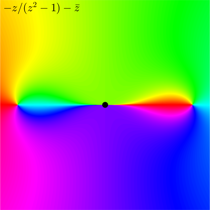
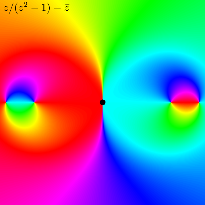
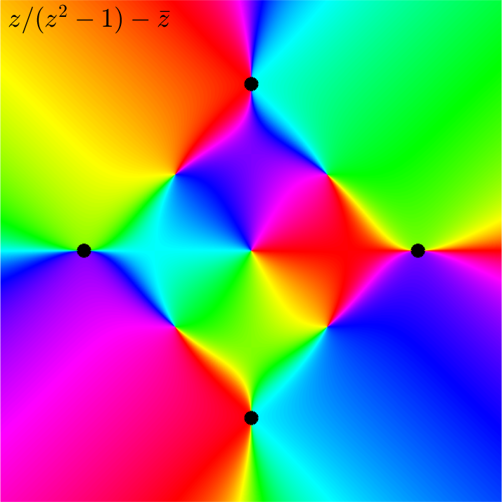
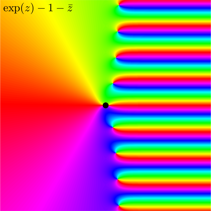
Figure 1: Phase portraits for the function in Examples 3.2–3.5. The singular zeros discussed in these examples are marked with black dots. The indices of the marked zeros are $+1$ (top left), $-1$ (top right) and $0$ (bottom row).

Example 3.2.

We show that $f(z)=h(z)-\overline{z}$ with $h(z)=-z/(z^{2}-1)$ has a singular zero with Poincaré index $+1$.

We compute the zeros of $f$. We have that $f(z)=0$ is equivalent to

$$\frac{z^{2}}{1-z^{2}}=|z^{2}|,$$ (2)

implying $z^{2}=\tfrac{|z|^{2}}{1+|z|^{2}}\geq 0$. Then (2) is equivalent to $z^{2}=z^{2}(1-z^{2})$, showing that $z_{0}=0$ is the only zero of $f$. Since

$$|h^{\prime}(z)|=\left|\frac{z^{2}+1}{(z^{2}-1)^{2}}\right|,$$ (3)

we have $|h^{\prime}(0)|=1$, so that $z_{0}$ is a singular zero of $f$.

Further, $f$ has the two simple poles $\pm 1$ with $\operatorname{ind}(f;\pm 1)=-1$; see Proposition 2.7. Combining Proposition 2.9 and Theorem 2.8, we find on a sufficiently large circle $\Gamma$

$$-1=V(f;\Gamma)=\operatorname{ind}(f;-1)+\operatorname{ind}(f;0)+\operatorname{ind}(f;1)=-2+\operatorname{ind}(f;0),$$

hence $\operatorname{ind}(f;0)=+1$. Thus $0$ is a singular zero with Poincaré index $+1$.

Example 3.3.

We show that $f(z)=h(z)-\bar{z}$ with $h(z)={z}/(z^{2}-1)$ has a singular zero with Poincaré index $-1$.

Let us compute the zeros of $f$. Clearly, $z_{0}=0$ is a zero of $f$. For $z\neq 0$, we have that $f(z)=0$ is equivalent to $(|z|^{2}-1)z^{2}=|z|^{2}$. Writing $z=\rho e^{i\varphi}$ with $\rho>0$ and $\varphi\in\mathbb{R}$, this is equivalent to $(\rho^{2}-1)e^{i2\varphi}=1$. In particular, $\rho\neq 1$ and $e^{i2\varphi}\in\mathbb{R}$, so that either $e^{i2\varphi}=-1$ or $e^{i2\varphi}=+1$. In the first case $e^{i2\varphi}=-1$ implies the contradiction $\rho=0$. In the second case $e^{i2\varphi}=1$ implies $\varphi=0,\pi$ and we find $\rho=\sqrt{2}$. Hence $f$ has the three zeros $0,\pm\sqrt{2}$. Since $|h^{\prime}(z)|$ is given by (3) we have

$$|h^{\prime}(0)|=1\quad\text{and}\quad|h^{\prime}(\pm\sqrt{2})|=3>1,$$

so that $0$ is a singular zero of $f$, and $\pm\sqrt{2}$ are sense-preserving zeros of $f$ and thus have Poincaré index $+1$ by Proposition 2.7.

Further $f$ has the two simple poles $\pm 1$ with $\operatorname{ind}(f;\pm 1)=-1$; see Proposition 2.7. Combining Proposition 2.9 and the argument principle as in Example 3.2, we find that $\operatorname{ind}(f;0)=-1$. Thus, $z_{0}=0$ is a singular zero of $f$ with Poincaré index $-1$.

Example 3.4.

We show that $f(z)=h(z)-\bar{z}$ with $h(z)=2z^{3}+\tfrac{1}{8z}$ has singular zeros with Poincaré index $0$.

We compute the zeros of $f$. Clearly, $z=0$ is a pole of $h$ and thus not a zero of $f$. Then, $f(z)=0$ is equivalent to $2z^{4}+\tfrac{1}{8}-|z|^{2}=0$. Writing $z=\rho e^{i\varphi}$, where $\rho>0$ and $\varphi\in\mathbb{R}$, we find

$$2\rho^{4}e^{i4\varphi}+\tfrac{1}{8}-\rho^{2}=0,$$ (4)

so that $e^{i4\varphi}$ is real.

Consider first the case $e^{i4\varphi}=-1$. We then have $\varphi=\tfrac{(2k+1)\pi}{4}$ with $k\in\mathbb{Z}$, and (4) becomes $2\rho^{4}+\rho^{2}-\tfrac{1}{8}=0$, implying $\rho^{2}=\tfrac{\sqrt{2}-1}{4}$. Thus, $f$ has the four zeros $z_{k}=(\tfrac{\sqrt{2}-1}{4})^{\frac{1}{2}}e^{i\frac{(2k+1)\pi}{4}}$, $k=4,5,6,7$. We determine their type. We have $h^{\prime}(z)=6z^{2}-\tfrac{1}{8z^{2}}$. A short computation yields $h^{\prime}(z_{k})=(2\sqrt{2}-1)(-1)^{k}i$. Thus $|h^{\prime}(z_{k})|>1$ and the $z_{k}$ are sense-preserving zeros of $f$. By Proposition 2.7 we have $\operatorname{ind}(f;z_{k})=+1$.

In the second case, $e^{i4\varphi}=+1$, we have $\varphi=k\tfrac{\pi}{2}$ for some $k\in\mathbb{Z}$, and equation (4) becomes $0=2\rho^{4}-\rho^{2}+\tfrac{1}{8}=2(\rho^{2}-\tfrac{1}{4})^{2}$, which yields $\rho=\tfrac{1}{2}$. Thus, $f$ has another four zeros $z_{k}=\tfrac{1}{2}e^{ik\frac{\pi}{2}}$, $k=0,1,2,3$. A short computation shows $h^{\prime}(z_{k})=(-1)^{k}$, so that these $z_{k}$ are singular zeros of $f$. We show that $z_{0},z_{1},z_{2}$, and $z_{3}$ have the same Poincaré index. Note that $f(z)=e^{i\frac{\pi}{2}}f(e^{i\frac{\pi}{2}}z)$ holds for all $z$. Denote by $\Gamma_{0}$ a small circle centered at $z_{0}$ suitable for the computation of $\operatorname{ind}(f;z_{0})$, recall Definition 2.6. Fix $k\in\{1,2,3\}$. Set $\Gamma_{k}\mathrel{\mathop{:}}=e^{ik\tfrac{\pi}{2}}\Gamma_{0}$, which then is a circle centered at $z_{k}$ with $\operatorname{ind}(f;z_{k})=V(f;\Gamma_{k})$. We find

$$\begin{split}\operatorname{ind}(f;z_{0})&=V(f;\Gamma_{0})=V(e^{ik\frac{\pi}{2}}f(e^{ik\frac{\pi}{2}}z);\Gamma_{0})=V(f(e^{ik\frac{\pi}{2}}z);\Gamma_{0})\\ &=V(f(z);\Gamma_{k})=\operatorname{ind}(f;z_{k}).\end{split}$$

Thus the singular zeros $z_{0},z_{1},z_{2}$, and $z_{3}$ of $f$ all have the same Poincaré index.

Clearly, $0$ is the only pole of $f$ and has $\operatorname{ind}(f;0)=-1$. Now, since $h(z)=(16z^{4}+1)/(8z)$ is of type $(4,1)$, we find by Proposition 2.9 and the argument principle

$$3=\operatorname{ind}(f;0)+\sum_{k=0}^{7}\operatorname{ind}(f;z_{k})=3+4\operatorname{ind}(f;z_{0}).$$

Hence $\operatorname{ind}(f;z_{k})=0$ for $k=0,1,2,3$, and we have shown that $f$ has singular zeros with Poincaré index $0$.

Example 3.5.

Let $f(z)=h(z)-\overline{z}=e^{z}-1-\overline{z}$, which has an isolated zero at the origin. Since $|h^{\prime}(0)|=e^{0}=1$, it is a singular zero. The phase portrait (Figure 1) indicates that $f$ has index $0$, but determining the index as in the previous examples is not possible.

All these computations were quite laborious. With our main results Theorems 4.2 and 4.6 below, we will be able to compute these indices very easily by looking at the power series of the analytic part; see Section 4.3.

4 Determining the index from the power series

Let $f(z)=h(z)-\overline{z}$ be a complex-valued harmonic function, where $h$ is an analytic function. We aim to characterize the index of $f$ at an isolated zero $z_{0}$ by the coefficients of the Taylor series of $h$ at $z_{0}$. For regular zeros $z_{0}$, the index can be easily inferred from the series, which is a direct consequence of Definition 2.1, and Theorem 3.1.

Proposition 4.1.

Let $f(z)=h(z)-\overline{z}$, with $h$ analytic, have a zero at $z_{0}\in\mathbb{C}$, so that

$$f(z)=h(z)-\overline{z}=\sum_{k=1}^{\infty}a_{k}(z-z_{0})^{k}-\overline{z-z_{0}}$$

near $z_{0}$.

1. If $|a_{1}|>1$ the function $f$ is sense-preserving at $z_{0}$ and $\operatorname{ind}(f;z_{0})=+1$.

2. If $|a_{1}|<1$ the function $f$ is sense-reversing at $z_{0}$ and $\operatorname{ind}(f;z_{0})=-1$.

4.1 Determining the index of singular zeros

The preceding proposition shows that the index of a regular zero is determined by the first term of the Taylor series of $h$. The case of a singular zero is more subtle than that of a regular zero, and the occurrence of a singular zero is typically excluded in the published literature on harmonic mappings. However, as we will see in the following theorem, the index of a singular zero is determined from the leading terms in the Taylor series of $h$ as well.

Theorem 4.2.

Let the complex-valued harmonic function

$$f(z)=h(z)-\overline{z}=z+\sum_{k=2}^{\infty}a_{k}z^{k}-\overline{z}$$

have an isolated singular zero at the origin. Let $n\geq 2$ be the smallest index with $a_{n}\neq 0$, then

$$\operatorname{ind}(f;0)=\begin{cases}\phantom{+}0&\operatorname{Re}(a_{n})\neq 0,\;n\,\text{even}\\ +1&\operatorname{Re}(a_{n})>0,\;n\,\text{odd}\\ -1&\operatorname{Re}(a_{n})<0,\;n\,\text{odd}\end{cases}.$$

Remark 4.3.

Recall from Proposition 4.1 that the index of a regular zero $z_{0}$ of $h(z)-\overline{z}$ is completely determined by the first derivative of $h$ at $z_{0}$. If $z_{0}$ is singular, the index is, except for the case $\operatorname{Re}(a_{n})=0$, completely determined by the first two non-vanishing derivatives of $h$ at $z_{0}$.

Remark 4.4.

The only case not covered by Theorem 4.2 is that of a purely imaginary coefficient $a_{n}$. No characterization of the index is given in this case (of course it still is in $\{0,\pm 1\}$). We have constructed examples showing that in this particular case the first two non-vanishing derivatives are not sufficient to characterize the index at $0$. This behaviour is illustrated in Section 5. Hence a complete characterization requires local or global information about $h$ beyond of what is used in Theorem 4.2.

Remark 4.5.

For harmonic polynomials of the special form

$$f(z)=z+a_{n}z^{n}-\overline{z},\quad a_{n}\neq 0,$$

we give a complete characterization of the index of $f$ at $0$ in Lemma 4.12, that is, including the aforementioned case $\operatorname{Re}(a_{n})=0$. As it turns out, the index in $0$ is always $+1$ for these functions if $a_{n}$ is purely imaginary.

Theorem 4.2 makes two normalization assumptions, neither of which is restrictive. The first one asserts that the singular zero of interest is in the origin. If $z_{0}$ is any zero of $f$, then $0=h(z_{0})-\overline{z_{0}}$, and expanding $h$ in a power series yields

$$f(z)=\sum_{k=1}^{\infty}a_{k}(z-z_{0})^{k}-\overline{z-z_{0}}.$$

After the change of variables $w=z-z_{0}$, the zero is at the origin, and the index does not change.

The second normalization is $a_{1}=1$. To see that this is not a restriction, consider for an arbitrary $a_{1}\neq 0$ the function

$$f(z)=h(z)-\overline{z}=a_{1}z+\sum_{k=2}^{\infty}a_{k}z^{k}-\overline{z},$$

and suppose that it has an isolated singular zero at $z_{0}=0$. This implies $|a_{1}|=|h^{\prime}(0)|=1$, so that $a_{1}=e^{i\theta}$ for some $\theta\in\mathbb{R}$. From

$$e^{-i\theta/2}f(z)=e^{i\theta/2}z+\sum_{k=2}^{\infty}a_{k}e^{-i(k+1)\theta/2}(e^{i\theta/2}z)^{k}-\overline{e^{i\theta/2}z}$$

we find

$$V(f;\Gamma)=V(e^{-i\theta/2}f(z);\Gamma)=V(e^{-i\theta/2}f(e^{-i\theta/2}z);\Gamma)$$

for all sufficiently small circles $\Gamma$. Therefore $f$ and $z+\sum_{k=2}^{\infty}a_{k}e^{-i(k+1)\theta/2}z^{k}-\overline{z}$ have the same index at the origin, and we can assume $a_{1}=1$. Substituting back, we can reformulate Theorem 4.2 without the discussed normalizations.

Theorem 4.6.

Let the complex-valued harmonic function

$$f(z)=h(z)-\overline{z}$$

with analytic $h$ have an isolated singular zero at $z_{0}\in\mathbb{C}$, and $h^{\prime}(z_{0})=e^{i\theta}$. Let $n\geq 2$ be the smallest index with $h^{(n)}(z_{0})=ce^{i\varphi}\neq 0$, where $c>0$, and set

$$\eta\mathrel{\mathop{:}}=\cos(\varphi-\tfrac{n+1}{2}\theta),$$ (5)

then

$$\operatorname{ind}(f;z_{0})=\begin{cases}\phantom{+}0&\eta\neq 0,\;n\text{ even}\\ +1&\eta>0,\;n\text{ odd}\\ -1&\eta<0,\;n\text{ odd}\end{cases}.$$

4.2 Proof of Theorem 4.2

Throughout we consider the complex-valued harmonic function

$$f(z)=h(z)-\overline{z}=z+\sum_{k=2}^{\infty}a_{k}z^{k}-\overline{z},$$

which has a singular zero at the origin, and we assume that the zero is isolated. Then not all coefficients $a_{k}$ with $k\geq 2$ can vanish: If $a_{k}=0$ for all $k\geq 2$, then $f(z)=z-\overline{z}$, which vanishes on the whole real line, so that $0$ is not an isolated zero. Further we denote by $n\geq 2$ the smallest integer satisfying $a_{n}\neq 0$. We thus have

$$f(z)=z+a_{n}z^{n}+\sum_{k=n+1}^{\infty}a_{k}z^{k}-\overline{z},\quad a_{n}\neq 0.$$ (6)

The proof of Theorem 4.2 is divided in several steps, and an outline is as follows.

1. We show that $f$ and $z+a_{n}z^{n}-\overline{z}$ have the same index at $0$ (Lemma 4.8).

2. We show that $a_{n}$ can be reduced to one of $\pm 1,\pm i$ (Lemmas 4.9 and 4.10).

3. We show that then $n$ can be replaced by $2$ when $n$ is even and by $3$ when $n$ is odd (Lemma 4.11).

4. We explicitly compute the index in each of these cases (Lemma 4.12).

We begin by showing that the series (6) can be truncated after the first non-vanishing coefficient without changing the index (Lemma 4.8 below). For this we need the following technical, preparatory lemma.

Lemma 4.7.

Let

$$g(z)=az^{n}+z-\overline{z}$$

where $n\geq 2$ and $a\neq 0$, and let $0<c<1$. If $\operatorname{Re}(a)\neq 0$, then

$$|g(z)|>c|\operatorname{Re}(a)|\rho^{n}\quad\text{on}\quad|z|=\rho$$ (7)

and if $\operatorname{Re}(a)=0$

$$|g(z)|>c\frac{n}{2}|a|^{2}\rho^{2n-1}\quad\text{on}\quad|z|=\rho$$ (8)

for all sufficiently small $\rho$.

Proof.

Fix $0<c<1$, and write $z=\rho e^{it}$ with $\rho>0$ and $t\in[0,2\pi]$. Then

$$|g(z)|=|a\rho^{n}e^{int}+2i\rho\sin(t)|=\rho^{n}|ae^{int}+\frac{2i}{\rho^{n-1}}\sin(t)|.$$

The absolute value on the right hand side is the distance between the curve $\sigma(t)=\frac{2i}{\rho^{n-1}}\sin(t)$ and the circle $\gamma(t)=-ae^{int}$. We show that these curves have always the required distance. Define $\delta>0$ by $\delta=c|\operatorname{Re}(a)|$ for $\operatorname{Re}(a)\neq 0$ and $\delta=c\frac{n}{2}|a|^{2}\rho^{n-1}$ if $\operatorname{Re}(a)=0$. Then $\delta<|a|$ for sufficiently small $\rho$.

Figure 2: Illustration for the proof of Lemma 4.7. The thick line is the location of the sine term for $t$ satisfying (9).

Let first $t\in[0,\pi/2]$. Then $\sigma(t)$ moves from $0$ to $2i/\rho^{n-1}$ and thus crosses the circle with center $0$ and radius $|a|$; see Figure 2. We determine at which time $t\in[0,\pi/2]$ we have

$$\frac{2}{\rho^{n-1}}\sin(t)=|a|+\tau,\quad-\delta\leq\tau\leq\delta.$$ (9)

For $t\in[0,\pi/2]$ not satisfying (9) we have $|\sigma(t)-\gamma(t)|>\delta$, so that (7) or (8) is satisfied. Equation (9) is equivalent to

$$\sin(t)=\frac{|a|+\tau}{2}\rho^{n-1},\quad-\delta\leq\tau\leq\delta.$$

For sufficiently small $\rho$ the values are close to zero so that

$$t=\frac{|a|+\tau}{2}\rho^{n-1}+\mathcal{O}(\rho^{3n-3}),\quad-\delta\leq\tau\leq\delta.$$ (10)

Since $|g(z)|\geq|\operatorname{Re}(g(z))|$, we bound the real part of $g$:

$$\operatorname{Re}(g(z))=\operatorname{Re}(a\rho^{n}e^{int})=\operatorname{Re}(a)\rho^{n}\cos(nt)-\operatorname{Im}(a)\rho^{n}\sin(nt).$$

Note that $t$ in (10) is of order $\mathcal{O}(\rho^{n-1})$, so that

$$\operatorname{Re}(g(z))=\operatorname{Re}(a)\rho^{n}-\operatorname{Im}(a)n\rho^{n}t+\mathcal{O}(\rho^{2n}).$$ (11)

Let $\operatorname{Re}(a)\neq 0$. Inserting $t$ from (10) in (11) gives

$$\operatorname{Re}(g(z))=\operatorname{Re}(a)\rho^{n}+\mathcal{O}(\rho^{2n-1}),$$

so that

$$|g(z)|=|\operatorname{Re}(a)|\rho^{n}+\mathcal{O}(\rho^{2n-1})>c|\operatorname{Re}(a)|\rho^{n}$$

for all sufficiently small $\rho$. Inserting $t$ from (10) in (11) when $\operatorname{Re}(a)=0$ gives

$$\operatorname{Re}(g(z))=-\operatorname{Im}(a)\frac{n}{2}(|a|+\tau)\rho^{2n-1}+\mathcal{O}(\rho^{2n}),$$

and

$$\begin{split}|g(z)|&\geq|\operatorname{Im}(a)|\frac{n}{2}(|a|+\tau)\rho^{2n-1}+\mathcal{O}(\rho^{2n})\\ &\geq|\operatorname{Im}(a)|\frac{n}{2}(|a|-\delta)\rho^{2n-1}+\mathcal{O}(\rho^{2n})>c\frac{n}{2}|a|^{2}\rho^{2n-1}\end{split}$$

for all sufficiently small $\rho$. (Recall that $\delta$ is of order $\rho^{n-1}$ in this case.)

As a next step, let $t\in[\pi/2,\pi]$. We apply the same reasoning and determine all $t$ with (9). Let $s=\pi-t\in[0,\pi/2]$. Then $\sin(s)=\sin(t)$, and $s$ satisfies (10). Further, $|\operatorname{Re}(a\rho^{n}e^{int})|=|\operatorname{Re}(a\rho^{n}e^{-isn})|$. Note that switching the sign of $t$ in the previous case does not alter the proof, so we obtain again (7) and (8).

For $t\in[\pi,2\pi]$ the sine is negative, so (9) has to be replaced by

$$\frac{2}{\rho^{n-1}}\sin(t)=-|a|-\tau,\quad-\delta\leq\tau\leq\delta,$$

with $\delta$ as before. For $t\in[\pi,3\pi/2]$ the substitution $s=t-\pi\in[0,\pi/2]$ brings us back to the first case $t\in[0,\pi/2]$, so that we obtain (7) and (8). For $t$ in $[3\pi/2,2\pi]$ we substitute $s=2\pi-t\in[0,\pi/2]$ so that $\sin(t)=-\sin(s)$ and $s$ satisfies (9). As in the second case $\operatorname{Re}(a\rho^{n}e^{int})=\operatorname{Re}(a\rho^{n}e^{-isn})$, and we obtain (7) and (8). ∎

The following lemma shows that the index of $f$ at the origin depends on the first two nonvanishing coefficients in the Taylor series of $h$.

Lemma 4.8.

Let

$$f(z)=h(z)-\overline{z}=z+a_{n}z^{n}+\sum_{k=n+1}^{\infty}a_{k}z^{k}-\overline{z}$$

with $\operatorname{Re}(a_{n})\neq 0$. Then $f$ and

$$g(z)=z+a_{n}z^{n}-\overline{z}$$

have the same index at the origin: $\operatorname{ind}(f;0)=\operatorname{ind}(g;0)$.

Proof.

We aim to apply Rouché’s theorem on a sufficiently small circle around the origin. Let $R>0$ be smaller than the radius of convergence of the power series of $h$ at $0$, and so that no further zeros of $f$ and $g$ are contained in the closed $R$-disk. In particular $M=\sum_{k=n+1}^{\infty}a_{k}R^{k-(n+1)}<\infty$. Let $0<\rho<R$. We then have for $|z|=\rho$

$$|f(z)-g(z)|=|\sum_{k=n+1}^{\infty}a_{k}z^{k}|\leq\rho^{n+1}\sum_{k=n+1}^{\infty}|a_{k}|\rho^{k-(n+1)}=\rho^{n+1}M.$$

Together with the bound from Lemma 4.7 we obtain the strict inequality

$$|f(z)-g(z)|\leq\rho^{n+1}M<c|\operatorname{Re}(a_{n})|\rho^{n}<|g(z)|\leq|g(z)|+|f(z)|$$

for all sufficiently small $\rho$, so that $f$ and $g$ have the same winding along $|z|=\rho$ by Rouché’s theorem, showing the assertion. ∎

The next lemma shows that scaling the coefficient $a_{n}$ does not change the index.

Lemma 4.9.

Let $n\geq 2$ and let $a,b\in\mathbb{C}$ be nonzero with same argument. Then $g(z)=az^{n}+z-\overline{z}$ and $\widetilde{g}(z)=bz^{n}+z-\overline{z}$ have the same index at the origin: $\operatorname{ind}(g;0)=\operatorname{ind}(\widetilde{g};0)$.

Proof.

Let $\gamma(t)=\rho e^{it}$ with $t\in[0,2\pi]$. We show that the curves $g\circ\gamma$ and $\widetilde{g}\circ\gamma$ are homotopic in $\mathbb{C}\backslash\{0\}$ for all sufficiently small $\rho$. Define

$$H(t,s)=sg(\gamma(t))+(1-s)\widetilde{g}(\gamma(t)),\quad(t,s)\in[0,2\pi]\times[0,1].$$

Note that $H(0,s)=H(2\pi,s)$ for all $s$, i.e., $H(\cdot,s)$ is a closed curve for each $s$. Writing $a=|a|e^{i\varphi}$ and $b=|b|e^{i\varphi}$ (they have the same argument by assumption) gives

$$H(t,s)=(s|a|+(1-s)|b|)\rho^{n}e^{i(nt+\varphi)}+2i\rho\sin(t),$$

and we have to show that $H(t,s)$ is nonzero for all $(t,s)$ and for all sufficiently small $\rho$. If $t$ is a multiple of $\pi$, we have

$$|H(k\pi,s)|=(s|a|+(1-s)|b|)\rho^{n}>0,\quad k=0,1,2.$$

For $t\neq 0,\pi,2\pi$ the term $2i\rho\sin(t)$ is nonzero and purely imaginary. For $H(t,s)$ to become zero, the first term $(s|a|+(1-s)|b|)\rho^{n}e^{i(nt+\varphi)}$ must thus also be imaginary, which can happen at at most finitely many values of $t$ (independent of $s$). At each such point, making $\rho$ sufficiently small guarantees that $H(t,s)\neq 0$. Thus $H(t,s)\neq 0$ for all $(t,s)$ and all sufficiently small $\rho$, which shows that the curves $g\circ\gamma$ and $\widetilde{g}\circ\gamma$ are homotopic in $\mathbb{C}\backslash\{0\}$ and thus have the same winding. Since this holds for all sufficiently small $\rho$, we obtain $\operatorname{ind}(g;0)=\operatorname{ind}(\widetilde{g};0)$. ∎

The previous lemma shows that the index of $g(z)=az^{n}+z-\overline{z}$ at the origin is the same for all $a$ on a ray starting in the origin. Next we show that the index is also the same if we displace $a$ in its (open) half-plane.

Lemma 4.10.

Let $n\geq 2$ and $\operatorname{Re}(a)\neq 0$. Then the functions $g(z)=az^{n}+z-\overline{z}$ and $\widetilde{g}(z)=\operatorname{sign}(\operatorname{Re}(a))z^{n}+z-\overline{z}$ have the same index at the origin: $\operatorname{ind}(g;0)=\operatorname{ind}(\widetilde{g};0)$.

Proof.

Let $a\in\mathbb{C}$ with $\operatorname{Re}(a)>0$ and write $g_{a}(z)=az^{n}+z-\overline{z}$ and $g_{1}(z)=z^{n}+z-\overline{z}$. Let $\gamma(t)=\rho e^{it}$ with $\rho>0$. We show that the closed curves $g_{a}\circ\gamma$ and $g_{1}\circ\gamma$ are homotopic in $\mathbb{C}\backslash\{0\}$, provided that $\rho$ is sufficiently small. Define

$$H(t,s)=sg_{a}(\gamma(t))+(1-s)g_{1}(\gamma(t)),\quad(t,s)\in[0,2\pi]\times[0,1],$$

which satisfies $H(0,s)=H(2\pi,s)$ for all $s$, i.e., each $H(\cdot,s)$ is a closed curve. Since

$$H(t,s)=(1+s(a-1))(\gamma(t))^{n}+\gamma(t)-\overline{\gamma(t)},$$

Lemma 4.7 shows that for all $t$ and all sufficiently small $\rho$

$$|H(t,s)|\geq c|\operatorname{Re}(1+s(a-1))|\rho^{n}\geq c\min\{1,\operatorname{Re}(a)\}\rho^{n}>0,$$

so that $|H(t,s)|>0$ for all $(t,s)$ and sufficiently small $\rho$. This shows that $g_{a}\circ\gamma$ and $g_{1}\circ\gamma$ are homotopic in $\mathbb{C}\backslash\{0\}$, so that $g_{a}$ and $g_{1}$ have the same winding along $|z|=\rho$. Since this holds for all sufficiently small $\rho$, their indices are the same. Note that we needed that $a$ and $1$ are on the same side of the imaginary axis, so that $H(t,s)$ is guaranteed to be nonzero. Similarly $g_{a}$ with $\operatorname{Re}(a)<0$ and $g_{-1}$ are homotopic in $\mathbb{C}\backslash\{0\}$. ∎

The next lemma shows that to compute the index of $az^{n}+z-\overline{z}$ at the origin, we can reduce the power $n$ in steps of $2$, provided that $\operatorname{Re}(a)\neq 0$.

Lemma 4.11.

Let $n\geq 2$ and $\operatorname{Re}(a)\neq 0$. Then $g(z)=az^{n+2}+z-\overline{z}$ and $\widetilde{g}(z)=az^{n}+z-\overline{z}$ have the same index at the origin.

Proof.

We show that $g(z)=az^{n+2}+z-\overline{z}$ and $\widetilde{g}(z)=az^{n}+z-\overline{z}$ have the same winding on all sufficiently small circles around the origin using Rouché’s Theorem 2.5.

We can assume that $a=\pm 1$ by Lemma 4.10. Write $z=\rho e^{it}$ with $\rho>0$ and $t\in[0,2\pi]$. To apply Rouché’s theorem, we wish to show the inequality

$$|\widetilde{g}(z)-g(z)|=|a\rho^{n}e^{int}-a\rho^{n+2}e^{i(n+2)t}|<|\widetilde{g}(z)|=|a\rho^{n}e^{int}+2i\rho\sin(t)|$$

for all $0\leq t\leq 2\pi$, or equivalently

$$|\rho^{n-1}-\rho^{n+1}e^{i2t}|^{2}<|a\rho^{n-1}e^{int}+2i\sin(t)|^{2},\quad 0\leq t\leq 2\pi,$$ (12)

for all sufficiently small $\rho>0$. The left and right hand sides in (12) are

$$\begin{split}|\rho^{n-1}-\rho^{n+1}e^{i2t}|^{2}&=\rho^{2n-2}-2\rho^{2n}\cos(2t)+\rho^{2n+2},\\ |a\rho^{n-1}e^{int}+2i\sin(t)|^{2}&=\rho^{2n-2}+4a\rho^{n-1}\sin(t)\sin(nt)+4\sin(t)^{2},\end{split}$$

respectively. Thus (12) is equivalent to

$$F(t)\mathrel{\mathop{:}}=4\sin(t)^{2}+4a\rho^{n-1}\sin(t)\sin(nt)+2\rho^{2n}\cos(2t)-\rho^{2n+2}>0$$ (13)

for all $t\in[0,2\pi]$ and all sufficiently small $\rho>0$.

Fix $0<\delta<\frac{\pi}{4}$, so that $\cos(2\delta)>0$ and $\sin(\delta)>0$. For $|t|\leq\delta$ and $|t-\pi|\leq\delta$ we compute

$$F(t)=4\sin(t)^{2}\left(1+a\rho^{n-1}\frac{\sin(nt)}{\sin(t)}\right)+\rho^{2n}(2\cos(2t)-\rho^{2}).$$

Note that $|a\sin(nt)/\sin(t)|\leq M<\infty$ on $[-\delta,\delta]$ and $[\pi-\delta,\pi+\delta]$, since $t=0$ and $t=\pi$ are removable singularities. Therefore,

$$F(t)\geq 4\sin(t)^{2}(1-M\rho^{n-1})+\rho^{2n}(2\cos(2\delta)-\rho^{2}),$$

which is positive for all sufficiently small $\rho>0$. For $\delta\leq t\leq\pi-\delta$ and $\pi+\delta\leq t\leq 2\pi-\delta$ we have $\sin(t)^{2}\geq\sin(\delta)^{2}>0$, so that $F(t)\geq 4\sin(\delta)^{2}+\mathcal{O}(\rho)$, which is positive for all sufficiently small $\rho>0$.

This establishes (13) for all $t\in[0,2\pi]$ and all sufficiently small $\rho>0$, so that $\operatorname{ind}(g;0)=\operatorname{ind}(\widetilde{g};0)$ by Rouché’s theorem. ∎

The next lemma completely characterizes the index of the harmonic polynomials $az^{n}+z-\overline{z}$ at the origin, for all $n\geq 2$ and all nonzero $a$.

Lemma 4.12.

Let $g(z)=az^{n}+z-\overline{z}$ with nonzero $a\in\mathbb{C}$ and $n\geq 2$. We then have for even $n$

$$\operatorname{ind}(g;0)=\begin{cases}0&\operatorname{Re}(a)\neq 0\\ 1&\operatorname{Re}(a)=0\end{cases},$$

and for odd $n$

$$\operatorname{ind}(g;0)=\begin{cases}+1&\operatorname{Re}(a)\geq 0\\ -1&\operatorname{Re}(a)<0\end{cases}.$$

Proof.

We treat the cases $\operatorname{Re}(a)\neq 0$ and $\operatorname{Re}(a)=0$ separately.

Case $\bm{\operatorname{Re}(a)\neq 0$}.$

We distinguish the cases of even and odd $n$. First, let $n$ be even, so that we can assume $n=2$ by Lemma 4.11. By Lemma 4.10 we can even assume that $a\neq 0$ is real (and even $\pm 1$).

We compute the zeros of $g(z)=az^{2}+z-\overline{z}$. Writing $z=x+iy$ with $x,y\in\mathbb{R}$ we find

$$g(z)=a(x+iy)^{2}+2iy=a(x^{2}-y^{2})+2i(axy+y).$$

Thus $g(z)=0$ if and only if

$$x^{2}-y^{2}=0\quad\text{and}\quad y(ax+1)=0.$$

The second equation is zero if $y=0$ (thus $x=0$) or $ax+1=0$, i.e., $x=-1/a$ and thus $y=\pm 1/a$. This gives the three solutions $z_{0}=0$, $z_{+}=(-1+i)/a$ and $z_{-}=(-1-i)/a$, and we compute their indices. Let $h(z)=az^{2}+z$. Then $|h^{\prime}(z_{\pm})|=|-1\pm 2i|>1$ shows that $z_{\pm}$ are sense-preserving zeros, so that $\operatorname{ind}(g;z_{\pm})=1$ by Proposition 4.1.

On a sufficiently large circle $\Gamma$, the winding of $g$ is $2$ by Proposition 2.9. Applying the argument principle 2.8 on $\Gamma$ shows

$$2=V(g;\Gamma)=\operatorname{ind}(g;z_{+})+\operatorname{ind}(g;z_{-})+\operatorname{ind}(g;0)=2+\operatorname{ind}(g;0),$$

i.e., $\operatorname{ind}(g;0)=0$. This concludes the case of $\operatorname{Re}(a)\neq 0$ and even $n$.

Next we consider the case $\operatorname{Re}(a)\neq 0$ and $n$ odd. By Lemma 4.11 we can assume that $n=3$. Note that the winding of $g(z)=az^{3}+z-\overline{z}$ around a sufficiently large circle is $3$. Let $h(z)=az^{3}+z$. As before, let $z=x+iy$ with real $x$ and $y$, and compute the zeros of $g$ explicitly.

For real $a>0$ we find the three zeros

$$z_{0}=0,\quad z_{\pm}=\pm i\sqrt{2/a}.$$

Since $|h^{\prime}(z_{\pm})|=5>1$, the zeros $z_{+}$ and $z_{-}$ are sense-preserving and have index $+1$. The argument principle applied on a sufficiently large circle now shows that $\operatorname{ind}(g;0)=+1$. Lemma 4.10 shows that $\operatorname{ind}(g;0)=+1$ for all $a$ with $\operatorname{Re}(a)>0$.

For real $a<0$ we find the five zeros

$$z_{0}=0,\quad z_{\pm}=\pm\sqrt{\sqrt{3}/(4|a|)}+i\sqrt{1/(4|a|)},\quad\overline{z_{\pm}}.$$

A short computation gives $|h^{\prime}(z_{\pm})|=|h^{\prime}(\overline{z_{\pm}})|>1$, so that these zeros have index $+1$ by Proposition 4.1. Finally, the argument principle applied to a sufficiently large circle implies $\operatorname{ind}(g;0)=-1$. Lemma 4.10 shows that $\operatorname{ind}(g;0)=-1$ for all $a$ with $\operatorname{Re}(a)<0$. This concludes the case $\operatorname{Re}(a)\neq 0$ and odd $n$.

Case $\bm{\operatorname{Re}(a)=0}$.

By Lemma 4.9 we can assume that $a=\pm i$ and we treat the case $a=i$ first. We explicitly compute the zeros of $g(z)=iz^{n}+z-\overline{z}$. Let $z=\rho e^{i\varphi}$ with $\rho>0$ and $\varphi\in[0,2\pi[$. Then $g(z)=0$ is equivalent to

$$\rho^{n-1}e^{in\varphi}+2\sin(\varphi)=0,$$

and considering the real and imaginary parts separately we obtain the pair of equations

$$\rho^{n-1}\cos(n\varphi)+2\sin(\varphi)=0,$$ (14)

$$\rho^{n-1}\sin(n\varphi)=0.$$ (15)

Equation (15) is equivalent to $n\varphi=k\pi$ with $k\in\mathbb{Z}$, giving the angles

$$\varphi_{k}=k\frac{\pi}{n},\quad k=0,1,2,\ldots,2n-1.$$

Inserting these in (14) gives

$$\rho^{n-1}=(-1)^{k+1}2\sin\left(k\frac{\pi}{n}\right)$$ (16)

which must be positive. In particular, $k=0,n,2n$ are not admissible. For $k=1,2,\ldots,n-1$ the sine is positive, and thus $k$ must be odd, and for $k=n+1,n+2,\ldots,2n-1$, the sine is negative and thus $k$ must be even. Let us count precisely the number of admissible angles. First, let $n$ be even. Then $k=1,3,\ldots,n-1$, give $n/2$ solutions, and $k=n+2,n+4,\ldots,2n-2$ give another $n/2-1$ solutions. Second, let $n$ be odd. Then $k=1,3,\ldots,n-2$ give $(n-1)/2$ solutions, and $k=n+1,n+3,\ldots,2n-2$ are $(n-1)/2$ solutions.

In either case we thus have $n-1$ zeros $z_{k}=\rho_{k}e^{i\varphi_{k}}$, where $\rho_{k}$ is given by (16), and we show that these are sense-preserving. Let $h(z)=iz^{n}+z$. We then have

$$\begin{split}|h^{\prime}(z_{k})|&\geq|inz_{k}^{n-1}|-1=\left|in(-1)^{k+1}2\sin\left(k\frac{\pi}{n}\right)e^{i(n-1)\varphi_{k}}\right|-1\\ &=2n\left|\sin\left(k\frac{\pi}{n}\right)\right|-1\geq 2n\sin(\pi/n)-1\geq 4-1>1.\end{split}$$

In the last estimate we used that $\pi\geq\sin(\pi x)/x\geq 2$ for $x\in[0,1/2]$, readily established by basic calculus. Therefore these $n-1$ zeros are sense-preserving and have index $+1$. Since the winding of $g$ on a sufficiently large circle is $n$, this implies $\operatorname{ind}(g;0)=+1$.

It remains to consider the case $a=-i$. The function $g(z)=-iz^{n}+z-\overline{z}$ has a zero at the origin. As in the case $a=i$ we explicitly compute all other zeros and show that they are regular. Writing $z=\rho e^{i\varphi}$, we find that $g(z)=0$ is equivalent to

$$\rho^{n-1}e^{in\varphi}-2\sin(\varphi)=0,$$

which gives again the angles $\varphi_{k}=k\pi/n$, $k=0,1,\ldots,2n-1$, and the corresponding radii

$$\rho_{k}^{n-1}=(-1)^{k}2\sin\left(k\frac{\pi}{n}\right).$$

(Note the flipped sign compared to the case $a=i$.) Now, for $k=1,2,\ldots,n-1$ we must have $k$ even, and for $k=n+1,\ldots,2n-1$ we must have $k$ odd. In each case we find again $n-1$ solutions. The same computation as before shows $|h^{\prime}(z_{k})|>3$, so that the $n-1$ zeros are sense-preserving with index $+1$, implying $\operatorname{ind}(g;0)=1$ as before. ∎

With Lemma 4.12 we have completed the proof of Theorem 4.2.

4.3 The examples revisited

In the previous Section 3.1 we had shown various examples of functions $f$ having a singular zero $z_{0}$, and we computed their indices. The cumbersome computation entailed the determination of the winding on a sufficiently large circle that encloses all exceptional points of $f$, and determining the index of all such points except for $z_{0}$. We then used the argument principle to finally determine the index of $z_{0}$.

Using Theorem 4.2 we are now able to compute these indices directly. For Example 3.2, where $f(z)=z/(1-z^{2})-\overline{z}$ has a singular zero in $0$, we find

$$\frac{z}{1-z^{2}}=z+z^{3}+\mathcal{O}(z^{5}),$$ (17)

so that the first non-vanishing power after $z$ in the series expansion is $n=3$, with corresponding coefficient $a_{3}=1$. Hence, by our classification, the index is $+1$. From the series expansion (17) one also finds that the index of the isolated singular zero $0$ of $f(z)=-z/(1-z^{2})$ is $-1$ (cf. Example 3.3).

In Example 3.4 we considered the function $f(z)=2z^{3}+1/(8z)-\overline{z}$, and we found that $z_{0}=i/2$ is one out of four singular zeros having index $0$. We develop the analytic part of $f$ in a power series around $z_{0}$, i.e.,

$$2z^{3}+\frac{1}{8z}=\frac{i}{2}-\left(z-\frac{i}{2}\right)+4i\left(z-\frac{i}{2}\right)^{2}+\mathcal{O}\left(\left(z-\frac{i}{2}\right)^{4}\right).$$

In contrast to the previous example, the coefficients in this expansion are not normalized as in Theorem 4.2, so we resort to the general form of our characterization, given in Theorem 4.6. We have $a_{1}=-1=e^{i\theta}$ with $\theta=\pi$, and $0\neq a_{2}=4i=4e^{i\varphi}$, with $\varphi=\pi/2$, so that $\eta=\cos(\pi/2-3/2\pi)=-1$ (see definition (5)). Since $n=2$ is even and $\eta\neq 0$ we obtain $\operatorname{ind}(f;i/2)=0$.

In the final Example 3.5 we considered the function $f(z)=\exp(z)-1-\overline{z}$. Lacking of tools to compute the index of the singular zero $z_{0}=0$, we resorted to the phase portrait of $f$ (see Figure 1), from which we read that the index should be zero. Developing $\exp(z)-1$ in a series around the origin, i.e.,

$$\exp(z)-1=z+\frac{z^{2}}{2}+\mathcal{O}(z^{3}),$$

we see that $n=2$ is the first non-vanishing power, and that the corresponding coefficient is $a_{2}=1/2$. From the classification in Theorem 4.2 it follows that $\operatorname{ind}(f;0)=0$.

5 Conclusions and future work

In this work we developed a technique to determine the index of singular zeros of $f(z)=h(z)-\overline{z}$. In summary, this index depends only on the first two non-vanishing coefficents of the power series of $h$ at the zero. Our classification is almost always applicable. As discussed in the Remarks 4.3–4.5, we had to exclude one particular coefficient configuration from our classification. The reason is that in this case the index $\operatorname{ind}(f;z_{0})$ is not entirely defined by these first two coefficients.

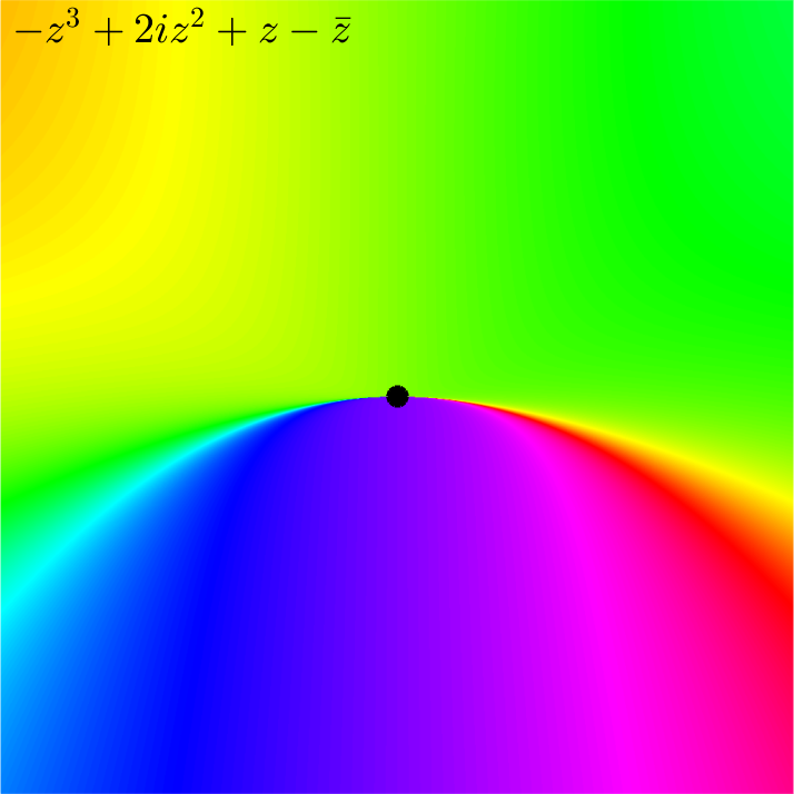
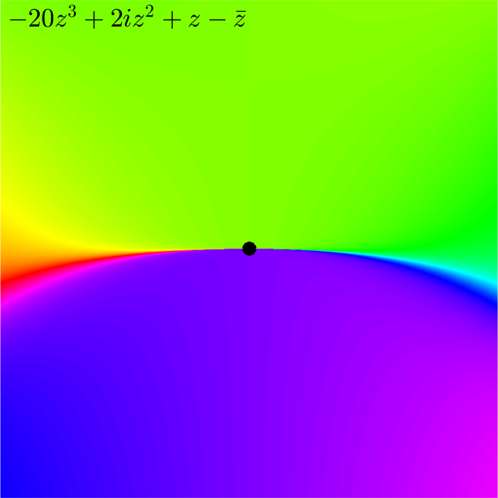
Figure 3: An example for the excluded case in Theorem 4.2; see Section 5.

In order to illustrate this behaviour, consider the functions

$$f_{1}(z)=-z^{3}+iz^{2}+z-\overline{z}\quad\text{and}\quad f_{2}(z)=-20z^{3}+iz^{2}+z-\overline{z},$$

which are shown in Figure 3. Both functions have a singular zero at the origin, and their Taylor series up to order two is identical. Since the coefficient $a_{2}=2i$ is purely imaginary, our classification in Theorem 4.2 does not apply. Indeed their indices at $0$ are $+1$ and $-1$, implying that the first two coefficients are not sufficient to determine the index. Our preliminary investigation of this case, i.e., where the second non-vanishing coefficient is purely imaginary, has led us to the belief that this situation is much more irregular, and that a thorough investigation is to be carried out in future work.

Another interesting extension of our results would be the consideration of a general anti-analytic part, i.e., general harmonic mappings $f=h+\overline{g}$. Since the index is a local property in this case as well, one could hope that a similarly flavoured characterization can be obtained in this general setting.

preprint tandf

References

- [1] M. B. Balk, Polyanalytic functions, vol. 63 of Mathematical Research, Akademie-Verlag, Berlin, 1991.
- [2] J. B. Conway, Functions of one complex variable, vol. 11 of Graduate Texts in Mathematics, Springer-Verlag, New York-Berlin, second ed., 1978.
- [3] P. Duren, Harmonic mappings in the plane, vol. 156 of Cambridge Tracts in Mathematics, Cambridge University Press, Cambridge, 2004, http://dx.doi.org/10.1017/CBO9780511546600.
- [4] P. Duren, W. Hengartner, and R. S. Laugesen, The argument principle for harmonic functions, Amer. Math. Monthly, 103 (1996), pp. 411–415, http://dx.doi.org/10.2307/2974933.
- [5] L. Geyer, Sharp bounds for the valence of certain harmonic polynomials, Proc. Amer. Math. Soc., 136 (2008), pp. 549–555, http://dx.doi.org/10.1090/S0002-9939-07-08946-0.
- [6] D. Khavinson and G. Neumann, On the number of zeros of certain rational harmonic functions, Proc. Amer. Math. Soc., 134 (2006), pp. 1077–1085, http://dx.doi.org/10.1090/S0002-9939-05-08058-5.
- [7] D. Khavinson and G. Neumann, From the fundamental theorem of algebra to astrophysics: a “harmonious” path, Notices Amer. Math. Soc., 55 (2008), pp. 666–675.
- [8] D. Khavinson and G. Świa̧tek, On the number of zeros of certain harmonic polynomials, Proc. Amer. Math. Soc., 131 (2003), pp. 409–414, http://dx.doi.org/10.1090/S0002-9939-02-06476-6.
- [9] R. Luce, O. Sète, and J. Liesen, Sharp parameter bounds for certain maximal point lenses., Gen. Relativity Gravitation, 46 (2014), p. 16, http://dx.doi.org/10.1007/s10714-014-1736-9.
- [10] R. Luce, O. Sète, and J. Liesen, A note on the maximum number of zeros of , Comput. Methods Funct. Theory, 15 (2015), pp. 439–448, http://dx.doi.org/10.1007/s40315-015-0110-6.
- [11] S. Mao, A. O. Petters, and H. J. Witt, Properties of point mass lenses on a regular polygon and the problem of maximum number of images, in The Eighth Marcel Grossmann Meeting, Part A, B (Jerusalem, 1997), World Sci. Publ., River Edge, NJ, 1999, pp. 1494–1496.
- [12] O. Sète, R. Luce, and J. Liesen, Perturbing rational harmonic functions by poles, Comput. Methods Funct. Theory, 15 (2015), pp. 9–35, http://dx.doi.org/10.1007/s40315-014-0083-x.
- [13] T. Sheil-Small, Complex polynomials, vol. 75 of Cambridge Studies in Advanced Mathematics, Cambridge University Press, Cambridge, 2002, http://dx.doi.org/10.1017/CBO9780511543074.
- [14] T. J. Suffridge and J. W. Thompson, Local behavior of harmonic mappings, Complex Variables Theory Appl., 41 (2000), pp. 63–80, http://dx.doi.org/10.1080/17476930008815237.
- [15] E. Wegert, Visual complex functions, Birkhäuser/Springer Basel AG, Basel, 2012, http://dx.doi.org/10.1007/978-3-0348-0180-5.
- [16] E. Wegert and G. Semmler, Phase plots of complex functions: a journey in illustration, Notices Amer. Math. Soc., 58 (2011), pp. 768–780.
- [17] A. S. Wilmshurst, The valence of harmonic polynomials, Proc. Amer. Math. Soc., 126 (1998), pp. 2077–2081, http://dx.doi.org/10.1090/S0002-9939-98-04315-9.