HI vs. H$\alpha$ - Comparing the Kinematic Tracers in Modeling the Initial Conditions of the Mice

Abstract

We explore the effect of using different kinematic tracers (HI and H$\alpha$) on reconstructing the encounter parameters of the Mice major galaxy merger (NGC 4676A/B). We observed the Mice using the SparsePak Integral Field Unit (IFU) on the WIYN telescope, and compared the H$\alpha$ velocity map with VLA HI observations. The relatively high spectral resolution of our data (R $\approx$ 5000) allows us to resolve more than one kinematic component in the emission lines of some fibers. We separate the H$\alpha$-[N II] emission of the star-forming regions from shocks using their [N II]/H$\alpha$ line ratio and velocity dispersion. We show that the velocity of star-forming regions agree with that of the cold gas (HI), particularly, in the tidal tails of the system. We reconstruct the morphology and kinematics of these tidal tails utilizing an automated modeling method based on the Identikit software package. We quantify the goodness of fit and the uncertainties of the derived encounter parameters. Most of the initial conditions reconstructed using H$\alpha$ and HI are consistent with each other, and qualitatively agree with the results of previous works. For example, we find 210$\pm^{50}_{40}$ Myrs, and 180$\pm^{50}_{40}$ Myrs for the time since pericenter, when modeling H$\alpha$ and HI kinematics, respectively. This confirms that in some cases, H$\alpha$ kinematics can be used instead of HI kinematics for reconstructing the initial conditions of galaxy mergers, and our automated modeling method is applicable to some merging systems.

1 Introduction

Mergers are key processes in galaxy formation and evolution. They are one of the major contributors to the mass assembly of galaxies, they induce starbursts in galaxies, and they are likely to be responsible for the transformation of disc-dominated, rotation-supported galaxies to bulge-dominated, dispersion supported ones (Toomre & Toomre 1972, Barnes & Hernquist 1996, Mihos & Hernquist 1996).

Reconstructing the encounter parameters of galaxy mergers (including their initial conditions, orbital parameters, and observer-dependent parameters) via dynamical modeling puts new constraints on our understanding of galaxy evolution and cosmology. For example, isolated hydrodynamical disc-disc galaxy mergers have shown that the initial conditions such as pericentric separation and initial orientation of discs affects the timing and amount of merger induced star formation (Cox et al. 2008, Snyder et al. 2011). Dynamical modeling constrains these parameters independent of the measured star formation history in the system,so one can use them as independent tools for testing models of merger-induced star-formation. In addition, we have learned that the initial orientation of interacting discs correlates with whether the remnant will be a fast or a slow rotator. (Bois et al. 2011; Naab et al. 2014). Besides, we can put constraints on cosmological dark matter simulations by measuring the orbital parameters (e.g. eccentricity) for a statistical sample of galaxy mergers. Distribution of orbital parameters of galaxy mergers can be compared with that of dark matter halo mergers in cosmological simulations (e.g. see Benson 2005, Khochfar & Burkert 2006).

Interacting galaxies often experience strong tidal forces when they pass by each other, producing pronounced tidal features in discs. These features are usually strongest after the first pericenter, though their shape and strength is a complex function of the initial parameters of the orbit and the structure of the galaxies (Dubinski et al. 1995, Springel & White 1999, Barnes 2016). The sensitivity of the shape and velocity of these features to the initial conditions make them strong tools for modeling the dynamics of galaxy mergers and their initial conditions (Barnes & Hibbard, 2009).

Dynamical modeling of galaxy mergers is possible by finding the most similar simulation to the morphology and kinematics the data. Here,“most similar" is a vague term. Most previous attempts to model galaxy mergers have used qualitative, subjective matching criteria obtained by visual inspection of the model and data (e.g. Toomre & Toomre 1972; Hibbard & Mihos 1995; Barnes & Hibbard 2009). In Mortazavi et al. (2016) we developed an automated method based on Identikit 2 (Barnes 2011). In this method we use collisionless massless particles to reproduce tidal features. Our method is not only less subjective than the visual matching techniques, but also provides well-defined error-bars for the initial parameters.

For modeling a galaxy merger, we need to know the line of sight velocity of tidal features. There have been some attempts to model merger systems without implementing velocity information, only trying to match the morphology of the model with data (Shamir et al. 2013, Holincheck et al. 2016). Velocity measurement requires resolved spectroscopy which tends to be more expensive and less available than imaging data. Optical morphology of many galaxy mergers are/will be available through all sky imaging surveys such as Sloan Digital Sky Survey (SDSS, York et al. 2000) and Large Synoptic Survey Telescope (LSST, Abell et al. 2009). However, there is more degeneracy in the matched solutions when one does not utilize velocity information (Hibbard et al. 1994,Barnes 2011), and morphology-only matching may result in a best-fit model that is inconsistent with the observed velocity gradient across the tidal tails and bridges (e.g. Borne & Richstone 1991,Hibbard & Mihos 1995).

Different velocity tracers can be used to measure the kinematics of tidal features. Velocities of stars are usually ideal to match with test-particle and collisionless self-consistent simulations. We may assume that stars have had enough time to redistribute as collisionless particles, if the stellar population is formed long before the encounter begins. Nonetheless, measuring the velocity of stars in the faint tidal tails and bridges requires a high signal to noise ratio in the continuum of spectra which is expensive to obtain. Another option is to measure the velocity of cold neutral hydrogen gas (21 cm HI emission). Neutral hydrogen is usually more extended than stars in disc galaxies, and produce stronger tidal features when discs interact in prograde orbits. Strong tidal features are useful for constraining the dynamical model. However, one should keep in mind that cold gas is dissipative. Some dissipative structures are produced through chaotic processes, and it is hard to reproduce them not only with collisionless test particles of Identikit (Barnes & Hibbard, 2009; Mortazavi et al., 2016), but also in hydrodynamical simulations including gaseous components. It is also expensive to measure the kinematics of cold gas in tidally interacting galaxies with a spatial resolution that resolves the velocity gradient across the tails. The third option is to measure the velocity of star forming regions using nebular line emission (e.g. H$\alpha$). Interaction induce star formation in gas-rich disc galaxies, and one often finds H II regions in the tidal tails and bridges (Jog & Solomon, 1992; de Grijs et al., 2003). Measuring H$\alpha$ emission is a lot less expensive than measuring the velocity of stars or the cold gas (HI). Nonetheless, gas dissipation also affect these regions. In addition, before using H$\alpha$ as velocity tracer, we must make sure that the ionized gas resides with the bulk of baryonic matter and is not displaced in position or velocity by non-gravitational phenomena such as high velocity shocks driven by supernovae (SNe) or active galactic nuclei (AGN).

Here, we explore the effect of using different kinematic tracers on the reconstructed encounter parameters. IFU galaxy surveys like SAMI (Croom et al. 2012), CALIFA (Sánchez et al. 2012), and MaNGA (Bundy et al. 2015) measure the resolved H$\alpha$ kinematics of a relatively large number of galaxies, including major mergers. Consistency between modeling H$\alpha$ kinematics and modeling the more extended HI emission shows that our method can be applied on the data from these large surveys. As a result, we will have dynamical models of statistically significant samples, and we can estimate the distribution of orbital parameters of major galaxy mergers in the nearby Universe.

In this work, we focus on modeling one of the most famous galaxy merger systems, NGC 4676 (a.k.a. Arp 242, the Mice). NGC 4676 is an early stage galaxy merger at redshift z=0.02205. It has a very distinctive morphology consisting of two strong tidal tails in the north and south of the system resembling two playing Mice. The straight tail in the northern galaxy indicates that this galaxy is almost edge-on. The southern disc seems to be slightly tilted, though still close to an edge-on view. In this work, we model the Mice using the kinematics of two different components: cold gas (HI), and star-forming regions (H$\alpha$). In §2 we describe reduction and analysis of the SparsePak IFU data for obtaining the H$\alpha$ kinematics of the Mice. In §3 we briefly mention the characteristics of the HI data. In §4 we describe the method we use for reconstructing the initial conditions of the Mice using both H$\alpha$ and HI line-of-sight velocity maps, and we present the modeling results. In §5 we discuss these results, comparing them to some previous reconstructions of encounter parameters of the Mice in the literature and demonstrating some of the their implications.

2 SparsePak IFU Data

2.1 H$\alpha$-[N II]Observations

We observed the Mice using the SparsePak Integral Field Unit (IFU) on the WIYN telescope at Kitt Peak National Observatory (KPNO)(Bershady et al. 2004) in March 2008. Our goal was to measure the kinematics of H$\alpha$ emission line. We do not require a uniform coverage of velocity information over the system. Often, just the velocity of a few fibers in the tail regions is enough to break the degeneracy in the merger parameter space. SparsePak is especially suitable for this purpose as it has a relatively large field of view ($\sim 1^{\prime}$), at the expense of missing areas between the sparsely placed fibers. We observed the Mice with four SparsePak pointings. Figure 1 shows the layout of the fiber positions on the Mice.

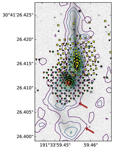
Figure 1: The HI surface density contours are plotted over the SDSS r-band image. Sky positions of the fibers in four SparsePak pointings are shown separately, with green circles, red triangles, blue stars, and yellow squares. The red cross indicates the fiber for which the spectrum is shown in Figure 2. The centers of the two galaxies and the northern tail match in r-band image and HI map. The southern tail, however, appears to have two self-gravitating clouds of cold gas (indicated by the brown arrows). These self-gravitating features can not be reproduced with test-particles in Identikit. We use the morphology of the r-band image along with the kinematics of the HI gas.

For SparsePak observations we used the bench spectrograph and the 860 lines/mm grating blazed at 30.9^∘ in order 2, obtaining a dispersion of 0.69 Å/pixel (FWHM) in the wavelength range of 6050-7000Å. We obtain a velocity resolution of $\sim$ 31 km s^-1. Our spectral coverage is less than recent and ongoing galaxy surveys such as CALIFA, and MaNGA, But our spectral resolution is higher. In the red band, the dispersion of CALIFA, and MaNGA surveys are 2.0 Å/pixel and 0.83Å/pixel, respectively. Higher spectral resolution enables us to resolve multiple emission line components, usually appearing in the central regions of galaxies where multiple gaseous components overlap.

2.2 Data Reduction

We fit one-component and two-component triple Gaussian curves on top of a line with free slope as the background (continuum) over the wavelength range 6665-6755 $\AA$ where H$\alpha$ and [N II]  emission lines appear for the Mice system. The triple Gaussian curves have free amplitudes, with centers separated by the wavelength difference between [N II][$\lambda 6548$], H$\alpha$[$\lambda 6563$], and [N II][$\lambda 6584$]. The ratio of [N II][$\lambda 6584$]/[N II][$\lambda 6548$] was fixed to the theoretical value of 2.95 (Acker et al., 1989). The signal to noise of the continuum is not high enough to fit the stellar model properly. As a result, in our analysis we did not take the underlying H$\alpha$ absorption into account. We use an F-test to decide which fit to the emission lines is favored by our data. Two-component fits are usually preferred in the central regions where the signal to noise is higher and parts of the system with different velocities are likely to overlap. Figure 4a shows fibers in which double component fits were favored. In each of these fibers, narrow and broad components are determined by their velocity dispersion. In some of the very central fibers even a two-component fit is not enough to properly model the shape of the emission line. Figure 2 shows an example of a fiber where two-component model is preferred. This fiber is marked with the red cross in Figure 1. In Figure 2b we compare the CALIFA spectrum of the exact same location on the Mice. The multiple components are clearly washed out in CALIFA data due to lower spectral resolution.

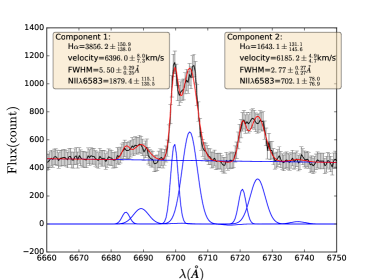
(a)

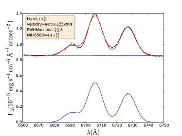
(b)

Figure 2: (a) An example of the SparsePak spectrum in one of the central fibers (indicated with the red cross in Figure 1). The black points with error bars show the spectrum data points. The solid blue curves show the fitted triple Gaussians (two components) and the the fitted background line. The red solid line shows the sum of fitted functions. One visually confirms that more that one component is required to fully describe the emission lines. In this work, we test whether two components are resolved in each fiber. (b) CALIFA spectrum from the exact same sky position. The points and solid lines are the same as (a). The lower spectral resolution of CALIFA instrument washes out the multiple components.

2.3 Shocked vs. Star Forming Regions

H$\alpha$ emission originates from ionized gas regardless of how the gas was ionized. In normal HII regions, atomic hydrogen is photo-ionized by the UV emission from O/B stars. Photoionization does not significantly affect the overall kinematics of the gas relative to old stars and the neutral gas in the vicinity. We expect the velocity obtained from H$\alpha$ emission of these photo-ionized sources to be relatively similar to the velocity of the bulk of the baryons, which is mostly governed by gravitational forces. In dynamical modeling of a galaxy merger using collisionless test particles only gravitational effects are to be considered. So, we expect H$\alpha$ kinematics of normal HII regions to be ideal for our modeling method. On the other hand, high speed stellar winds, SN remnants, and feedback from AGN produce shocks and heat up the interstellar gas. Shock-heated gas also emit H$\alpha$, but unlike photo-ionized gas, often its final velocity is significantly affected by non-gravitational processes. The kinematics obtained from H$\alpha$ emission of shocked gas can significantly disagree from that of the bulk of the baryons. Therefore, it is important to distinguish emission from the photo-ionized and shocked regions.

One way to separate the star-forming and shocked regions is to utilize the Baldwin, Phillips & Terlevich (BPT) diagnostics diagram which uses [O III]$\lambda$5007/H$\beta$, [N II]$\lambda$6583/H$\alpha$, [S II]$\lambda\lambda$6716,6731/H$\alpha$, and [O I]$\lambda$6300/H$\alpha$ flux ratios (Baldwin et al. 1981, Kewley et al. 2006). Our SparsePak observations, however, were limited to wavelength range of 6050-7000 Å and did not include H$\beta$ and [O III] emission lines. We need a different method to distinguish shocks from normal star-forming regions.

The shocked regions tend to have higher [N II]/H$\alpha$ and usually exhibit higher velocity dispersion. Rich et al. (2011) showed that the histogram of velocity dispersion of emission line components in some galaxy mergers reveals a bi-modality. The emission from star forming regions and shock heated gas appears to be responsible for the low and high velocity dispersion modes, respectively. Via further analysis of a larger sample, including interacting systems in various merger stages, Rich et al. (2014) chose a limit of $\sigma<90$ km/s for the velocity dispersion of emission lines from HII and turbulent star forming regions. The components with $\sigma>90$ km/s are, hence, considered to be emitted from low velocity shocks. On the other hand, [NII] BPT diagram suggests that when log₁₀([N II]/H$\alpha$)<-0.2, the emission is more likely to originate from star forming regions, i.e. below the dashed curve in Figure 4a of Kewley et al. (2006). Components with larger log₁₀([N II]/H$\alpha$)are from either the composite or AGN regions of [N II] BPT diagram. However, many IFU observations of extended nebular emission in galaxies have suggested that the galaxy-wide shocks are the sources of composite emission, not a mixture of AGN and star formation. (Monreal-Ibero et al., 2006; Monreal-Ibero et al., 2010; Farage et al., 2010; Rich et al., 2011, 2014, 2015) Following the argument that shocked gas has higher velocity dispersion and [N II]/H$\alpha$, we use a plot of velocity dispersion vs. log₁₀([N II]/H$\alpha$)to separate the shocked regions from normal star forming ones.

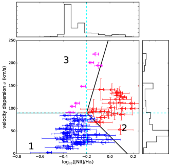
(a)

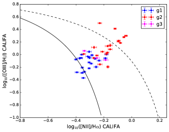
(b)

Figure 3: (a) Plot of velocity dispersion vs. log₁₀([N II]/H$\alpha$) for all components with S/N$>$5. The markers are shown as left-arrows to indicate that the values of log₁₀([N II]/H$\alpha$) are upper limit, as we did not take the underlying H$\alpha$ absorption into account in our analysis. Data points are visually classified into 3 groups. Group 1 (lower left) are taken as components emitted from normal star-forming regions. Group 2 components (right) mostly have higher log₁₀([N II]/H$\alpha$) and velocity dispersion than group 1. They are likely to have been emitted from shock-heated gas. Group 3 (upper left) components have large velocity dispersion and lower [N II]/H$\alpha$ compared to group 2, suggesting that they are the projection of multiple unresolved kinematic components. The horizontal and vertical dashed cyan lines show, respectively, the limits of $\sigma=90$ km/s and log₁₀([N II]/H$\alpha$)$=-0.2$ for separating shocks in the literature. On the top and left panels, the H$\alpha$ flux wighted histogram of these components are shown for log₁₀([N II]/H$\alpha$) and velocity dispersion, respectively. (b) [N II] BPT diagnostic diagram for fibers that preferred only one component fit in our data. For this plot CALIFA data has been used. The fibers are color-coded by their group from (a). The solid and dashed lines are from Kewley et al. (2006), dividing star forming, composite, and AGN regions. Even though most fibers are in the composite region, the location of components in groups 1 and 2 verifies that they are more likely to have been originated at star forming and shocked regions, respectively. Please note that the emission lines are taken from Sánchez et al. (2016), who have modeled the stellar continuum (underlying H$\alpha$ absorption), so they measure a slightly lower value for log₁₀([N II]/H$\alpha$).

Figure 3a shows the plot of velocity dispersion vs. log₁₀([N II]/H$\alpha$) for all kinematic components with S/N$>$5. Through visual inspection, we find that the data points are clustered into three groups. Group 1 has low [N II]/H$\alpha$ and low velocity dispersion, group 2 has high [N II]/H$\alpha$ and high velocity dispersion, and group 3 has low [N II]/H$\alpha$ and high velocity dispersion. We chose the black lines shown in Figure 3a to separate these three groups. Dashed cyan lines show $\sigma=90$ km/s (limit of shocks in Rich et al. 2014) and log₁₀([N II]/H$\alpha$)$=-0.2$ (highest value for star forming galaxies in [N II] BPT diagrams; Kewley et al. 2006). On the top and right panels, the H$\alpha$ flux wighted histogram of all components are shown for log₁₀([N II]/H$\alpha$) and velocity dispersion, respectively. As our data was not flux calibrated we estimated H$\alpha$ flux by the number of electron counts per unit exposure time. A weak bi-modality is visible in the velocity dispersion histogram, similar to systems in Rich et al. (2011, 2015); though, the peak of histogram at high velocity dispersion is weaker in our data.

In our spectral analysis we did not fit the stellar model to the spectra; instead, we used a line with free slope to model the continuum around H$\alpha$-[N II] triplet. Resultingly, we did not take the underlying H$\alpha$ absorption feature of the stellar continuum into account. This means that The H$\alpha$ equivalent width (EW) is underestimated in our analysis, and the measured [N II]/H$\alpha$ are upper limits. So, the data points in Figure 3a are shown with left arrows.

Group 1 components are taken to be the components originating from normal star forming regions. We use these components to make the H$\alpha$ velocity map for dynamical modeling. (See Figure 6a). Most of the components in this group are both below and to the left of the horizontal and vertical dashed blue lines, respectively. The smooth rotation seen across circles in Figure 6a, and their agreement with the velocity of cold gas are additional evidences that these components reveal the velocity of star forming regions.

Group 2 components are likely to be emitted from the shocked regions ,because they have both higher [N II]/H$\alpha$ and higher velocity dispersion. The spatial position of these components are shown in Figure 4b. Most of them lie on the two sides, above and below the discs near the cores of both galaxies. This is consistent with the bi-cones of shocked material seen in Figure 7 of Wild et al. (2014). Wild et al. (2014) used CALIFA data with better spectral coverage, but lower resolution compared to our data. Based on the spatial distribution of [O III]/H$\beta$ ratio and X-ray data, they argue that NGC 4676A do not host an AGN, and the source of ionization is fast outflowing shocks, probably originating from a starburst in the core. In NGC 4676B, however, they do not rule out the possibility of an AGN being the source of bi-conal structure. The overall agreement of our data with the spatial distribution of regions of high [N II]/H$\alpha$ in CALIFA, for which stellar model is taken into account, suggests that the underlying H$\alpha$ absorption does not significantly change our measurements of log₁₀([N II]/H$\alpha$).

The spatial distribution of group 3 components are shown in Figure 4c. Their high velocity dispersion and relatively low log₁₀([N II]/H$\alpha$) can be explained by projection of more than 2 components that are not resolved. Figure 4c provides additional evidence for this, showing that these components are situated in regions close to the center of the two galaxies, where it is more likely to have multiple overlapping kinematic components.

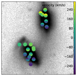
(a)

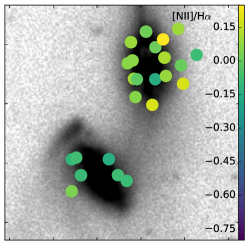
(b)

(c)

Figure 4: (a) The fibers in which two component fit is preferred over one component fit, using the F-test. The velocity of the two components are shown by the color map. The upper and lower half of each circle show the velocity of the narrow and broad components, respectively. (b) The fibers with components in group 2 of Figure 3a. The spatial distribution of these fibers is consistent with the bi-cone shocked structure seen in Wild et al. (2014), and suggests that a central process is responsible for shocks. (c) The fibers with components in group 3 of Figure 3a. These components have large velocity dispersion and low [N II]/H$\alpha$. The color of points show their velocity dispersion. They are close to the central regions where multiple gaseous component are more likely to be projected in the same line of sight. Note that the broad component in the spectrum of Figure 2 belongs to this group.

In Figure 3b, we show the distribution of components from these 3 groups on the traditional BPT diagram. Our data does not cover [O III] and H$\beta$ lines, but we can find them in CALIFA survey data. CALIFA survey has a lower spectral resolution than our data, as shown in Figure 2. We do not see multiple kinematic components in CALIFA emission lines. Also, CALIFA only covered the central regions of the two galaxies, missing the tidal tails that we covered partly. In order to inspect the components of Figure 3a in BPT diagram using CALIFA data, we select SparsePak fibers in CALIFA footprint in which one-component fit was preferred. We use the CALIFA emission line maps by Sánchez-Menguiano et al. (2016), calculate the sum of emission lines of spexels within each fiber, and measure a CALIFA line ratio for each SparsePak fiber. Figure 3b shows that most fibers are in the composite region, shown by the solid and dashed lines from Kewley et al. (2006). However, fibers in groups 1 and 2 appear to be spread along a mixing sequence from HI region to AGN. Fibers in group 1 tend to have a more HII region-like emission, while group 2 clearly indicates a harder source of ionization. This provides additional support for our method of separating shocks from star forming regions, only using velocity dispersion and log₁₀([N II]/H$\alpha$). Group 3 components are situated in the middle of the other two groups, in line with our suggestion that they could be unresolved combination of group 1 or 2 components.

Careful reader may notice that in Figure 3b some fibers in group 2 have log₁₀([N II]/H$\alpha$)<-0.2, while in Figure 3a group 2 components are defined to have a minimum value of -0.2 for log₁₀([N II]/H$\alpha$). This inconsistency is due to the fact that the model of emission line ratios of Figure 3b by Sánchez-Menguiano et al. (2016), includes stellar continuum model and takes the underlying H$\alpha$ absorption line into account. As a result, the log₁₀([N II]/H$\alpha$) at a given fiber of Figure 3a tend to be slightly smaller in Figure 3b. This is shown, more clearly, in the left panel of Figure 5. Figure 5 shows log₁₀([N II]/H$\alpha$), velocity, and velocity dispersion derived from our data vs. CALIFA data (Sánchez et al., 2016) for fibers in Figure 3b. The velocity of the two data sets agree, and the velocity dispersion measured from our data is smaller than that of CALIFA due to the better spectral resolution of our data.

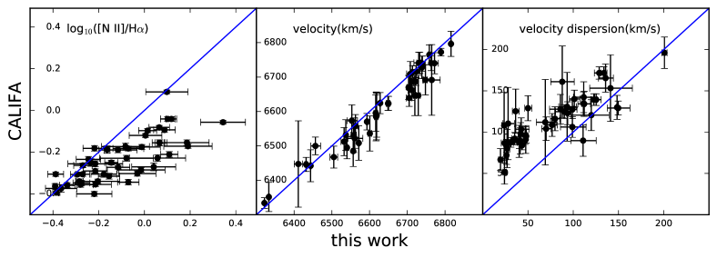
Figure 5: Plot of values of log₁₀([N II]/H$\alpha$), velocity, and velocity dispersion derived from our data vs. CALIFA data (Sánchez et al., 2016). Here we only show fibers in which one-component fit is preferred in our high resolution data. In the left panel, log₁₀([N II]/H$\alpha$) from our data is slightly higher that that of CALIFA, which is the result of the lack of stellar model in our emission line models. The velocities shown in the middle panel agree within one $\sigma$. Velocity dispersion measured in this work is generally smaller, specially for fibers with low velocity dispersion. This is due to the better spectral resolution of our data.

Using these groups, we can estimate the fraction of total H$\alpha$ flux emitted from shocked gas. To do so, we divide the sum of the H$\alpha$ flux from group 2 components to the total H$\alpha$ flux. Group 3 components can be unresolved components of both groups 1 and 2. We use [N II]/H$\alpha$$=-0.2$ limit to separate them for the purpose of estimating shocked gas fraction. We obtain a fraction of $23\pm 1\%$ of H$\alpha$ flux being emitted from shock-heated gas. The error of this fraction is obtained from the variance of shock fraction in 100 bootstrapped samples of data points in velocity dispersion vs. log₁₀([N II]/H$\alpha$) space (i.e. Figure 3a).

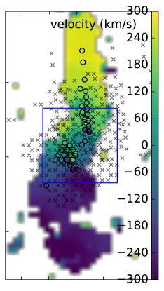
(a)

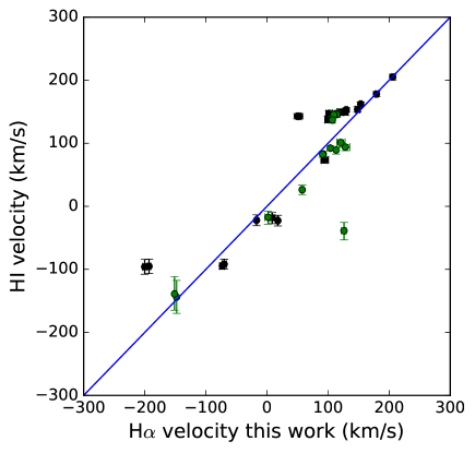
(b)

Figure 6: (a) Velocity of components in group 1 of Figure 3a, which have low velocity dispersion and low [N II]/H$\alpha$, over-plotted on the HI Velocity map. There is an agreement in the overall velocity gradient and the velocity of tidal tails. The blue box shows the zoom-in area of panels in Figure 4. (b) The velocity obtained from HI vs. group 1 H$\alpha$ emission lines at the location of corresponding fibers. Some HI and H$\alpha$ emission lines reveal two kinematic components. The black data points are for the fibers where a single component fit is preferred for both HI and H$\alpha$. The green points are for fibers in which either HI or H$\alpha$ preferred a double component fit, and we only plot the velocities of the components that better match to the other velocity tracer.

3 JVLA HI data

The kinematics of cold gas are available from radio interferometric observations of HI 21 cm emission line performed by Hibbard & van Gorkom (1996). The observations took place in May of 1991 and May of 1992 using the D and C configurations of then Very Large Array (VLA), respectively. The HI data has a spatial resolution of 20” ($\approx$ 9 kpc) and velocity resolution of 43.1 km/s. The total HI mass in the system is $7.5\times 10^{9}M_{\odot}$ (Hibbard & van Gorkom 1996; Wild et al. 2014).

In the Mice, there are a couple of self-gravitating/dissipative features in the southern tail with no counterparts in the optical r-band image. They are indicated by the brown arrows in Figure 1. After a few unsuccessful trials to reproduce these features with Identikit, we decided to use the morphology of the optical image (SDSS, r-band) along with the velocity of the HI gas, same as Privon et al. (2013).

3.1 Kinematics of H$\alpha$ vs. H I

Figure 6a shows the H$\alpha$ velocity map the mice galaxies, obtained from group 1 star forming components of Figure 3a, over-plotted on the H I velocity map. HI velocities are measured as the average of velocities of channels in the HI data cubes, weighted by flux density at each channel. In this color plots the striking agreement between the two velocity maps is evident. This agreement is especially important in the tidal tails which play the most important role in dynamical modeling, because we try to find the model that best matches the morphology and kinematics of these features.

In order to better show the agreement between velocities of star forming H$\alpha$ emission and the cold gas, in Figure 6b, we show a plot of group 1 H$\alpha$ velocities vs. HI velocities at the location of the corresponding fibers. We noticed that some HI emission lines also reveal more than one kinematic components, so similar to our procedure for H$\alpha$-[N II] triplet, we performed one- and two-component Gaussian fitting on HI 21cm emission line, and used the F-test to determine which fit is preferred. In Figure 6b, black data points show fiber in which both HI and H$\alpha$ data prefer a single component fit. The green points show places that either HI or H$\alpha$ data prefer two components, and we only show the components for which the velocities match. As can be seen in Figures 6a and 6b, in most fibers, HI and group 1 H$\alpha$ velocities match to within the error bars. The disagreement in some fibers near the center can be attributed to the low spacial resolution of HI data and the beam smearing effect.

4 Dynamical Modeling

For dynamical modeling of the Mice, we use the automated pipeline that was developed based on Identikit (Barnes & Hibbard 2009, Barnes 2011; Mortazavi et al. 2016). Identikit is a software package for modeling the initial condition of major galaxy mergers. It uses a precompiled library of N body simulations of galaxy mergers with different initial conditions. The discs are modeled by test particles. This facilitates the run of multiple discs at the same time, and improves the pace of search in the parameter space. Interactive visual matching with Identikit was used by Privon et al. (2013) to model the Mice along with 3 other systems.

The isolated galaxies consist of collisionless massive and massless test particles. massive particles are distributed in spherically symmetric fashion representing the mass of the dark matter halo, the disc, and the bulge. In these models, the luminous mass fraction, $f_{L}=(M_{d}+M_{b})/(M_{h}+M_{d}+M_{b})$ is 0.2 and the concentration parameter of the halo mass profile, $c_{h}$ is 4. The discs are represented by test particles that are initially in circular orbits. The scale length of the disc , $a_{d}$, is 1/3 of the scale radius of the dark matter halo, $a_{h}$. Barnes (2016) explored the effect of different structure parameters of the isolated galaxies on the morphology of tidal features. In this work we keep working on a single mass model for the sake of simplicity.

We use an automated matching feature that was introduced in Identikit II (Barnes, 2011). In Identikit II, the similarity between model and data is quantified with an informal measure called score. The user places small boxes in the same position as the tidal tails and bridges of the system, extended in two spatial directions and the LOS velocity direction. Identikit calculates the scores based on the number of disc test particles residing in these phase space boxes. The models that better reproduce the tidal features would place more particles in these boxes, and they would gain a better score. Identikit II has been applied with a limited range of parameters on the Mice galaxies by Barnes & Privon (2013). They inspected the models with high score visually and confirmed that they show good, or fair visual match with the HI data.

In Mortazavi et al. (2016) we described the method that we have developed for automated searching of parameter space and reconstructing the initial parameters with robust uncertainties. In this method we first put the boxes on tidal features of the galaxy merger using a semi-automated technique. The boxes are placed randomly in regions that are far enough from the center of galaxies. Boxes near the center of the galaxies, where test particles have higher number density, are always populated, and they do not put strong constraint on the initial conditions of the merger. As a result, we put the boxes over the ends of the tidal tails to enforce the similarity in the overall shape and the velocity gradient. We ignore self-gravitating features like stellar clusters or blobs of gas, because test particles in Identikit do not reproduce them. In cases where no velocity information is available (e.g. the absence of H$\alpha$ in the southern tail of the Mice), we put boxes that are only extended in spatial directions, and do not put constraint on velocity. The size of the boxes are selected to match the spatial resolution of the observation. In case of the HI data The boxes are 8 kpc wide, almost matching the spatial resolution of JVLA observation of Hibbard & van Gorkom (1996). When modeling the H$\alpha$ kinematics, the size of the boxes where set to be close to the size of SparsePak fibers (4 kpc). In places where the error in H$\alpha$ velocity measurement was larger that the extent of the box in velocity direction, we increased the size of the box proportionally. Figure 8 shows a sample of selected boxes in morphology and velocity directions.

Table 1 shows the range of encounter parameters we explored in this work. We produced a library of Identikit models with a variety of eccentricity, pericentric separation, time since first pass, velocity scaling and velocity offset. For future references we call these five parameters “external parameters". Calculating the score for each of these models, Identikit constrains viewing angle, initial orientation of discs, length scaling and position offset. We call these parameters “internal parameters". By calculating the score for all library members, we obtain a 5 dimensional score map for external parameters. Each point of this score map corresponds to a set of calculated internal parameters. The model with the maximum score is the best-fit model and the corresponding external and internal parameters are the best-fit encounter parameters.

Parameter Class	Parameter	Range Tested
orbital parameters	eccentricity	[0.80-1.10]
	pericentric distance	[0.03125-1.0000]$\times R_{vir}$
	mass ratio	1
observer dependent	time since pericenter	from first pass to second pass
parameters	viewing angle	viewed from 320 evenly distributed
		directions on a sphere
	position	set by locking the centers
	length scaling $\mathcal{L}$	set by viewing angle and locking the centers
	velocity offset	[-0.1,0.1]
	velocity scaling $\mathcal{V}$	[-0.500-+0.500]∗
initial orientation		1280 evenly distributed orientations
of discs

Table 1: Range of encounter parameters explored. The total number of parameter space points for which we calculated score is $\sim 3.2\times 10^{10}$. ^∗ The velocity (length) scaling, $\mathcal{V}$ ($\mathcal{L}$), relates the dimensionless velocity (length) in Identikit to the physical velocity (length).

The uncertainty of the best-fit parameters are calculated using a Bootstrap statistical method. Score, by itself, does not provide statistical probability as other measures of goodness of the fit like $\chi^{2}$. So, in order to estimate the uncertainty of the scores we re-do the random box positioning procedure several times (10 times in this work), and calculate the score each time. This process randomly moves the position of boxes on the tidal tails and bridges of the system. The variation in the scores for each model measures the error of the score, which eventually, translates into the uncertainty of the best-fit parameters. The models with scores that are within 1, 2, or 3 standard deviation from the best score, respectively, determine the extent of 1$\sigma$, 2$\sigma$, or 3$\sigma$ separation in the parameter space from the best-fit model.

In Mortazavi et al. (2016) we applied our modeling method on on edge-on views of hydrodynamical simulations of prograde disc-disc interactions (similar to the Mice). We evaluated the bias in the reconstructed interaction parameters comparing them to the known input parameters of the hydrodynamical simulations. We showed that when testing young stars in the simulation (representing the H$\alpha$ data), the average bias is not significant in eccentricity, $\mathrm{R_{peri}}$, and merger stage ($<1\sigma$). When testing the cold gas of the same simulation, the reconstructed physical $\mathrm{R_{peri}}$ was almost twice the correct value, but the reconstruction of eccentricity and time was only biased by less that 1$\sigma$.

4.1 Summary of Results

	fractional	physical	$e$	merger stage	physical time	$(\theta,\phi)$	NGC 4676A	NGC 4676B
	$\mathrm{R_{peri}}$	$\mathrm{R_{peri}}$		$\Delta T/T_{\textrm{first to}}$	(Myr)	degrees∘	$(i_{1},\omega_{1})$	$(i_{2},\omega_{2})$
	($\mathrm{R_{vir}}$)	(kpc)		${{}_{\textrm{second pass}}}^{*}$			degrees∘	degrees∘
H$\alpha$	$0.38\pm^{0.16}_{0.09}$	$17\pm^{12}_{6}$	$\leq 0.80\pm^{0.05}_{---}$	$0.19\pm^{0.21}_{0.01}$	$200\pm^{40}_{30}$	$(76\pm^{3}_{9},0\pm^{61}_{41})^{*}$	$(21\pm^{11}_{5},29\pm^{33}_{38})$	$(38\pm^{21}_{10},187\pm^{20}_{24})$
HI	$0.50\pm^{0.03}_{0.44}$	$24\pm^{8}_{13}$	$\leq 0.80\pm^{0.15}_{---}$	$0.14\pm^{0.70}_{0.01}$	$170\pm^{90}_{50}$	$(67\pm^{4}_{9},52\pm^{9}_{66})$	$(56\pm^{31}_{24},50\pm^{55}_{96})$	$(69\pm^{23}_{27},162\pm^{25}_{61})$

Table 2: Reconstructed parameters from modeling H$\alpha$ and HI kinematics. ^∗ The resolution of automated search in viewing angle was $\sim 11^{\circ}$ (viewdepth parameter = 3 in Identikit; see Barnes 2011). The errors reported here are from the width of distribution of viewing angles in models with high score. Note that negative azimuthal angles should be interpreted as a 360^∘ rotation. These parameters match the definitions of Privon et al. (2013) and can be compared with their values.

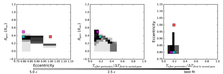
(a)

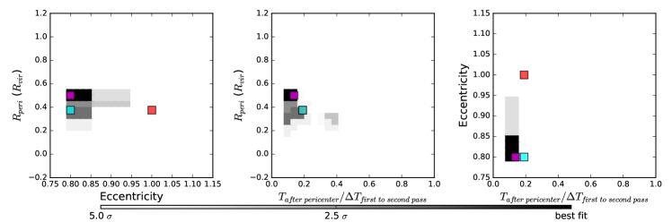
(b)

Figure 7: (a) The average score map for modeling H$\alpha$ kinematics of the Mice galaxy merger. Score map is a 5-dimensional parameter space. Here we are showing 3 slices of the score map through the best-fit parameter, across eccentricity, pericentric separation, and time since pericenter. The dark areas indicate better scores relative to light areas. The scale in the color bars is from average score at the best-fit model (the darkest) down to a score that is lower by five time the standard deviation of scores at the best-fit model (white). The best-fit model is shown with the cyan boxes, so they are located on the darkest points in all panels of (a). The magenta boxes show the the parameters of the best-fit model of HI. They are located on the darkest point of all panels in (b), which are similar slices of the average score map for modeling HI kinematics of the Mice. Cyan boxes have the same definition in (b). The red boxes in both (a) and (b) show the best-fit parameters of Privon et al. (2013) which used visual matching to HI kinematics. In the middle panels, the red box is hidden behind the cyan box, meaning that Privon et al. (2013) give the same best-fit R${}_{\textrm{peri}}$ and time as our H$\alpha$ model.

In Figure 7 one can see 3 slices of the 5 dimensional score map at the best-fit parameter point, across eccentricity, pericentric separation, and merger stage. In these plots the best-fit model can be compared with the best-fit model by Privon et al. (2013).

The best-fit parameters for H$\alpha$ and HI kinematics are presented in Table 2. The best-fit eccentricity is $\leq 0.80\pm^{0.05}_{---}$ and $\leq 0.80\pm^{0.15}_{---}$ in modeling H$\alpha$ and HI kinematics, respectively. The reason for the $\leq$ sign is that the range of eccentricities explored in this work was from 0.8 to 1.1. Obtaining the best eccentricity on the edge of our search range suggests that the reconstructed eccentricity is less than or equal to this value. The best-fit pericentric separation is $17\pm^{12}_{6}$ kpc for H$\alpha$ modeling, and is $24\pm^{8}_{13}$ kpc for HI modeling. The merger stage defined as the time since pericenter divided by the time from first passage to second passage, is $0.19\pm^{0.20}_{0.01}$ and $0.14\pm^{0.70}_{0.01}$ for H$\alpha$ and HI modelings, respectively. The best-fit time since pericenter is $200\pm^{40}_{30}$ Myrs for H$\alpha$ and $170\pm^{90}_{50}$ Myrs for HI. The best viewing angles in spherical coordinates ($\theta$, $\phi$) relative to the orbital plane is $(76^{\circ}\pm^{3^{\circ}}_{9^{\circ}},0^{\circ}\pm^{61^{\circ}}_{41^{\circ}})$ and $(67^{\circ}\pm^{4^{\circ}}_{9^{\circ}},52^{\circ}\pm^{9^{\circ}}_{66^{\circ}})$ for H$\alpha$ and HI models, respectively. For each Identikit model, we viewed the system from 320 equally separated viewing angles, so the resolution of our search in viewing angle was about $11^{\circ}$. The initial orientation $(i,\omega)$ of NGC 4676A is found to be $(21^{\circ}\pm^{11^{\circ}}_{5^{\circ}},29^{\circ}\pm^{33^{\circ}}_{38^{\circ}})$ and $(56^{\circ}\pm^{31^{\circ}}_{24^{\circ}},50^{\circ}\pm^{55^{\circ}}_{96^{\circ}})$ in modeling H$\alpha$ and HI kinematics, respectively. For initial orientation of NGC 4676B we find $(38^{\circ}\pm^{21^{\circ}}_{10^{\circ}},187^{\circ}\pm^{20^{\circ}}_{24^{\circ}})$ and $(69^{\circ}\pm^{23^{\circ}}_{27^{\circ}},162^{\circ}\pm^{25^{\circ}}_{61^{\circ}})$ for H$\alpha$ and HI modeling.

All of the reconstructed parameters for modeling HI and H$\alpha$ kinematics are consistent within $1\sigma$ uncertainty. This can be seen by comparing Figure 7 (a) and (b) in which the dark areas with high scores mostly overlap. Figure 7 also shows the model by Privon et al. (2013) which was obtained with visual matching of HI kinematics of the Mice to Identikit models and confirming the model with a fully self-consistent N-body simulation. Privon et al. (2013) only explored models with parabolic orbits (eccentricity=1). Except eccentricity, our parameters for modeling H$\alpha$ kinematics are consistent to within $1\sigma$ of the Privon et al. (2013) parameters. The parameters of our HI model are a bit further away, but still within $2\sigma$ of Privon et al. (2013). Figure 8 shows one of the best-fit models to the H$\alpha$ kinematics. This figure can be compared to Figure 5 of Privon et al. (2013).

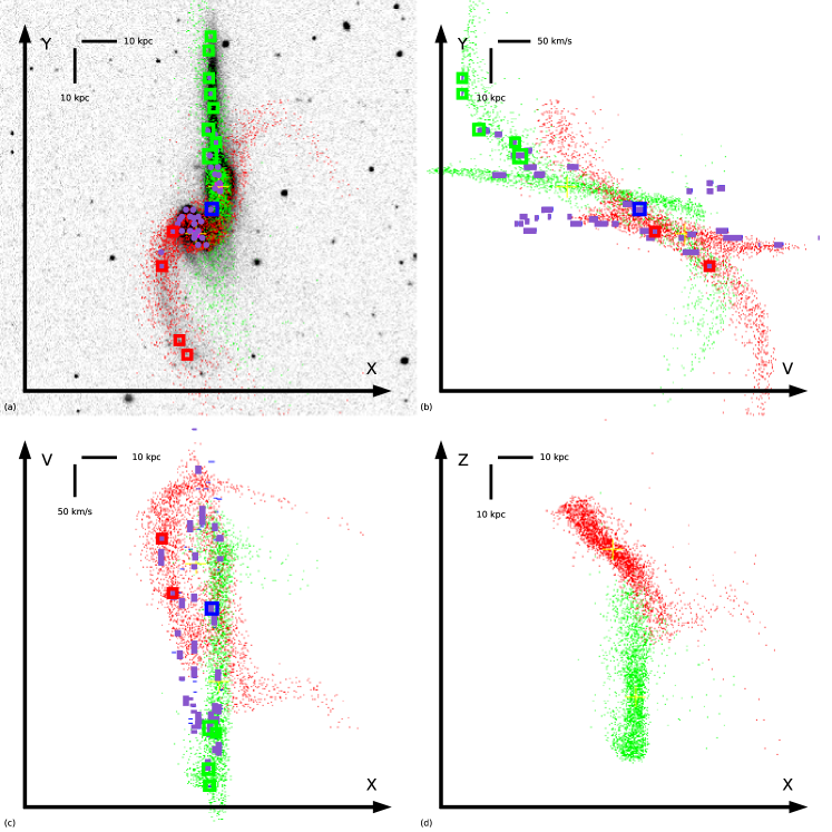
Figure 8: (a) The reconstructed Identikit model (green and red test particles) over-plotted on the SDSS r-band image of the Mice galaxies. The green, red and blue boxes indicate the phase space regions associated with NGC4676A, NGC4676B, and both discs, respectively. They are utilized by Identikit to calculate score as a measure of the goodness of the match. The purple circles show the position of SparsePak fibers used to measure the H$\alpha$ kinematics. The Identikit model reproduce the main tidal features of the Mice. However, in the model of the southern galaxy (red particles) we see an extra tidal feature in the north-west direction, which is absent in both HI and optical images. This extra feature is also present in the model presented by Privon et al. (2013).(b)(c) The line of sight velocity of the reconstructed model versus the y (x) spatial axis. The position of purple rectangles show the H$\alpha$ velocity measured at each fiber, and their extents indicate the dispersion of the H$\alpha$ emission lines. In panels (b) and (c), the position of red, green, and blue boxes along the V axis show the velocity of phase space regions, which are determined by the H$\alpha$ velocities (purple rectangles). Some boxes in panel (a) are placed where there is no H$\alpha$ velocity information (no fiber), therefore they do not have counterparts in panels (b) and (c), and are only used to constrain the morphology of the model. (d) The model viewed from the direction of the y axis in panel (a). This figure can be compared to Figure 5 of Privon et al. (2013).

5 Discussion

The peculiar morphology of the Mice has made it a curious case for dynamical modeling. There has been several attempts to model the initial conditions of this system. The reported parameters in some of these attempts are shown in Table 3. In all but one of these dynamical models the mass ratio is presumed to be 1. This assumption is made because of the similar stellar mass ratio (1.5:1, Wild et al. 2014) and the strong tidal tails in both galaxies (Toomre & Toomre 1972; Barnes 2016). We also adopt equal mass merger models in this work.

dynamical model	$\mu$	$e$	$\mathrm{R_{peri}}$	physical time since	kinematics
			(kpc)	pericenter (Myrs)
Toomre & Toomre (1972)1	1.0	0.6	…	120	H$\alpha$ only centers
Mihos et al. (1993)2	1.0	0.6	23	180	H$\alpha$ long slit
Barnes (2004)3	1.0	1.0	8.9	170	HI map∗
Privon et al. (2013)2	1.0	1.0	14.8	175	HI map∗
Holincheck et al. (2016)1	0.59$\pm$0.52	0.70$\pm$0.27	15.9$\pm$5.0	430$\pm$190	no velocity used

Table 3: Previous dynamical models of the Mice. ^∗ From Hibbard & van Gorkom (1996). ¹ Test particles with central potential. ² Collisionless self consistent simulations. ³ Hydro simulations including gas and star formation.

Time is the best-constrained encounter parameter for the Mice galaxies so far. Among the reported values in Table 3, the lowest value for time since pericenter is 120 Myr for Toomre & Toomre (1972). The largest is 430 $\pm{190}$ Myr for Holincheck et al. (2016), and the median is 175 Myr for Privon et al. (2013). Our reconstructions from HI and H$\alpha$ modeling are both consistent with the median of these models. In both of our models the Mice is found to be at a relatively early stage. The galaxies are currently at about 1/5 (1/8) of time from the first passage to the second passage for the H$\alpha$ (HI) model. Taking the uncertainty into account, both values are consistent with Privon et al. (2013) ($\approx$ 1/5). Our H$\alpha$ and HI models predict that the second passage will occur in $530\pm^{480}_{220}$ Myrs and $530\pm^{370}_{220}$ Myrs, respectively, also consistent with the model of Privon et al. (2013) for which the second passage will happen in $\approx$ 430 Myrs.

Both of our models prefer elliptical orbits, which is consistent with Toomre & Toomre (1972) and Holincheck et al. (2016). Nonetheless, in Mortazavi et al. (2016) it was shown that our modeling method underestimates the eccentricity by $\sim$0.1 in most tests on hydrodynamical merger simulations with parabolic orbits. The large error-bars in the reconstructed eccentricity in Mortazavi et al. (2016) indicate that our modeling method is not sensitive enough to eccentricity, and other constraints may be required to better constrain the initial energy of orbits in galactic encounters.

Physical pericentric distance, $\mathrm{R_{peri}}$, in our H$\alpha$ and HI models are $17\pm^{12}_{6}$ kpc and $24\pm^{8}_{13}$ kpc which are consistent with all previous reported values except that of Barnes (2004) (8.9 kpc). $\mathrm{R_{peri}}$ is hard to constrain, as its effect on morphology of tides is correlated with mass profile of isolated galaxies, i.e. disc scale-length and halo scale-radius, as well as the luminous mass fraction (Barnes, 2016). In Mortazavi et al. (2016) we showed that our method overestimates $\mathrm{R_{peri}}$ in most of the tests on hydrodynamical simulations, suggesting that our reconstruction of $\mathrm{R_{peri}}$ of the Mice is an upper limit.

Most recently, Holincheck et al. (2016) used judgment of citizen scientists (Galaxy Zoo, Lintott et al. 2010) to match the morphology of a relatively large sample of merger systems. In addition to parameters explored in this work, they varied mass ratio parameter, and they managed to present best-fit models for a relatively large sample of 62 tidally interacting galaxy pairs. For each galaxy pair $\sim 4.6\times 10^{6}$ parameter space points were rejected initially for not displaying tidal features, and $\sim$ 50,000 parameter space points were viewed and judged visually by citizen scientists. However, as seen in Table 3 , the uncertainty of their measurements are relatively large compared to the errors in this work. Lack of kinematic information in their analysis and fewer parameter space points contribute to larger error bars. In this work, we calculate the score for $3.2\times 10^{10}$ points in the parameter space elaborated in Table 1.

The strong tidal tails and the edge-on view of the Mice makes it a straight-forward case for testing a galaxy merger model. However, one may ask how common the encounter parameters of the Mice are among galaxy mergers. While the answer to this question requires modeling a larger sample of mergers, we can compare our reconstructed encounter parameters of the Mice, with the distribution of orbital parameters of dark matter halo mergers in cosmological simulations. The eccentricity of the Mice found in this work ($e\leq 0.80$), is lower than the most frequent eccentricity ($e=1.0$) among dark matter halo mergers (e.g. see Figure 11 of Benson 2005 and Figure 6 of Khochfar & Burkert 2006). Parabolic ($e=1$) orbits have zero total mechanical energy, and are expected to be seen if the protogalaxies are initially at rest and far from each other. The uncommonly low eccentricity we found may be due to a bias in our modeling method. On the other hand, it may indicate that orbits of interacting galaxies decay earlier than the dark matter halos they live in. The pericentric separation found for the Mice ($0.38\pm^{0.16}_{0.09}\ \mathrm{R_{vir}}$ and $0.50\pm^{0.03}_{0.44}\ \mathrm{R_{vir}}$ for H$\alpha$ and HI, respectively) are both uncertain. They both fall into the most common values in the distribution of $\mathrm{R_{peri}}$s in dark matter halo mergers of the Millennium cosmological simulation (see Figure 4 of Khochfar & Burkert 2006). A sanity check for this answer is to calculate the period for this elliptical orbit to see if it is longer than the Hubble time. Otherwise, one may ask why the galaxies did not merge during the previous pericenter. Assuming that the mass of the dark matter halo of the larger partner is $10^{11}-10^{12}M_{\odot}$ the period of the orbit will be 10-3 Gyrs. This is less than the age of the Universe and suggests that the orbit has become bound due to recent processes in the last 3-10 Gyrs, e.g. recent mass growth due to minor mergers.

Merger induced star formation rate (SFR) is affected by the encounter parameters in hydrodynamical simulations. Cox et al. (2008) show that mergers with larger pericentric distance induce starbursts at later times. Moreover, the relative inclination of the discs with respect to orbital plane correlates with the total amount of merger induced star formations (also see Snyder et al. 2011). On the other hand, the star formation in these simulations depends on presumptions about sub-grid physics, which are the physical processes that happen in scales smaller than the resolution of the simulation. Even the most recent simulations of galaxy formation do not yet resolve particles at scales smaller than stars. To implement star formation, most current simulations assume a density threshold above which stars are formed. The exact value of this threshold is different in different simulations and varies with the resolution of the hydrodynamical simulation (e.g. see Brooks & Teyssier 2015), and they are usually calibrated to reproduce the Kennicutt-Schmidt relationship between gas mass surface density and star formation rate (Kennicutt, 1998). Barnes (2004) proposed a shock-induced star formation recipe in order to reproduce extended merger induced star formation observed in tidal tails of interacting galaxies (e.g. see de Grijs et al. 2003). In addition to sub-grid star formation recipe, the model for feedback from SNe, stellar winds, and AGN adds to the complications of star formation model in hydrodynamical simulations (e.g. see Cox et al. 2006; Oppenheimer et al. 2010). Finding independent constraints on star formation history in galaxy mergers improves our understanding of the sub-grid physics in hydrodynamical simulations.

Our estimate of the merger stage and other encounter parameters of the Mice is independent of star formation rate. It only depends on the dynamics of tidal features. As a result, by looking at a “Mice-like" simulation of a galaxy merger with the same encounter parameters and at the same merger stage that we found in this work, we can put an independent constraint on the sub-grid physics of merger induced star formation. To do so, we can compare the total enhancement of star formation in the hydrodynamical simulation to the measured star formation in the Mice. Unfortunately, our data is not flux calibrated and we can not use it to estimate current star formation rate in the Mice galaxies. On the other hand, other measurements of the SFR in the Mice is uncertain and varies based on the observed star formation indicator. Wild et al. (2014) provide different star formation measurements for the Mice combining CALIFA IFU spectroscopy with other archival data. In particular, the SFR derived from ionized gas recombination lines (H$\alpha$ and H$\beta$) is significantly higher than the one derived from modeling the stellar continuum. While the difference may be an indicator of very recent star formation, in §2.3 we showed that about 23% of the H$\alpha$ line emission arises from sources other than photoionization. In addition, large amounts of dust attenuation, particularly at the centers of the galaxies, introduce large uncertainties in star formation rate measurements. The edge-on view of the discs may have played a role in worsening this problem. However, this works demonstrates that improvements in the measurement of star formation and dynamical merger stage of the Mice (or any other merger system) provides a powerful tool for testing sub-grid physics in hydrodynamical simulations.

5.1 Summary

In this work we modeled the initial conditions of the Mice galaxy merger system, utilizing an automated method based on Identikit software package. We observed the Mice with the SparsePak IFU on the WIYN telescope at KPNO, considered one- and two-component emission lines, and separated the emission from photo-ionized regions and shocked regions using a plot of [N II]/H$\alpha$ vs. velocity dispersion.

We used the kinematics of both photo-ionized gas (H$\alpha$) and cold gas (HI) to compare the effect of using different kinematic tracers. We found consistent results for the two kinematic tracers. They are also consistent with previous models for the Mice, particularly that of Privon et al. (2013). This work suggests that while kinematic information on tidal features is still needed, our automated method of dynamical modeling is applicable to some major galaxy merger systems using both HI and H$\alpha$ velocity information. We can use data from IFU surveys (e.g. MaNGA, SAMI, etc. ) and high resolution HI surveys (e.g. MeerKAT) to model the dynamics of major galaxy mergers. Though, one should be cautious that in some mergers systems gas does not follow stars on large scales due to dissipative processes like ram pressure striping. Dynamical reconstruction of merger stage can put independent constraints on the sub-grid physics of star formation in hydrodynamical simulations of galaxies. At this point, this is not possible for the Mice system, mostly because of the large uncertainty in star formation rate measurements.

References

- Abell et al. (2009) Abell P. A., et al., 2009, arXiv.org, p. arXiv:0912.0201
- Acker et al. (1989) Acker A., Köppen J., Samland M., Stenholm B., 1989, The Messenger, 58, 44
- Baldwin et al. (1981) Baldwin J. A., Phillips M. M., Terlevich R., 1981, Astronomical Society of the Pacific, 93, 5
- Barnes (2004) Barnes J. E., 2004, Monthly Notices of the Royal Astronomical Society, 350, 798
- Barnes (2011) Barnes J. E., 2011, Monthly Notices of the Royal Astronomical Society, 413, 2860
- Barnes (2016) Barnes J. E., 2016, Monthly Notices of the Royal Astronomical Society, 455, 1957
- Barnes & Hernquist (1996) Barnes J. E., Hernquist L., 1996, Astrophysical Journal v.471, 471, 115
- Barnes & Hibbard (2009) Barnes J. E., Hibbard J. E., 2009, The Astronomical Journal, 137, 3071
- Barnes & Privon (2013) Barnes J. E., Privon G. C., 2013, Galaxy Mergers in an Evolving Universe, 477, 89
- Benson (2005) Benson A. J., 2005, Monthly Notices of the Royal Astronomical Society, 358, 551
- Bershady et al. (2004) Bershady M. A., Andersen D. R., Harker J., Ramsey L. W., Verheijen M. A. W., 2004, Publications of the Astronomical Society of the Pacific, 116, 565
- Bois et al. (2011) Bois M., et al., 2011, Monthly Notices of the Royal Astronomical Society, 416, 1654
- Borne & Richstone (1991) Borne K. D., Richstone D. O., 1991, Astrophysical Journal, 369, 111
- Brooks & Teyssier (2015) Brooks A., Teyssier M., 2015, American Astronomical Society Meeting Abstracts, 225,
- Bundy et al. (2015) Bundy K., et al., 2015, The Astrophysical Journal, 798, 7
- Cox et al. (2006) Cox T. J., Jonsson P., Primack J. R., Somerville R. S., 2006, Monthly Notices of the Royal Astronomical Society, 373, 1013
- Cox et al. (2008) Cox T. J., Jonsson P., Somerville R. S., Primack J. R., Dekel A., 2008, Monthly Notices of the Royal Astronomical Society, 384, 386
- Croom et al. (2012) Croom S. M., et al., 2012, Monthly Notices of the Royal Astronomical Society, 421, 872
- Dubinski et al. (1995) Dubinski J., Mihos J. C., Hernquist L., 1995, arXiv.org, pp 576–
- Farage et al. (2010) Farage C. L., McGregor P. J., Dopita M. A., Bicknell G. V., 2010, The Astrophysical Journal, 724, 267
- Hibbard & Mihos (1995) Hibbard J. E., Mihos J. C., 1995, Astronomical Journal v.110, 110, 140
- Hibbard & van Gorkom (1996) Hibbard J. E., van Gorkom J. H., 1996, The Astronomical Journal, 111, 655
- Hibbard et al. (1994) Hibbard J. E., Guhathakurta P., van Gorkom J. H., Schweizer F., 1994, The Astronomical Journal, 107, 67
- Holincheck et al. (2016) Holincheck A. J., et al., 2016, Monthly Notices of the Royal Astronomical Society, 459, 720
- Jog & Solomon (1992) Jog C. J., Solomon P. M., 1992, The Astrophysical Journal, 387, 152
- Kennicutt (1998) Kennicutt R. C. J., 1998, Annual Review of Astronomy and Astrophysics, 36, 189
- Kewley et al. (2006) Kewley L. J., Geller M. J., Barton E. J., 2006, The Astronomical Journal, 131, 2004
- Khochfar & Burkert (2006) Khochfar S., Burkert A., 2006, Astronomy and Astrophysics, 445, 403
- Lintott et al. (2010) Lintott C., et al., 2010, Monthly Notices of the Royal Astronomical Society, 410, 166
- Mihos & Hernquist (1996) Mihos J. C., Hernquist L., 1996, Astrophysical Journal v.464, 464, 641
- Mihos et al. (1993) Mihos J. C., Bothun G. D., Richstone D. O., 1993, Astrophysical Journal v.418, 418, 82
- Monreal-Ibero et al. (2006) Monreal-Ibero A., Arribas S., Colina L., 2006, The Astrophysical Journal, 637, 138
- Monreal-Ibero et al. (2010) Monreal-Ibero A., V\’\ilchez J. M., Walsh J. R., Muñoz-Tuñón C., 2010, Astronomy and Astrophysics, 517, A27
- Mortazavi et al. (2016) Mortazavi S. A., Lotz J. M., Barnes J. E., Snyder G. F., 2016, Monthly Notices of the Royal Astronomical Society, 455, 3058
- Naab et al. (2014) Naab T., et al., 2014, Monthly Notices of the Royal Astronomical Society, 444, 3357
- Oppenheimer et al. (2010) Oppenheimer B. D., Davé R., Kereš D., Fardal M., Katz N., Kollmeier J. A., Weinberg D. H., 2010, Monthly Notices of the Royal Astronomical Society, 406, 2325
- Privon et al. (2013) Privon G. C., Barnes J. E., Evans A. S., Hibbard J. E., Yun M. S., Mazzarella J. M., Armus L., Surace J., 2013, The Astrophysical Journal, 771, 120
- Rich et al. (2011) Rich J. A., Kewley L. J., Dopita M. A., 2011, The Astrophysical Journal, 734, 87
- Rich et al. (2014) Rich J. A., Kewley L. J., Dopita M. A., 2014, The Astrophysical Journal, 781, L12
- Rich et al. (2015) Rich J. A., Kewley L. J., Dopita M. A., 2015, The Astrophysical Journal Supplement Series, 221, 28
- Sánchez-Menguiano et al. (2016) Sánchez-Menguiano L., et al., 2016, arXiv.org, p. arXiv:1610.00440
- Sánchez et al. (2012) Sánchez S. F., et al., 2012, Astronomy and Astrophysics, 538, A8
- Sánchez et al. (2016) Sánchez S. F., et al., 2016, Astronomy & Astrophysics, 594, A36
- Shamir et al. (2013) Shamir L., Holincheck A., Wallin J., 2013, Astronomy and Computing, 2, 67
- Snyder et al. (2011) Snyder G. F., Cox T. J., Hayward C. C., Hernquist L., Jonsson P., 2011, The Astrophysical Journal, 741, 77
- Springel & White (1999) Springel V., White S. D. M., 1999, Monthly Notices of the Royal Astronomical Society, 307, 162
- Toomre & Toomre (1972) Toomre A., Toomre J., 1972, Astrophysical Journal, 178, 623
- Towns et al. (2014) Towns J., et al., 2014, Computing in Science & Engineering, 16, 62
- Wild et al. (2014) Wild V., et al., 2014, Astronomy and Astrophysics, 567, A132
- York et al. (2000) York D. G., et al., 2000, The Astronomical Journal, 120, 1579
- de Grijs et al. (2003) de Grijs R., Lee J. T., Clemencia Mora Herrera M., Fritze-v Alvensleben U., Anders P., 2003, New Astronomy, 8, 155