The distribution of stars around the Milky Way’s central black hole:
II. Diffuse light from sub-giants and dwarfs

Abstract

Context. This is the second of three papers that search for the predicted stellar cusp around the Milky Way’s central black hole, Sagittarius A*, with new data and methods.

Aims. We aim to infer the distribution of the faintest stellar population currently accessible through observations around Sagittarius A*.

Methods. We used adaptive optics assisted high angular resolution images obtained with the NACO instrument at the ESO VLT. Through optimised PSF fitting we removed the light from all detected stars above a given magnitude limit. Subsequently we analysed the remaining, diffuse light density. Systematic uncertainties were constrained by the use of data from different observing epochs and obtained with different filters. We show that it is necessary to correct for the diffuse emission from the mini-spiral, which would otherwise lead to a systematically biased light density profile. We used a Paschen $\alpha$ map obtained with the Hubble Space Telescope for this purpose.

Results. The azimuthally averaged diffuse surface light density profile within a projected distance of $R\lesssim 0.5$ pc from Sagittarius A* can be described consistently by a single power law with an exponent of $\Gamma=0.26\pm 0.02_{stat}\pm 0.05_{sys}$, similar to what has been found for the surface number density of faint stars in Paper I.

Conclusions. The analysed diffuse light arises from sub-giant and main-sequence stars with $K_{S}\approx 19-22$ with masses of $0.8-1.5$ M_⊙. These stars can be old enough to be dynamically relaxed. The observed power-law profile and its slope are consistent with the existence of a relaxed stellar cusp around the Milky Way’s central black hole. We find that a Nuker law provides an adequate description of the nuclear cluster’s intrinsic shape (assuming spherical symmetry). The 3D power-law slope near Sgr A* is $\gamma=1.13\pm 0.03_{model}\pm 0.05_{sys}$. The stellar density decreases more steeply beyond a break radius of about 3 pc, which corresponds roughly to the radius of influence of the massive black hole. At a distance of 0.01 pc from the black hole, we estimate a stellar mass density of $2.6\pm 0.3\times 10^{7}$ M_⊙ pc^-3 and a total enclosed stellar mass of $180\pm 30$  M_⊙. These estimates assume a constant mass-to-light ratio and do not take stellar remnants into account. The fact that a flat projected surface density is observed for old giants at projected distances $R\lesssim 0.3$ pc implies that some mechanism may have altered their appearance or distribution.

1 Introduction

The existence of power-law stellar density cusps in dynamically relaxed clusters around massive black holes (BHs) is a fundamental prediction of theoretical stellar dynamics. The problem of a stationary stellar density profile around a massive, star-accreting BH was first analysed by Peebles (1972), followed by Frank & Rees (1976), Lightman & Shapiro (1977), and Bahcall & Wolf (1976). Eight years before Peebles (1972), Gurevich (1964) had obtained an analogous solution for the distribution of electrons in the vicinity of a positively charged Coulomb centre. Since then, many authors have worked on this problem with a broad variety of methods and have come to similar conclusions (see, e.g. Amaro-Seoane et al. 2004; Alexander 2005; Merritt 2006, and references therein).

The in principle best-suited environment where we can test the presence of such a cusp is the nuclear star cluster around the massive black hole at the centre of the Milky Way (e.g. Genzel et al. 2010; Schödel et al. 2014b). Unfortunately, the observations have been limited to the red clump (RC) stars and brighter giants so far. The density profile of these stars appears to suggest the absence of a stellar cusp (Buchholz et al. 2009; Do et al. 2009; Bartko et al. 2010). However, these stars only represent a small fraction of the old stars in the nuclear cluster. It has been proposed that stellar collisions removed their envelopes in the innermost, densest regions of the cusp, which would render them invisible (see, e.g. Alexander 1999; Dale et al. 2009), but this cannot fully explain the observations. Stars that formed less than a few Gyr ago would not be dynamically relaxed and could thus display a core structure (Aharon & Perets 2015), but the star counts are dominated by RC stars, which are typically older than a few Gyr. Also, the star formation history of the central parsec shows that at around 80% of the stars formed more than 5 Gyr ago (Pfuhl et al. 2011). Another possibility, that has been recently put forward, is that they interacted in the past with (a) fragmenting gaseous disc(s), which is an efficient way to get rid of their envelopes (Amaro-Seoane & Chen 2014). The results of Kieffer & Bogdanović (2016) partially reproduce the findings of Amaro-Seoane & Chen (2014), but they focused on more compact stars, typically red clump stars, and find that more hits are required to strip off the envelope of the star, as stated in the work of Amaro-Seoane & Chen (2014).

The fact that we are dealing with a fundamental problem of stellar dynamics, the ambiguity of the observational data and their interpretation, as well as the implications of stellar cusps for the frequency of Extreme-Mass Ratio Inspirals (EMRIs, see Amaro-Seoane et al. 2007 and the review Amaro-Seoane 2012 and references therein), and thus on the detection rate of sources of gravitational radiation (Hopman & Alexander 2005), have urged us to revisit this topic. In particular, the L3 mission of the European Space Agency has been approved to be devoted to low frequency gravitational wave astronomy, with EMRIs being an important class of potential sources. The mission implementing this science will follow the Laser Interferometer Space Antenna (LISA) mission concept (Amaro-Seoane et al. 2012, 2013) or a similar one, like the Chinese Taiji concept (Gong et al. 2015)..

This is the second one of a series of papers addressing the distribution of stars around Sagittarius A* (Sgr A*). They are closely related and use the same data, but focus on different methods and stellar populations. In this work we use the diffuse light density, while in our first paper (Gallego-Cano et al. arXiv:1701.03816, from now on referred to as Paper I), we analyse the star counts from the brighter, resolved stellar population. We also refer the interested reader to the more detailed introduction of Paper I for more details about the history and the current state of the investigation of the stellar cusp at the centre of the Milky Way.

Our primary goal is to find the predicted stellar cusp of the nuclear stellar cluster (NSC) around Sgr A*. To reach this aim, we push the boundaries of observational evidence by reaching towards fainter magnitudes and thus accessing a more representative sample of stars in the nuclear cluster. In Paper I, we show how we use stacking and improved analysis methods to provide acceptably complete star counts for stars about one magitude fainter than what has been done up to now. These stars, of observed magnitudes $K_{s}\approx 18$ at the distance and extinction of the Galactic Centre (GC), could be sub-giant stars, with masses of $1-2\,M_{\odot}$, and potentially be old enough to be dynamically relaxed. Indeed, their distribution inside of a projected distance of $R\lesssim 1.0$ pc can be approximated well by a single power-law with a slope of $\Gamma=0.47\pm 0.07$. This finding is consistent with the existence of a stellar cusp of old stars around Sgr A*, as we discuss in Paper I. Here, we focus on the diffuse stellar light density around Sgr A*, which provides us with information on even fainter stars.

2 Data reduction and analysis

2.1 Basic reduction

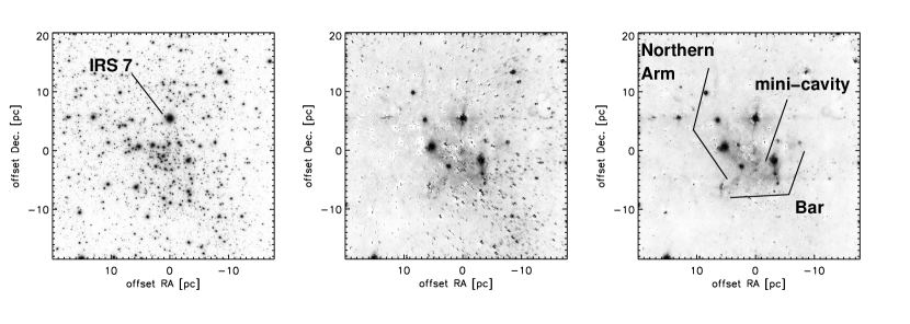
Figure 1: Source subtraction. Left: Deep $K_{S}$-band mosaic (see Paper I). Middle: Deep $K_{S}$-band mosaic with all detected stars subtracted, using a single, constant PSF, for the entire field. Right: Deep $K_{S}$-band mosaic with all detected stars subtracted, using a locally extracted PSF kernel merged with a constant halo, that is estimated from IRS 7. Typical features of the mini-spiral of gas are indicated. Logarithmic colour scale in all images, with the same scale used in the middle and right panels. North is up and east is to the left.

We use the same $H$ and $K_{S}$-band data obtained with the S27 camera of NACO/VLT that are used in Paper I and, additionally, $K_{S}$-band NACO/VLT S13 camera data from 4 May/12 June/13 August 2011, 4 May/9 August/12 September 2012, and 29 March/14 May 2013. We follow the same data reduction steps. The S13 images were stacked to provide a deep image, as done with the S27 images in Paper I. In addition, we use the calibrated HST/NICMOS 3 image of the emission from gas at $1.87\,\mu$m, that was presented by Dong et al. (2011). We also make use of NACO/VLT S27 Brackett-$\gamma$ (Br$\gamma$) narrow band (NB) observations, obtained on 5 August 2009, with a detector integration time ($DIT$) of 15 s, 3 averaged readouts per exposure ($NDIT=3$), and 45 dither positions ($N=45$). Data reduction was standard, as described in Paper I, including rebinning to a finer pixel scale by a factor of 2. Finally, we use the intermediate-band (IB) filter imaging data at $2.27\,\mu$m described in Table 1 of Buchholz et al. (2009).

2.2 Source subtraction

Subtraction of detected stars is a critical step when estimating the diffuse light. A particular challenge in AO observations is the presence of the large seeing halo (FWHM on the order $1"$) around the near-diffraction limited core of the PSFs. The dynamic range of the detected stars comprises $>$10 magnitudes, from the brightest star, GCIRS 7 with $K_{S}\approx 7$ to the faintest detectable stars with $K{s}\approx 19$ (see Paper I). Many of the brightest stars ($K_{S}=9-11$) are young, massive stars concentrated in the IRS 16, IRS 1, IRS 33, or IRS 13 complexes in the central 0.5 pc (e.g. Genzel et al. 2003; Lu et al. 2005, 2009; Paumard et al. 2006). They must be carefully subtracted to avoid a bias in the surface light density. In addition, the PSF changes across the field due to anisoplanatic effects, and the variable source density and extinction mean that the faint wings of the PSFs cannot be estimated with similar signal-to-noise in all parts of the field because there is not a homogeneous density of bright, isolated stars.

As explained in Paper I, we extracted the PSFs on overlapping sub-fields, smaller than the isoplanatic angle. In each of these sub-fields we used about ten isolated stars – the brightest ones possible – to estimate the PSF core. We then fitted the PSF halo determined from the brightest star in the field, GCIRS 7, to the cores. Schödel et al. (2010) have shown for NACO AO GC data that the variation of the PSF halo is rather negligible, which means that with the chosen approach we can reach a photometric accuracy of a few percent across the entire field. Subsequently, point sources are detected and subtracted. Since the detection of occasional spurious sources is no source of concern for this work, we chose a more aggressive approach than in Paper I, setting the StarFinder parameters $min\_correlation=0.70$ and $deblend=1$ for all images (except if stated explicitly otherwise). We note that even with these settings the detection completeness falls below 50% for sources fainter than about $K_{S}=18.5$ in the centralmost arcseconds. We note that we only perform point-source fitting and subtraction, but do not model the diffuse background with StarFinder, that is, the keywords $BACK\_BOX$ and $ESTIMATE\_BG$ are set to zero.

In order to have an extinction map that covers even the large area of the wide field observations from May 2011, we created an extinction map from HAWK-I $H$ and $K_{S}$ speckle holography-reduced FASTPHOT observations of the central square arcminutes (Nogueras-Lara et al., in prep.). We used the extinction law of Schödel et al. (2010) ($A_{\lambda}\propto\lambda^{-2.2}$), assumed a constant intrinsic colour of $(H-K_{S})_{0}=0.1$ for all the stars, and used the mean of the 20 nearest stars for each pixel. This results in an extinction map with a variable angular resolution of roughly $2"$. The results presented in this paper are not sensitive in any significant way on the variation in these assumptions within their uncertainties. In particular, changing the exponent of the extinction law to other plausible values (e.g. $2.0$, see Nishiyama et al. 2009) will have an impact on any of the parameters of interest that is a factor of a few smaller than other sources of uncertainties that will be discussed here.

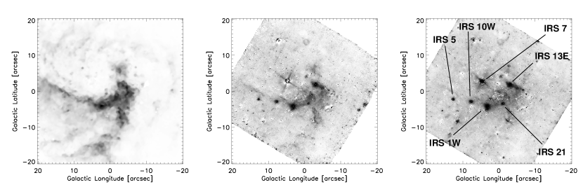
Figure 2: Left: HST NIC3 point-source-subtracted Pa $\alpha$ image of the GC. Middle: VLT NACO point-source-subtracted Br-$\gamma$ image. Right: VLT NACO point-source-subtracted $K_{S}$ image. Some prominent point-like emission sources (see text) are labelled.

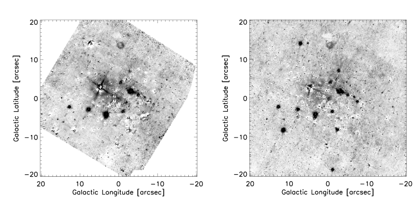
Figure 3: Left: Point-source-subtracted Br-$\gamma$ image minus scaled Pa $\alpha$ image. Right: Point-source-subtracted $K_{S}$ wide field image minus scaled Pa $\alpha$ image.

We demonstrate the result of this strategy in Fig. 1. There, we show the mosaic of the deep $K_{S}$ image (see Paper  I), and the same field after subtraction with a single, constant PSF, and after subtraction with a variable PSF, composed of a local core plus a global halo. As can be seen, using a single, constant PSF leads to variable artefacts associated with the stellar sources across the field (see also Schödel 2010). Also, when the wings of the PSF are not determined with high signal-to-noise, then the diffuse emission is dominated by flux from the seeing halos around bright stars.

With the variable core plus halo PSF (determined from the brightest star IRS 7, right panel), the residuals around bright stars are strongly suppressed and any remaining residuals are largely constant across the field, as can be seen in the right panel of Fig. 1. These remaining residuals are typical for PSF subtraction with an empirical PSF when the PSF is not fully constant across the field: Since several stars have to be used to derive a median PSF, their slightly different PSFs will result in a slightly too broad median PSF. This leads to the typical and inevitable artefacts in the form of core-excesses with surrounding negativities that can be seen around bright stars. Nevertheless, as can be seen, the residuals around the bright stars have been strongly suppressed with our method. The only exception is GCIRS 7, which is extremely bright (a few magnitudes brighter than any other source in the field). The filamentary structure of the so-called mini-spiral (see Genzel et al. 2010, and references therein) becomes apparent, with features such as the northern arm, the bar, or the mini-cavity clearly visible. We provide further detailed tests of our methodology in Appendix A.

2.3 Subtraction of mini-spiral emission

As we can see in the right panels of Figs. 1 and 2, diffuse emission from the so-called mini-spiral (see., e.g. Genzel et al. 2010) contributes significantly to the diffuse emission within about 0.5 pc ($\sim$$12"$ for a GC distance of 8 kpc) of Sgr A*, even in broad band images. We therefore have to correct for it before we will be able to estimate the diffuse emission arising from unresolved stellar sources. At the wavelengths considered, the emission can arise from hydrogen and helium lines (e.g. HI at $2.17$, $1.64$ or $1.74\,\mu$m, HeI at $1.70$, $2.06$, or $2.11\,\mu$m), but some contribution from hot and warm dust is also plausible. In Fig. 2 we show the mini-spiral as seen in the Paschen $\alpha$ line with NIC3/HST and in the Brackett$\gamma$ line as well as in $K_{S}$ with NACO/VLT, respectively. The Pa $\alpha$ image is from the survey by Wang et al. (2010) and Dong et al. (2011).

Since we will use the HST image as a reference for gas emission, we aligned all our images via a first order polynomial transform with the HST image. The positions of detected stars were used to calculate the transformation parameters with IDL POLYWARP and the images were then aligned using IDL POLY_2D. The pixel scale of the resulting images is set to the one of the HST image ($0.101"$ per pixel).

As can be seen in Fig 2, the Pa $\alpha$ image traces the gas emission very clearly (with the exception of a few Pa $\alpha$ excess sources, see Dong et al. 2012) and the $K_{S}$ and Br $\gamma$ images of the diffuse emission trace the same structures of the mini-spiral. Some differences are given by residuals around bright stars, by some residual emission associated with the brightest star, GCIRS 7, by hot dust emission around the probable bow-shock sources IRS 21, IRS 10W, IRS 5, and IRS 1W, and by enhanced emission in and around the IRS 13E complex, probably from a higher gas temperature. We mark some of these sources and areas in Fig. 2 and will mask them when deriving scaling factors for gas subtraction and when computing the brightness of diffuse stellar light in the following sections.

Figure 3 shows the point source-subtracted Br $\gamma$ and $K_{S}$ images after subtraction of the scaled Pa $\alpha$ image. The scale factor was assumed constant and estimated by eye. All images were corrected for differential extinction. We also determined the scaling factor in a numerical way fitting the azimuthally averaged surface brightness distribution with a least $\chi^{2}$ fit with a linear combination of the scaled azimuthally averaged surface brightness distribution of the Pa $\alpha$ emission plus a simple power-law diffuse light density distribution centred on Sgr A*.

$$\Sigma(R)=\Sigma_{0}*(R/R_{0})^{-\Gamma}+\beta Pa\,\alpha,$$ (1)

where $\Sigma_{0}$ is the surface flux density at a the projected distance $R_{0}=0.5$ pc, $\Gamma$ is the power-law index, Pa $\alpha$ is the Paschen $\alpha$ SB, and $\beta$ the scaling factor for the latter. There are three free parameters, $\Sigma_{0}$, $\Gamma$, and $\beta$ . We limited the estimation of $\beta$ to the region $R\leq 0.5$ pc, where the gas emission is strongest. Varying this value up to $R=1.5$ pc does not have any significant effects on the SB profiles, but some negativities can then appear after minispiral subtraction in the images because the fit is dominated by regions at large $R$ with low gas SB, where the excitation conditions of the gas may also be different (greater distance from the hot stars near Sgr A*). The resulting best-fit factor was close to our by-eye estimate.

We considered fitting the azimuthally averaged surface brightnesses as marginally more reliable than directly fitting the images because the azimuthal average will suppress noise from the data acquisition and reduction process, from the point-source subtraction, and from potential variations of the gas temperature. Nevertheless, we also tested direct fitting of the models to the images and obtained the same results within the formal uncertainties of the fits. As can be seen in Fig. 3, most of the emission from the gas and dust in the mini-spiral can be effectively removed by this simple procedure. From our by-eye fit we estimated an uncertainty of $10\%$ for the best scale factor, while its uncertainty from the least $\chi^{2}$ fits is $<5\%$. This uncertainty has a negligible effect on the parameters we are interested in, in particular the slope of the power-law surface density. For all images and wavelengths used in the following we applied the numerical procedure to estimate the scaling factor for the subtraction of the diffuse gas emission.

An alternative way of subtracting the mini-spiral emission may be by using the intrinsic line ratio of $Br\,\gamma/Pa\,\alpha$. However, this is not practical in our case because most of our data are broad-band observations and include additional lines, for example from the $2.058\,\mu$m He I line in the $K_{S}$-band. Also, in the case of the $Br\,\gamma$ image, no accurate calibration was possible because no zero point observations were taken at the time of the observation and the sky conditions were not photometric.

Finally, NIR emission from the mini-spiral may also arise, at least partially, from hot dust, in particular near young, massive stars, such as the IRS 13 region or the putative bow-shock sources IRS 21, IRS 1W, etc. (see, e.g. Eckart et al. 2004; Fritz et al. 2010; Sanchez-Bermudez et al. 2014). This is plausible because the morphology of the emission from warm/hot dust in the mini-spiral region resembles closely the one observed in line emission (compare, e.g. the images of the mini-spiral seen through different filters in Mužić et al. 2007; Wang et al. 2010; Genzel et al. 2010; Lau et al. 2013). We did some experiments in this respect, with point-source subtracted $8.6\,\mu$m and $3.8\,\mu$m imaging data (Schödel et al. 2011) and found dust temperatures on the order of 250-350 K. This is hotter than in the SOFIA observations analysed by Lau et al. (2013) and is probably related to us using data of considerably higher angular resolution and considerably shorter wavelengths or to the fact that the $8.6\,\mu$m image may be dominated by emission from PAHs.

When we correct the measured diffuse SB profile in $K_{s}$ with our dust emission map, we get roughly similar results than with the HST Pa $\alpha$ image. However, the quality of the correction is considerably worse because (a) the HST data provide much cleaner measurements of the diffuse gas emission, (b) the FOV of our $8.6\,\mu$m and $3.8\,\mu$m imaging data is smaller than the one of the HST images, (c) point sources must first be subtracted from the NIR/MIR images, which introduces additional systematic errors, and (d) further systematics are introduced by the very challenging determination of the variable sky background in the MIR observations (it is impossible to chop into an emission-free region inside the GC). The fundamental assumption in our work is that the non-stellar diffuse emission can be obtained from the HST Paschen $\alpha$ image through applying a constant scaling factor. As long as this assumption is approximately valid, it does not really matter whether we are dealing with line emission and/or dust emission. A study of variable line-emission and variable gas or dust temperature in the mini-spiral is beyond the scope of this paper. As we show below, our method to remove the non-stellar diffuse emission appears to work very well and provides consistent results across many filters. We therefore believe our method to be solid.

3 The surface density of faint stars in the GC

In this section we explore the surface brightness (SB) profile of the diffuse stellar light in observations taken with different cameras and filters, as well as at different epochs. We will also perform various checks on potential sources of systematic bias.

3.1 Wide field $K_{S}$ band

First, we examine a wide-field mosaic that was obtained with NACO/VLT S27 in May 2011. In total, $4\times 4$ pointings were observed in $K_{S}$, centred approximately on Sgr A*. The images are relatively shallow, with a total on-target exposure time of only 72 s per pointing (4 exposures with $DIT=2s$, $NDIT=9$), but of excellent and homogeneous quality.

Figure 4: Point-source-subtracted $K_{S}$ wide field image. Contaminated regions (residuals from bright stars, hot dust, and IRS 13) and dark clouds, that are excluded from measuring the surface light density, are indicated by green polygons. The blue circles indicate regions that were used to estimate the offset of the diffuse flux density.

Figure 4 shows the point-source subtracted wide-field image. As mentioned above, we assumed that the diffuse light from the stars follows a power law and that a constant scaling factor is adequate to remove the emission from the mini-spiral. That is, our model is described by Equation 1. We measured the mean diffuse emission in one pixel wide annuli around Sgr A*, using the IDL ASTROLIB routine ROBUST_MEAN, rejecting $>5\,\sigma$ outliers. The corresponding uncertainties were taken as the uncertainties of the means. The same was done for the Paschen $\alpha$ image. Subsequently, we used a least $\chi^{2}$ fit to determine the best parameters to scale the gas emission and determine the power law emission for the stars.

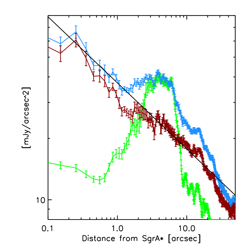
Figure 5: Left: Mean diffuse SB profiles in the $K_{S}$ wide-field image before (blue) and after (red) subtraction of the appropriately scaled Pa $\alpha$ emission (green; multiplied by arbitrary factor to optimise the plot). The straight black line is the best power-law fit to the red data within $R\leq 25"$ pc (corresponding to $R\lesssim 1$ pc for a GC distance of 8 kpc).

Figure 5 shows the measured surface brightness (SB) profile for the wide-field $Ks$-image, for the Paschen $\alpha$ emission, and the wide-field SB profile after a scaled subtraction of the latter. The continuous black line is the best-fit power law to the data at $R\leq 1.0$ pc. It has a reduced $\chi^{2}=14.3$, $\Sigma_{0}=16.4\pm 0.1$ mJy arcsec^-2, and $\Gamma=0.32\pm 0.01$. The relatively high $\chi^{2}$ is mainly due to systematic deviations of the profile from a power-law at certain restricted ranges of $R$. We found that these deviations are mainly related to the difficulties of precise subtraction of bright stars at small $R$. These systematics are slightly different for each data set that we present in this work (see, e.g. Fig 6), but do not significantly affect the overall result. The formal uncertainties resulting from the fit code have been rescaled to a reduced $\chi^{2}=1$ here and for all other fits reported in this paper. In appendix B we study several potential sources of systematic errors, such as sky offset, binning, fitting range, or application of the extinction correction. The sky offset, a probable systematic effect from inaccurate sky background subtraction and diffuse foreground (i.e. nor originating within the GC), was estimated on small regions of dark clouds (see Fig. 4) and subtracted prior to measuring the SB on the wide field image.

3.2 Br $\gamma$

The surface brightness in the Br $\gamma$ narrow band filter image is an interesting test case because here the emission from the ionised gas will provide a relatively large fraction of the overall diffuse emission. The resulting raw and ionised-gas-corrected SB profiles are shown in panel (a) of Fig. 6. A simple power-law provides a very good fit, with the best-fit power-law exponent of $\Gamma_{in}=0.23\pm 0.01$.

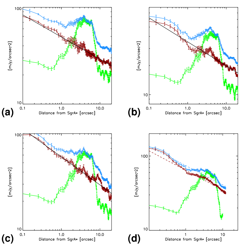
Figure 6: (a) Plot of the $Br\gamma$ diffuse SB profile before (blue) and after (red) subtraction of the appropriately scaled Pa $\alpha$ emission (green; multiplied by arbitrary factor to optimise the plot). The black line is for the best-fit power-law in the range $R\leq 25"$ pc (corresponding to $R\lesssim 1$ pc for a GC distance of 8 kpc). (b) As (a), but for the deep $K_{s}$ image. (c) As (a), but for the $H$ image. (d) As (a), but for the $K_{s}$ S13 image.

3.3 Deep $K_{S}$-band image

Here, we analyse the deep $K_{S}$ broad band image that we use for measuring the stellar number surface density in Paper I. The SB profiles are shown in panal (b) of Fig. 6. A simple power-law provides a very good fit, with the best-fit power-law exponent of $\Gamma_{in}=0.25\pm 0.01$.

3.4 $H$-band image

Analysing the diffuse flux in an $H$ band image represents, among others, a test in a regime, where differential extinction is stronger, where the sky background behaves in a different way, and where the ratio of line emission relative to Pa $\alpha$ is different. Also, due to increased anisoplanatic effects, point-source-subtraction removal is more difficult in $H$ than in $K_{s}$. Hence, the $H$-band can be very helpful in constraining systematic effects. We had to correct the $H$-band image for a systematic negative offset of the sky background, which could be measured on some small dark clouds in the field. The SB profiles are shown in panel (c) of Fig. 6. A simple power-law provides a good fit, with the best-fit power-law exponent of $\Gamma_{in}=0.29\pm 0.01$.

3.5 Deep $K_{S}$ image with S13 camera

As a final test, we examine the diffuse light density in a deep, multi-epoch $K_{S}$-band image obtained with data from the S13 camera of NACO/VLT. A simple power-law provides a good fit, with the best-fit power-law exponent of $\Gamma_{in}=0.26\pm 0.01$. We tested again the systematics of subtracting the stars down to different limiting magnitudes ($K_{s,lim}=16,18,20$). The power-law index changes between $0.25\pm 0.01$ and $0.29\pm 0.01$ and the plot looks similar in all cases (not shown). Compared to the NACO S27 $K_{s}$ data there appears to be an offset of the SB towards brighter values. We could not identify the source of this offset, but we note that it does not affect our main conclusions, in particular the existence of a power-law cusp and its index.

3.6 IB227 image

As a final test we used the IB227 image from Buchholz et al. (2009). A simple power-law provides a good fit, with the best-fit power-law exponent of $\Gamma_{in}=0.19\pm 0.01$. We do not show the corresponding fit in Fig. 6 to not overcrowd the plot. It is very similar to all the other plots.

4 Discussion

4.1 Mean projected power-law index

Table 1: Best-fit power law indices for the diffuse stellar light inside of $R<0.5$ pc. All formal uncertainties are $\leq 0.01$ after having been rescaled to a reduced $\chi^{2}=1$ , i.e. we are dominated by systematics.

Data	$\Gamma_{in}$
$K_{S}$, wide field	0.32
Br $\gamma$	0.23
$K_{S}$ deep field	0.25
$H$	0.29
$K_{S}$ S13	0.26
IB227	0.19

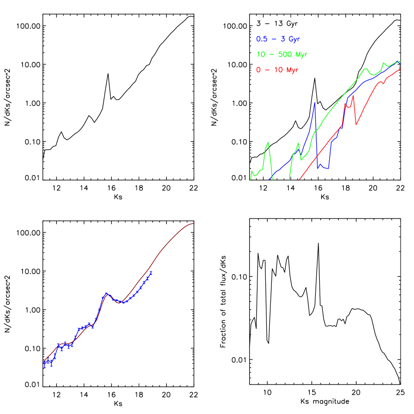
Figure 7: Estimates of the KLF within $R\leq 1$ pc of Sgr A*. Upper left: Model $K_{S}$ luminosity function (KLF) based on the star formation history derived by Pfuhl et al. (2011). Upper right: KLFs for stellar populations in certain time windows, using the star formation model by Pfuhl et al. (2011). Lower left: The red line is the model KLF smoothed with a Gaussian kernel to roughly take differential extinction into account. The blue line with error bars is the KLF as determined in Paper I. Lower right: Fraction of total flux contributed by stars of different magnitudes, i.e. the KLF multiplied by the flux density of stars in a given bin and divided by the total flux. Please note the different range of the x-axis in this plot, which is chosen to show the decrease of the flux contribution at $K_{s}>22$.

As the preceding sections have shown, measuring the diffuse stellar light around Sgr A* is a non-trivial undertaking and subject to potentially significant systematic effects. In particular, we have demonstrated that the mini-spiral contributes significantly to the measured diffuse flux at projected distances $R<0.5$ pc from Sgr A*, even when broad-band filters are used. If not taken into account, this will result in an apparent steep increase of the diffuse flux at $R\lesssim 0.4$ pc and then an almost flat SB profile in the innermost $\sim$$0.2$ pc. The exact systematic effect due to the mini-spiral will depend, of course, on the filter used. It is very strong in Br$\gamma$ and weaker in $K_{S}$ and $H$ (see Fig. 6).

The subtraction of the flux of both the bright stars and the gas and dust is prone to systematic errors. Fortunately, these errors will change with the observing conditions, for example seeing and adaptive optics correction, camera used, or observing wavelength. For this reason, we have used several completely independent data sets that were obtained at different times and with significantly different setups: Deep and shallow images, broad and narrow band observations, shorter and longer wavelength filters. It is satisfying to see that the resulting SB profile is consistent among all the data sets.

All our different measurements of the projected stellar surface brightness can be fit well by the simple model of a single power-law at $R\lesssim 1$ pc. The corresponding power-law indices are consistent with each other and also with the power-law index inferred for the stellar number density of faint stars in this region, as determined in Paper I. As studied and explained in detail in appendix B, the systematic error is dominated by effects of potential additive sky offsets and fitting range. The atmospheric contribution of the former is, however, variable in nature between sets of different observations and is therefore absorbed into the statistical error from the mean of the different values for $\Gamma$ observed. The latter is mainly caused by a systematic steepening of the slope with increasing $R$ and contributes an estimated $0.05$ to the uncertainty budget of $\Gamma$. As concerns the contribution of a potential source of diffuse emission from a stellar foreground population, for example in the nuclear disc, we do not take it into account here. We note, however, that its contribution would always be an additive offset. If taken into account, this would systematically steepen the observed $\Gamma$.

Table 1 lists the resulting best-fit power-law indices for the projected diffuse light in the inner $1.0$ pc. From these measurements to independent data sets we obtain a mean estimate of $\Gamma=0.26\pm 0.02_{stat}\pm 0.05_{sys}$. This value is smaller than, but agrees within its uncertainties, with what we observe for the number density of the stars in the range $17.5\lesssim K_{S}\lesssim 18.5$ that we present in Paper I. We conclude that the projected surface density distribution of stars around Sgr A* can be described well by a single power law with the same exponent for different stellar populations. The faint stars do not show a flat, core-like distribution as has been observed for the bright ($K_{S}\lesssim 15.5$) giants in the GC (Buchholz et al. 2009; Do et al. 2009; Bartko et al. 2010). The faint stellar population around Sgr A* clearly displays a power-law cusp in the central parsec. Given our measurements, assumptions, and analysis, we can exclude a flat projected core around Sgr A* with high confidence. Also, we do not find it necessary to use any broken power-law for the SB profile at projected radii $R\leq 1$ pc, as it was used by previous authors (e.g. Genzel et al. 2003; Schödel et al. 2007; Do et al. 2009).

4.2 What kind of stars contribute to the diffuse SB?

The stars that contribute dominantly to the diffuse light in our point-source subtracted images must be fainter than $K_{S}=18$. To obtain a better understanding of which kind of stars contribute dominantly to the diffuse SB, we study the $Ks$ luminosity function (KLF). First, we use the star formation history for the central parsec derived by Pfuhl et al. (2011) to construct a theoretical KLF. We used their Eq. (3) to compute the masses of nine single age stellar populations. The ages were taken to be the middle of the intervals $10-13$ Gyr, $8-10$ Gyr, $3-8$ Gyr, $1-3$ Gyr, $0.5-1$ Gyr, $200-500$ Myr, $50-200$ Myr, $10-50$ Myr, and $0-5$ Myr. We emphasise the illustrative nature of our model, which is not constructed to provide a precise fit to our data.

The model KLFs were calculated assuming Solar metallicities and Chabrier lognormal initial mass functions (see, http://stev.oapd.inaf.it/cgi-bin/cmd_2.8 and Chabrier 2001; Bressan et al. 2012; Chen et al. 2014, 2015; Tang et al. 2014).

The resulting total KLF and the individual contributions of the populations of different ages (where we summed over four broad age ranges) can be seen in the upper panels of Fig. 7. The lower left panel compares the smoothed (to take into account differential extinction and measurement uncertainties) model KLF to the completeness corrected KLF determined by us in Paper I. The agreement is satisfactory. The peaks around $K_{S}\approx 15.5$ arise from Red Clump (RC) stars. We point out that we have not made any specific effort to match the model KLF to the measured one, except for applying a scaling factor. Studies of star formation history or metallicity are beyond the scope of this paper.

The bottom right panel in Fig. 7 shows the fraction of the total flux contributed by the stars in the different bins of the model KLF. As can be seen, stars in the regime $K_{S}=19-22$ do not differ significantly in their overall weight. We expect these stars, to dominate our measurements of the diffuse light density. As can be seen in the upper right panel, these stars belong predominantly to the oldest stellar population. They will be of type G to F, have masses $\lesssim 1.5\,M_{\odot}$ and will live for several Gyrs (see also Fig. 16 in Schödel et al. 2007). They can thus be old enough to be dynamically relaxed and serve as tracers for the existence of a stellar cusp.

In Paper I we discuss and take into account the possible contamination of the surface number density of $K_{s}\approx 18$ stars by young stars from the most recent, $\sim$5 Myr-old star formation event in the central $R<0.5$ pc (see, e.g. Genzel et al. 2010; Lu et al. 2013). It turns out to be relatively minor, but the contamination from other young or intermediate-age populations, with ages $\lesssim 3$ Gyr may be significant. Here we want to explore whether such contamination could, in principle, also be present in the diffuse light. While we cannot completely rule out this possibility, the top right panel of Fig. 7 shows that stars older than a 3 Gyr will be a factor of a few more frequent than younger stars at $K_{s}>20$ (see also Fig. 11 in Paper I).

Also, although the stellar number density profiles derived in Paper I and the SB profile measured in this work probe different stellar masses and ages, the corresponding values of the power-law indices are approximately consistent with each another. Hence, while it is difficult to constrain quantitatively the contamination of our tracer populations by stars that are too young to be dynamically relaxed, this contamination must either be small or very similar across the different stellar magnitude ranges. The similarity of the power-law indices that we find for different tracers suggests that they may indeed be representative for the actual underlying structure of the old stars, which are expected to dominate the mass of the NSC.

As discussed in Paper I, the youngest stellar population is concentrated within $0.8\leq R\leq 12"$, or $0.03\leq R\leq 0.5$ pc, of Sgr A*. It cannot be dynamically relaxed and the corresponding stars are therefore inadequate tracers of the putative cusp. We cannot directly measure the contamination of our SB profiles by pre-main sequence stars, but we can estimate it. Since the surface density of young stars is strongly peaked towards Sgr A*, this contamination is more severe at small $R$. As Figure 12 in Paper I shows, the number density of pre-MS stars at $K_{s}\approx 20$ is roughly two orders of magnitude below the one from the other stars at $R=2"$. We therefore conclude that contamination by pre-MS stars is not an issue for the SB profiles presented here.

As can be seen in the upper right panel of Fig. 7, the population younger than 500 Myr could contaminate significantly star counts at magnitudes $17\lesssim K_{s}\lesssim 19$. The importance of this effect can currently not be well constrained because it depends on the unknown distribution of stars in this age range. On the other hand, the surface brightness measurements are dominated by older stars. The fact that we observe similar surface densities and brightnesses in Paper I is reassuring and suggests that contamination effects are not severe.

4.3 Optimised overall SB profile

Mainly for illustrative purposes, we produced a ’best’ corrected image by combining the corrected S13 and S27 wide-field images. The images were matched via a least-squares minimisation of an additive offset and a multiplicative scaling factor. We then measured the SB profile again as in section 3.1, that is we also estimated the uncertainty from inaccuracies in the sky background subtraction. This case is very similar to the $K_{s}$ wide field data and a simple 2D power-law provides a good fit to the data in the range $R\leq 1.0$ (blue dashed line in Fig. 8). The best-fit parameters are: $\Sigma_{0}=15.6\pm 0.1\,$mJy and $\Gamma=0.31\pm 0.01$. We note that the fit deviates systematically from the data at $R\gtrsim 25"$ (see also case of $K_{s}$ wide field data shown in Fig. 5). This may suggest the necessity to use of a broken power-law. However, this is not compelling once we take projection effects into account. A projected 3D simple power-law can fit the data well, as is shown by the straight orange line in Fig. 8 and discussed in more detail in the following section.

4.4 The 3D structure of the cluster

Our observations provide us with the surface brightness, but we would like to know the intrinsic structure of the NSC. This is not a trivial problem because it involves projection effects and requires a fairly complete and accurate knowledge of the stellar distribution on large scales both in and around the NSC. While we do not yet possess very detailed knowledge – in terms of high angular resolution and multi-wavelength observations – on the stellar population and its distribution at large scales, we can use the results of previous work on the large scale structure of the NSC combined with some basic or simplifying assumptions (such as spherical symmetry) to provide an approximate, general picture.

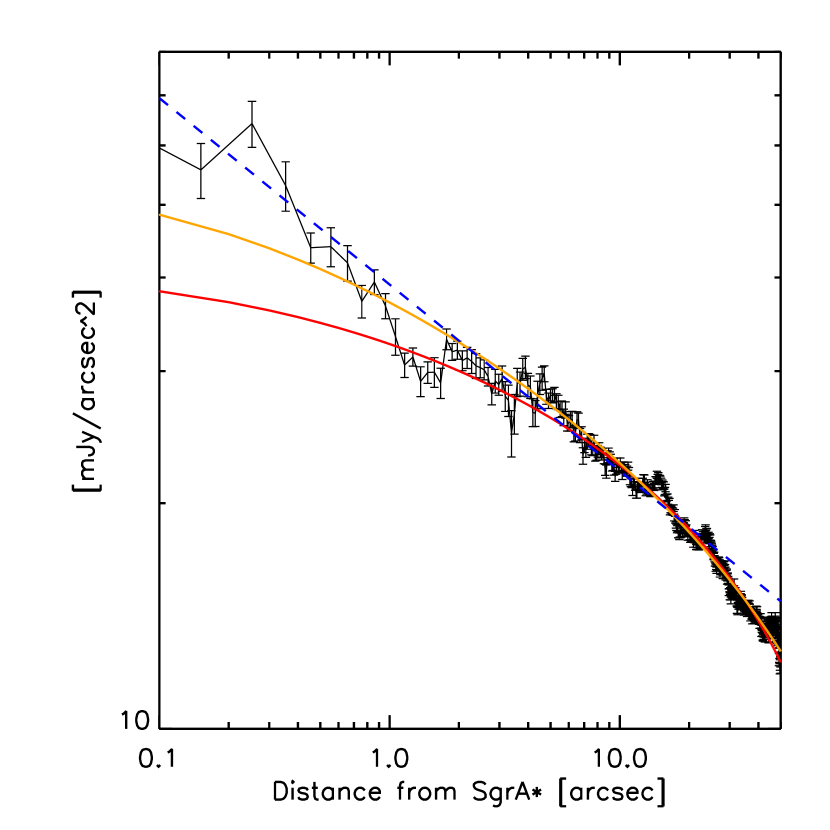
Figure 8: Black points: SB profile from the optimised $K_{s}$ wide plus $K_{s}$ S13 image, corrected for extinction and gas emission. The dashed blue line is a 2D simple power-law fit to the data at $R\leq 25"$ (1 pc). The straight lines are best fit projected 3D simple power-laws, assuming a simple model, where the stellar density drops to zero at outer cut-off radii of 10 pc (red) and 20 pc (orange).

As a first, purely illustrative approximation to the problem, we assume a simple - and inaccurate - model, in which the intrinsic 3D structure of the cluster is described by a simple power-law with an outer cut-off, where the stellar density drops abruptly to zero. We use the combined $K_{s}$ wide field plus $K_{s}$ S13 data (see section 4.3). They are shown in Fig. 8 along with a best fit 2D simple power-law model and two best-fit projected 3D simple power-law SB models for two different outer cut-off radii. We note several points: (1) For a cluster of finite extent, the projected SB is not given by a simple power-law. Instead, the SB continuously flattens towards small $R$. The larger the outer cut-off radius, the closer the projected SB profile resembles a simple power-law (as can be expected). (2) For small clusters (or small assumed outer cut-off radii)), the change in the projected power law within $R\approx 10"$ is so strong that a broken power-law may represent a better fit to the projected SB profile. In fact, such a broken power-law was frequently used in the past (e.g. Genzel et al. 2003; Schödel et al. 2007; Buchholz et al. 2009; Do et al. 2009). (3) In all cases, our simple toy model provides a surprisingly satisfactory fit to the data, with the best-fit value for the three-dimensional power-law index ranging between $\gamma=0.9-1.1$ (smaller value for the smaller cut-off radius).

Table 2: Best-fit model parameters for the Nuker fits to the SB profiles.

ID	$r_{b}$	$\gamma$	$\beta$	$\rho(r_{b})$
	(pc)			(mJy arcsec-3)
1a	$3.1\pm 0.1$	$1.11\pm 0.01$	$3.8\pm 0.1$	$0.029\pm 0.002$
2b	$2.9\pm 0.2$	$1.16\pm 0.01$	$2.9\pm 0.1$	$0.029\pm 0.003$
3c	$3.4\pm 0.2$	$1.17\pm 0.02$	$3.5\pm 0.2$	$0.023\pm 0.002$
4d	$3.0\pm 0.1$	$1.12\pm 0.01$	$3.6\pm 0.1$	$0.029\pm 0.001$
5e	$3.0\pm 0.1$	$1.12\pm 0.01$	$3.6\pm 0.1$	$0.029\pm 0.001$
6f	$3.1\pm 0.1$	$1.12\pm 0.01$	$3.7\pm 0.1$	$0.029\pm 0.002$
7g	$3.2\pm 0.2$	$1.15\pm 0.02$	$3.3\pm 0.1$	$0.027\pm 0.003$
8h	$3.2\pm 0.2$	$1.15\pm 0.02$	$3.5\pm 0.2$	$0.026\pm 0.003$
9i	$3.2\pm 0.2$	$1.15\pm 0.02$	$3.3\pm 0.1$	$0.027\pm 0.003$
10j	$3.2\pm 0.1$	$1.14\pm 0.01$	$3.9\pm 0.1$	$0.028\pm 0.002$
11k	$3.4\pm 0.2$	$1.20\pm 0.02$	$3.4\pm 0.2$	$0.027\pm 0.02$
12l	$3.1\pm 0.1$	$1.12\pm 0.01$	$3.7\pm 0.1$	$0.029\pm 0.002$
13m	$3.0\pm 0.1$	$1.13\pm 0.01$	$3.6\pm 0.1$	$0.033\pm 0.001$
14n	$3.3\pm 0.1$	$1.09\pm 0.01$	$3.8\pm 0.1$	$0.023\pm 0.001$
16o	$2.3\pm 0.1$	$1.05\pm 0.02$	$3.0\pm 0.0$	$0.046\pm 0.002$
17p	$3.4\pm 0.1$	$1.14\pm 0.01$	$4.0\pm 0.0$	$0.024\pm 0.001$
19q	$3.6\pm 0.2$	$1.15\pm 0.02$	$3.6\pm 0.2$	$0.019\pm 0.002$
20r	$3.0\pm 0.2$	$1.15\pm 0.02$	$3.1\pm 0.2$	$0.028\pm 0.003$

Assuming an intrinsic simple power-law structure is, of course, an oversimplification because a large body of previous studies of the stellar density in the GC indicates that the nuclear cluster follows a density of approximately $n(r)\propto r^{-2}$ outside of the central parsec, with a steepening slope at larger distances (see, e.g. references and discussions in Launhardt et al. 2002; Schödel et al. 2007, 2014a; Fritz et al. 2016). A steepening density profile is also required to avoid that the cluster mass diverges. Now we will explore the consequences of a steeper density slope at larger distances on the inferred three-dimensional power-law near Sgr A*.

To constrain the stellar distribution on scales of approximately 1 to 20 pc, we use the data on the flux density of the NSC from Schödel et al. (2014a) and Fritz et al. (2016). The former used extinction-corrected Spitzer $4.5\,\mu$m surface brightness maps. The latter used extinction corrected near-infrared data from NACO/VLT, WFC/HST, and VISTA. Both data sets are not adequate to sample the light density profile inside $R\approx 1\,$pc. The Spitzer data of Schödel et al. (2014a) are of low-angular resolution and long wavelength and completely dominated by a few bright stars and by emission from the mini-spiral in the inner parsec. The data from Fritz et al. (2016) are, in principle, more suitable, but are dominated by RC stars and brighter giants. As is well known and as we confirm in Paper I, these stars show a core-like structure within $R\leq 0.3$ pc from Sgr,A*.

A caveat is that this previous work was focussed on significantly brighter stars than what we are examining in the present work. The data by Schödel et al. (2014a) and Fritz et al. (2016) trace easily detectable stars and not the diffuse light density from very faint stars as analysed in this paper. Nevertheless, for simplicity – and because we assume that it is a good approximation on large scales – we will assume that the distribution of all populations is described well by these data. A study of the density of different stellar populations throughout the nuclear cluster out to distances beyond a few parsecs is beyond the scope of this work and will be addressed in a later paper. Again, we note that both in Paper I and in this work we find similar profiles for stellar components in significantly different brightness ranges, which supports our assumption that the individually detectable stars can be used as a good proxy for the cluster shape on large scales.

To isolate the nuclear cluster from the emission of the nuclear disc and Galactic Bulge, we used the Sérsic models for the non-NSC emission listed in Table 2 of Schödel et al. (2014a). They were scaled to the data at $R\geq 18$ pc and subtracted from the data sets from Schödel et al. (2014a) and Fritz et al. (2016), respectively. We then scaled the latter data to our data in the ranges $1.5\,\mathrm{pc}\leq R\leq 2.0\,$pc. At $R<1.5$ pc, we used exclusively our data. We then applied a 3D ’ Nuker’ model and projected it onto the sky to fit the measured surface brightness. We use the Nuker model (Lauer et al. 1995) in the form of Equ. 1 of Fritz et al. (2016):

$$\rho(r)=\rho(r_{b})2^{(\beta-\gamma)/\alpha}\left(\frac{r}{r_{b}}\right)^{-\gamma}\left[1+\left(\frac{r}{r_{b}}\right)^{\alpha}\right]^{(\gamma-\beta)/\alpha}.$$ (2)

Here, $r$ is the 3D distance from Sgr A*, $r_{b}$ is the break radius, $\rho$ is the 3D density, $\gamma$ is the exponent of the inner and $\beta$ the one of the outer power-law, and $\alpha$ defines the sharpness of the transition. We explicitly point out that the Nuker model was previously always used for 2D data, while we use it as a convenient mathematical model to describe the 3D shape of the cluster. The density was then projected along the line of sight via an integral:

$$\Sigma(R)=2\int_{r}^{\infty}\frac{r\rho(r)dr}{\sqrt{r^{2}-R^{2}}}.$$ (3)

For numerical reasons, to avoid a singularity, we could not integrate down to $r=R$ and therefore set the minimum $r=R+0.001$ pc. The best-fit was found with the IDL MPFIT package (Markwardt 2009). Uncertainties were re-scaled to a reduced $\chi^{2}=1$. We fixed the parameter $\alpha=10$ and used only data at $R\leq 20$ pc. Two of the fits, using the azimuthally averaged data of Schödel et al. (2014a) and Fritz et al. (2016) are shown in Fig. 9 (We note that the plots corresponding to all fits performed by us have a very similar appearance).

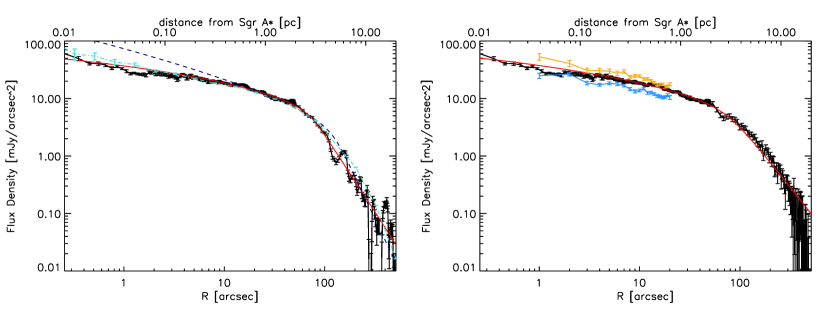
Figure 9: Nuker model fits (red solid lines) to the diffuse SB in the GC. Left: The data at $R\geq 1.5$ pc are the azimuthally averaged, extinction corrected Spitzer $4.5\,\mu$m data from Schödel et al. (2014a) minus model to remove the contribution from components not part of the NSC. The dashed blue line is a fit with a forced inner slope of $\gamma=1.5$, corresponding to the lighter stars in a two-component Bahcall-Wolf cusp (Bahcall & Wolf 1977). The dash-dotted turquoise line indicates the SB profile of the faint stars in the simulated cluster of Paper III. Right: The data at $R\geq 1.5$ pc are the azimuthally averaged, extinction corrected near-infrared data from Fritz et al. (2016) minus a model to remove the contribution from components not part of the NSC. The orange points and line show the stellar surface density data from Paper I for stars in the interval $K_{S}=17.5-18.5$ and blue for $K_{S}=16.5-17.5$. For better visualisation, the stellar surface densities have been scaled by constant, arbitrary factors.

There are a number of obvious systematic uncertainties related to this procedure. Our primary test of robustness is, of course, the use of the completely independent data sets of Schödel et al. (2014a) and Fritz et al. (2016). We then explored the parameter space by repeating the fitting procedure for different cases:

• Fit with the azimuthally averaged data of Schödel et al. (2014a) as well as their profiles along the Galactic Plane and perpendicular to it, to examine the influence of the flattening of the nuclear cluster.

• Flux offset due to non-NSC emission: We used different models from Schödel et al. (2014a) to estimate the fore- and background emission.

• Fits with different settings for the minimum integration boundary ($r=0.001$ and $0.01$ pc).

• Fits for fixed different values of $\alpha=5,30$.

• Fits to the entire data and fits limited to $R<10$ pc to examine the influence of the fitting region.

• Fits with a fixed parameter $\beta=3.0,4.0$.

Table 2 contains the best-fit parameters that we obtained for the model-fits to different data and under different assumptions and constraints. The $\chi^{2}$ values and the uncertainties of the different models and parameters are similar to each other. We can obtain an approximate, mean model for the nuclear cluster by taking the mean of each best-fit parameter and its standard deviation (not error of the mean; we do not include fixed parameters in these means): $r_{b}=3.1\pm 0.3$ pc, $\gamma=1.13\pm 0.03$, $\beta=3.5\pm 0.3$, and $\rho(r_{b})=0.028\pm 0.005$ mJy arcsec^-3. It is important to note that there are covariances between these parameters. For example, the value of $\rho(r_{b})$ depends clearly on the value of $\beta$, with larger $\beta$ related to smaller $\rho(r_{b})$. Co-variance is also present between $r_{b}$ and $\beta$. On the other hand, the mean values are fairly well constrained and provide us with a good approximation of the overall 3D shape of the NSC. Finally, and most importantly with respect to the aim of this paper, the value of $\gamma$ is relatively tightly constrained and does not vary much between the different fits.

Theory predicts that the cusp follows a power-law inside the break radius and that the latter is on the order of the radius of influence of the black hole, which has been found to be $\sim$$3-4$ pc (e.g. Alexander 2005; Feldmeier et al. 2014; Fritz et al. 2016; Feldmeier-Krause et al. 2017), consistent with The Nuker law break radius determined here and in Paper I.

Here, we are most interested in the question of the existence of a stellar cusp. As we can see, the three-dimensional power-law index $\gamma$ can be determined robustly and is insensitive to the potential systematics that we have considered. Due to the finite structure of the cluster $\gamma$ is not exactly equal to $\Gamma+1$. The latter would only be valid for a simple power-law cluster with infinite extent. We assume that the systematic uncertainty of $\Gamma$, estimated to amount to $0.05$ in section 4.1, applies also to $\gamma$. So, our best estimate for the 3D power-law index of the Milky Way’s NSC in the innermost 1-2 parsecs is $\gamma=1.13\pm 0.03_{model}\pm 0.05_{sys}$, where the first uncertainty term is estimated from our Nuker model fits with different assumptions and constraints as listed in Table 2 and the second term is due to the measurements on different independent data sets as derived in section 4.1. Based on the value of $\gamma$ and its uncertainty, we can rule out a flat core with high confidence.

An extensive analysis of the stellar number and flux surface density in the GC was presented in Fritz et al. (2016). They fitted a so-called $\gamma$-model and found that the radial structure of the NSC in the innermost few $0.1$ pc can be well described by a power-law with index $\gamma=0.90\pm 0.11$ for the stellar surface density and $\gamma=0.76\pm 0.08$. for the flux density. These values are flatter than what we have found here for the inner slope of the cluster. The main difference between their work and our work is that we focus on the diffuse emission of the faintest stellar population while their measurements are dominated by giant stars.

In Paper I we show that the stars of $K_{S}\approx 17$ and $K_{S}\approx 18$ show a projected surface density that is consistent with the one that we find here for the diffuse light, while the giants show a flattening inside a projected radius of $R\approx 0.3$ pc. In Fig. 9 we overplot the stellar surface number densities onto the plot of the surface brightness density of the diffuse light.

We find, however, larger values of $\gamma$ in Paper I. For the $K_{s}\approx 18$ stars we find $\gamma=1.41\pm 0.06\pm 0.1_{sys}$. This discrepancy may indicate certain biases related to the different methods. For example, we may have underestimated the dynamically unrelaxed stars may contaminate the star counts, as discussed in Paper I or we may over-estimated incompleteness due to crowding. Alternatively, we may have over-corrected the emission from gas and dust in this work, there may be a bias from the sky background subtraction resulting from an observational setup that was not optimised for measuring the unresolved, diffuse emission, or the different values reflect uncertainties in the scaled matching of our measurements and literature data at $R>1.5$ pc. There may also be other systematic effects at play that we have not considered. We note, however, that both values for $\gamma$ exclude a flat, core-like profile with high confidence. Their difference can provide us with a robust estimate of the true systematic uncertainty of both values, which may thus be on the order of $\Delta\gamma_{sys}=0.15$.

In Paper III (Baumgardt et al. arXiv:1701.03818) we compare the measurements to N-body simulations and confirm the consistency between measurements and theory. The probably best explanation for the flatness of the observed cusp is mass segregation between stars of different masses in the inner parts of the nuclear cluster, which flattens the density profile of bright stars away from the $\gamma=1.75$ prediction of Bahcall & Wolf (1976). In addition, due to repeated star formation and/or cluster infall not all the stars in the nuclear cluster may be old enough to be fully dynamically relaxed, which could cause a further modification of the central slope. Most models created so far assumed clusters with a single age stellar population that evolved for many relaxation times. The NSC of the Milky Way, on the other hand, contains stellar population of different ages (see, e.g. Pfuhl et al. 2011). Also, the NSC may have had less than a Hubble time for two body relaxation processes to work, so it may not be fully relaxed. Paper III presents more elaborate theoretical models, based on direct N-body simulations and explicit consideration of the star formation history of the NSC (modelled according to the one derived in Pfuhl et al. 2011), that provide results consistent with our data. We believe that the relative flatness of the cusp is the reason why it has eluded any clear confirmation for decades.

As concerns the value of $\beta$, which describes the density decrease at distances $r>>r_{b}$, we find in Paper I a value $\beta_{resolved}=3.4\pm 0.3$, which agrees well with the value derived here and in earlier work on the large-scale structure of the NSC (see introduction and references in Schödel et al. 2007). As a final note, the data used here to constrain the cluster structure at large $R$ reflect a much brighter tracer population than the stars that dominate the diffuse emission from unresolved stars in our NACO images.

4.5 Density of stars near Sgr A*, enclosed stellar mass

For observational purposes, it is of great interest to obtain a rough estimate of the surface number density of unresolved stars at $R=0.25"$ ($R=0.01$ pc). On the one hand, the results from Paper I show that the surface number density of stars at $17.5\leq K_{s}\leq 18.5$ is about 20 arcsec^-2 at $R=0.25"$. Applying this normalisation to the model KLF from section 4.2, this corresponds to 80 stars arcsec^-2 in the interval $18.5\leq K_{s}\leq 19.5$ and 370 stars arcsec^-2 in the interval $19.5\leq K_{s}\leq 20.5$. If we use the surface flux density derived in this work, on the other hand, we obtain somewhat different, but consistent, values. The extinction-corrected surface flux density estimated at $R=0.01$ pc is about 50 mJy arcsec^-2, which results, for the same model KLF, densities of 64 stars arcsec^-2 in the interval $18.5\leq K_{s}\leq 19.5$ and 300 stars arcsec^-2 in the interval $19.5\leq K_{s}\leq 20.5$. The comparison between the numbers of faint stars obtained by these two estimates points to an uncertainty of about $20\%$. An additional source of uncertainty, also on the order of $20\%$, results from the exact normalisation of the KLF. Here we assumed that the diffuse flux is dominated by stars $19\leq K_{s}\leq 22$. NIR cameras at the next generation of extremely large telescopes, such as MICADO/E-ELT (Davies & Genzel 2010), will have angular resolutions of $\lesssim 10$ mas FWHM, and thus be able to resolve surface number densities on the order of 1000 stars arcsec^-2 (the actual performance will depend on the dynamical range and luminosity function of the observed field). Hence, the future generation of ground-based, AO-assisted telescopes will be able to observe the stellar cusp around Sgr A* directly, down to about one solar mass stars. The high stellar surface density is encouraging for interferometric observations of the immediate environment of Sgr A* with an instrument such as GRAVITY/VLTI (Eisenhauer et al. 2011), if it can reach the required high sensitivity.

Table 3: Stellar mass densities near Sgr A* and total stellar mass within $r=1\,pc$.

ID	$\rho(1\,\mathrm{pc})$	$\rho(0.1\,\mathrm{pc})$	$\rho(0.01\,\mathrm{pc})$	$m_{stellar}(1\,\mathrm{pc})$
	(M⊙ pc-3)	(M⊙ pc-3)	(M⊙ pc-3)	M⊙
1a	$1.5\times 10^{5}$	$2.0\times 10^{6}$	$2.7\times 10^{7}$	$1.0\times 10^{6}$
2b	$1.8\times 10^{5}$	$2.4\times 10^{6}$	$3.2\times 10^{7}$	$1.2\times 10^{6}$
3c	$1.6\times 10^{5}$	$2.2\times 10^{6}$	$3.0\times 10^{7}$	$1.1\times 10^{6}$
4d	$1.2\times 10^{5}$	$1.6\times 10^{6}$	$2.2\times 10^{7}$	$0.8\times 10^{6}$

Another value of interest is the mass density near Sgr A* and the total enclosed mass within 1 pc of Sgr A*. Using our best-fit Nuker-law parameters, we have computed the mass density at distances of $r=1,0.1$, and $0.01$ pc from Sgr A*, using five different normalisations of the enclosed mass, four of them dynamical (Schödel et al. 2009; Feldmeier et al. 2014; Chatzopoulos et al. 2015; Fritz et al. 2016) and one of them based on mass-to-light ratio (Schödel et al. 2014a). The values are listed in Table 3 and agree within factors of less than two.

Densities in excess of a few $10^{7}$ M_⊙ pc^-3 are reached at $r<0.01$ pc of Sgr A*, which corresponds roughly to the apo-centre of the orbit of the short-period star S2/S0-2 (e.g. Boehle et al. 2016). This is comparable to what has been inferred by some models for the central density of Omega Centauri (Noyola et al. 2008). We note that $0.01$ pc correspond to about $0.25"$ or a few resolution elements of a 10m-class telescope in the NIR at the distance of the GC. In spite of this high density, the small volume implies that this corresponds to only $180\pm 30$ M_⊙ (taking the mean and standard deviation of the estimates resulting from the different normalisations).

From the different values given in Table 3, we estimate a total stellar mass within $r=0.1$ pc of Sgr A* of about $1.3\pm 0.1\times 10^{4}\,$M_⊙, smaller than, but of the same order of magnitude as, the value given by Yusef-Zadeh et al. (2012). The total mass within $r=1$ pc of Sgr A* is $1.0\pm 0.1\times 10^{6}\,$M_⊙ and within $r=3$ pc of Sgr A* is $7.8\pm 0.6\times 10^{6}\,$M_⊙, roughly twice the mass of Sgr A*. As a note of caution, we remind the reader here that the Nuker model assumed here for the NSC does not take into account the mass from the nuclear bulge or other stellar components that do not form part of the NSC, but may overlap with it. Therefore, our model will under-estimate the real mass enclosed at large $r$.

We point out that here we assume a constant mass-to-light ratio throughout the NSC. This may result in an under-estimation of the enclosed mass of the NSC at small radii. Theoretical considerations and simulations predict an accumulation of stellar-mass black holes in an invisible, steep ($\gamma\approx-1.75$) cusp around Sgr A* (e.g. Morris 1993; Merritt 2006; Alexander & Hopman 2009; Preto & Amaro-Seoane 2010). This cusp is actually steeper when one considers realistic number fractions for the stellar population, which leads to a more efficient segregation of the masses. In particular, Alexander & Hopman (2009), Preto & Amaro-Seoane (2010), and Amaro-Seoane & Preto (2011) find in their models that the cusp for their ’heavy’ stars, the precursors of stellar-mass black holes, build up a cusp with $\gamma\approx-2$. They refer to this finding as “strong mass segregation”. Depending on the properties of this putative black hole cusp, the enclosed mass at small distances from Sgr A* may be significantly higher than the estimates provided here. The most recent constraint on the extended mass within $0.01$ pc of Sgr A* from the orbital analysis of individual stars is that it must be less than $1.3\times 10^{5}$ M_⊙ (Boehle et al. 2016). Hence, the mass density estimated here can be easily accommodated by current dynamical analyses.

5 Conclusions

This paper presents the radial surface brightness profile of the diffuse emission in high angular resolution, point source-subtracted images of the GC. After taking into account the contamination of the diffuse light by line emission from gas and dust in the mini-spiral, we argue that the diffuse emission arises from a faint, unresolved stellar population with magnitudes of $K_{S}=19-22$. This corresponds to main sequence stars or sub-giant stars with masses of about $0.8-1.5\,M_{\odot}$. These stars can live long enough on the main sequence to be dynamically relaxed and thus to serve as a tracer population for a stellar cusp around the central black hole of the Milky Way.

We find that the projected surface brightness profile can be fitted well by a power-law slope with an index of $\Gamma_{in}=0.26\pm 0.02_{stat}\pm 0.05_{sys}$ at $R<0.5$ pc. This value is smaller than, but consistent with what we find for the stellar surface number density of $K_{s}\approx 17$ and $K_{s}\approx 18$ (observed magnitude) stars in Paper I. An important caveat is that we cannot directly determine which kind of stars we are observing and the contamination of the star counts by young, dynamically unrelaxed stars may be high, as discussed in Paper I. However, the fact that the work in this paper and in Paper I use different methodologies, but arrive a similar results, gives us confidence in our results.

Translating these results into an intrinsic, three-dimensional description of the cluster is not trivial, but by using previous studies of the cluster morphology on large scales as constraints, along with a spherical approximation, we find that the cluster can be described well by a three-dimensional Nuker law within about 20 pc of the central black hole. According to our models, the break radius is $3.1\pm 0.3$ pc contains about a stellar mass of twice the mass of Sgr A* and thus coincides with the radius of influence of the black hole (e.g. Alexander 2005). The three-dimensional density inside of the break radius follows a power law with an exponent $\gamma_{in}=1.13\pm 0.03_{model}\pm 0.05_{sys}$. A core-like distribution of the faint stars can thus be firmly excluded. From a comparison between the results for the faint, unresolved stellar population and the faint resolved population (Paper I), we suggest that a robust range for the power-law index of the cusp is $\gamma=1.1-1.4$.

An underlying assumption of our work is that the faint emission arises indeed mostly from stars old enough to be dynamically relaxed. A possible source of concern could be contamination by pre-main sequence stars in the region of the few million year-old starburst within $R=0.5$ pc of Sgr A*. Our analysis, in Paper I, of the KLF of the stars in the inner parsec, shows that this possibility is rather unlikely.

The stellar cusp identified in this work and in Paper I is flatter than the one predicted for single-mass stars around a massive central black hole $\gamma_{theor}=1.75$, or for low-mass stars in a cluster composed of two mass groups ($\gamma_{theor}=1.5$). In contrast to the simplifying assumptions of previous theoretical work, the nuclear cluster at the GC has undergone multiple epochs of star formation and/or cluster infall. Thus, not all the stars may be old enough to be fully dynamically relaxed. As we will elaborate in Paper III, our observations nicely agree with the detailed, direct-summation Nbody simulations.In Paper III we compare the measurements to N-body simulations and confirm the consistency between measurements and theory.

The flatness of the cusp is one of the main reasons why it may have eluded detection so far. The second reason is that the giant stars brighter than $K_{S}\approx 16$ dominated all previous attempts at determining the NSC’s structure. However, these stars show a core-like profile in projection within $R\approx 0.3$ pc (see Paper I and discussion and references therein).

We summarise our conclusions here:

1. Our study of the diffuse stellar light around Sgr A* confirms the existence of a simple power-law cusp around Sgr A*, with a 3D power-law index $\gamma\approx 1.13\pm 0.03_{model}\pm 0.05_{sys}$.

2. The cusp is shallower than what is predicted by theory.

3. The existence of a cusp in our Galaxy supports the existence of stellar cusps in other, similar systems that are composed of a nuclear cluster and a massive black hole.

4. The existence of stellar cusps is an important prerequisite for the observation of EMRIs with gravitational wave detectors.

5. The bright giants and the Red Clump stars at the GC do not show the same distribution as the fainter stars. Either the bright giants are, on average, younger than the fainter stars and are not yet dynamically sufficiently well relaxed, or some mechanism has altered the appearance of this population: Possibly, the envelope of giants were removed by colliding with the fragmenting gas disc at the GC which later turned into the observed stellar disc of young, massive stars (Amaro-Seoane & Chen 2014).

Future research needs to be done to refine our understanding of the cusp at the GC. On the observational side, we need to infer robust data on the large-scale two-dimensional distribution of stars out to about 10  pc from Sgr A* with high sensitivity and angular resolution. We will then be able to reconstruct the intrinsic three-dimensional profile of the cluster. The next step will then be an accurate determination of the different types of faint stars near Sgr A* (e.g.: Which ones are pre-MS stars?) in order to understand the age structure of the nuclear star cluster. At least some of this future work can only be done with a 30m-class telescope. Observations with the next generation of telescopes can test the predictions on stellar number densities from our work.

Appendix A Photometric accuracy and recovery of diffuse light with StarFinder

In this section we explore two issues via simulations of the Galactic Centre: (1) Photometric accuracy and point-source residuals when the PSF varies across the field due to anisoplanatic effects. (2) The capability of recovering the diffuse light with Starfinder in a GC-like environment and with a spatially variable PSF. As a test case we use observations of NACO through the Br$\gamma$ filter, where the diffuse background is particularly high and variable due to the strong line emission from the minispiral.

The simulated images are based on the Br$\gamma$ observations described in section 2. We used stellar sources detected down to $K_{s}=18$, where the star counts are reasonably complete across the field and source detection is highly reliable. The guide star PSF was extracted from IRS 7 in the original Br$\gamma$ data, after having repaired the saturated core of IRS 7. To simulate the variation of the PSF across the field, we modelled the loss of Strehl and elongation of the PSFs via convolution with Gaussian kernels. The latter are chosen as being elongated along the line connecting any given star to the guide star, a typical manifestation of anisoplanatic effects. The FWHM of the Gaussians along these lines grows by $0.027^{\prime\prime}$ for every $10^{\prime\prime}$ distance from IRS 7 and by $0.008"$ in the perpendicular direction. In this way we obtain a simulated image that appears similar to the original image, albeit with a somewhat stronger anisoplanatic effect, which is good because it means that we are carrying out our simulations for a conservative test case. We use a FWHM of the PSF of about $0.08"$ for the guide star. At a distance of $20"$ from the guide star, the PSF has a FWHM of about $0.1"$ along the line connecting it with the guide star.

Finally, we added readout and photon noise (both from sources and from the sky). We then carried out runs of StarFinder both with a constant and with a variable PSF, the latter as described in section 2.

We simulated images with a flat, zero background, with a complex background by including the minispiral, and with a complex background that includes the minispiral and an additional diffuse power-law component. As described in section 2, we do not fit the background with StarFinder, that is, the keywords $BACK\_BOX$ and $ESTIMATE\_BG$ are set to zero. Instead, we determined the diffuse light directly from the point-source-subtracted images. As a side note, we point out that throughout this paper we use the terms background and diffuse emission in an equivalent way.

In all simulated images, we first repaired the core of the PSF of the brightest star, IRS 7. Although it was not saturated in the simulated images, of course, it is saturated in the real data and this step is necessary because if forms an integral part of the data reduction. It will lead to a slight broadening of the guide star’s PSF because its core is replaced by the median of the cores of nearby stars, that have a somewhat lower Strehl. We note that we wrote our own code for repairing the core of IRS 7 because the native StarFinder code for this purpose, REPAIR_SATURATED.PRO will only work accurately if the complete PSF is known a priori. However, this is not the case here, where we actually use the brightest, saturated star to estimate the broad, extended wings of the PSF. We mention this problem here because it may arise in most similar situations where a user wants to repair the cores of saturated stars with StarFinder. The key is that, while StarFinder only applies a multiplicative scaling factor, one must also use an additive offset when fitting the core to the saturated star.

When we apply PSF fitting with a variable PSF, we sub-divide the simulated image into overlapping square fields of $10.8"$ size on a side, that we call ’sub-images’. A local PSF is estimated from the brightest, isolated stars in each field. Subsequently, the wings from the bright guide star are fitted to this local PSF and PSF fitting is performed on each sub-image. The sub-images overlap by half of their size. When recomposing the point-source-subtracted images, the borders of the sub-images (about $2"$ width) are removed and the remaining overlapping areas are averaged. In this way we can create a homogeneous residual image.

A.1 Variable PSF and constant zero background

Our first test is performed with a constant background of value zero. Several images and plots that evaluate this test quantitatively are shown in Fig. 10.

We can see that the residuals are significant and systematic in case of using only a single, constant PSF. They are significantly smaller and more constant across the field when we use a variable PSF. Quantitatively, this effect can be seen nicely in the plot of the differences between measured and input magnitudes for the stars. They show a systematic trend with distance from the guide star in case of use of a single PSF. With a variable PSF, some local systematics appear (as expected because we do not model the PSF for each position), but they are far smaller. In general, systematic photometric uncertainties due to PSF variability are on the order of just a few $0.01$ mag when we use a variable PSF. As concerns the measured background, after point-source subtraction, it is close to zero, but has a small, positive bias that increases with distance from the guide star. This trend can possibly be partially explained by the fact that measurements become less accurate towards the image edges because we cannot minimise uncertainties by multiple measurements in overlapping fields near the edges and because the potential PSF reference sources are fewer and fainter towards the image edges. Variable PSF fitting performs better in background recovery than constant PSF fitting. We also note that there is a small dip of the recovered background close to the position of Sgr A*. We believe that this is due to the strong concentration of bright stars there. It appears that the broadening of the PSF caused by the necessary superposition of several reference stars leads to negative residuals close to bright stars. In any case, the positive residual is very small. It is, in the worst case, not more than a few percent of the surface brightness of the mini-spiral or diffuse stellar emission that we analyse in this work. We thus conclude that it is safe to ignore it. We also conclude that using a variable PSF is superior to using a constant PSF and that a constant flat background $\gtrsim 1.0$ mJy arcsec^-2 can be accurately recovered by our method.

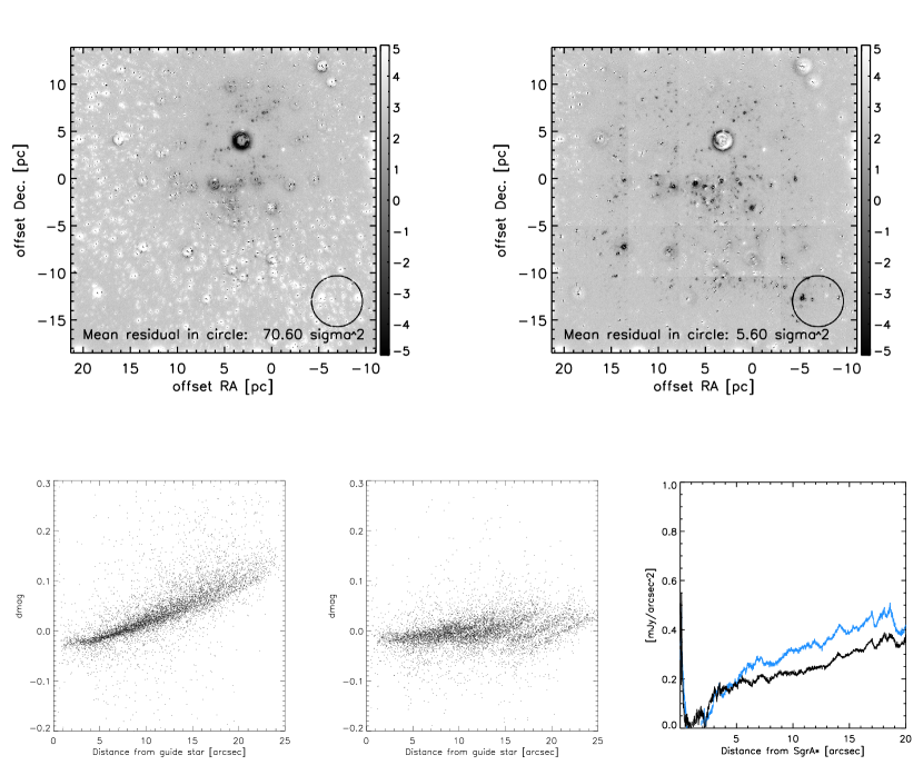
Figure 10: PSF fitting test with a variable PSF and a constant background. Upper left: Point-source subtracted image after use of a single, constant PSF. The circle in the lower right shows a region in which we measured the sum of the squared residual, which is $70.6\,\sigma^{2}$ for this region. Upper right: Like upper left, but after using a variable PSF. The sum of the squared residual in the circle is $5.6\,\sigma^{2}$. The grey scales are expressed in terms of $\sigma$ deviations from the noise image. Bottom left: Differences between the measured magnitudes of stars and their input magnitudes when a single, constant PSF is used. Bottom centre: Differences between the measured magnitudes of stars and their input magnitudes when a variable PSF is used. Bottom right: Plot of background, after point-source subtraction, as a function of distance from Sgr A*. The background is the median in rings around Sgr A*. The blue data are for the case of a single PSF and the black data for the case of a variable PSF.

A.2 Variable PSF plus complex diffuse emission from gas

To model highly complex diffuse emission we used the HST Paschen $\alpha$ image of the minispiral, transformed it to the frame of the NACO Brackett-$\gamma$ image, and scaled its flux accordingly. Some smoothing was applied to mitigate the effects of interpolation. Then we proceeded as described above. In Fig. 11 we show the simulated image after fitting and subtracting the point-sources and the residual after, additionally, subtracting the input gas emission. Finally, we show the plot of residual light density as a function of distance from Sgr A*. It is close to zero at all distances, very similar as in the case of a flat, zero background. We conclude that our variable PSF fitting with StarFinder can reproduce very well the details of complex diffuse emission and that the residual light can be reproduced accurately after the complex diffuse emission is removed. Here, we remind the reader again that we do not fit the diffuse emission with StarFinder. We just fit and subtract the point-sources.

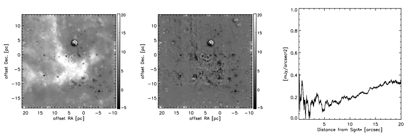
Figure 11: PSF fitting test with a variable PSF and a complex, diffuse background. Left: Point-source subtracted image after use of a variable PSF. Middle: Residual image, after subtracting the input distribution of diffuse emission. Right: Background as function of distance from Sgr A* as measured in the residual image. The grey scales are expressed in terms of $\sigma$ deviations from the noise image.

A.3 Variable PSF plus gas and power-law cusp

Finally, we added a power-law cusp from faint, diffuse stellar emission to the simulated image, proceeding as described in the previous sections. The cusp was simulated as a pure power-law with a 2D exponent of $\Gamma=-0.2$, a scale radius of $R_{0}=12.5"$, and a flux density of 10 mJy arcsec² at $R_{0}$. In Fig. 12 we show the simulated image after fitting and subtracting the point-sources and the residual after, additionally, subtracting the gas emission. Finally, we show the plot of residual light density as a function of distance from Sgr A* with the input cusp model over-plotted. The recovered power-law cusp is almost identical to the input model, with minor deviations only near the edge of the field and near Sgr A*.

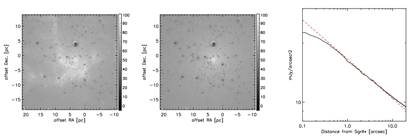
Figure 12: PSF fitting test with a variable PSF, complex, extended emission from gas/dust, and diffuse emission from a population of unresolved faint stars. Left: Point-source subtracted image after use of a variable PSF. The grey scale is expressed in terms of $\sigma$ deviations from the noise image. Middle: Residual image, after subtracting the input distribution of diffuse emission. Right: Background as function of distance from Sgr A* as measured in the residual image. The dashed red line is the power-law cusp used as input. The grey scales are expressed in terms of $\sigma$ deviations from the noise image. We note that the scales are different from the ones used in in Fig. 11

A.4 Variable PSF: Real data

Finally, we will take a closer look at the performance of our methodology with real data. For this purpose we use the $H-$band image used in this work. The point-source-subtracted images for a constant PSF (panel a)) and use of a variable PSF (panel b)) are shown in Fig. 13. Significant systematic residuals related to point-sources can be seen in case of the constant PSF. Moreover, those residuals vary strongly with position in the field. We point also out that the real data show a different residual pattern than the simulated data. In particular, the residuals look less symmetric than in case of the simulated data. We believe that this can probably be explained by time-variable AO performance because the final mosaic image is the result of observations of four different pointings. Variable AO perfomance is a frequent feature of AO instruments and is mostly related to changes in the atmospheric seeing. We did, however, not further investigate this effect here because it would go far beyond the purpose of this paper.

The point-source-subtracted image after using a variable PSF shows smaller residuals that are more homogeneous across the field. The total squared residuals are significantly lower than in case of a constant PSF. We note that the residuals here do still include diffuse emission from gas and unresolved stars.

Panel c) of Fig. 13 shows the full extent of the PSF halo. It can be seen that it extends out to almost $2^{\prime\prime}$ from the the centre of the PSF. Panels c) and d) show zooms onto the cores of locally estimated PSFs. It can be seen that the PSF core near the image edge, at roughly $15"$ from the guide star, is elongated compared to the PSF core near the image centre.

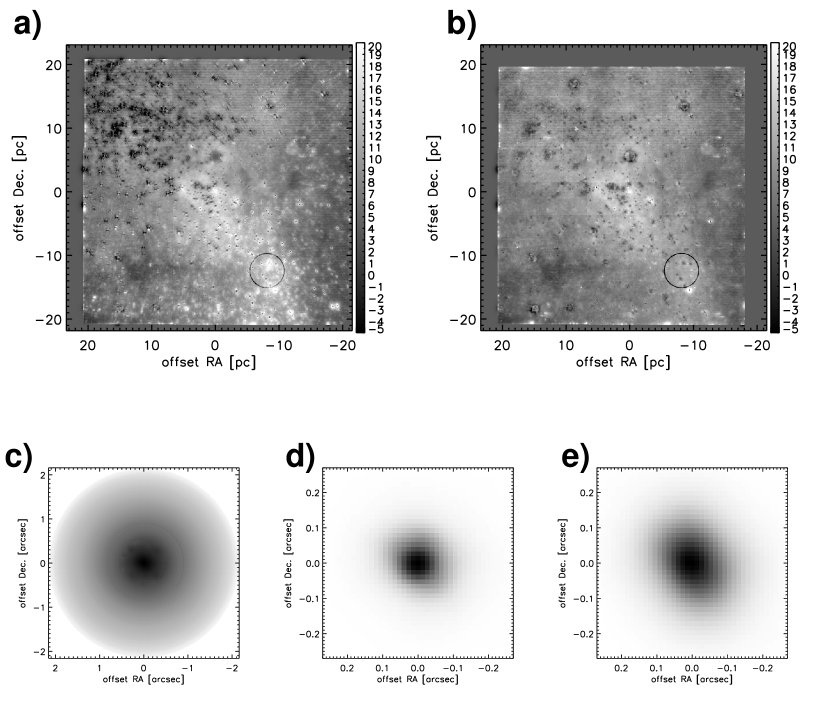
Figure 13: PSF fitting test with a variable PSF on the H-band image used in this work. a) Point-source-subtracted image after use of a single, constant PSF. The circle in the lower right shows a region in which we measured the sum of the squared residual, which is $131\,\sigma^{2}$. b) Point-source-subtracted image after use of a variable PSF. The circle in the lower right shows a region in which we measured the sum of the squared residual, which is $41\,\sigma^{2}$. c) Full extent of the PSF. d) Zoom onto core of PSF near image centre. e) Zoom onto core of PSF near the lower right corner. All grey scale are logarithmic.

The conclusion of this appendix is that our variable PSF fitting with StarFinder with subsequent point-source-subtraction is well suited to recover the complex diffuse emission from gas/dust and, after removal of the latter, to measure the diffuse distribution from a faint, unresolved stellar population at the GC.

Appendix B Systematic errors of the 2D fit of the SB profile

In this section we examine several potential sources of systematic errors in the power law plus scaled gas emission fits to the SFP profiles of the $K_{s}$ wide field image. The results are readily applicable to the images in other filters.

B.1 Sky subtraction

Our experiments with the data suggest that the strongest systematic effect can arise from an unknown additive offset of the diffuse emission. Although the images were sky-subtracted – the sky background in the corresponding filters was measured on a dark cloud at a few arcminutes offset – there is some uncertainty related to this procedure: There was only one sky measurement done for the approximately one hour-long observations. Hence, the sky background may have varied. Also, we are interested in the SB profile of the nuclear star cluster, but there may be diffuse flux contributions from other structures, such as the nuclear stellar disc (see Launhardt et al. 2002). Fortunately, there are several dark clouds contained in the field-of-view (FOV). Those clouds belong most probably to dense gas and dust in the so-called circumnuclear ring (CNR) in front of the nuclear star cluster (see, e.g. Ekers et al. 1983; Lo & Claussen 1983; Christopher et al. 2005) and can thus serve to estimate the flux offset. We measured the median flux density at six positions within these dark clouds (see blue circles in Fig. 4) and thus obtained an estimate for the mean and standard deviation of the constant diffuse flux offset in the $K_{s}$ wide field image: $0.3\pm 0.1$ mJy arcsec^-2 (corresponding to roughly $5$ mJy arcsec^-2 if corrected for 3 mag of extinction). The surface flux density measurement was then repeated after subtracting this mean offset. The extinction correction was performed after the subtraction of this potential background bias. The resulting SB profile and best fit model is shown in panel a) of Fig. 13, with the best-fit parameters listed in row 3 of Tab. 4. It can be seen that uncertainty about an additive offset from the sky or from diffuse foreground radiation can have a significant (order $20\%$) effect on the measured value of $\Gamma$ – and, by consequence, also on $\beta$.

Since in this work we analyse observations with different filters and instrument setups and taken under different conditions, we expect that we can accurately estimate the contribution from the variability of the atmospheric emission from the standard deviation of the results for the different filters (at least for $\Gamma$). As concerns the possible contribution of a diffuse component from Galactic structures in the foreground of the NSC, in particular the nuclear disc, its effect will always be a positive offset. That means that, if we subtract such an offset, $\Gamma$ would increase.

B.2 Extinction correction

The strong differential extinction in the central parsecs of the Milky Way is well known and we correct for it in our measurements. If we assume simply a constant extinction and do not correct for its variation, then the reduced $\chi^{2}$ becomes higher and the gas-subtracted SFP profile can be fit less well with a power-law. The normalisation of the SB changes by $<10\%$ and $\Gamma$ becomes steeper (see panel b) in Fig. 14 and row 2 in Tab. 4). The latter is to be expected because extinction is lower near Sgr A* (see, e.g. extinction maps presented in Schödel et al. 2007, 2010).

In any case, this is an extreme test that overestimates the uncertainties probably significantly because, after all, interstellar extinction and its variation towards the GC have been investigated well and can be robustly estimated (e.g. Schödel et al. 2007; Buchholz et al. 2009; Schödel et al. 2010; Nishiyama & Schödel 2013; Hosek et al. 2015; Fritz et al. 2016). We therefore repeated our analysis twice, once with the extinction map smoothed by a Gaussian of $2"$ FWHM and once with the extinction map smoothed by a median filter in a box of of $4"$ width. In these cases the final results agree, within the uncertainties, with our best estimate. We conclude that the correction for variable interstellar extinction is not a significant source of systematic error in this work.

B.3 Completeness effects

When studying stellar number densities, as in Paper I, assessing and correcting incompleteness due to sensitivity and, in particular, crowding can have significant effects on the results. In our study of the diffuse light density, bias related to completeness could occur as well. The contribution of the occasional bright star on the mean surface brightness at a given $R$ will be negligible due to our use of the ROBUST_MEAN procedure, that rejects outliers and produces values very similar to the median. However, in small, crowded areas, such as the central arcseconds near Sgr A*, subtraction of faint stars may be significantly less complete so that, on average brighter stars remain in the image than in less crowded areas, which may create a systematic effect.

To examine this effect, we studied the SFP profile in images, in which stars down to different magnitude levels were subtracted: $K_{s}=16$, $K_{s}=18$, and all detectable stars. The $3\,\sigma$ detection limit for stars in the $K_{S}$ wide field image is about $K_{S}\approx 19$ (albeit at low completeness). The resulting profiles and best fits are shown in panel c) of Fig. 14. The corresponding best-fit parameters are listed in rows 5 and 6 of Tab. 4. Apart from an overall $\sim$$10-20\%$ shift between the measured SBs, the profiles look very similar. The best fit parameters - apart from the SB normalisation, $\Sigma_{0}$, - show only a small range of bias. In particular, no significant change of the best-fit parameters occurs whether we subtract all detectable stars or only stars down to $K_{s}=18$. We conclude that completeness effects are not any significant source of systematic error in this work.

B.4 Masking

As shown in Fig. 4, we mask several regions, that is, we exclude them from the analysis. These regions are extended dark clouds, residuals near the brightest star (IRS 7), objects with strong excess from line-emission or hot dust (e.g. IRS 1W, IRS 21, or IRS 13), or negative residuals around the densely clustered bright stars near Sgr A*. As panel d) in Fig. 14 and row 4 in Tab. 4 show, suppression of masking makes the fit noisier, but does not alter the best-fit parameters significantly. We conclude that the choice of masking applied in this work is not any significant source of systematic error.

B.5 Binning

We examined two different ways of binning the data. First, we binned the data in a way that each bin contained the same number of pixels. This will mean that the bins become smaller at larger $R$. A small ($\sim$15$\%$) increase of $\Gamma$ is observed (see panel e) in Fig. 14 and row 7 in Tab. 4). However, we have chosen an extreme case of binning ($1\times 10^{4}$ pixels or about 100 arcsec² per bin), which eliminates all data pints at $R<0.1$ pc. For a less extreme binning of 10 arcsec² per bin, the differences in the best-fit parameters are much smaller, with $\Gamma=0.25$.

We also tested logarithmic binning, which results in increasingly larger bins for larger $R$. As shown in panel f) in Fig. 14 and row 8 in Tab. 4, this produces no significant deviation in the best-fit parameters.

We conclude that binning is probably not any significant source of systematic errors in this analysis, but may contribute an uncertainty on the order of $\sim$$5\%$ to the value of $\Gamma$.

Table 4: Best-fit parameters for $Ks$ wide-field image, under different circumstances that may affect systematics. We note that all the formal uncertainties of the best-fit parameters are $\leq 1\%$, with the exception of row 8, which has significantly larger formal uncertainties due to the large reduced $\chi^{2}$. The $\chi^{2}$ listed here are smaller than the ones listed in Tab. 1 because the fitting range is different here ($R\leq 0.5$ pc compared to $R\leq 1$ pc in the main body of the paper; see discussion on the change of the projected power-law in sections B.6 and 4.4). Therefore they are not listed in this table, which serves to explore systematic uncertainties, which dominate the error budget.

	$\Sigma_{0}$	$\Gamma$	$\Sigma_{0}$	$\chi^{2}_{red}$
	(mJy arcsec-2)
1	$14.3$	$0.32$	$0.057$	$0.3$
2	$22.6$	$0.33$	$0.045$	$1.0$
3	$15.7$	$0.31$	$0.057$	$0.5$
4	$20.5$	$0.24$	$0.062$	$0.3$
5	$26.8$	$0.25$	$0.058$	$0.1$
6	$21.7$	$0.23$	$0.057$	$0.4$
7	$20.7$	$0.27$	$0.062$	$0.5$
8	$21.4$	$0.28$	$0.054$	$2.5$

• Final product as used in the results of this paper: Masking and extinction correction applied.

• No correction of differential extinction, assumption of $A_{Ks}=3.0$ constant.

• Masking and extinction applied. Subtraction of potential sky offset of $0.3$ mJy arcsec^-2.

• No masking applied.

• Stars only subtracted if they are brighter than $K_{s}=16$.

• Stars only subtracted if they are brighter than $K_{s}=18$.

• Like 1, but using bins with constant number of pixels ($1\times 10^{4}$) per bin.

• Like 1, but using bins of equal logarithmic width.

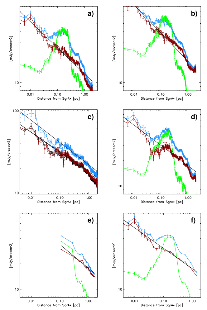
Figure 14: Fits of the SB profile from the $K_{s}$ wide field image to test potential sources of systematic errors. a) Subtraction of a potential sky offset. b) Assumption of constant extinction across the field. c) Subtraction of point sources down to $K_{s}=16$ (blue), $K_{s}=18$ (red), and all detectable point sources (back). d) No masking of dark clouds, or of systematic positive or negative residuals. e) Binning with a constant number of pixels ($1\times 10^{4}$) per bin. f) Logarithmic binning, leading to a higher weight of the inner bins.

B.6 Fitting range

Finally, we study the role of the range in $R$ used to fit the power-law from the stellar diffuse emission. When we only include data at $R\leq 0.4,0.6,0.8,1.0,1.2,1.5$ pc, we obtain $\Gamma=0.22,0.21,0.23,0.24,0.27,0.31$, and $\Sigma_{0}=21.3,21.7,21.3,20.9,20.4,20.3$ mJy arcsec^-2. As we can see, there is a systematic effect with the power-law becoming steeper at larger $R$. If we fit only data at $R\geq 0.5$ pc, then we obtain $\Gamma=0.40$ and $\Sigma_{0}=22.2$ mJy arcsec^-2. We show the corresponding fit in Fig. 15. On the other hand, if we fix the outer edge of the fitting range to $R=1.0$ pc and then use only data at $R\geq 0.2,0.4,0.6$ pc, we obtain $\Gamma=0.30,0.33,0.35$, and $\Sigma_{0}=21.5,21.7,22.0$ mJy arcsec^-2.

We conclude that the data from the $K_{s}$ wide field image show evidence for a steepening of the power-law with increasing $R$. When we analyse the SB profiles for the different observations in this work, we will always fit the power-law in the range 0 pc$\leq R\leq$1 pc. From our analysis here we estimate that the corresponding best-fit values of $\Gamma$ may have an associated systematic uncertainty on the order of $0.05$. The fitting range has only a minor contribution to the uncertainty of $\Sigma_{0}$, on the order of $3\%$.

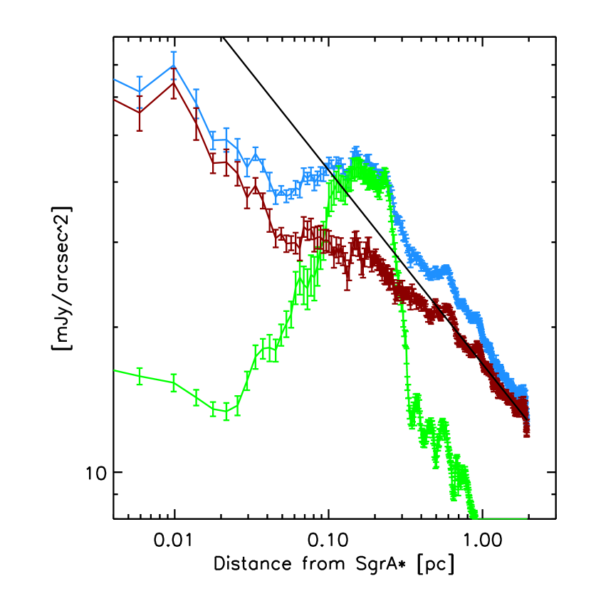
Figure 15: Mean diffuse SB profiles in the $K_{S}$ wide-field image before (blue) and after (red) subtraction of the scaled Pa $\alpha$ emission (green). the straight black line is a simple power-law fit to the data at $R\geq 0.5$ pc.

B.7 Conclusion on systematic uncertainties

From the study of the different potential sources of systematic errors in this section we identify three effects with possibly significant contribution: 1) An unknown additive sky offset, 2) the fitting range, and 3) binning. Effect 1) will, however, be absorbed by our using of several independent data sets. It will mainly be important in the sense of any contribution of a non-nuclear stellar population to the diffuse light and then always act to increase the estimated $\Gamma$. Effect 2) may contribute with a systematic error of $0.05$, compared to at most $0.02$ from 3), and will therefore dominate the budget of systematic errors. We will adopt $0.05$ as our systematic uncertainty for $\Gamma$.

As concerns the normalisation of the diffuse flux density, $\Sigma_{0}$ we cannot compensate potential atmospheric effects through the use of different filters. We therefore consider that a $25\%$ systematic uncertainty may be a good estimate of the systematic uncertainty for this parameter (see above). The effects of binning and of fitting range can be neglected for this parameter.