Self-Consistent Black Hole Accretion Spectral Models and the Forgotten Role of Coronal Comptonization of Reflection Emission

Abstract

Continuum and reflection spectral models have each been widely employed in measuring the spins of accreting black holes. However, the two approaches have not been implemented together in a photon-conserving, self-consistent framework. We develop such a framework using the black-hole X-ray binary GX  339–4 as a touchstone source, and we demonstrate three important ramifications: (1) Compton scattering of reflection emission in the corona is routinely ignored, but is an essential consideration given that reflection is linked to the regimes with strongest Comptonization. Properly accounting for this causes the inferred reflection fraction to increase substantially, especially for the hard state. Another important impact of the Comptonization of reflection emission by the corona is the downscattered tail. Downscattering has the potential to mimic the relativistically-broadened red wing of the Fe line associated with a spinning black hole. (2) Recent evidence for a reflection component with a harder spectral index than the power-law continuum is naturally explained as Compton-scattered reflection emission. (3) Photon conservation provides an important constraint on the hard state’s accretion rate. For bright hard states, we show that disk truncation to large scales $R>>R_{\rm ISCO}$ is unlikely as this would require accretion rates far in excess of the observed $\dot{M}$ of the brightest soft states. Our principal conclusion is that when modeling relativistically-broadened reflection, spectral models should allow for coronal Compton scattering of the reflection features, and when possible, take advantage of the additional constraining power from linking to the thermal disk component.

1. Introduction

Nature’s black holes are delineated by mass into two primary classes: supermassive ($M\gtrsim 10^{5}M_{\odot}$) and stellar mass ($M\lesssim 100M_{\odot}$), with any falling in-between termed intermediate mass. For a black hole of any mass, the no-hair theorem holds that the black hole is uniquely and completely characterized by its mass and its spin angular momentum. One of the principal challenges in modern astrophysics is to measure and understand the distribution of black hole spins ($a_{*}$).

One of the most widely-employed approaches for measuring black hole spin is through modeling fluoresced features in the reflection spectrum. The most prominent and recognized such feature is the Fe-K$\alpha$ line complex (Fabian et al., 1989; Brenneman & Reynolds, 2006; Brenneman, 2013; Reynolds, 2014). The term “reflection” here refers to the reprocessing of hard X-ray emission illuminating the disk from above. The illuminating agent is understood to be a hot corona enshrouding the inner disk, and the hard X-ray emission is attributed to Compton up-scattering of the thermal seed photons originating in the disk component (e.g., White & Holt 1982; Gierliński et al. 1999). The Compton emission from the corona has a power-law spectrum, which (generally) cuts off at high energies. A portion of this coronal emission returns to the disk and irradiates its outer atmosphere. The disk’s heated outer layer is photoionized, resulting in fluorescent line emission as the atoms de-excite. In addition to its forest of line features, the reflection continuum produces a broad “Compton hump” peaked at $\sim 30$ keV, above the Fe edge.

Relativity sets Doppler splitting and boosting as well as gravitational redshift for the reflection features produced across the disk. Each such feature is accordingly imprinted with information about the spacetime at its point of origin in the disk. A feature of principal interest is the Fe K line whose red wing is used to estimate the disk’s inner radius, which in turn provides a constraint on the black hole’s spin.

The other primary method for measuring black hole spin is via thermal continuum-fitting (Zhang et al., 1997; McClintock et al., 2014). In this case, the blackbody-like emission from the accretion disk is the component of interest, and spin manifests through the efficiency with which the disk radiates away the rest-mass energy of accreting gas. In effect, the spin is estimated using the combined constraint provided by the disk’s observed flux and peak temperature. For this method to deliver an estimate of spin, it is necessary to have knowledge of the black hole’s mass, the line-of-sight inclination of the spin axis, and the system’s distance.

The reflection method is applied to both stellar-mass and supermassive black holes, whereas continuum fitting is predominantly useful for stellar-mass black holes. Both methods rely upon a single crucial foundational assumption: that the inner edge of the accretion disk is exactly matched to the radius of the innermost-stable circular orbit (ISCO), which is a monotonic function of both mass and spin.

Although there is overlap in the set of BH systems which have measurements from each approach, the methods are optimized for opposing conditions; when a system is most amenable for one method, the other is generally hampered. For instance, for the thermal state in which continuum-fitting is most adept (e.g., McClintock et al. 2014; Steiner et al. 2009a), Comptonization and reflection are faint compared to the bright disk. Conversely, hard states are dominated by the Compton power law and its associated reflection (e.g., Fabian & Ross 2010), and here the thermal disk is quite cool and faint, often so weak that the thermal emission is undetected. As a result, both methods are not usually applied fruitfully to a single data set (see, e.g., Steiner et al. 2012). Instead, for transient black-hole X-ray binaries, one can apply both methods to observations at distinct epochs capturing a range of hard and soft states as the source evolves.

As consequence of this phenomenological decoupling between thermal and nonthermal dominance, the spectral models describing thermal disk emission versus Compton and reflection emission have largely undergone independent development. And as a result the cross-coupling between spectral components has been sparsely studied. One notable effort by Petrucci et al. (2001) explored the effect of coronal Comptonization on the reflection continuum flux and Compton hump, but in general this has gone unexplored. A handful of similar efforts have taken steps towards self-consistent treatment of the thermal and nonthermal spectral components – notably using eqpair (Coppi 1999; e.g., Kubota & Done 2016) or compps (Poutanen & Svensson, 1996), and to lesser degree Parker et al. (2016); Basak & Zdziarski (2016); Plant et al. (2015); Tomsick et al. (2014); Steiner et al. (2011); Miller et al. (2009). But an advanced self-consistent approach has not been realized. In this work, we examine several important aspects of a self-consistent model, sighted towards measuring black hole spin.

Adopting the usual assumption that the hard power-law photons originate in a hot corona that Compton scatters thermal disk photons, then by extension the reflection photons emerging from the inner disk will likewise undergo the same coronal Compton scattering. Recognizing this, as a first step towards self-consistency, we begin by examining the impact of coronal Comptonization on the reflection spectrum. This is particularly important for the hard state, in which Compton scattering is most pronounced. After touching upon this point, we go on to tackle the larger objective of producing an interlinked disk-coronal spectral model which imposes self-consistency. To connect with observations, we apply our model to the peak bright hard-state spectrum of GX 339–4, which is described in detail in García et al. (2015).

These data are among the highest-signal reflection spectra ever studied. Specifically, the data in question correspond to “Box A” in García et al. (2015, hereafter,G15), which is comprised of $>40$-million X-ray counts as collected by RXTE’s Proportional Counter Array (PCA; Jahoda et al. 2006) with a spectral range $\sim 3-45$ keV.

In G15, a simple spectral model was adopted, consisting of a cutoff power-law continuum, a component of relativistically broadened reflection (relxill), and a narrow component of distant reflection (xillver; i.e., located far from the regime of strong gravity and also far from the corona). In addition, a cosmetic Gaussian absorption feature was included in the model near the Fe complex at $\sim 7.4$ keV. For further details on the data and modeling procedure adopted, we refer the reader to G15.

G15 followed the common practices standard in reflection modeling of hard-state data, which do not include the self-consistent effects we introduce here. In G15, the reflection fits were found to clearly demand that reflection originate from a very small inner radius, a radius of $\lesssim 2\leavevmode\nobreak\ R_{g}$. And yet no thermal emission was required by the fit, although two reflection components were demanded (the broad and narrow components mentioned above). Given the high luminosity of this hard state, can the reflection fit be reconciled with the apparent dearth of thermal disk emission? What is the effect of including Compton-scattering on the reflection emission? Can a single reflection component, partially transmitted and partially scattered by the corona, account for the complete signal? Our work addresses these questions using the GX 339–4 data as a touchstone data for examining the impact of a self-consistent framework on black-hole spectral data as a general practice.

Section 2 describes our overall approach. We first focus on the impact of Compton-scattering on Fe lines in reflection spectra in Section 3, and then discuss a fully self-consistent approach in Section 4. In Section 5, we apply this prescription to GX 339–4. Finally, a broader discussion and our conclusions are given in Sections 6 and 7.

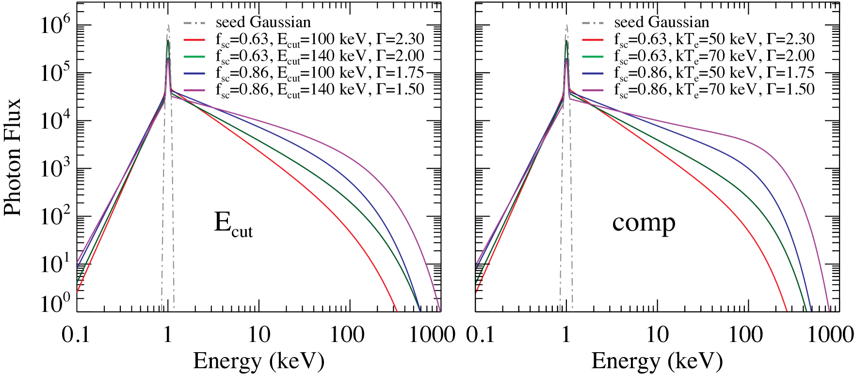
Figure 1.— The shape of the Compton-scattered continuum that results from seed photons input at 1 keV, for a range of coronal properties. We show the output of simplcut acting on an input Gaussian line at 1 keV using each of its two kernels: $E_{\rm cut}$ (left) which we adopt throughout the text, and comp (right) which is based on nthcomp and described in Appendix A. The values of $f_{\rm SC}$ correspond to $\tau=1$ and $\tau=2$ for uniform coronae with unity covering fraction. Note that here most line photons go into the scattered wings; these appear faint with respect to the peak because they are very broad even though they contain most of the signal. Of principal importance is the significant downscattered contribution from the line, which is appreciable and is steeper when $\Gamma$ is large.

Figure 2.— An illustration showing how downscattered reflection could plausibly mimic broad plus narrow reflection components and could therefore potentially be a source of systematic error in estimating spin. Top panels depict composite spectra modeled as either broad and narrow reflection or as a Comptonized narrow reflection component. The bottom panels present the profile of the modeled coronal scattering as acting on a narrow Fe line to illustrate its shape. For reference, we also overlay the shape of a relativistically broadened line with spin $a_{*}=0.9$. Note from the bottom panels that the broad relativistic line profile matches closely that of the Compton-downscattered wing for the hard state (with a steeper $\Gamma=1.5$), but for the soft state ($\Gamma=2.5$) the red wing is narrower.

Figure 3.— The effect of Compton scattering on a broad reflection component (relxill) component. The intrinsic emission (i.e., the reflection component for a completely transparent corona) is shown as a green solid line. The solid black line shows the net effect of Compton-scattering on this emission. Dashed and dotted black lines show the portions which have respectively scattered or been transmitted through the corona. The spectrum illustrated here was generated for $f_{\rm SC}=0.3$, $\Gamma=2$, and $E_{\rm cut}=100$ keV for the corona; $a_{*}=0$, $q=3$, $i=45\arcdeg$, log $\xi$=2, and a solar abundance of Fe for the disk. The bolometric photon count is identical for both curves; the apparent enhancement for the black curve in the 1–100 keV range is due to the $\nu F_{\nu}$ scaling, and is compensated at the lowest energies ($\lesssim 1\leavevmode\nobreak\ \rm keV$) at which the green curve is brighter (and which dominates the photon count).

2. Structuring a Self-Consistent Model

We focus on a self-consistent disk-coronal spectral model, in which the thermal disk emission, reflection, and coronal power-law are interconnected in a single framework. Our approach makes several simplifying assumptions. We firstly assume that the power-law component is generated by Comptonization in a thermal corona with no bulk motion, and that the corona is uniform in the sense that its temperature, optical depth, and covering factor are invariant across the inner disk (i.e., we ignore any radial gradients that may affect the corona-disk interplay). While we do not impose a particular geometry on the corona, we make the simplifying assumption that the corona emits isotropically. For a chosen geometry, an anisotropy correction (see e.g., Haardt & Maraschi 1993) could be applied to the reflection fraction; an investigation of such geometry-specific corrections is left for future work.

We assume that the disk is optically thick and geometrically thin and that it terminates at an inner radius $R_{\rm in}\geq R_{\rm ISCO}$. The boundary condition at the inner radius assumes zero torque. Spectral hardening (also commonly termed the “color correction”) describes the relationship between color temperature $T_{c}$ and effective temperature $T_{\rm eff}$, and it is defined as $T_{c}=fT_{\rm eff}$. The correction term $f$ is assumed to scale as $f\sim T_{c}^{1/3}$ (Davis & Hubeny, 2006). Radiation emitted by the disk that is bent back and strikes the disk due to gravitational lensing (i.e., “returning radiation”) is not considered here.

A fully self-consistent model of the accreting system should include the following couplings between components:

• disk-corona: A fraction $f_{\rm sc}$ of thermal accretion disk photons are Compton-scattered by the corona into the power-law component. Reflection photons, which originate at the disk surface, will also scatter in the hot corona. Photon conservation here ensures that the Compton power-law photons once originated as thermal disk emission.

• corona-reflection: The Compton-scattered photons which illuminate to the disk give rise to the reflection component. The reflection fraction describes the flux of Compton-scattered photons directed back to the disk relative to the Compton flux that is transmitted to infinity (Dauser et al., 2016). Properly incorporating photon counting ensures that the Compton-scattered disk photons are conserved and correctly apportioned between components. For instance, in this case photon conservation links the flux of the observed Compton power-law component to the flux of this same component from the vantage point of the disk (i.e., as prescribed by the reflection fraction).

• disk-reflection: The inner radius of the disk is tracked by two independent spectral characteristics: the red wing of the relativistic reflection features and the emitting area of the multicolor-blackbody disk. A self-consistent treatment of these two components is achieved by ensuring that the radius of the thermal emission in the soft state and the reflection component in the hard state mutually constrain the area of the thermal emission for the hard-state disk. At the same time, photon conservation provides a constraint on the temperature via the disk photon luminosity.

• corona/disk-jet: Although self-consistent modeling of the radio jet can constrain the hard-state geometry (see e.g., Coriat et al. 2011), the radio jet is beyond our scope is not considered in this work.

3. Compton-Scattering of Reflection Photons

We begin our investigation of self-consistent modeling with an in-depth examination of the coupling of the thermal disk photons and the coronal electrons which give rise to the Compton power law. The Compton scattering of thermal disk photons into a power-law component has been widely studied (e.g., Poutanen & Svensson 1996; Titarchuk 1994; Dovčiak et al. 2004; Zdziarski et al. 1996, and references therein). However, the impact of Compton scattering on the non-thermal reflection features emitted from the disk’s surface is typically ignored, though see Wilkins & Gallo (2015) and Petrucci et al. (2001).

As a first-order treatment, we can convolve the reflection spectrum with the Compton-scattering kernel such as simpl (Steiner et al., 2009b). This model redistributes a scattered fraction $f_{\rm SC}$ of seed photons into a post-scattering distribution via a Green’s function. The most basic implementation consists of a one- or two-sided power law distribution (Steiner et al., 2009a). In this paper we adopt the two-sided version and go one step further, introducing a more sophisticated implementation of simpl termed simplcut, which we will use throughout and which we now describe.

3.1. simplcut

simplcut is an extension of the simpl model that adopts a cut-off power-law shape for the Compton component. It is governed by four physical parameters: the scattered fraction $f_{\rm SC}$, the spectral index $\Gamma$, the high-energy turnover, and the reflection fraction ($R_{\rm F}$). We note that $f_{\rm SC}$ is distinct from the optical depth $\tau$; $f_{\rm SC}$, and $\Gamma$ are fitted, independent of $\tau$. This operationally allows for a variable (non-unity) covering factor of the corona above the disk. ($\tau$ can be inferred for a desired geometry using the spectral index and high-energy turnover terms.) $R_{\rm F}$ is defined as the number of scattered photons which return to illuminate the disk (i.e., those producing reflection) divided by the number which reach infinity. No prescription for angle-dependence is applied, which is equivalent to using the observed power-law flux as proxy for all flux at infinity.

Within simplcut are two options for the scattering kernel. The first kernel, which we adopt throughout unless otherwise specified, is shaped by an exponential cutoff $E_{\rm cut}$ and described by the following Green’s function, normalized at each seed energy $E_{0}$:

$$G(E;E_{0})dE\propto\begin{cases}(E/E_{0})^{-\Gamma}\leavevmode\nobreak\ {\rm exp}(-E/E_{\rm cut})dE/E_{0},&E\geq E_{0}\\ (E/E_{0})^{\Gamma+1}dE/E_{0},&E<E_{0},\end{cases}$$ (1)

The second kernel is based upon nthcomp (Zdziarski et al., 1996), with electron temperature $kT_{e}$ taking the place of $E_{\rm cut}$. This kernel and its implementation are described in Appendix A, and its shape is illustrated in the right panel of Figure 1. We opt to use the $E_{\rm cut}$ kernel throughout for the sake of its straightforward comparison with published results (though see Appendix A to see our modeling results using both kernels).

Figure 1 demonstrates simplcut’s effect, illustrating the net impact of the corona on a narrow 1 keV line viewed through coronae with a range of settings. The gray lines depict seed 1 keV photons. For a covering factor of unity, the familiar optical depth $\tau$ is related to the scattered fraction by $f_{\rm SC}=1-{\rm exp}(-\tau)$; electron temperature $kT_{e}$ and high-energy cutoff $E_{\rm cut}$ are approximately matched to one another using an approximate correspondence $E_{\rm cut}=2-3\leavevmode\nobreak\ kT_{e}$ (here we have arbitrarily selected $E_{\rm cut}=2\leavevmode\nobreak\ kT_{e}$ for presenting the kernels).

The most important feature to note is the prominent downscattering of the line by the hot corona (e.g., Matt et al. 1997), which is essentially identical between the two kernels. This is worth particular attention given that the red wing of reflection features are widely employed in estimating the inner-disk radius (and thereby the spin) of accreting black holes. Note also that the transmitted portion of the line remains narrow. In considering the Compton-scattering of reflection features, our prescription using simplcut greatly improves upon the present status quo, which is seen in the figure as the narrow gray line.

3.2. On Compton Downscattered Line Features

Given that Compton scattering produces emission that can contribute to the red wing of a line profile (notably the Fe line), this may plausibly impact spin measurements. We now explore this phenomenon in greater detail. The principal question before us is whether or not Compton downscattering can mimic the effect of strong gravity on fluorescent line emission. This is an important consideration given that the hard states in which reflection is widely studied is associated with strong Compton scattering.

As described by Eqn. 1, the shape of the downscattered emission is purely a function of $\Gamma$ (specifically, the downscattering spectral index is $-\Gamma-1$; also, see Pozdnyakov et al. 1983). Meanwhile, the shape of the red wing of a relativistic line is given principally by the spin of the black hole, but it is also affected by the line emissivity $q$ and inclination $i$.

For reference, using canonical values $q=3$ and $i=60\arcdeg$ we find the following correspondence between the shape of a red wing for a relativistic line (at a given $a_{*}$) and the downscattered wing of a narrow line due to Comptonization: $a_{*}=1$ matches $\Gamma\approx 1.5$, $a_{*}=0.7$ matches $\Gamma\approx 2.5$, $a_{*}=0.4$ matches $\Gamma\approx 3.5$, and $a_{*}=0$ matches $\Gamma\gtrsim 4$. It therefore follows that if Compton-scattering were being conflated with relativistic distortion, this can be revealed though examination of data spanning a range of $\Gamma$, or equivalently, a range of spectral hardness.

Ideally, one would examine both hard and soft (or steep-power law; Remillard & McClintock 2006) states to maximize this difference. One expects that any bias introduced by this effect would lead a harder spectrum to fit to a higher value of spin (or, equivalently, a smaller inner radius). We note that the most recent NuSTAR reflection studies of Cyg X–1 find $a_{*}=0.93-0.96$ for the soft state and $a_{*}>0.97$ in the hard state (Walton et al., 2016; Parker et al., 2015). The direction of this mismatch in spin (corresponding a factor $\sim 25\%$ difference in $R_{\rm in}$) is consistent with the type of bias one would expect from unmodeled coronal Comptonization.

We compare relativistic and Compton-scattering effects in Figure 2 in order to illustrate how the two may be confused. In the top panels, we present illustrative (simulated) spectra in black comprised of both broad and narrow reflection components (analyses using two reflection components being ubiquitous for AGN, and commonplace for stellar BHs). The broad component originates in the regime of strong gravity while the narrow component is produced from further away, where relativistic distortions are negligible. In red we illustrate that closely-matching spectra can be produced by instead Compton-scattering a single narrow reflection component. The left panels depict a representative hard-state spectrum with spectral index $\Gamma=1.5$, and the right panels a soft spectrum with $\Gamma=2.5$. (We note that many narrow-line Seyfert 1s show spectra with $\Gamma$ in this range, which may indicate that they have also have low $f_{\rm SC}$.) In the bottom panels, we show as red dashed lines the shapes of the corresponding Compton-scattering profile for a narrow Fe line. For each, the resulting lineshape is comprised of sharp transmitted and broad scattered components. As a reference, a relativistically broadened Fe-line profile for a spin $a_{*}=0.9$ is overlaid as a blue dotted line. Note the close correspondence between the high-spin relativistic line and the Compton wing for the hard state in the left-bottom panel; note also that the Compton-scattered lineshape for the soft state is not as broad as a high-spin (relativistic) line. In both cases the upscattered power law from the Fe line contributes an excess blueward of the line-center, which is potentially detectable in a general case. But since here the upscattered line lies significantly below the Compton continuum in flux, the effect has minor impact in these examples.

In Figure 3 we show the net impact of coronal Comptonization on a full relativistic reflection spectrum (modeled via relxill). This illustrates the generic case in which relativistic reflection features from an accreting black hole in an X-ray binary or AGN undergo Compton-scattering through the corona. The comingling of these effects applies the vast majority of X-ray reflection data of black holes, and motivates its presentation here. In the figure, a green line shows the naked reflection emission from a nonrotating black hole ($a_{*}=0$), i.e., the reflection component emitted by the disk prior to any coronal Compton scattering. After passing through a corona with $f_{\rm SC}=0.3$ and $\Gamma=2$, the scattered spectrum is both hardened and also smeared out in energy, with net result shown as the solid black curve. Note for the black curve that the $\sim 30$ keV Compton hump and the red wing of the $\sim 6.7$ keV Fe line are broader, and that the reflection features appear muted relative to an enhanced (and harder) continuum.

4. Towards a Composite Model

4.1. Model Components

As the primary feature of our full spectral model, we ensure a self-consistent linking of the fluxes between disk, Compton, and reflection components. Incorporating the effects of Comptonization by the corona described above, we adopt two basic models which we will employ in fitting GX 339–4 spectral data:

Model 1:

tbabs(simplcut$\otimes$(ezdiskbb+relxill)+xillver),

and

Model 2:

tbabs(simplcut$\otimes$(ezdiskbb+relxill)).

Model 1 is a reformulation of the typical spectral model employed for many supermassive and stellar black-hole systems (mentioned in Section 3.2), which consists of both broad (relativistic) and narrow reflection. Here, the narrow reflection is assumed to be produced far from the black hole, for instance in an outer disk rim. This distant emission would not undergo appreciable Compton scattering by a central corona. Because of this, we fix xillver’s setting for reflection fraction to -1 (the negative sign merely indicates that the continuum power-law is omitted), and fit for its normalization. Accordingly, we note that wherever a fit values of $R_{\rm F}$ is shown, this refers specifically to the relativistic reflection component. Model 2 is identical to Model 1 except that we consider just a single relativistic reflection component. Both include a first-order treatment of reflection and Compton scattering (but not higher order exchanges).

Although omitted from the descriptions above, when we apply these models to GX 339–4 we also include a Gaussian absorption line at $\sim 7.4$ keV (this line may be an instrumental artifact rather than physical in origin, and is discussed in great detail in G15. tbabs (Wilms et al., 2000) describes photoelectric absorption as X-rays traverse the line-of-sight interstellar gas column with $N_{\rm H}=5\times 10^{21}\rm cm^{-2}$ (Fuerst et al., 2016), a quantity which we keep fixed throughout our analysis.

ezdiskbb is a spectral disk model for a geometrically thin multi-color accretion disk with zero torque at the inner-boundary (Zimmerman et al., 2005). Importantly, ezdiskbb has been variously shown to recover essentially constant radii from soft black-hole spectra (e.g., Gou et al. 2011; Chen et al. 2016; Peris et al. 2016), demonstrating its utility here.

relxill and xillver are leading models of spectral reflection (García & Kallman, 2010; García et al., 2014; Dauser et al., 2014a). The essential difference is that relxill describes reflection from the inner-disk where gravitational redshift and Doppler effects are important, and xillver is used for unblurred reflection occurring far from the relativistic domain.

In G15, we concluded that a composite model with a single reflection component, akin to Model 2, did not adequately fit the bright hard state of GX 339–4. Instead, a composite model akin to Model 1 (e.g., using relxill and xillver together) was very successful. The spectral fits spanned a range of hard-state luminosities and together demanded that the spin of GX 339–4 must be quite high ($a_{*}>0.9$). The same data also exhibited a preference for quite modest disk truncation ($R_{\rm in}\lesssim 5R_{g}$) in the hard state, with the inner radius growing slightly larger at lower luminosities.

4.2. Parameter Constraints

While the spectral fits in G15 were of high statistical quality, G15 identified three puzzling aspects of the best-fitting model: (1) The inner-disk reflection was associated with a startlingly low reflection fraction ($\sim 0.2$), whereas values closer to unity are expected (see, e.g., Dauser et al. 2014b). (2) A very large Fe abundance, $>5$ times solar, was demanded by the relativistic-reflection component. At the same time, the Fe abundance of the xillver component was incompatible with this large value and was instead consistent with a solar setting. (3) Given the conclusion that the inner disk extends down to – or very near-to – $R_{\rm ISCO}$, and given the high luminosity for these hard-state data, the lack of evidence for a thermal disk component in the PCA data is surprising.

Having incorporated the Compton scattering of inner-disk reflection into our model, we now reexamine the most luminous data from G15. We explore whether two distinct reflection components are now required (given the impact of including Comptonization), and then go on to determine whether the fundamental conclusions of G15 hold up to this more holistic approach. That is, we will test whether the lack of a detected disk component can be reconciled with the high spin and modest-at-most truncation of the disk in the bright hard state. In addition, we test whether relxill alone provides a sufficient model for the reflection signal, or whether the added xillver component is still required. As well, we consider whether the three puzzles are in any way resolved using our self-consistent model.

Parameters common to relxill and simplcut are tied to one another, namely, inclination $i$, $\Gamma$, $R_{\rm F}$, and $E_{\rm cut}$. For Model 1, xillver’s ionization parameter is frozen to log $\xi=0$ and the Fe abundance is set to unity. Only the normalization for xillver is free (operationally, its setting for $R_{\rm F}$ is fixed to -1). As in G15, we keep the reflection emissivity frozen to $q=3$ and fit for inner-disk radius while keeping the spin at its maximum value $a_{*}=0.998$ (see Section 6). As a result of our enforcing photon conservation, the normalization of relxill is not free. Instead, through comparison of the models, we fix the normalization to a fixed function of the disk and reflection parameters, changing in strength principally as $R_{\rm F}$ is adjusted. Specifically, through exploration, we empirically derived a scaling relation that links the Compton power-law emerging from disk (i.e., simplcut$\otimes$ezdiskbb) to the illuminating power law (in relxill) to within 5% in flux. This serves as first-order approach to photon conservation, but again does not account for anisotropic redistribution in angle due to scattering or other geometric effects.

To anchor the ezdiskbb temperature and normalization to values corresponding to $R_{\rm ISCO}$, we turn to the abundant soft-state spectral data of GX 339–4 whose Compton and reflection contributions are quite minimal. This is similar to the approach adopted by Kubota & Done (2016) in their study of a steep power-law state of GX 339–4, which also employed a thermal spectrum as a reference point. We choose a $\sim 2\times 10^{6}$ count spectrum from March 1, 1998 (ObsID 30168-01-01-00) which has an X-ray flux comparable to that of the G15 Box A data (see their Fig. 1), a factor $\sim 3$ below GX 339–4’s peak brightness. The temperature and normalization of the disk in question are, respectively $kT_{\rm soft}=0.699\leavevmode\nobreak\ \rm keV$, and $N_{\rm soft}=721$. Owing to the abundant evidence that soft-state disks reach $R_{\rm ISCO}$ (e.g., Steiner et al. 2010), and that the stable disk radius can be recovered in soft states to within several percent, we employ these numbers as benchmark values for GX 339–4’s thermal disk at $R_{\rm in}=R_{\rm ISCO}$.

We then allow for our hard-state spectrum to have a different $R_{\rm in}$ which is free to take values $R_{\rm in}\geq R_{\rm ISCO}$. We link the thermal disk properties to (i) the ratio $R_{\rm in}/R_{\rm ISCO}$, which is a fit parameter in relxill, and also to (ii) the disk photon luminosity $L_{\rm ph}$ as compared to our reference soft spectral state.

In Appendix B, we derive how the disk properties scale with changes from the photon luminosity and inner-radius. The disk radiative efficiency $\eta\propto R_{\rm in}^{-1}$, and accordingly, the seed thermal disk in the hard state is described by

$$kT_{\rm disk}=kT_{\rm soft}\left(\frac{L_{\rm ph}}{L_{\rm ph,soft}}\right)^{3/5}\left(\frac{R_{\rm in}}{R_{\rm ISCO}}\right)^{-6/5}\leavevmode\nobreak\ \rm keV,$$ (2)

and

$$N_{\rm disk}=N_{\rm soft}\left(\frac{L_{\rm ph}}{L_{\rm ph,soft}}\right)^{-4/5}\left(\frac{R_{\rm in}}{R_{\rm ISCO}}\right)^{18/5}.$$ (3)

Equivalently, in terms of the mass accretion rate $\dot{M}$,

$$kT_{\rm disk}=kT_{\rm soft}\left(\frac{\dot{M}}{\dot{M}_{\rm soft}}\right)^{3/8}\left(\frac{R_{\rm in}}{R_{\rm ISCO}}\right)^{-9/8}\leavevmode\nobreak\ \rm keV,$$ (4)

and

$$N_{\rm disk}=N_{\rm soft}\left(\frac{\dot{M}}{\dot{M}_{\rm soft}}\right)^{-1/2}\left(\frac{R_{\rm in}}{R_{\rm ISCO}}\right)^{7/2}.$$ (5)

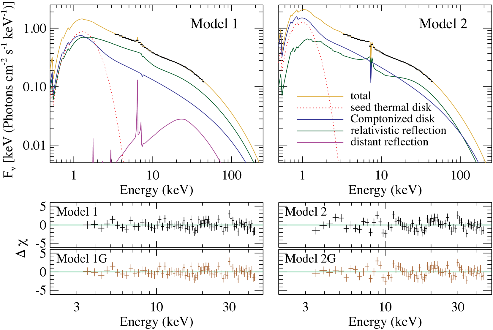
Figure 4.— A fully self-consistent model comprised of a Compton-scattered thermal disk component and associated reflection emission, as applied to the bright hard-state data of GX 339–4. The top panels show the composite fits and model components with the data in black. Model 1 is shown in left panels and Model 2 in the right. The $\sim$7.4 keV absorption line is evident in each, but is much more pronounced in Model 2. Bottom panels show the fit residuals for both self-consistent and non-self-consistent variants of each model. Note the similarity in the residuals among both variants for each of Models 1 and 2. The associated fits are presented in Table 1.

5. Results

Table 1GX 339–4 spectral fit results

Parameter	Prior	Model 1	Model 1G	Model 2	Model 2G
$\Gamma$	F	$1.65^{+0.01}_{-0.02}$	$1.583\pm 0.013$	$1.694\pm 0.011$	$1.662^{+0.004}_{-0.007}$
$f_{\rm sc}$	F	$0.42\pm 0.07$	$\cdots$	$0.32^{+0.09}_{-0.18}$	$\cdots$
$E_{\rm cut}$ (keV)	LF	$93.\pm 4.$	$88.\pm 3.$	$87.\pm 4.$	$90.\pm 3.$
$i$ (deg.)	F	$48.2\pm 1.2$	$48.2\pm 1.4$	$55.4^{+2.1}_{-1.6}$	$58.6^{+0.8}_{-1.1}$
$R_{\rm in}/R_{\rm ISCO}(a_{*}=0.998)$	F	$1.52_{-0.24}^{+0.18}$	$1.6_{-0.6}^{+0.2}$	$5.3\pm 0.8$	$1.4_{-0.3}^{+0.1}$
log $\xi$	F	$3.38^{+0.09}_{-0.05}$	$3.37^{+0.08}_{-0.05}$	$2.783\pm 0.017$	$2.803\pm 0.021$
$A_{\rm Fe}$ (solar)	LF	$6.3^{+1.8}_{-1.4}$	$7.8\pm 2.1$	$3.56\pm 0.20$	$4.0\pm 0.2$
$R_{\rm F}$	F	$0.8_{-0.2}^{+0.4}$	$0.206^{+0.016}_{-0.021}$	$0.75_{-0.08}^{+1.22}$	$0.492\pm 0.018$
$N_{\rm relxill}$	d,LF	$0.68\pm 0.12$	$1.36\pm 0.05$	$0.88_{-0.20}^{+0.43}$	$1.619\pm 0.022$
$kT_{\rm disk}$ (keV)	d	$0.31\pm 0.03$	$\cdots$	$0.15^{+0.05}_{-0.02}$	$\cdots$
$N_{\rm disk}$	d	$4300_{-1300}^{+2700}$	$\cdots$	$1.3^{+0.8}_{-0.6}\times 10^{5}$	$\cdots$
$N_{\rm xillver}$	LF	$0.28\pm 0.05$	$0.24\pm 0.03$	$\cdots$	$\cdots$
$E_{\rm gabs}$ (keV)	F	$7.38^{+0.16}_{-0.12}$	$7.39\pm 0.11$	$7.37\pm 0.04$	$7.45\pm 0.03$
$\tau_{\rm gabs}$	LF	$0.018\pm 0.005$	$0.019^{+0.006}_{-0.004}$	$0.154\pm 0.019$	$0.143\pm 0.015$
$L_{\rm ph}/L_{\rm ph,soft}$	F	$0.55\pm 0.10$	$\cdots$	$2.1^{+1.5}_{-0.5}$	$\cdots$
$\dot{M}/\dot{M}_{\rm soft}$	d	$0.40\pm 0.12$	$\cdots$	$4.1^{+5.4}_{-1.6}$	$\cdots$
$\chi^{2}/\nu$		69.65 / 59	68.21 / 59	113.82 / 60	105.46 / 60

Note. — All fits were explored using MCMC; values and errors represent maximum posterior-probability density and minimum-width 90% confidence intervals unless otherwise noted.

For each of Models 1 and 2, we contrast our self-consistent analyses of GX 339–4 against the “standard” reflection formalism as adopted in G15, i.e., a model with no self-consistent linking of disk and reflection/Compton components. To highlight their tie to the G15 paper, these comparison “standard” models are termed Models 1G and 2G.

In our analysis, we use XSPEC v12.9.0 (Arnaud, 1996) to perform a set of preliminary spectral fits. For consistency with G15, we employed relxill v0.2i, and we excluded the data in the first four channels while ignoring all data above 45 keV. To ensure that the redistribution of photons was accurately calculated, an extended logarithmic energy grid was employed that sampled from 1 eV to 1 MeV at 1.4% energy resolution via “energies 0.001 1000. 1000 log”. When a best fit was found, we estimate the errors through a rigorous exploration of parameter space carried out using Markov-Chain Monte Carlo (MCMC). We employed the python package emcee (Foreman-Mackey et al., 2013) as outlined in Steiner et al. (2012), with further details provided in Appendix C.

The corresponding results are summarized in Table 1, We present our best fits for both self-consistent models in Figure 4. The spectral components are shown as solid colored lines and the data are shown in black. The seed disk emission (i.e., the emission that would be observed from the bare disk if the corona were transparent) is shown as a red dotted line. The sharp cosmetic absorption line near Fe is strong and pronounced in Model 2, but suppressed by the xillver Fe-K$\beta$ edge in Model 1. Still, its inclusion in Model 1 is significant at a $\sim 5\leavevmode\nobreak\ \sigma$ level. Each of Models 1 and 2 produce relatively similar goodness-of-fits to their non-self-consistent counterparts and for both cases give nearly identical patterns of residuals as shown in the bottom panels. Thus, despite the constraints which result from regulating the interplay of the spectral components, our self-consistent framework very successfully models this extremely high-signal spectrum of GX 339–4 in its peak bright hard state.

As a result of imposing self-consistency, the low value of $R_{\rm F}$ obtained in G15 (i.e., Models 1G and 2G) has increased to several times its original value, now in a range close to unity which is aligned with expectation. In part, this increase occurs because the appreciable Comptonization by the corona ($f_{\rm SC}\sim 0.4$) dilutes the equivalent width of the Fe line (and other spectral features) since scattering a feature acts to blend it into the continuum (e.g., Steiner et al. 2016). Accordingly, in order for the (scattered) model to match the Fe-line strength in the data, $R_{\rm F}$ necessarily increases. This same effect was noted previously by Petrucci et al. (2001). For Model 1, surprisingly, the the best-fitting $R_{\rm in}$ decreased slightly relative to G15 (though within $\sim 1\sigma$ limits) by $\Delta R_{\rm in}\approx 0.1-0.2R_{\rm g}$. However, for Model 2 a new preferred solution emerges with an inner radius $R_{\rm in}$ that is $\sim 3.8$ times larger than for the non-self-consistent Model 2G.

We find that self-consistency does not ameliorate the problem of high Fe abundance, only slightly affecting its value. And based on the significantly better quality-of-fit for the Model 1 compared to Model 2, we conclude that the new self-consistent picture has not removed the need for two distinct reflection components. In fact, the $\chi^{2}$ gap between the two best fits is slightly larger for the self-consistent models.

Apart from the question of which model flavor performs best, there are several interesting differences between Models 1 and 2. For Model 2, because larger $R_{\rm in}$ is preferred, the self-consistent model is matched with correspondingly higher $N_{\rm disk}$ and lower $kT_{\rm disk}$. Model 2 also prefers lower values of the ionization parameter (by a factor of $\sim$ 5) and of $f_{\rm SC}$, but a higher inclination $i$. Most striking, the $\dot{M}$ required for Model 1 is less than half that of the reference, soft-state spectrum, whereas for Model 2, $\dot{M}$ is instead four-times larger that for the corresponding soft state!

Large $R_{\rm in}$ resulting in large $\dot{M}$ is a generic property of the self-consistent model because (from inspection of Eqns 4 and 5) if $R_{\rm in}$ is increased for a fixed $\dot{M}$, the photon flux diminishes and its peak moves to lower energy; both effects reduce the Compton power law’s amplitude. This is similar to the argument presented by Dovčiak & Done (2016) who detailed how the luminosity of the Compton component constrains the interplay between the seed photon flux and the corona’s covering factor. For a very luminous hard state (say, $\gtrsim 10\%$ of the Eddington limit), large-scale truncation ($R_{\rm in}>>R_{\rm ISCO}$) would imply highly super-Eddington values of $\dot{M}$.

To best examine the impact of the self-consistent model on the inner-radius (or equivalently, on the resulting spin determination), we present fit $\chi^{2}$ versus $R_{\rm in}$ in Figure 5. Here, solid lines show interpolations of “steppar” analyses in xspec (a routine which systematically optimizes the fit in sequential steps) across a range of $R_{\rm in}$. Overlaid as point-clouds are random samplings of the MCMC chains. For Models 1 and 2, it is evident that imposing self-consistency on the model has the effect of penalizing very low values of $R_{\rm in}$, and conversely making high $R_{\rm in}$ solutions more favorable. This effect does not significantly alter the best-fitting radius determined from Model 1, which significantly outperforms Model 2. However, self-consistency does alter the fit landscape, which is a clear indication that the self-consistent constraints can impact results.

In Model 2, which is statistically disfavored, the effect of self-consistency is much more pronounced: The $\chi^{2}$ surface is double-troughed, with one minimum at $R_{\rm in}\approx 1.4R_{\rm ISCO}$ (=1.8 $R_{g}$) and another at a much larger radius of $R_{\rm in}\approx 5.3R_{\rm ISCO}$ (=6.6 $R_{g}$). Thus, imposing self-consistency on Model 2 drastically changes the solution, favoring substantial truncation and penalizing mild truncation. The reason self-consistency produces this result is two-fold: (1) The downscattered Compton line emission contributes a flux excess in the same spectral region as the red wing of a relativistically-smeared line, and (2) the small-radius solution is penalized for requiring a disk component that is not observed. As can be gleaned from Figure 4, Models 1 versus 2 could readily be distinguished through direct detection of the thermal disk using a pile-up free detector with good low-energy sensitivity (e.g., NICER; Gendreau et al. 2012).

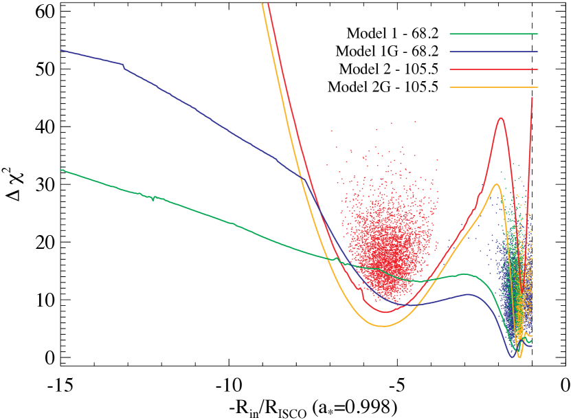
Figure 5.— The impact of a self-consistent paradigm on the determination of the inner-disk radius. We show the change in $\chi^{2}$ as the disk inner-radius is varied. The radius decreases to the right so that truncation is largest to the left. Model 1 is presented in green and Model 1G in blue; Model 2 is shown in red and Model 2G in orange. The clouds of points show random draws from the MCMC chains. Importantly, self-consistency penalizes small-radius solutions while reducing the penalty on truncated models. However, only for the disfavored Model 2 is the truncated disk preferred over the small-radius solution from G15 (i.e., Model 2G).

6. Discussion

Our results differ with those of Wilkins & Gallo (2015) concerning the effects of Comptonization on reflection in the inner disk. These authors find that strong Comptonization $f_{\rm SC}\gtrsim 0.5$ has the effect of reducing the breadth of line features emitted by the disk. The difference arises from their view of the corona as being centrally concentrated (though still porous) so that it very efficiently scatters emission from the inner disk where the gravitationally-broadened red wing is produced, while it is much less efficient at scattering emission from further out in the disk. We note that there is mixed evidence for a corona with this geometry; it is variously supported by microlensing data of distant quasars (e.g., Chartas et al. 2009) and reverberation studies which require very compact corona (Zoghbi et al., 2010), but it is contested by Dovčiak & Done (2016) on the grounds that a corona so compact would be starved of the seed photons required to produce the observed X-ray luminosity.

The contrast between the results of Wilkins & Gallo (2015) and ours highlights the importance of understanding coronal geometry and the necessity of investigating Compton-scattering effects for a range of geometries in order to better understand systematics in employing reflection spectroscopy to estimate disk radius and spin. At present, these matters are all but unexamined.

Basak & Zdziarski (2016) analyze XMM-Newton spectra of GX 339–4 using a model similar to ours, with the Compton, reflection and disk components modeled using nthcomp, relxill and a standard multicolor disk. While they cross-linked common parameters between the model components, a significant shortcoming of their approach is not tying the disk seed photons to the large number of photons scattered into the power law. They also did not account for Compton scattering of reflection emission in the corona. In contrast to our results, they found large-scale disk truncation, with $R_{\rm in}$ of tens of $R_{g}$, and they attributed a tentative detection of $\sim 0.2$ keV thermal emission to the thermalization of power-law photons in the disk’s atmosphere. Specifically, they claim $R_{\rm in}$ to be an order of magnitude larger than we find here. We note that if such large values of $R_{\rm in}$ are correct, then to produce the observed $1-10\leavevmode\nobreak\ \rm keV$ bright hard-state luminosity one would require the associated $\dot{M}$ to be extremely large, several times greater than the peak $\dot{M}$ of GX 339–4’s soft state. This is because for a given observed luminosity, when $R_{\rm in}$ is increased the disk photon luminosity and peak temperature for a given $\dot{M}$ both diminish. Both effects in turn cause the amplitude of the Compton power law to drop, and so match the data $\dot{M}$ must be large. If one makes the reasonable assertion that the soft state peaks close to the Eddington limit, then large-scale truncation $R>>R_{\rm ISCO}$ of a bright hard state would generally require a super-Eddington mass accretion rate.

Fürst et al. (2015) modeled low-luminosity hard-state NuSTAR spectra of GX 339–4. They found that the reflection component had a harder power-law index $\Gamma$ than the direct continuum component. The modest difference in the spectral indexes $\Delta\Gamma\approx 0.2-0.3$ is plausibly explained in our model by the hardening of the reflection spectrum due to Compton scattering in the corona. This can be readily seen in the dashed line of Fig. 3 which is harder than the input $\Gamma=2$. Although difficult to discern by eye in Figure 4, the Compton-scattered portion of the reflection component emerges from the corona with a harder spectral index, $\Delta\Gamma\approx 0.15$. This is because, like the Comptonized thermal photons, the Comptonized reflection spectrum is boosted in energy when scattering in the corona. As one would expect, the magnitude of $\Delta\Gamma$ can be shown to grow with $f_{\rm SC}$. This hardening explains why the reflection component can be brighter than the Compton continuum even if $R_{\rm F}<1$, as it quite apparently is for Model 1 in Figure 4. This occurs because the Compton-scattered reflection is effectively boosted by an additional factor of the “Compton y” parameter.

In applying our reflection model, we have proceeded under the assumption of maximal spin ($a_{*}=0.998$), which effectively sets $R_{\rm ISCO}$ for the thermal state data. If we had instead assumed any lower value for spin, the tension between the disk component (given that the data rule out a bright, hot disk) and reflection component (which prefers a disk proximate to the horizon) would have strictly increased, and the fits would have worsened. In this sense, our approach of adopting maximal spin provides a conservative estimate of the importance of self-consistency on the modeling.

7. Conclusions

In summary, we have demonstrated that the Comptonization of the Fe line and other reflection features in a hot corona can mimic the effects of relativistic distortion – and potentially affect estimates of black hole spin – by producing a downscattered red wing. This notionally calls into question the prevalence of dual-reflection component spectral models in which one component is in the relativistic domain, and hence strongly blurred, while the other one is assumed to occur far from the black hole and to be correspondingly narrow. The precise shape of a relativistically-distorted line is strongly affected by the spectral index, and hence it changes as a source transitions between hard and soft states. The Comptonization of reflection features is particularly important for hard spectral states because they are dominated by Compton-scattered photons from the thermal disk and their byproduct – reflection. Given that thermal disk photons are strongly Comptonized in hard states, the associated reflection emission is inevitably strongly Comptonized as well.

We have incorporated reflection and Comptonization into a self-consistent disk-coronal spectral model that properly conserves photons between the thermal, reflection, and Compton components. Within this framework, and using two specific models (Models 1 and 2), we analyzed a bright hard-state RXTE spectrum of GX 339–4 containing 44-million counts, which was analyzed previously by G15. An important constraint was obtained using a soft (thermal dominant) state spectrum of GX 339–4  at approximately the same luminosity as the G15 data to anchor $R_{\rm ISCO}$ and the hard-state disk scaling. From our analysis using the self-consistent models, we find that a single Compton-scattered reflection component is not preferred for GX 339–4; as in G15, the dual-reflection model is strongly favored. In fact, imposing self-consistency on the dual-reflection model and including the effects of Compton scattering on the broad reflection component has minor effect on the reflection best-fitting parameters aside from the reflection fraction $R_{\rm F}$ which is larger by a factor $\sim 2-4$. At the same time and importantly, the large change in the inner-disk radius for the disfavored Model 2 illustrates that self-consistency has the potential to significantly affect reflection estimates of black hole spin.

Additionally, we find that bright hard states cannot be reconciled with large-scale disk truncation unless either (1) the mass accretion rate $\dot{M}$ is super-Eddington (well in excess of the peak soft-state $\dot{M}$) or else (2) the hard state power-law component is attributed to another radiation mechanism. This conclusion is a consequence of the photon conservation that is a bedrock of our model. For a fixed $\dot{M}$ one can intuitively understand this result: a disk with large $R_{\rm in}$ is cool, produces few photons, and has a Compton component that peaks at lower energy. At the same time, the corona cannot be very small, or else it would require an enormously luminous disk to scatter sufficient photons into the observed power-law component.

For a multi-epoch study of a source, the effects of Compton scattering on reflection features can be assessed as the source ranges over soft and hard states; i.e., as the photon index $\Gamma$ varies. Our model predicts that any bias related to Compton scattering of the reflection emission having been omitted from modeling efforts should cause soft-state fits to measure lower spins than found in hard states for the same source (e.g., consistent with the findings of the most recent NuSTAR reflection studies of Cyg X–1).

As illustrated in Figure 5, enforcing self consistency has the potential to very significantly affect estimates of the inner disk radius and spin when modeling a reflection spectrum in the presence of a thermal component. Furthermore, this approach provides new, mutual constraints, e.g., on $R_{\rm in}$ and $\dot{M}$. Self-consistent reflection models therefore deserve exploration and further development.

Going forward, given that the power-law component in hard states is strongly Comptonized, standard practice should include Comptonization of the reflection component in the corona, particularly for studies aimed at constraining $R_{\rm in}$ or $a_{*}$.

Appendix A simplcomp

In addition to our adopted scattering kernel, which computes the photon redistribution following an exponentially cutoff power law, we have also implemented a kernel “comp” using the Comptonization model nthcomp to numerically compute the scattered distribution at each $E_{0}$. In xspec, toggling the energy turnover parameter positive or negative switches between kernels. A positive value calls comp (Życki et al., 1999; Zdziarski et al., 1996) and the value sets the electron temperature $kT_{e}$, whereas a negative value invokes Eqn. 1 and the absolute value of its setting gives $E_{\rm cut}$.

As evident in Figure 1, the kernels produce nearly identical profiles for the downscattered component, whereas the upscattered spectral shape is more sharply curved at its turnover using the physically rigorous comp kernel. We compare the fitting results obtained with both kernels in Table 2. Aside from the large value of $E_{\rm cut}/kT_{e}\sim 4-6$, the kernels produce similar results. The spectral index is slightly larger for the comp versus $E_{\rm cut}$ kernels for both Models 1 and 2. This is because the $E_{\rm cut}$ kernel overestimates the power-law curvature at energies well below the cutoff (as can be gleaned through close comparison between the kernel shapes in Fig. 1 at energies $\sim 2-50$ keV). This means that for the $E_{\rm cut}$ and comp kernels to match over the intermediate energy range below the turnover, an inherently steeper index is needed with comp.

Beyond the fits in Section 5, which aims to provide ready comparison with the results of G15, we have also explored the use of a new beta-version of relxill code which employs a nthcomp input continuum for reflection computations, as opposed to the cutoff power law. When applied in conjunction with the comp scattering kernel, this more physical continuum yields fits for each of Models 1 and 2 that are better than their counterparts in Tables 1 and 2. This bolsters the expectation that a physically accurate Comptonization model is preferred. A description of the nthcomp continuum implementation in relxill will be presented in future work.

Table 2GX 339–4 spectral fit comparison between $E_{\rm cut}$ and comp kernels

Parameter	Model 1 ($E_{\rm cut}$)	Model 1 (comp)		Model 2 ($E_{\rm cut}$)	Model 2 (comp)
$\Gamma$	$1.65^{+0.01}_{-0.02}$	$1.708\pm 0.015$		$1.694\pm 0.011$	$1.767^{+0.006}_{-0.013}$
$f_{\rm sc}$	$0.42\pm 0.07$	$0.44\pm 0.06$		$0.32^{+0.09}_{-0.18}$	$0.35^{+0.12}_{-0.18}$
$E_{\rm cut}{\rm\leavevmode\nobreak\ or\leavevmode\nobreak\ }kT_{e}$ (keV)	$93.\pm 4.$	$18.7^{+1.4}_{-1.0}$		$87.\pm 4.$	$19.9\pm 0.8$
$i$ (deg.)	$48.2\pm 1.2$	$48.6\pm 1.2$		$55.4^{+2.1}_{-1.6}$	$54.7\pm 1.4$
$R_{\rm in}/R_{\rm ISCO}(a_{*}=0.998)$	$1.52_{-0.24}^{+0.18}$	$1.40_{-0.13}^{+0.17}$		$5.3\pm 0.8$	$5.0\pm 0.7$
log $\xi$	$3.38^{+0.09}_{-0.05}$	$3.51^{+0.14}_{-0.09}$		$2.783\pm 0.017$	$2.776^{+0.019}_{-0.014}$
$A_{\rm Fe}$ (solar)	$6.3^{+1.8}_{-1.4}$	$9.7^{+0.2}_{-1.5}$		$3.56\pm 0.20$	$4.6\pm 0.3$
$R_{\rm F}$	$0.8_{-0.2}^{+0.4}$	$0.8_{-0.1}^{+0.5}$		$0.75_{-0.08}^{+1.22}$	$1.1_{-0.4}^{+1.3}$
$N_{\rm relxill}$	$0.68\pm 0.12$	$0.55^{+0.17}_{-0.04}$		$0.88_{-0.20}^{+0.43}$	$0.78_{-0.21}^{+0.45}$
$kT_{\rm disk}$ (keV)	$0.31\pm 0.03$	$0.31\pm 0.03$		$0.15^{+0.05}_{-0.02}$	$0.16^{+0.04}_{-0.02}$
$N_{\rm disk}$	$4300_{-1300}^{+2700}$	$4200_{-1100}^{+1400}$		$1.3^{+0.8}_{-0.6}\times 10^{5}$	$1.1^{+0.7}_{-0.4}\times 10^{5}$
$N_{\rm xillver}$	$0.28\pm 0.05$	$0.26\pm 0.07$		$\cdots$	$\cdots$
$E_{\rm gabs}$ (keV)	$7.38^{+0.16}_{-0.12}$	$7.35^{+0.13}_{-0.06}$		$7.37\pm 0.04$	$7.34\pm 0.03$
$\tau_{\rm gabs}$	$0.018\pm 0.005$	$0.030\pm 0.006$		$0.154\pm 0.019$	$0.174\pm 0.018$
$L_{\rm ph}/L_{\rm ph,soft}$	$0.55\pm 0.10$	$0.48^{+0.12}_{-0.04}$		$2.1^{+1.5}_{-0.5}$	$1.9^{+1.3}_{-0.4}$
$\dot{M}/\dot{M}_{\rm soft}$	$0.40\pm 0.12$	$0.34^{+0.12}_{-0.06}$		$4.1^{+5.4}_{-1.6}$	$3.3^{+4.3}_{-1.1}$
$\chi^{2}/\nu$	69.65 / 59	73.16 / 59		113.82 / 60	121.39/ 60

Note. — All fits were explored using MCMC; values and errors represent maximum posterior-probability density and minimum-width 90% confidence intervals unless otherwise noted.

Appendix B Deriving the disk’s scaling laws

Here, we present a concise derivation of the scaling laws employed for our self-consistent models, which relate the disk’s color temperature $T_{\rm col}$ and normalization $N$ to the disk inner radius $R_{\rm in}$ and photon luminosity $L_{\rm ph}$. Our prescription assumes that the hard state accretion disk is described by a standard thin-disk model (e.g., Shakura & Sunyaev 1973) down to $R_{\rm in}$. $R_{\rm in}$ can be as small as $R_{\rm ISCO}$, but if it is large then inward of $R_{\rm in}$ the disk is assumed to transition into a radiatively inefficient, geometrically thick and optically thin flow (e.g., as in the sequence described by Esin et al. 1997).

Allowing that the soft-state disk extends down to $R_{\rm in,soft}=R_{\rm ISCO}$, the ratio of hard-state and soft-state luminosities depends purely on the luminosity of each, and their respective efficiencies, $\eta\propto R^{-1}$. Recall that color temperature $T_{\rm col}=fT_{\rm eff}$ where $f\propto T_{\rm col}^{1/3}$, so $T_{\rm eff}\propto T_{\rm col}^{2/3}$. We adopt a simplifying notation where the lowercase letter indicates a dimensionless scaling for the hard-to-soft ratio. Specifically, $l\equiv\frac{L_{\rm hard}}{L_{\rm soft}}$, $r_{\rm in}\equiv\frac{R_{\rm in,hard}}{R_{\rm ISCO}}$, $\dot{m}\equiv\frac{\dot{M}_{\rm hard}}{\dot{M}_{\rm soft}}$, and $t\equiv\frac{T_{\rm hard}}{T_{\rm soft}}$. The luminosity,

$$l=\dot{m}r_{\rm in}^{-1}=r_{\rm in}^{2}t_{\rm eff}^{4}.$$ (B1)

The photon luminosity scales simply as the energy luminosity divided by the color temperature of the disk,

$$l_{\rm ph}=r_{\rm in}^{2}t_{\rm eff}^{4}t_{\rm col}^{-1}=r_{\rm in}^{2}t_{\rm col}^{5/3}.\\$$ (B2)

Equivalently, this yields a temperature scaling of

$$t_{\rm col}=l_{\rm ph}^{3/5}r_{\rm in}^{-6/5}.$$ (B3)

From Zimmerman et al. (2005), the disk normalization $N$ scales as $R_{\rm in}^{2}/f^{4}$. Here, we substitute the color temperature dependence of $f$, and define $n\equiv N_{\rm hard}/N_{\rm soft}$. Then,

$$n=r_{\rm in}^{2}t_{\rm col}^{-4/3}.$$ (B4)

Substituting the temperature scaling of Eqn B3, we obtain the scaling relation for normalization,

$$n=l_{\rm ph}^{-4/5}r_{\rm in}^{18/5}.$$ (B5)

Eqns B3 and B5 correspond to Eqns 2 and 3 in Section 5.

While the photon luminosity is a natural quantity for the examination of Comptonization, the more natural description of accretion employs $\dot{M}$. Combining Eqns B1 and B2 one finds,

$$l_{\rm ph}=\dot{m}t_{\rm col}^{-1}r_{\rm in}^{-1}=\dot{m}^{5/8}r_{\rm in}^{1/8}.$$ (B6)

Substituting Eqn B6 into Eqns B3 and  B5, one obtains

$$t_{\rm col}=\dot{m}^{3/8}r_{\rm in}^{-9/8},$$ (B7)

$$n=\dot{m}^{-1/2}r_{\rm in}^{7/2}.$$ (B8)

Appendix C MCMC run setup

The python emcee algorithm distributes a set of “walkers” that together explore the parameter landscape in a sequence of affine-invariant “stretch-move” steps. For our models, we used 50 walkers which were initially scattered about the point of the best fit and run for between 500,000 and 1,000,000 steps apiece. Our threshold for convergence was twenty auto-correlation lengths per walker in each parameter, corresponding to a minimum of 1,000 effective samplings. The associated computations were parallelized and the runs required approximately 2 CPU-years in aggregate. In the fits, as described in Steiner et al. (2012), each parameter was remapped using a logit transformation to regularize the space over which it was sampled from a finite interval to the real line, and each parameter was assigned a noninformative prior which was flat on either the parameter value, or on the logarithm of its value (for scale-independence).

References

- Arnaud (1996) Arnaud, K. A. 1996, in Astronomical Society of the Pacific Conference Series, Vol. 101, Astronomical Data Analysis Software and Systems V, ed. G. H. Jacoby & J. Barnes, 17
- Basak & Zdziarski (2016) Basak, R., & Zdziarski, A. A. 2016, MNRAS, 458, 2199
- Brenneman (2013) Brenneman, L. 2013, Measuring the Angular Momentum of Supermassive Black Holes
- Brenneman & Reynolds (2006) Brenneman, L. W., & Reynolds, C. S. 2006, ApJ, 652, 1028
- Chartas et al. (2009) Chartas, G., Kochanek, C. S., Dai, X., Poindexter, S., & Garmire, G. 2009, ApJ, 693, 174
- Chen et al. (2016) Chen, Z., Gou, L., McClintock, J. E., Steiner, J. F., Wu, J., Xu, W., Orosz, J., & Xiang, Y. 2016, ArXiv e-prints
- Coppi (1999) Coppi, P. S. 1999, in Astronomical Society of the Pacific Conference Series, Vol. 161, High Energy Processes in Accreting Black Holes, ed. J. Poutanen & R. Svensson, 375–+
- Coriat et al. (2011) Coriat, M., et al. 2011, MNRAS, 414, 677
- Dauser et al. (2014a) Dauser, T., García, J., Parker, M. L., Fabian, A. C., & Wilms, J. 2014a, MNRAS, 444, L100
- Dauser et al. (2014b) —. 2014b, MNRAS, 444, L100
- Dauser et al. (2016) Dauser, T., García, J., Walton, D. J., Eikmann, W., Kallman, T., McClintock, J., & Wilms, J. 2016, A&A, 590, A76
- Davis & Hubeny (2006) Davis, S. W., & Hubeny, I. 2006, ApJS, 164, 530
- Dovčiak & Done (2016) Dovčiak, M., & Done, C. 2016, Astronomische Nachrichten, 337, 441
- Dovčiak et al. (2004) Dovčiak, M., Karas, V., & Yaqoob, T. 2004, ApJS, 153, 205
- Esin et al. (1997) Esin, A. A., McClintock, J. E., & Narayan, R. 1997, ApJ, 489, 865
- Fabian et al. (1989) Fabian, A. C., Rees, M. J., Stella, L., & White, N. E. 1989, MNRAS, 238, 729
- Fabian & Ross (2010) Fabian, A. C., & Ross, R. R. 2010, Space Sci. Rev., 157, 167
- Foreman-Mackey et al. (2013) Foreman-Mackey, D., Hogg, D. W., Lang, D., & Goodman, J. 2013, PASP, 125, 306
- Fuerst et al. (2016) Fuerst, F., et al. 2016, ArXiv e-prints
- Fürst et al. (2015) Fürst, F., et al. 2015, ApJ, 808, 122
- García et al. (2014) García, J., et al. 2014, ApJ, 782, 76
- García & Kallman (2010) García, J., & Kallman, T. R. 2010, ApJ, 718, 695
- García et al. (2015) García, J. A., Steiner, J. F., McClintock, J. E., Remillard, R. A., Grinberg, V., & Dauser, T. 2015, ApJ, 813, 84, (G15)
- Gendreau et al. (2012) Gendreau, K. C., Arzoumanian, Z., & Okajima, T. 2012, in Proc. SPIE, Vol. 8443, Space Telescopes and Instrumentation 2012: Ultraviolet to Gamma Ray, 844313
- Gierliński et al. (1999) Gierliński, M., Zdziarski, A. A., Poutanen, J., Coppi, P. S., Ebisawa, K., & Johnson, W. N. 1999, MNRAS, 309, 496
- Gou et al. (2011) Gou, L., et al. 2011, ApJ, 742, 85
- Haardt & Maraschi (1993) Haardt, F., & Maraschi, L. 1993, ApJ, 413, 507
- Jahoda et al. (2006) Jahoda, K., Markwardt, C. B., Radeva, Y., Rots, A. H., Stark, M. J., Swank, J. H., Strohmayer, T. E., & Zhang, W. 2006, ApJS, 163, 401
- Kubota & Done (2016) Kubota, A., & Done, C. 2016, MNRAS, 458, 4238
- Li et al. (2005) Li, L.-X., Zimmerman, E. R., Narayan, R., & McClintock, J. E. 2005, ApJS, 157, 335
- Matt et al. (1997) Matt, G., Fabian, A. C., & Reynolds, C. S. 1997, MNRAS, 289, 175
- McClintock et al. (2014) McClintock, J. E., Narayan, R., & Steiner, J. F. 2014, Space Sci. Rev., 183, 295
- Miller et al. (2009) Miller, J. M., Reynolds, C. S., Fabian, A. C., Miniutti, G., & Gallo, L. C. 2009, ApJ, 697, 900
- Parker et al. (2016) Parker, M. L., et al. 2016, ApJ, 821, L6
- Parker et al. (2015) —. 2015, ApJ, 808, 9
- Peris et al. (2016) Peris, C. S., Remillard, R. A., Steiner, J. F., Vrtilek, S. D., Varnière, P., Rodriguez, J., & Pooley, G. 2016, ApJ, 822, 60
- Petrucci et al. (2001) Petrucci, P. O., Merloni, A., Fabian, A., Haardt, F., & Gallo, E. 2001, MNRAS, 328, 501
- Plant et al. (2015) Plant, D. S., Fender, R. P., Ponti, G., Muñoz-Darias, T., & Coriat, M. 2015, A&A, 573, A120
- Poutanen & Svensson (1996) Poutanen, J., & Svensson, R. 1996, ApJ, 470, 249
- Pozdnyakov et al. (1983) Pozdnyakov, L. A., Sobol, I. M., & Syunyaev, R. A. 1983, Astrophysics and Space Physics Reviews, 2, 189
- Remillard & McClintock (2006) Remillard, R. A., & McClintock, J. E. 2006, ARA&A, 44, 49
- Reynolds (2014) Reynolds, C. S. 2014, Space Sci. Rev., 183, 277
- Shakura & Sunyaev (1973) Shakura, N. I., & Sunyaev, R. A. 1973, A&A, 24, 337
- Steiner et al. (2010) Steiner, J. F., McClintock, J. E., Remillard, R. A., Gou, L., Yamada, S., & Narayan, R. 2010, ApJ, 718, L117
- Steiner et al. (2009a) Steiner, J. F., McClintock, J. E., Remillard, R. A., Narayan, R., & Gou, L. J. 2009a, ApJ, 701, L83
- Steiner et al. (2009b) Steiner, J. F., Narayan, R., McClintock, J. E., & Ebisawa, K. 2009b, PASP, 121, 1279
- Steiner et al. (2012) Steiner, J. F., et al. 2012, MNRAS, 427, 2552
- Steiner et al. (2011) —. 2011, MNRAS, 416, 941
- Steiner et al. (2016) Steiner, J. F., Remillard, R. A., García, J. A., & McClintock, J. E. 2016, ApJ, 829, L22
- Titarchuk (1994) Titarchuk, L. 1994, ApJ, 434, 570
- Tomsick et al. (2014) Tomsick, J. A., et al. 2014, ApJ, 780, 78
- Walton et al. (2016) Walton, D. J., et al. 2016, ApJ, 826, 87
- White & Holt (1982) White, N. E., & Holt, S. S. 1982, ApJ, 257, 318
- Wilkins & Gallo (2015) Wilkins, D. R., & Gallo, L. C. 2015, MNRAS, 448, 703
- Wilms et al. (2000) Wilms, J., Allen, A., & McCray, R. 2000, ApJ, 542, 914
- Zdziarski et al. (1996) Zdziarski, A. A., Johnson, W. N., & Magdziarz, P. 1996, MNRAS, 283, 193
- Zhang et al. (1997) Zhang, S. N., Cui, W., & Chen, W. 1997, ApJ, 482, L155
- Zimmerman et al. (2005) Zimmerman, E. R., Narayan, R., McClintock, J. E., & Miller, J. M. 2005, ApJ, 618, 832
- Zoghbi et al. (2010) Zoghbi, A., Fabian, A. C., Uttley, P., Miniutti, G., Gallo, L. C., Reynolds, C. S., Miller, J. M., & Ponti, G. 2010, MNRAS, 401, 2419
- Życki et al. (1999) Życki, P. T., Done, C., & Smith, D. A. 1999, MNRAS, 309, 561