Elastic collision and molecule formation of spatiotemporal light bullets in a cubic-quintic nonlinear medium

Abstract

We consider the statics and dynamics of a stable, mobile three-dimensional (3D) spatiotemporal light bullet in a cubic-quintic nonlinear medium with a focusing cubic nonlinearity above a critical value and any defocusing quintic nonlinearity. The 3D light bullet can propagate with a constant velocity in any direction. Stability of the light bullet under a small perturbation is established numerically. We consider frontal collision between two light bullets with different relative velocities. At large velocities the collision is elastic with the bullets emerge after collision with practically no distortion. At small velocities two bullets coalesce to form a bullet molecule. At a small range of intermediate velocities the localized bullets could form a single entity which expands indefinitely leading to a destruction of the bullets after collision. The present study is based on an analytic Lagrange variational approximation and a full numerical solution of the 3D nonlinear Schrödinger equation.

I Introduction

A bright soliton is a self-bound object that travels at a constant velocity in one dimension (1D), due to a cancellation of nonlinear attraction and defocusing forces book ; sol . The 1D soliton in a cubic Kerr medium has been observed in nonlinear optics book ; sol and in Bose-Einstein condensates rmp . Specifically, optical temporal temporal and spatial 1996 solitons were observed for a cubic Kerr nonlinearity. However, a three-dimensional (3D) spatiotemporal soliton cannot be formed in isolation with a cubic Kerr nonlinearity due to collapse collapse ; book . The same is true about a two-dimensional (2D) spatial soliton with a Kerr nonlinearity. However, the solitons can be stabilized in higher dimensions for a saturable lbth ; collapse or a modified nonlinearity quartic , or by a nonlinearity sadhan or dispersion sadhan2 management among other possibilities malomed ; malomed2 . A 2D spatiotemporal optical soliton has been observed stempo in a saturable nonlinearity generated by the cascading of quadratic nonlinear processes. The generation of a 2D spatial soliton in an attractive cubic and repulsive quintic medium has been suggested 2dcqth and realized experimentally 2dcqexp . The generation of a stable 2D vortex soliton in a cubic-quintic medium has been suggested 2dcqvor .

Light bullets collapse are localized 3D pulses of electromagnetic energy that can travel through a medium and retain their spatiotemporal shape due to a balance between the non-linear self-focusing and spreading effects of the medium in which the pulse beam propagates. Such light bullets are unstable and collapse in a cubic Kerr medium. Light bullets were realized experimentally in arrays of wave guides lbexp . There were many theoretical $-$ numerical and analytical $-$ studies which established robustness and approximate solitonic nature of the light bullets using the 3D nonlinear Schrödinger (NLS) equation book with a modified nonlinearity quartic ; lbth , dissipation gl , and/or dispersion sadhan2 . A saturable nonlinearity leads to stable optical bullets lbth . Nonlinear dissipation in the complex cubic-quintic Ginzburg-Landau equation also stabilizes the bullets gl . Dispersion management can stabilize light bullets in a medium with cubic nonlinearity boris1 . There has been variational study of light bullets in a cubic-quintic medium cq where a condition of stability was obtained. Another study suggested a way of the stabilization of light bullets in a cubic-quintic medium by a periodic variation of diffraction and dispersion stacq .

In this paper we study the formation of a 3D spatiotemporal light bullet lbth ; collapse in a cubic-quintic medium for a defocusing quintic nonlinearity and a focusing cubic nonlinearity as the ground state of the 3D NLS equation. A cubic-quintic medium is of experimental interest also. The study with a polydiacetylene paratoluene sulfonate crystal in the wavelength region near 1600 nm shows that the refractive index versus input intensity correlation leads to a cubic-quintic form of nonlinearity in the NLS equation book ; cqexpt . The cubic-quintic nonlinearity also arises in a low intensity expansion of the saturable nonlinearity used in the pioneering study of light bullets lbth . In this study of light bullets in a cubic-quintic medium we find that a stable light bullet can be formed for the cubic focusing nonlinearity above a critical value in the 3D NLS equation for any finite quintic defocusing nonlinearity. The statical properties of the light bullet is studied using a Lagrange variational analysis and a complete numerical solution of the 3D NLS equation. The variational and numerical results are found to be in good agreement with each other. The stability of the light bullet is established numerically under a small perturbation introduced by changing the cubic nonlinearity by a small amount, while the bullet is found to execute sustained breathing oscillation.

The light bullet can move freely without deformation along any direction with a constant velocity. We also study the frontal collision between two light bullets. Only the collision between two integrable 1D solitons is truly elastic book . As the dimensionality of the soliton is increased such collision is expected to become inelastic with loss of energy in 2D and 3D. In the present numerical simulation of frontal collision between two light bullets in different parameter domains of nonlinearities and velocities three distinct scenarios are found to take place. At sufficiently large velocities the collision is found to be quasi elastic when the two bullets emerge after collision with practically no deformation. At small velocities the collision is inelastic and the bullets form a single bound entity in an excited state and last for ever and execute oscillation. We call this a bullet molecule. In a small domain of intermediate velocities, the bullets coalesce to form a single entity, which expands indefinitely leading to the destruction of the bullets.

.

We present the 3D NLS equation used in this study in Sec. II. In Sec. III we present the numerical results for stationary profiles of 3D spatiotemporal light bullets. We present numerical tests of stability of the light bullet under a small perturbation. The quasi-elastic nature of collision of two solitons at large velocities and bullet molecule formation at low velocities are demonstrated by real-time simulation. We end with a summary of our findings in Sec. IV.

II Nonlinear Schrödinger equation: Variational formulation

In nonlinear fibre optics a general 3D NLS equation can usually be written as book ; agarwal

$$\,{\Big{[}}i\frac{\partial}{\partial z}+\frac{1}{2\beta_{0}}\nabla_{\perp}^{2}+\frac{\beta_{2}}{2}\frac{\partial^{2}}{\partial\mathrm{t}^{2}}+\gamma|A|^{2}{\Big{]}}A(\mathrm{x,y,t})=0,$$ (1)

$$\nabla_{\perp}^{2}=\frac{\partial^{2}}{\partial\mathrm{x}^{2}}+\frac{\partial^{2}}{\partial\mathrm{y}^{2}},$$ (2)

where $\beta_{2}$ is dispersion parameter and can be positive or negative with magnitude of the order of 10${}^{-3}\sim 10^{-2}$ ps²/m agarwal , the nonlinear parameter $\gamma$ has unit $W^{-1}$m, the unit of $|A|^{2}$ is $W$m^-2, $\beta_{0}=2\pi n_{0}/\lambda$ is the propagation parameter book , where $n_{0}$ is the refractive index and $\lambda$ is the wave length of the beam. The function $A$ describes the evolution of the beam envelop. For a spatiotemporal soliton it is useful to define the characteristic lengths for dispersion $L_{DS}\equiv\tau^{2}/|\beta_{2}|$, and diffraction $L_{DF}\equiv 2n_{0}\pi\rho^{2}/\lambda$ where $\rho$ is the radius of the beam, and $\tau$ is the time scale of the soliton malomed . For an equilabrated propagation of the spatiotemporal soliton these two lengths are to be equal $-$ $L_{DS}=L_{DF}\equiv L_{D}$ $-$ yielding $\rho^{2}=L_{D}\lambda/({2\pi n_{0}}).$ Now by scaling we define the following dimensionless variables agarwal

$$\;x=\frac{\mathrm{x}}{\rho},\;y=\frac{\mathrm{y}}{\rho},\;t=\frac{\mathrm{t}}{\tau},\;z=\frac{\mathrm{z}}{L_{D}},\;{\phi=\frac{A\rho}{\sqrt{P}_{0}},\;p=\frac{\gamma P_{0}L_{D}}{\rho^{2}}.}$$ (3)

The scale $P_{0}$ is chosen, so that $\int|\phi|^{2}dxdydt=1.$ Using the dimensionless variables we obtain the following dimensionless NLS equations with self-focusing cubic and self-defocusing quintic nonlinearity book

$$\,{\Big{[}}i\frac{\partial}{\partial z}+\frac{1}{2}\left(\frac{\partial^{2}}{\partial x^{2}}+\frac{\partial^{2}}{\partial y^{2}}+\frac{\partial^{2}}{\partial t^{2}}\right)+p|\phi|^{2}-q|\phi|^{4}{\Big{]}}\phi({\bf r},z)=0,$$ (4)

in scaled units where ${\bf r}\equiv\{x,y,t\}$, $p$ is the cubic and $q$ the quintic nonlinearity. Here $z$ is the propagation distance, $x,y$ denote transverse extensions, and $t$ the time. The plus sign before $|\phi|^{2}$ in Eq. (4) denotes a self-focusing cubic nonlinearity. The quintic nonlinearity of strength $q$ with a negative sign denote self-defocusing.

To have an idea of the length and time scales concerned, let us consider the case of an infrared beam of wave length $\lambda=1$ $\mu$m, and take a nonlinear medium of $\beta_{2}=10^{-2}$ ps²/m, and a time scale $\tau=60$ fs. Then the propagation length $L_{D}=36$ cm and the beam width $\rho\approx 239$ $\mu$m. These numbers are quite similar to those in an experiment on spatiotemporal soliton in a planar glass waveguide sptex . In this paper we quote the results in dimensionless units, which can be easily converted to actual experimental units following these guidelines.

For an analytic understanding we consider the Lagrange variational formulation of the formation of a light bullet. In this spherically symmetric problem, convenient analytic Lagrangian variational approximation of Eq. (4) can be obtained with the following Gaussian ansatz for the wave function pg

$$\phi({\bf r},z)=\frac{\pi^{-3/4}}{w^{3/2}(z)}\exp\left[-\frac{r^{2}}{2w^{2}(z)}+i\alpha(z)r^{2}\right],$$ (5)

where $r^{2}=x^{2}+y^{2}+t^{2}$, $w(z)$ is the width and $\alpha(z)$ is the chirp. The Lagrangian density corresponding to Eq. (4) is given by

$${\cal L}({\bf r},z)=\frac{i}{2}\left[\phi({\bf r},z)\frac{\partial\phi^{*}({\bf r},z)}{\partial z}-\phi^{*}({\bf r},z)\frac{\partial\phi({\bf r},z)}{\partial z}\right]$$

$$+\frac{|\nabla\phi({\bf r},z)|^{2}}{2}-\frac{p}{2}|\phi({\bf r},z)|^{4}+\frac{q}{3}|\phi({\bf r},z)|^{6}.$$ (6)

Consequently, the effective Lagrangian $L\equiv\int{\cal L}({\bf r},z)d{\bf r}$ becomes

$$L=\frac{3}{2}w^{2}\dot{\alpha}+\frac{3}{4w^{2}}+3w^{2}\alpha^{2}-\frac{p\pi^{-3/2}}{4\sqrt{2}w^{3}}+\frac{q\pi^{-3}}{9\sqrt{3}w^{6}},$$ (7)

where the overhead dot denotes the $z$ derivative. The actual physical dimension J/m of this dimensionless Lagrangian $L$ can be restored upon multiplication by the factor $\tau P_{0}/L_{D}$. The Euler-Lagrange equation for this Lagrangian yields the following ordinary differential equation for the width $w$:

$$\ddot{w}=\frac{1}{w^{3}}-\frac{p(2\pi)^{-3/2}}{w^{4}}+\frac{4q\pi^{-3}}{9\sqrt{3}w^{7}}.$$ (8)

The energy of the stationary bullet is the Lagrangian (7) with $\alpha=0$, e. g.,

$$E=\frac{3}{4w^{2}}-\frac{p\pi^{-3/2}}{4\sqrt{2}w^{3}}+\frac{q\pi^{-3}}{9\sqrt{3}w^{6}}.$$ (9)

The width $w$ of a stationary bullet is obtained by setting the right-hand-side of Eq. (8) to zero:

$$\frac{1}{w^{3}}-\frac{p(2\pi)^{-3/2}}{w^{4}}+\frac{4q\pi^{-3}}{9\sqrt{3}w^{7}}=0,$$ (10)

which is the condition for a minimum of energy $E$ $-$ $dE/dw=0,d^{2}E/dw^{2}>0$ . Without the quintic term ($q=0$) the bullet of width $w=p/(2\pi)^{3/2}$ is tantamount to an unstable Towne’s soliton towne . We will demonstrate that for stability a non-zero quintic term ($q\neq 0$) is necessary. For $q>0$, Eq. (10) has solution for the cubic nonlinearity $p$ above a critical value $p_{\mathrm{crit}}$, which is the threshold for the formation of the bullet.

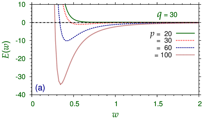
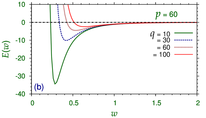
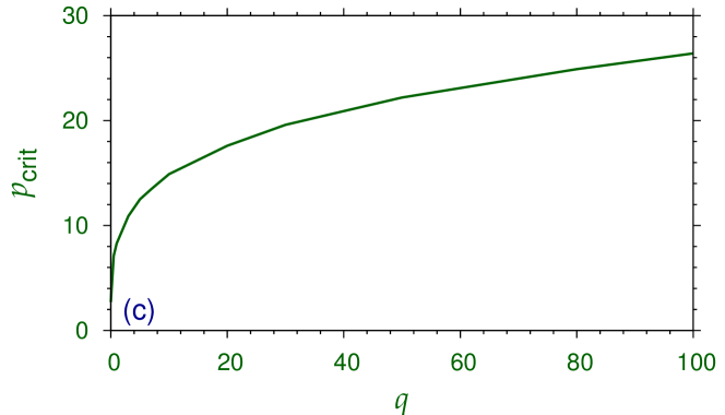
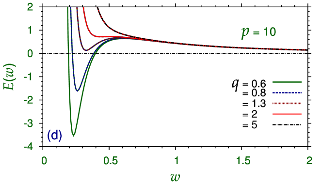
Figure 1: (Color online) (a) Variational energy versus width ($E-w$) plot for different cubic nonlinearities $p(=20,30,60,100)$ and quintic nonlinearity $q=30.$ (b)The same for different quintic nonlinearities $q$ $(=10,30,60,100)$ and cubic nonlinearity $p=60.$ (c) Variational critical cubic nonlinearity $p_{\mathrm{crit}}$ for light bullet formation, obtained from Eq. (10), for different values of quintic nonlinearity $q$. (d) Variational energy versus width ($E-w$) plot for different quintic nonlinearities $q(=0.6,0.8,1.3,2,5)$ and cubic nonlinearity $p=10.$

III Numerical Results

Unlike in the 1D case, the 3D NLS equation (4) does not have analytic solution and different numerical methods, such as split-step Crank-Nicolson CPC and Fourier spectral jpb methods, are used for its solution. Here we solve it numerically by the split-step Crank-Nicolson method in Cartesian coordinates using a $\bf r$ $=\{x,y,t\}$ step of $0.025$ and a $z$ step of $0.0002$ CPC . The number of ${\bf r}$ discretization points for each components is 256. There are different C and FORTRAN programs for solving the NLS-type equations CPC ; CPC1 and one should use the appropriate one. We use both imaginary- and real-$z$ propagations CPC in the numerical solution of the 3D NLS equation. The imaginary-$z$ propagation is appropriate to find the stationary lowest-energy profile of the bullet. This method replaces $z$ by a new variable $\hat{z}\equiv iz$ and consequently Eq. (4) becomes completely real and a $z$-iteration of this equation leads to the lowest-energy state with high accuracy. The real-$z$ propagation involve complex variable and hence is more complicated and less accurate. However, the real-$z$ propagation yields the propagation dynamics of the bullet. In the imaginary-$z$ propagation, as the propagation variable $z$ is replaced by the (unphysical) variable $\hat{z}$, this method cannot lead to the propagation dynamics of the bullet. In the imaginary-$z$ propagation the initial state was taken as in Eq. (5) with $\alpha(z)=0$ and the width $w$ set equal to the variational solution obtained by solving Eq. (10). The convergence will be quick if the guess for the width $w$ is close to the final width. All stationary profiles of the bullets are calculated by imaginary-$z$ propagation. The dynamics and collision are then studied by real-$z$ propagation using the initial profile obtained in the imaginary-$z$ propagation.

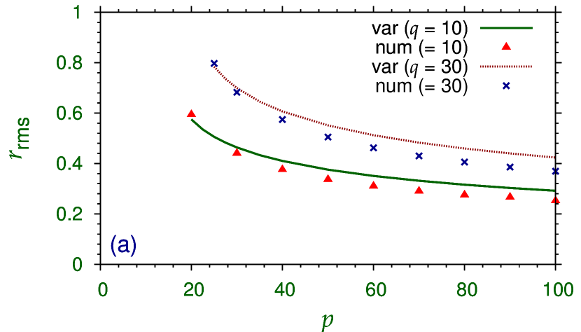
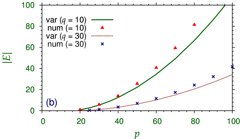
Figure 2: (Color online) Variational (var) and numerical (num) (a) rms radius and (b) energy $|E|$ versus cubic nonlinearity $p$ of a light bullet for two different quintic nonlinearities $q$ $(=10,30)$.

The stable bullet corresponds to an energy ($E$) minimum as given by Eq. (10). In Figs. 1(a) and (b) we plot $E$ versus $w$ of Eq. (10) for different cubic ($p$) and quintic ($q$) nonlinearities. The energy minima of these plots correspond to a stable bullet of negative energy. From Fig. 1(a) we find that for $q=30$ such an energy minima exists for $p>20$. An accurate value of this limit can be obtained from Eq. (10): for $q=30$ this equation has solution for $p\geq p_{\mathrm{crit}}=19.6$. Hence the NLS equation (4) can have a stable light bullet solution for cubic nonlinearity $p$ greater than a critical value $p_{\mathrm{crit}}$. For $p<p_{\mathrm{crit}}$ the system is much too repulsive and is not bound and escapes to infinity. However, this critical value $p_{\mathrm{crit}}$ of $p$ is a function of the quintic nonlinearity $q$. The $p_{\mathrm{crit}}-q$ correlation can be found from an attempt to solve Eq. (10) numerically. The $p_{\mathrm{crit}}-q$ correlation obtained in this fashion is plotted in Fig. 1(c). However, in addition to these stable bullets corresponding to a global minimum of energy with negetive energy values, one can also have metastable bullets corresponding to a local minimum of energy at positive energies. Such a situation is illustrated in Fig. 1(d) where we plot the variational $E-w$ curves for $p=10$ and different $q$ values. The bullet with $p=10$ and $q=1.3$ has a local minimum at a positive energy and is metastable in nature. In the following we will only consider the stable light bullets with negative energy.

Next we compare in Fig. 2(a) the numerical and variational root-mean-square (rms) radius $r_{\mathrm{rms}}$ of a light bullet versus cubic nonlinearity $p$ for different quintic nonlinearity $q=10,30$. The variational result is given by: $r_{\mathrm{rms}}=\sqrt{3/2}{w}$, where $w$ is the equilibrium variational width. In Fig. 2(b) we show the numerical and variational energy $|E|$ of a light bullet versus $p$ for different $q$. The numerical energy is calculated using Eq. (9) with the numerically obtained $\phi({\bf r},z)$. The energy of the light bullet is negative in all cases and its absolute value is plotted. For small $p$, the agreement between numerical and variational results is better. For large $p$, the agreement between the two is qualitative. For large nonlinearity $p$ in the NLS equation, the profile of the bullet deviates more from the Gaussian variational ansatz $-$ thus making the variational results more approximate.

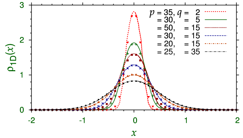
Figure 3: (Color online) Numerical (line) and variational (chain of symbols) reduced 1D density $\rho_{1D}(x)$ for different cubic nonlinearity $p$ and quintic nonlinearity $q$.

To study the density distribution of the light bullets we calculate the reduced 1D density defined by

$$\rho_{\mathrm{1D}}(x)=\int dtdy|\phi({\bf r})|^{2}.$$ (11)

In Fig. 3 we plot this reduced 1D density as obtained from variational and numerical calculations for different cubic nonlinearity $p$ and quintic nonlinearity $q$. For a fixed defocusing nonlinearity $q$ $(=15)$, the light bullet is more compact with the increase of focusing nonlinearity $p$ resulting in more attraction. For a fixed focusing nonlinearity $p$ $(=20)$, the light bullet is more compact with the decrease of defocusing nonlinearity $q$ resulting in less repulsion.

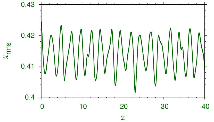
Figure 4: (Color online) Steady oscillation of the rms size $x_{\mathrm{rms}}$ during real-$z$ propagation of a light bullet with $p=20$ and $q=15$, when at $z=0$ the cubic nonlinearity $p$ is suddenly changed from 20 to 20.5.

Now we present a numerical test of stability of a stable bullet under a small perturbation. For this purpose we consider the bullet shown in Fig. 3 with $p=20$ and $q=15$ as calculated by imaginary-$z$ propagation. Using the imaginary-$z$ profile as the initial state we perform numerical simulation by real-$z$ propagation under a small perturbation introduced at $z=0$ by changing $p$ from 20 to 20.5. This sudden perturbation in the cubic nonlinearity increases the attraction in the system and the light bullet starts a rapid breathing oscillation. In Fig. 4 we show the steady oscillation in the rms $x$ size $x_{\mathrm{rms}}$ versus propagation distance $z$ during real-$z$ propagation. The steady continued oscillation of the bullet over a long distance of propagation establishes the stability of the bullet. The real-$z$ simulation was performed in full 3D space without assuming spherical symmetry to guaranty the stability in full 3D Cartesian space.

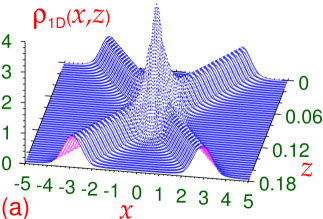
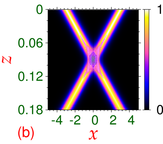
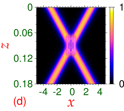
Figure 5: (Color online) (a) The 1D density $\rho_{1D}(x,z)$ and (b) its contour plot during the collision of two light bullets of Fig. 3 with $p=20,q=15$ initially placed at $x=\pm 3$ , upon real-$z$ propagation. The initial wave functions are multiplied by $\exp(\pm i40x)$ which sets them in motion with velocity of about $33$ each. The same for two light bullets with $p=25,q=35$ of Fig. 3 are shown in (c) and (d).

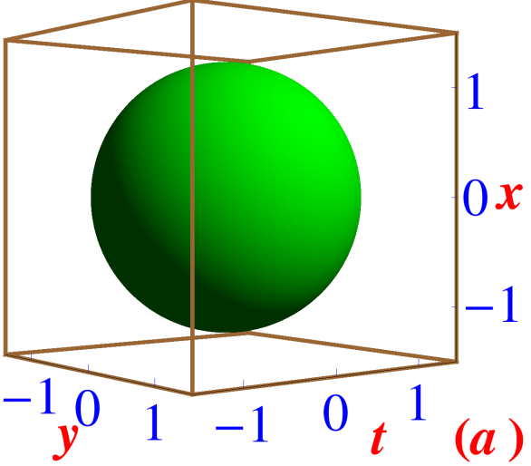
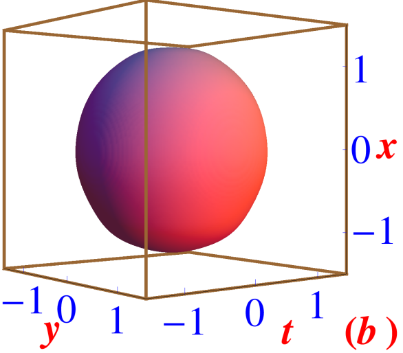
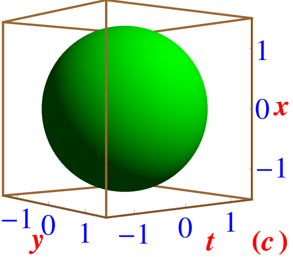
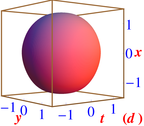
Figure 6: (Color online) 3D isodensity profile of the (a) initial (at $z=0$) and (b) final (at $z=0.18$) light bullets each with $p=20,q=15$ and (c) initial (at $z=0$) and (d) final (at $z=0.18$) light bullets each with $p=25,q=35$ undergoing elastic collision illustrated in Fig. 5(a) and (b). density on contour 0.01.

The collision between two analytic 1D solitons is truly elastic rmp ; book and such solitons pass through each other without deformation at any incident velocities. The collision between two 3D spatiotemporal light bullets is expected to be inelastic in general with loss of kinetic energy resulting in the deformation of the bullets. Such a collision can at best be quasi-elastic. To test the solitonic nature of the present light bullets, we study the frontal head-on collision of two bullets. The imaginary-$z$ profiles of the light bullets shown in Fig. 3 with (i) $p=20,q=15$ and (ii) $p=25,q=35$ are used as the initial function in the real-$z$ simulation of collision, with two identical bullets placed at $x=\pm 3$ initially for $z=0$. To set the light bullets in motion along the $x$ axis in opposite directions the respective wave functions are multiplied by $\exp(\pm i40x)$. To illustrate the dynamics upon real-$z$ simulation, we plot the time evolution of 1D density $\rho_{1D}(x,z)\equiv\int dt\int dy|\phi({\bf r},z)|^{2}$ in Fig. 5(a) for the collision of two bullets with $p=20,q=15$. The corresponding contour plot is presented in Fig. 5(b). The same for the collision of two light bullets with $p=25,q=35$ is presented in Figs. 5(c) and (d). The dimensionless velocity of a light bullet is about 33 and the deviation from elastic collision is found to be small. Considering the three-dimensional nature of collision, the distortion in the bullet profile is found to be negligible. To visualize the amount of inelasticity in the collision displayed in Figs. 5(a) and (b), we display in Figs. 6(a) and (b) the 3D isodensity profile of the light bullet before ($z=0$) and after ($z=0.18$) the collision shown in Figs. 5(a) and (b). The same for the collision shown in Figs. 5(c) and (d) is illustrated in Figs. 6(c) and (d). In general, the inelasticity in both collisions is small.

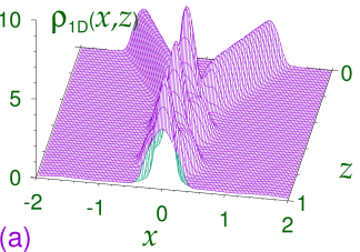
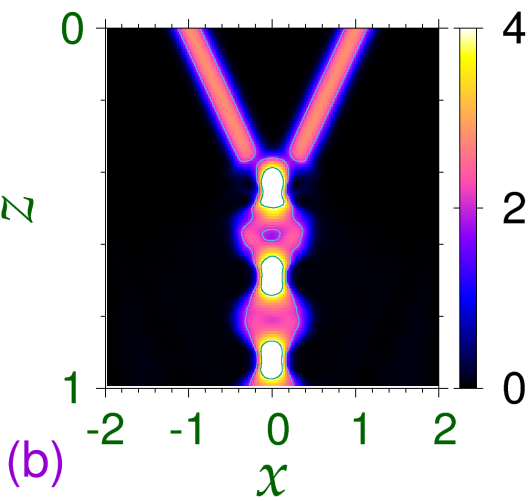
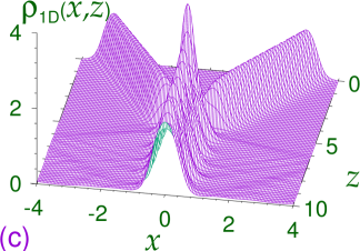
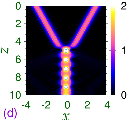
Figure 7: (Color online) (a) The 1D density $\rho_{1D}(x,z)$ and (b) its contour plot during the collision of two light bullets of Fig. 3 with $p=35,q=2$ initially placed at $x=\pm 1$, upon real-$z$ propagation. The initial wave functions are multiplied by $\exp(\pm i2x)$ to set them in motion with an initial dimensionless velocity of about 2. The same for the collision of two light bullets with $p=30,q=15$ of Fig. 3 for an initial velocity of about $0.5$ are shown in (c) and (d), respectively.

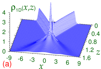
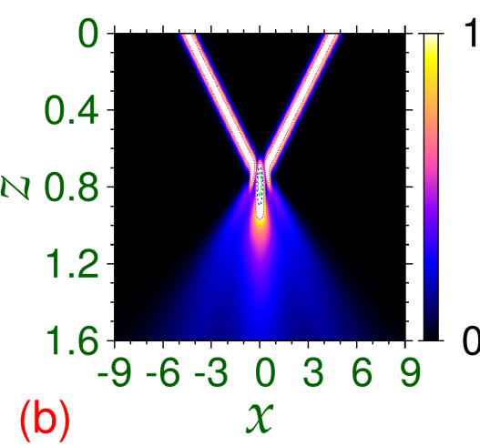
Figure 8: (Color online) (a) The 1D density $\rho_{1D}(x,z)$ and (b) its contour plot during the collision of two light bullets of Fig. 3 with $p=30,q=15$ initially placed at $x=\pm 4.5$, upon real-$z$ propagation. The initial wave functions are multiplied by $\exp(\pm i6x)$ to set them in motion with an initial velocity of about $6$.

To study the inelastic collision we consider two compact bullets with $p=35,q=2$ and place them at $x=\pm 1$ and set them in motion with dimensionless velocity of about $2$ in opposite directions. This is achieved by multiplying the respective wave functions by $\exp(\pm i2x$) and perform real-$z$ simulation. The dynamics is illustrated by a plot of the time evolution of 1D density $\rho_{1D}(x,z)$ in Fig. 7 (a) and the corresponding contour plot is shown in Fig. 7 (b). The same for the collision of two light bullets with $p=30,q=15$ with an initial velocity of about $0.5$ are illustrated in Figs. 7(c) and (d), respectively. In both cases the two bullets come close to each other at $x=0$ coalesce to form a bullet molecule and never separate again. The combined bound system remain at rest at $x=0$ continuing small breathing oscillation because of a small amount of liberated kinetic energy which creates the bullet molecule in an excited state. The observation of oscillating bullet molecules has been reported some time ago in dissipative systems bm .

Hence at sufficiently small incident velocities the collision of two light bullets lead to the formation of a bullet molecule and at large velocities one has the quasi-elastic collision of two light bullets. At intermediate velocities a new phenomenon can take place. As the initial velocity is slowly increased from the domain of molecule formation, after collision a bullet molecule is formed in a highly excited state with a large amount of energy. In that case, because of the excess energy the bullet molecule expands and the localized bullets are destroyed. This is illustrated by a plot of the time evolution of 1D density $\rho_{1D}(x,z)$ in Fig. 8 (a) for the case of collision of two bullets with $p=30,q=15$ at an initial velocity of about $6$ and the corresponding contour plot is shown in Fig. 8 (b).

IV Summary

Summarizing, we demonstrated the creation of a stable 3D spatiotemporal light bullet with cubic-quintic nonlinearity employing the Lagrange variational and full 3D numerical solution of the NLS equation. The statical properties of the bullet are studied by a variational approximation and a numerical imaginary-$z$ solution of the 3D NLS equation. The cubic nonlinearity is taken as focusing Kerr type above a critical value, whereas the quintic nonlinearity is defocusing. The dynamical properties are studied by a real-$z$ solution of the NLS equation. In the 3D spatiotemporal case, the optical bullet can move with a constant velocity. At large velocities, the collision between the two spatiotemporal light bullets is quasi elastic with no visible deformation of the final bullets. At small velocities, the collision is inelastic with the formation of a bullet molecule after collision. At medium velocities the bullets can be destroyed after collision.

- (1) Y. S. Kivshar and G. Agrawal, Optical Solitons: From Fibers to Photonic Crystals, (Academic Press, San Diego, 2003).
- (2) Y. S. Kivshar and B. A. Malomed, Rev. Mod. Phys. 61, 763 (1989); V. S. Bagnato, D. J. Frantzeskakis, P. G. Kevrekidis, B. A. Malomed, and D. Mihalache, Rom. Rep. Phys. 67, 5 (2015); D. Mihalache, Rom. J. Phys. 59, 295 (2014).
- (3) V. M. Perez-Garcia, H. Michinel, and H. Herrero, Phys. Rev. A 57, 3837 (1998); F. K. Abdullaev, A. Gammal, A. M. Kamchatnov, and L. Tomio, Int. J. Mod. Phys. B 19, 3415 (2005); K. E. Strecker, G. B. Partridge, A. G. Truscott, and R. G. Hulet, Nature 417, 150 (2002); L. Khaykovich, F. Schreck, G. Ferrari, T. Bourdel, J. Cubizolles, L. D. Carr, Y. Castin, and C. Salomon, Science 256, 1290 (2002).
- (4) P. Di Trapani, D. Caironi, G. Valiulis, A. Dubietis, R. Danielius, and A. Piskarskas, Phys. Rev. Lett. 81, 570 (1998).
- (5) J. U. Kang, G. I. Stegeman, and J. S. Aitchison, Opt. Lett. 21, 189 (1996); J. U. Kang, J. S. Aitchison, G. I. Stegeman, and N. N. Akhmediev, Opt. Quantum Elec- tron. 30, 649 (1998); J. U. Kang, G. I. Stegeman, J. S. Aitchison, N. Akhmediev, Phys. Rev. Lett. 76, 3699 (1996).
- (6) Y. Silberberg, Opt. Lett. 15, 1282 (1990).
- (7) N. Akhmediev and J. M. Soto-Crespo, Phys. Rev. A 47, 1358 (1993); D. V. Skryabin and W. J. Firth, Opt. Commun. 148, 79 (1998); D. E. Edmundson and R. H. Enns, Opt. Lett. 17, 586 (1992); D. E. Edmundson and R. H. Enns, Opt. Lett. 18, 1609 (1993); G. Fibich and B. Ilan, Opt. Lett. 29, 887 (2004); L. Torner and Y. V. Kartashov, Opt. Lett. 34, 1129 (2009); D. E. Edmundson and R. H. Enns, Phys. Rev. A 51, 2491 (1995); A. A. Kanashov and A. M. Rubenchik, Physica D 4, 122 ͑(1981͒); D. Mihalache, D. Mazilu, L.-C. Crasovan, I. Towers, A. V. Buryak, B. A. Malomed, L. Torner, J. P. Torres, and F. Lederer, Phys. Rev. Lett. 88, 073902 (2002).
- (8) R. McLeod, K. Wagner, and S. Blair, Phys. Rev. A52, 3254 (1995); D. Mihalache, D. Mazilu, L.-C. Crasovan, L. Torner, B. A. Malomed, and F. Lederer, Phys. Rev. E 62, 7340 (2000); O. Bang, W. Krolikowski, J. Wyller, and J. J. Rasmussen, Phys. Rev. E 66, 046619 (2002).
- (9) S. K. Adhikari, Phys. Rev. A69, 063613 (2004), Phys. Rev. E70, 036608 (2004); H. Saito and M. Ueda, Phys. Rev. Lett. 90, 040403 (2003); F. K. Abdullaev, J. G. Caputo, R. A. Kraenkel, and B. A. Malomed, Phys. Rev. A 67, 013605 (2003).
- (10) S. K. Adhikari, Phys. Rev. E71, 016611 (2005).
- (11) B. A. Malomed, D. Mihalache, F. Wise, and L. Torner, J. Opt. B 7, R53 (2005).
- (12) B. A. Malomed, F. Lederer, D. Mazilu, and D. Mihalache, Phys. Lett. A 361, 336 (2007).
- (13) X. Liu, L. J. Qian, and F. W. Wise, Phys. Rev. Lett. 82, 4631 (1999).
- (14) M. L. Quiroga-Teixeiro, A. Berntson, and H. Michinel, J. Opt. Soc. Am. B16, 1697 (1999).
- (15) E. L. Falcão-Filho, C. B. de Araujo, G. Boudebs, H. Leblond, and V. Skarka, Phys. Rev. Lett. 110, 013901 (2013).
- (16) V. I. Berezhiani, V. Skarka, and N. B. Aleksić, Phys. Rev. E 64, 057601 (2001).
- (17) S. Minardi, F. Eilenberger, Y. V. Kartashov, A. Szameit, U. Röpke, J. Kobelke, K. Schuster, H. Bartelt, S. Nolte, L. Torner, F. Lederer, A. Tünnermann, and T. Pertsch, Phys. Rev. Lett. 105, 263901 (2010).
- (18) B. Liu and X.-D. He, Opt. Express 19, 20009 (2010); P. Grelu, J. Soto-Crespo, and N. Akhmediev, Opt. Express, 13, 9352 (2005); N. B. Aleksić, V. Skarka, D. V. Timotijević, and D. Gauthier, Phys. Rev. A 75, 061802(R) (2007);A. Kamagate, Ph. Grelu, P. Tchofo-Dinda, J. M. Soto-Crespo, and N. Akhmediev, Phys. Rev. E 79, 026609 (2009); S. Chen, Phys. Rev. A 86, 033829 (2012); D. Mihalache, D. Mazilu, F. Lederer, Y. V. Kartashov, L. -C. Crasovan, L. Torner, and B. A. Malomed, Phys. Rev. Lett. 97, 073904 (2006) J. M. Soto-Crespo, Ph. Grelu, and N. Akhmediev, Opt. Express 14, 4013 (2006); N. N. Rozanov, J. Opt. Technol. 76, 187 (2009); D. Mihalache, D. Mazilu, F. Lederer, H. Leblond, and B. A. Malomed, Eur. Phys. J. Special Topics 173, 245 (2009).
- (19) M. Matuszewski, E. Infeld, B. A. Malomed, and M. Trippenbach, Opt. Commun. 259, 49 (2006).
- (20) Z. Jovanoski, J. Mod. Opt. 48, 865 (2001).
- (21) P. A. Subha, K. K. Abdullah, and V. C. Kuriakose, J. Nonlinear Opt. Phys. Mat. 19, 459 (2010).
- (22) B. Lawrence, W. E. Torruellas, M. Cha, M. L. Sundheimer, G. I. Stegeman, J. Meth, S. Etemad, and G. Baker, Phys. Rev. Lett. 73, 597 (1994).
- (23) G. P. Agrawal, J. Opt. Soc. Am. B 28, A1 (2011).
- (24) H. S. Eisenberg, R. Morandotti, Y. Silberberg, S. Bar-Ad, D. Ross, and J. S. Aitchison, Phys. Rev. Lett. 87, 043902 (2001).
- (25) V. M. Perez-Garcia, H. Michinel, J. I. Cirac, M. Lewenstein, and P. Zoller, Phys. Rev. Lett. 77, 5320 (1996).
- (26) R. Y. Chiao, E. Garmire, and C. H. Townes, Phys. Rev. Lett. 13, 479 (1964).
- (27) P. Muruganandam and S. K. Adhikari, Comput. Phys. Commun. 180, 1888 (2009); J. Phys. B 36, 2501 (2003); D. Vudragović, I. Vidanović, A. Balaž, P. Muruganandam, and S. K. Adhikari, Comput. Phys. Commun. 183, 2021 (2012); L. E. Young-S., D. Vudragović, P. Muruganandam, S. K. Adhikari, and A. Balaž, Comput. Phys. Commun. 204, 209 (2016).
- (28) P. Muruganandam and S. K. Adhikari, J. Phys. B 36, 2501 (2003).
- (29) B. Satarić, V. Slavnić, A. Belić, Antun Balaž, P. Muruganandam, and S. K. Adhikari, Comput. Phys. Commun. 200, 411 (2016); V. Loncar, A. Balaž, A. Bogojević, S. Skrbić, P. Muruganandam, and S. K. Adhikari, Comput. Phys. Commun. 200, 406 (2016); R. Kishor Kumar, L. E. Young-S., D. Vudragović, Antun Balaž, P. Muruganandam, and S. K. Adhikari, Comput. Phys. Commun. 195, 117 (2015).
- (30) J. M. Soto-Crespo, N. Akhmediev, and Ph. Grelu, Phys. Rev. E 74, 046612 (2006); N. Akhmediev, J. M. Soto-Crespo, and Ph. Grelu, Chaos 17, 037112 (2007).