Generating surface states in a Weyl semimetal by applying electromagnetic radiation

Abstract

We show that the application of circularly polarized electromagnetic radiation on the surface of a Weyl semimetal can generate states at that surface. These states can be characterized by their surface momentum. The Floquet eigenvalues $e^{i\theta}$ of these states come in complex conjugate pairs rather than being equal to $\pm 1$. If the amplitude of the radiation is small, we find some unusual bulk-boundary relations: the values of $\theta$ of the surface states lie at the extrema of the $\theta$’s of the bulk system, and the peaks of the Fourier transforms of the surface state wave functions lie at the momenta where the bulk $\theta$’s have extrema. For the case of zero surface momentum, we can analytically derive scaling relations between the decay length of the surface states and the amplitude and penetration length of the radiation. For topological insulators, we again find that circularly polarized radiation can generate states on the top surface; these states have much larger decay lengths than the surface states which are present even in the absence of radiation. Finally, we show that radiation can generate surface states for trivial insulators also.

I Introduction

Weyl semimetals (WSMs) have emerged as a new class of three-dimensional topological materials with gapless and linearly dispersing states in the bulk wan ; burkov1 ; halasz ; hosur1 ; zyuzin1 ; zyuzin2 ; son ; ojanen ; hosur2 ; turner ; landsteiner ; potter ; vafek ; burkov2 ; rao ; xu1 ; xu2 ; lv1 ; lv2 ; jia ; behrends . The low-energy bulk excitations of WSMs are Weyl fermions, and the gapless points in the bulk of a WSM are known as Weyl points. Each Weyl point is associated with a chirality which is a quantum number that depends on the Berry flux enclosed by a surface surrounding the Weyl point. Hence Weyl points with opposite chiralities act as monopoles and anti-monopoles of Berry flux turner . In the presence of perturbations, Weyl points can only appear or disappear in pairs which have opposite chiralities nielsen . As a result of the non-trivial topology in the bulk, WSMs host topologically protected gapless states at the surfaces of the system. The momenta of these surface states form certain finite curves in the two-dimensional Brillouin zone called Fermi arcs. The ends of the Fermi arcs on a given surface are given by the projections of the momenta of the bulk Weyl points on to that surface. As the momentum of a surface state approaches one of the end points of a Fermi arc, the decay length of the surface state into the bulk diverges; hence the surface state merges with a bulk state at the end point. If the projection of the bulk Weyl points on a particular surface happens to be a single point, there are no states on that surface (see Fig. 1).

There have been extensive studies in recent years showing that time periodic variations of certain parameters in the Hamiltonian of a quantum system can drive it into phases which are not present in their static counterparts. For example, it has been found that the application of electromagnetic radiation (EMR), which is described by a vector potential which varies periodically with time, may drive a system from one topological (or non-topological) phase to another inoue ; lindner1 ; kitagawa1 ; lindner2 ; cayssol ; delplace ; katan ; usaj ; wang1 ; alessio ; narayan ; yan ; saha1 ; hubener ; zhang ; bucciantini or can significantly alter the properties of a topological system wang3 ; chan ; kolodrubetz .

It has been shown very recently that circularly polarized EMR applied to the surface of a WSM can generate novel surface states which can be studied using the concept of exceptional points in momentum space gonzalez . However, a detailed understanding of all the properties of such surface states is not yet available. In this work, we will study the emergence of the states on the surfaces of a WSM and a number of properties of these states using both analytical and numerical methods, without considering the idea of exceptional points.

The plan of our paper is as follows. In Sec. II we will consider a simple model of a WSM which has only two Weyl points in the bulk whose projection on the top surface happens to be a single point; hence there are no states on that surface in the absence of EMR. We then apply circularly polarized EMR on the top surface; this makes the Hamiltonian of the system periodic in time, and the system can be studied using Floquet theory. We will consider circular polarization (rather than, say, linear polarization) so that the Hamiltonian remains invariant under rotations in the $x-y$ plane even in the presence of driving. We describe such a polarization using a vector potential of the form ${\vec{A}}(t)=A(\cos{\omega t},\eta\sin{\omega t},0)$ where $\omega$ is the frequency of the radiation, and $\eta=\pm 1$ for right and left circularly polarizations respectively. Further, we assume that the radiation amplitude decays exponentially as we go away from the top surface into the bulk, so that $A=A_{0}e^{\gamma z}$ where $1/\gamma$ is the penetration length. [In this paper we will always take the top surface to be at $z=0$ and the bulk to be in the region $z<0$. Hence $e^{\gamma z}$ decays exponentially as we go from the top surface into the bulk.] We will study if EMR generates surface states that decay along the $-\hat{z}$-direction (see Fig. 1). To numerically find states that decay along the $\hat{z}$-direction we introduce a one-dimensional lattice along the $\hat{z}$-direction. Each lattice point contains two states corresponding to the spin of the electron. Due to translational invariance, the momentum of the surface states in the plane of the surface, $(k_{x},k_{y})$, is a good quantum number; this reduces the problem to an effectively one-dimensional one in which the surface momentum simply appears as a parameter. The rotational invariance of our problem allow us to choose $k_{y}=0$ and only $k_{x}$ to be nonzero in all our calculations. In Sec. III.1 we discuss the results that we obtain numerically. We calculate the Floquet operator $U={\cal T}e^{-i\int_{0}^{T}dtH(t)}$ which evolves the system for one time period $T=2\pi/\omega$, and find the eigenvalues and eigenstates of $U$. To find the surface states we look at the inverse participation ratio (IPR) of all the Floquet eigenstates. The states with larger IPR are more localized, and we generally find that the states with the largest IPR values are localized at the top surface. To identify which states are localized at the surface, we plot the squares of the absolute values of the wave functions of these eigenstates and find which states are localized near the top. The wave functions give us information about the decay lengths of these surface states; these decay lengths depend on the various parameters of the system and the radiation.

In Sec. III.2, we show that there is an unusual kind of bulk-boundary correspondence between the surface states and the Floquet eigenstates of the bulk system which has periodic boundary conditions in the $\hat{z}$-direction and therefore has the momentum $k_{z}$ as a good quantum number. To find such a correspondence in our system, we numerically find the Floquet eigenvalues (FEVs), $e^{i\theta}$, of the bulk states as a function of $k_{z}$ and compare these with the FEVs of the surface states. We find two interesting relations between the two sets of $\theta$’s. When we plot the $\theta$’s of the states of the bulk system versus their momentum $k_{z}$, we discover that the points where the $\theta$’s have extrema coincide with the values of $\theta$ of the surface states. We also find that the peaks of the Fourier transform of the wave functions of the surface states occur at the same momenta $k_{z}$ where the bulk FEVs have extrema.

In Sec. III.3 we discuss a special case where the momenta of the surface states, $k_{x}$ and $k_{y}$, are both equal to zero. We show that the equations of motion of the Floquet problem can be made completely time-independent by a unitary transformation. Thus the problem of finding the FEVs can be reduced to finding the eigenvalues of a time-independent Hamiltonian; these can be easily found numerically. In the continuum limit, the equations of motion near the top surface can be written as a differential equation of the Airy form which is the Schrödinger equation of a particle with a hard wall at the top surface and a linearly increasing potential in the bulk. We therefore obtain a number of surface state whose wave functions look like Airy functions. Further, we can analytically understand some features of the surface states such as the dependence of their decay lengths on the radiation amplitude.

In Sec. IV we discuss the case of a three-dimensional topological insulator (TI) and the effect of applying circularly polarized EMR near the top surface of such a system. The analysis proceeds along similar lines as in the WSM system. We numerically show that new surface states are generated by the EMR; these are in addition to the old surface states which exist even in the absence of radiation simply because the system is a TI. The decay lengths of the new surface states are much larger than that of the old states, and can be tuned by varying the amplitude of the EMR. Finally, we find that EMR can generate surface states even in a trivial insulator which has no surface states in the absence of the radiation. In Sec. V, we summarize our main results and point out some directions for future studies.

II Model

We begin with a simple model for the low-energy Hamiltonian of a three-dimensional WSM. Expanding around the center of the Brillouin zone to quadratic order in the momentum ${\vec{k}}$, we consider the form

$$H = [m_{0}~{}-~{}m_{1}k_{z}^{2}~{}-~{}m_{2}~{}(k_{x}^{2}+k_{y}^{2})]~{}\sigma^{z}$$ (1)

$$+~{}v~{}[\sigma^{x}k_{x}~{}+~{}\sigma^{y}k_{y}]$$

where $\sigma^{i}$, $i=x,y,z$ are the Pauli spin matrices. (We will set $\hbar=1$ in this paper). The dispersion for this Hamiltonian is given by

$$E_{b} = \pm\sqrt{[m_{0}-m_{1}k_{z}^{2}-m_{2}(k_{x}^{2}+k_{y}^{2})]^{2}+v^{2}(k_{x}^{2}+k_{y}^{2})}$$

The gapless points of this dispersion define the Weyl points. From Eq. (II) we see that $E_{b}=0$ implies

$$k_{x}~{}=~{}k_{y}~{}=~{}0,$$

$$k_{z}~{}=~{}\pm~{}\sqrt{\frac{m_{0}}{m_{1}}}.$$ (3)

Hence this system has only two Weyl points which lie at $(k_{x},k_{y},k_{z})=(0,0,-\sqrt{m_{0}/m_{1}})$ and $(0,0,\sqrt{m_{0}/m_{1}})$.

We now look at the projections of the Weyl points on different surfaces of the three-dimensional system. The projections of the Weyl points on a side surface (say, the $y-z$ surface) define a Fermi arc on that surface which, in the Brillouin zone of that surface, is a curve going from $(k_{y},k_{z})=(0,-\sqrt{m_{0}/m_{1}})$ to $(0,\sqrt{m_{0}/m_{1}})$. Hence surface states exist on that surface with momenta which lie on the Fermi arc. However the projections of the Weyl points on the top surface (the $x-y$ surface) go to a single point given by $(k_{x},k_{y})=(0,0)$, as illustrated in Fig. 1. Hence there is no Fermi arc and therefore no surface states at the top surface.

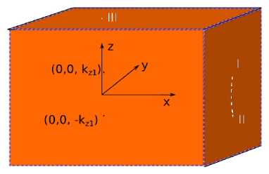
Figure 1: The figure shows projections of the two Weyl points on the $x-y$ (top) and $y-z$ (side) surfaces.

We will now study what happens if the top surface is illuminated by circularly polarized EMR with frequency $\omega$ and time period $T=2\pi/\omega$. In the case of circular polarization incident on the $x-y$ surface, the radiation produces the vector potential ${\vec{A}}(t)=A(\cos{\omega t},\eta\sin{\omega t},0)$ where $\eta=\pm 1$ for right and left circularly polarized beams, respectively. [Actually, since the radiation describes a wave traveling towards the $-{\hat{z}}$ direction, the arguments of $\cos$ and $\sin$ in ${\vec{A}}(t)$ should be $\omega t+kz$, where $k=\omega/c$. However, for the system parameters that we will consider below, $\omega z/c$ will be much smaller than 1. We will therefore ignore the term $kz=\omega z/c$.] We want to see if this periodic driving produces any states on the $x-y$ surface. To study this problem numerically, we introduce a one-dimensional (1D) lattice along the $\hat{z}$-direction and a continuum model along the $\hat{x}$ and $\hat{y}$ directions; hence $k_{x}$ and $k_{y}$ are good quantum numbers. We will use Floquet theory in order to compute the FEVs as a function of $(k_{x},k_{y})$, and we will then find the states which are localized near the $x-y$ surface using the inverse participation ratio as discussed below.

We introduce a lattice discretization of of the $z$ part of Eq. (1) as follows. We label the sites of the 1D lattice by integers $n$, with the total number of lattice points being equal to $N_{z}$; we will use open boundary conditions, with $n=1$ and $N_{z}$ denoting the top and bottom surfaces respectively. Each site will have two states corresponding to spin, $\sigma^{z}=\pm 1$; hence the wave function at each site $n$ will have two components, and the entire wave function will have $2N_{z}$ components. We will denote the lattice spacing by $a$ which we will take to be equal to 1 Å. We now define a lattice Hamiltonian which reduces to Eq. (1) in the limit $k_{z}a\to 0$. This can be done by replacing $k_{z}^{2}\to(2/a^{2})[1-\cos(k_{z}a)]=(1/a^{2})(2-e^{ik_{z}a}-e^{-ik_{z}a})$, and hence $k_{z}^{2}\psi_{n}\to(1/a^{2})(2\psi_{n}-\psi_{n+1}-\psi_{n-1})$ on the lattice. Equation (1) then takes the form

$$H\psi_{n} = [m_{0}~{}-~{}m_{2}(k_{x}^{2}+k_{y}^{2})]~{}\sigma^{z}~{}\psi_{n}$$ (4)

$$+~{}\frac{m_{1}}{a^{2}}~{}\sigma^{z}~{}[\psi_{n+1}~{}+~{}\psi_{n-1}~{}-~{}2\psi_{n}]$$

$$+~{}v~{}[\sigma^{x}k_{x}~{}+~{}\sigma^{y}k_{y}]~{}\psi_{n}.$$

We will set $a=1$ Å  henceforth.

Next, we include the vector potential of the circularly polarized EMR in the Hamiltonian. We assume that the amplitude of the vector potential has the form $A=A_{0}e^{-\gamma an}$, so that the amplitude of the vector potential decreases exponentially with a penetration length $1/\gamma$ as we move away from the $x-y$ surface and go into the bulk. It is realistic to assume this kind of exponential dependence as radiation usually gets absorbed in a medium. Adding the vector potentials to the momenta as $k_{x}\to k_{x}+A\cos\omega t$ and $k_{y}\to k_{y}+A\sin\omega t$, we see that Eq. (4) takes the form

$$H\psi_{n} = [m_{0}~{}-~{}m_{2}\{(k_{x}+A\cos{\omega t})^{2}$$ (5)

$$~{}~{}~{}~{}~{}~{}~{}~{}~{}~{}~{}~{}~{}~{}~{}+(k_{y}+A\sin{\omega t})^{2}\}]\sigma^{z}\psi_{n}$$

$$+v~{}[\sigma^{x}(k_{x}+A\cos{\omega t})+\sigma^{y}(k_{y}+A\sin{\omega t})]\psi_{n}$$

$$+~{}m_{1}\sigma^{z}[\psi_{n+1}+\psi_{n-1}-2\psi_{n}],$$

where we have assumed that the radiation is right circularly polarized ($\eta=1$).

We will numerically study the eigenvalues and eigenvectors of the Floquet operator $U$ which time evolves the system by one time period $T=2\pi/\omega$, namely,

$$U~{}=~{}{\cal T}e^{-i\int_{0}^{T}~{}dtH(t)},$$ (6)

where $\cal T$ denotes the time-ordered product. For a periodic Hamiltonian as in Eq. (5) which satisfies $H(t+T)=H(t)$, the Floquet operator has the property that its eigenvalues remain invariant if we shift the time by an arbitrary amount, i.e., $t\to t+\tau$. To see this, let us take $\tau$ to lie in the range $[0,T]$, and consider the Floquet operator corresponding to the time-shifted problem,

$$U^{\prime} = {\cal T}e^{-i\int_{\tau}^{T+\tau}~{}dtH(t)}$$ (7)

$$= {\cal T}e^{-i\int_{T}^{T+\tau}~{}dtH(t)}e^{-i\int_{\tau}^{T}~{}dtH(t)}$$

$$= {\cal T}e^{-i\int_{0}^{\tau}~{}dtH(t)}e^{-i\int_{\tau}^{T}~{}dtH(t)},$$

where we have used the fact that $H(t)$ is periodic in time with period $T$. If we define $U_{1}=e^{-i\int_{0}^{\tau}dtH(t)}$ and $U_{2}=e^{-i\int_{\tau}^{T}dtH(t)}$, we see that $U=U_{2}U_{1}$ while $U^{\prime}=U_{1}U_{2}$. Let $\chi$ be an eigenstate of $U$, with $U\chi=e^{i\theta}\chi$ (the eigenvalues of $U$ are unimodular since $U$ is unitary). This implies that

$$U_{2}U_{1}\chi = e^{i\theta}~{}\chi,$$

$$U_{1}U_{2}U_{1}\chi = e^{i\theta}~{}U_{1}\chi,$$

$$U^{\prime}(U_{1}\chi) = e^{i\theta}~{}(U_{1}\chi).$$ (8)

Hence, if $\chi$ is an eigenstate of $U$ with eigenvalue $e^{i\theta}$, then $U_{1}\chi$ is an eigenstate of $U^{\prime}$ with the same eigenvalue. Now, $U_{1}=e^{-i\int_{0}^{\tau}dtH(t)}$ gives the time evolution from $t=0$ to $t=\tau$. Thus if $\chi$ is the wave function at $t=0$, then $U_{1}\chi$ is the time evolved wave function at time $t=\tau$.

We will now use the above facts to show that although Eq. (5) contains two momenta $k_{x}$ and $k_{y}$, the eigenvalues of the Floquet operator $U$ only depends on the magnitude $k=\sqrt{k_{x}^{2}+k_{y}^{2}}$. To show this, let us assume that $k_{x}=k\cos\phi$ and $k_{y}=k\sin\phi$, and carry out a rotation by angle $\phi$ around the $z$-axis in the spin space,

$$\sigma^{\prime x} = \sigma^{x}\cos\phi+\sigma^{y}\sin\phi,$$

$$\sigma^{\prime y} = \sigma^{y}\cos\phi-\sigma^{x}\sin\phi.$$ (9)

We now look at the various terms in Eq. (5). The terms which are linear in $(k_{x},k_{y})$ and $(\sigma^{x},\sigma^{y})$ are given by

$$\sigma^{x}k_{x}+\sigma^{y}k_{y} = ~{}(\sigma^{\prime x}\cos\phi-\sigma^{\prime y}\sin\phi)~{}k\cos\phi$$

$$+~{}(\sigma^{\prime x}\sin\phi+\sigma^{\prime y}\cos\phi)~{}k\sin\phi$$

$$= \sigma^{\prime x}k,$$

$$k_{x}\cos\omega t+k_{y}\sin\omega t = k\cos(\omega t-\phi),$$

$$\sigma^{x}\cos\omega t+\sigma^{y}\sin\omega t = \sigma^{\prime x}\cos(\omega t-\phi)+\sigma^{\prime y}\sin(\omega t-\phi).$$

Hence Eq. (5) takes the form

$$H\psi_{n} = [m_{0}~{}-~{}m_{2}\{k^{2}+A^{2}$$ (11)

$$~{}~{}~{}~{}~{}~{}+2kA\cos(\omega t-\phi)\}]\sigma^{z}\psi_{n}$$

$$+v~{}[\sigma^{\prime x}\{k+A\cos(\omega t-\phi)\}$$

$$~{}~{}~{}~{}~{}+\sigma^{\prime y}A\sin(\omega t-\phi)]\psi_{n}$$

$$+~{}m_{1}\sigma^{z}[\psi_{n+1}+\psi_{n-1}-2\psi_{n}].$$

We can now use the arguments presented around Eqs. (7-8) to show that the eigenvalues of the Floquet operator of Eq. (11) do not depend on the value of $\phi$. It is therefore sufficient to set $\phi=0$ in Eq. (11) and study the FEVs as a function of $k$ alone. Namely, we can take $k_{x}=k$ and $k_{y}=0$ in Eq. (5).

Using the fact that the Pauli matrices $\sigma^{x}$ and $\sigma^{z}$ are real while $\sigma^{y}$ is imaginary, we can derive a symmetry of the Hamiltonian in Eq. (5) and therefore of $U$. We define a $2N_{z}$-dimensional matrix

$$\Sigma^{y}~{}=~{}I_{N_{z}}~{}\otimes~{}\sigma^{y},$$ (12)

where $I_{N_{z}}$ is the $N_{z}$-dimensional identity matrix. Namely, $\sigma^{y}$ has $N_{z}$ blocks along the diagonal, each block being equal to $\sigma^{y}$. We note that $(\Sigma^{y})^{2}=I_{2N_{z}}$. We then see that the Hamiltonian in Eq. (5) satisfies

$$\Sigma^{y}~{}H~{}\Sigma^{y}~{}=~{}-H^{*},$$ (13)

which implies that the Floquet operator in Eq. (6) satisfies

$$\Sigma^{y}~{}U~{}\Sigma^{y}~{}=~{}U^{*}.$$ (14)

This implies that if $U\psi_{1}=e^{i\theta}\psi_{1}$, then

$$\psi_{2}~{}=~{}\Sigma^{y}\psi_{1}^{*}$$ (15)

satisfies $U\psi_{2}=e^{-i\theta}\psi_{2}$.

III Numerical results

III.1 Surface states

In this section we present numerical results for the WSM under the effect of the periodic driving. We calculate the Floquet operator $U$ defined in Eq. (6) and find its eigenvectors $\psi_{j}$ and eigenvalues $e^{i\theta_{j}}$, where the $\theta_{j}$ lie in the range $[-\pi,\pi]$. [The Floquet eigenvalues are sometimes written as $e^{i\theta_{j}}=e^{-i\epsilon_{j}T}$, where $\epsilon_{j}$ are called the quasienergies; these lie in the range $[-\pi/T,\pi/T]$. However, we will generally work with the variable $\theta_{j}$ rather than $\epsilon_{j}$ due to the simplifying feature that the range of $\theta_{j}$ does not depend on $T$.] To identify the surface states, we calculate the inverse participation ratios (IPRs) of all the eigenvectors. The IPR for a state $\psi_{j}$ is defined as $I_{j}=\sum_{m=1}^{2N_{z}}|\psi_{j}(m)|^{4}$ (note that the states are normalized so that $\sum_{m=1}^{2N_{z}}|\psi_{j}(m)|^{2}=1$ for all $j$). States with large values of $I_{j}$ are more localized; we look at the wave functions of such states to find which of them are localized near the top surface ($n=1$).

The values of the parameters that we have used to find surface states are as follows gonzalez : $m_{0}=0.5$ eV, $m_{1}=0.605$ eV, $m_{2}=1$ eV Ų, $v=1$ eV Å, $k_{x}=k=0.5$ Å^-1, and $k_{y}=0$. In Fig. 2, we show the probabilities $|\psi_{j}(m)|^{2}$ versus $m$ for one of the surface states, taking $A_{0}=0.5$ Å^-1, $\gamma=0.0005$ Å^-1, $\omega=2$ eV$/\hbar$, and $N_{z}=200$ sites (hence the Hamiltonian is a $400$-dimensional matrix). Since $A=A_{0}e^{-\gamma an}$ (where $a=1$ Å  is the lattice spacing), the penetration length of the radiation is $1/\gamma=2000$ Å  which is much larger than the system size of $N_{z}a=200$ Å; this means the radiation decreases very little as we move away from the $x-y$ surface into the bulk. In Fig. 3, we show the probabilities of a surface state for $A_{0}=0.05$ and $N_{z}=400$ sites; all other parameters are the same as in Fig. 2. We find that the surface state has a bigger width. We will see later that the width of the surface state scales as an inverse power of the radiation amplitude $A_{0}$. (We find that it is necessary to give $\gamma$ a small but nonzero value to obtain surface states. If we set $\gamma=0$ exactly, we do not find any states localized near the surface).

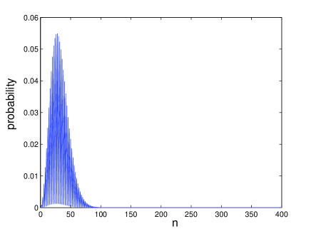
Figure 2: Probabilities vs $n$ for a surface state wave function for a system with $m_{0}=0.5$ eV, $m_{1}=0.605$ eV, $m_{2}=1$ eV Ų, $v=1$ eV Å, $k=0.5$ Å^-1, $A_{0}=0.5$ Å^-1, $\gamma=0.0005$ Å^-1, $\omega=2$ eV$/\hbar$, and 200 sites. The FEV of this state is $0.0363+0.9993i$.

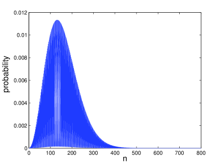
Figure 3: Probabilities vs $n$ for a surface state wave function for $A_{0}=0.05$ Å^-1, and 400 sites; all other parameters have the same values as in Fig. 2. The FEV of this state is $0.7521+0.6590i$.

Looking at the wave functions of the surface states, we find that two surface states $\psi_{1}$ and $\psi_{2}$ whose FEVs are complex conjugates of each other are related to each other as

$$\psi_{2}~{}=~{}\sigma^{y}\psi_{1}^{*},$$ (16)

as expected from Eq. (15).

We find numerically that states appear at the top surface for a range of momenta $k_{x}=k$ and $k_{y}=0$, where $k$ goes from, say, $k_{1}$ to $k_{2}$. This range depends on the various parameters of the model and the EMR. For example, for the parameters $m_{0},~{}m_{1},~{}m_{2},~{}v,~{}A_{0},~{}\gamma$ and $\omega$ used in Fig. 2, we find that there are at least two surface states (with complex conjugate FEVs) all the way from $k=0$ to $0.7$; hence $k_{1}=0$ and $k_{2}=0.7$. (For certain values of $k$, there are four or more surface states). Since the problem is rotationally invariant, this implies that there is an annular region of momentum $(k_{x},k_{y})$ given by $k_{1}<\sqrt{k_{x}^{2}+k_{y}^{2}}<k_{2}$ where there are two or more surface states. This region has a finite area given by $\pi(k_{2}^{2}-k_{1}^{2})$. Now consider a system whose top surface has a very large but finite area given by $\int dxdy=\cal A$. Then the total number of points in phase space, defined as $\int dk_{x}dk_{y}dxdy/(2\pi)^{2}$, where surface states appear is given by ${\cal A}(k_{2}^{2}-k_{1}^{2})/(4\pi)$. Hence the number of surface states is proportional to the surface area ${\cal A}$. Note however that the FEVs of these states depend on the value of $\sqrt{k_{x}^{2}+k_{y}^{2}}$; hence the degeneracy of the FEVs is not proportional to the area gonzalez .

It is interesting to study how the surface states evolve with time. Namely, given a surface state $\psi(0)$ which is an eigenstate of the Floquet operator in Eq. (6), we can study how

$$\psi(\tau)={\cal T}e^{-i\int_{0}^{\tau}~{}dtH(t)}~{}\psi(0)$$ (17)

changes with $\tau$ in the range $0\leq\tau\leq T$. [The arguments presented around Eqs. (7-8) show that $\psi(\tau)$ is the eigenstate of the time-shifted Floquet operator $U^{\prime}={\cal T}e^{-i\int_{\tau}^{T+\tau}dtH(t)}$ discussed in Eq. (7).] We have numerically studied how the wave function in Eq. (17) varies with $\tau$. We find that the variation is generally quite small. For instance, for the system parameters used in Fig. 3, the plots of probabilities versus $n$ for $\psi(0)$, $\psi(T/4)$, $\psi(T/2)$ and $\psi(3T/4)$ are found to be indistinguishable from each other on the scale of that figure.

We have examined if the surface states discussed in this section are stable to certain perturbations. We find that these states continue to exist when the perturbations are sufficiently small. For instance, we have studied the effect of a small random on-site potential (proportional to the $2\times 2$ identity matrix) added to the Hamiltonian in Eq. (5); the on-site potential $\epsilon(n)$ is taken from a uniform probability distribution in the range $[-\epsilon_{0},\epsilon_{0}]$, and is chosen independently at different sites $n$. (Such a term in the Hamiltonian breaks the symmetry described in Eq. (13), and hence the eigenvalues of the Floquet operator $U$ no longer come in complex conjugate pairs). Numerically we find that the surface states survive this perturbation, possibly with some changes in the shapes and peak positions of their wave functions, when $\epsilon_{0}\lesssim 0.1~{}vA_{0}$.

III.2 Bulk-boundary correspondence

We now consider the system with periodic boundary conditions in the $\hat{z}$-direction (namely, the site after $n=N_{z}$ is the same as the site at $n=1$). This gives us a bulk system which has no boundaries. We then look at the bulk states in the presence of radiation and see if there is any correspondence between the bulk states and the surface states that appear due to driving. In the previous section on surface states, we had taken the amplitude $A$ of the vector potential to decrease exponentially along the $\hat{z}$-direction as $A=A_{0}e^{-\gamma an}$. We took $\gamma$ to be very small, and the system size $N_{z}a$ to be much smaller than the penetration length $1/\gamma$ but much larger than the width of the surface states. As we will see later, the width of the surface states scales in such a way with $1/\gamma$ that the surface states survive in the limit $\gamma\to 0$ provided that we take the system size $N_{z}$ to be large enough. We will therefore set $\gamma=0$ in this section so that the radiation amplitude is uniform through out the system. Hence we have translational invariance along the $\hat{z}$-direction and the momentum $k_{z}$ is a good quantum number, along with $k_{x}$ and $k_{y}$. Setting $k_{x}=k$ and $k_{y}=0$ as before, the bulk Hamiltonian is found to be

$$H_{b} = [m_{0}~{}-~{}2m_{1}(1-\cos k_{z})$$

$$~{}-~{}m_{2}~{}(k^{2}~{}+~{}A_{0}^{2}~{}+~{}2kA_{0}\cos\omega t)]~{}\sigma^{z}$$

$$+~{}v~{}[\sigma^{x}(k+A_{0}\cos{\omega t})~{}+~{}\sigma^{y}A_{0}\sin\omega t].$$

This Hamiltonian is only a $2$-dimensional matrix unlike the Hamiltonian in the previous section which was $2N_{z}$-dimensional; hence the numerical calculations are much faster here. We find the eigenvalues of the Floquet operator $U={\cal T}e^{-i\int_{0}^{T}dtH_{b}(t)}$ as a function of $k_{z}$, for the values of the various parameters for which we got surface states in the previous section. [In analogy with the symmetry discussed in Eqs. (13-15), we find here that $\sigma^{y}H\sigma^{y}=-H^{*}$ which implies that $\sigma^{y}U\sigma^{y}=U^{*}$; hence the eigenvalues of $U$ are complex conjugates of each other for every value of $k_{z}$. It is also clear from Eq. (LABEL:ham5) that the eigenvalues of $U$ are the same for $k_{z}$ and $-k_{z}$.]

In Fig. 4 (a), we plot the real part, $\cos\theta$, of the FEVs ($e^{i\theta}$) as a function of $k_{z}$ for a bulk system with $m_{0}=0.5$ eV, $m_{1}=0.605$ eV, $m_{2}=1$ eV Ų, $v=1$ eV Å^-1, $k=0.5$ Å^-1, $A_{0}=0.05$ Å^-1, $\gamma=0$, $\omega=2$ eV$/\hbar$, and $N_{z}=800$ sites with periodic boundary conditions. We see that $\cos\theta$ has extrema at several values of $k_{z}$. Of these, the extrema at $\cos\theta=\pm 1$ are trivial in the sense that they arise simply because $\cos\theta$ lies in the range $[-1,1]$. The non-trivial extrema of $\cos\theta$ lie at $k_{z}=0.628$ and $2\pi-0.628$ where $\cos\theta=0.007$ and at $k_{z}=\pi$ where $\cos\theta=0.754$. As an alternative way of viewing these results, Fig. 4 (b) shows a plot of $\theta$ versus $k_{z}$ for the same system parameters. (For each value of $k_{z}$, there are two values of $\theta$ given by a $\pm$ pair). Once again we see some extrema lying at $k_{z}=0.628$ and $2\pi-0.628$ where $\theta=1.564$ and at $k_{z}=\pi$ where $\theta=0.721$.

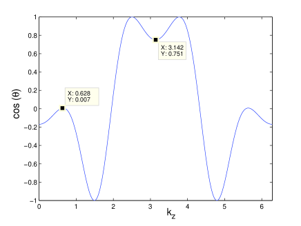
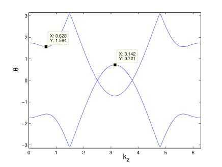
Figure 4: (a) Plot of $\cos(\theta)$ vs $k_{z}$ and (b) plot of $\theta$ vs $k_{z}$ for a bulk system with $m_{0}=0.5$ eV, $m_{1}=0.605$ eV, $m_{2}=1$ eV Ų, $v=1$ eV Å^-1, $k=0.5$ Å^-1, $A_{0}=0.05$ Å^-1, $\omega=2$ eV$/\hbar$, and 800 sites.

We now compare the extrema of $\theta$ for the bulk system with the values of $\theta$ for the surface states studied in the previous section for the 1D lattice system with the same parameter values (except that the previous section requires a small nonzero value of $\gamma=0.0005$ Å^-1). We find that the $\theta$ of the surface states match some of the extrema of $\theta$ of the bulk system. (For instance, the surface state shown in Fig. 3 has $\cos\theta=0.7521$ implying $\theta=0.720$; this is very close to the extremum value of $0.721$ that we see in Fig. 4 (b).) This is one kind of bulk-boundary correspondence.

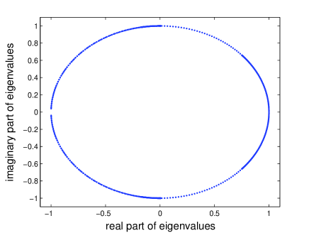
Figure 5: Plot of real and imaginary parts of the FEVs of the states of a bulk system with the same parameter values as in Fig. 4.

Figure 6: Density of states $\rho(\theta)$ as a function of $\theta$ in the range $[-\pi,\pi]$ for a bulk system with the same parameter values as in Fig. 4.

The fact that the FEVs of the bulk system have extrema as a function of $k_{z}$ can be visualized in a different way. Figure 5 shows the real and imaginary parts of the FEVs (these form a unit circle since the Floquet operator $U$ is unitary) for a system with the same parameters as in Fig. 4. We can see that the density of the eigenvalues is not uniform throughout the plot; it is denser in some parts compared to the other parts. Near any point $\theta^{\prime}$ where $\theta_{k_{z}}$ has an extremum, the density of states defined as

$$\rho(\theta)~{}=~{}\int_{0}^{2\pi}~{}\frac{dk_{z}}{2\pi}~{}\delta(\theta-\theta_{k_{z}})$$ (19)

will diverge for an infinitely large system and will have a sharp peak for a finite but large system. (In Eq. (19) we have normalized the density of states such that $\int_{-\pi}^{\pi}d\theta\rho(\theta)=1$). In Fig. 6 we show the density of states as a function of $\theta$. [In order to obtain a smooth curve, we have replaced the $\delta$-functions in Eq. (19) by Gaussians $\exp[-(\theta-\theta_{k_{z}})^{2}/\sigma^{2}]$, where $\sigma=0.0224$, and then summed over the $2N_{z}$ values of $\theta_{k_{z}}$.] We indeed see that the extrema in Fig. 4 (b) occurring at $\theta=0.721$ and $1.564$ agree well with some of the values of $\theta$ where the density of states has peaks as we have shown in Fig. 6. We can therefore restate the bulk-boundary correspondence by saying that the values of $\theta$ of the surface states match some of the points where the density of states has a peak in a plot like Fig. 6.

Next, we want to see if the values of $k_{z}$ where the $\theta$’s of the bulk system have extrema have any significance for the wave functions of the surface states. We know that the wave functions for the 1D lattice system with $N_{z}$ sites has $2N_{z}$ components due to the spin-1/2 degree of freedom. We therefore consider two different Fourier transforms of the wave function $\psi_{j}$ of a surface. These are defined as

$$f_{\uparrow}(k_{z}) = \frac{1}{N_{z}}\sum_{m=1,3,\cdots}e^{-ik_{z}m}~{}\psi_{j}(m),$$

$$f_{\downarrow}(k_{z}) = \frac{1}{N_{z}}\sum_{m=2,4,\cdots}e^{-ik_{z}m}~{}\psi_{j}(m),$$

for spin-up and spin-down electrons respectively.

In Fig. 7, we show plots of $|f_{\uparrow}(k_{z})|^{2}$ versus $k_{z}$ for two surface states with the parameter values as shown in Fig. 3; we have chosen surface states whose $\theta$’s match some of the extrema of the $\theta$’s of the bulk system as shown in Fig. 4 (b). We see that the peaks $|f_{\uparrow}(k_{z})|^{2}$ occur at the values of $k_{z}$ equal to $\pm 0.628$ and $3.142$; these are the same as the values of $k_{z}$ where the $\theta$’s of the bulk system shown in Fig. 4 (b) have extrema. (We obtain similar results if we plot $|f_{\downarrow}(k_{z})|^{2}$ versus $k_{z}$). This is another kind of bulk-boundary correspondence.

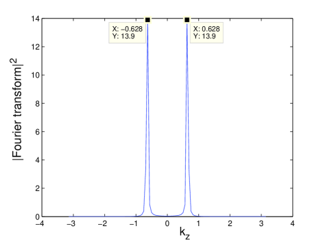
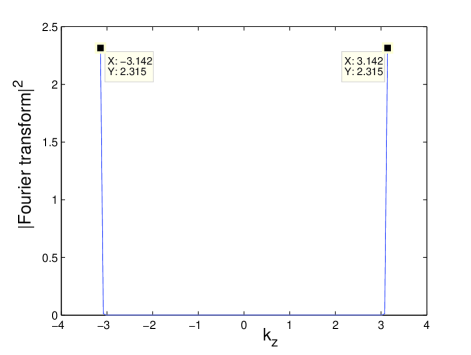
Figure 7: Plots of $|f_{\uparrow}(k_{z})|^{2}$ vs $k_{z}$ for two surface states whose $\theta$’s match some of the extrema of the $\theta$’s of the bulk states. The coordinates of the peaks of the Fourier transforms are shown in the figure. The system parameters are the same as in Fig. 3.

It would be useful to understand the reason for a correspondence between the extrema of the $\theta$’s of the bulk system and the $\theta$’s of the surface states. A possible reason may be as follows saha2 . We know that the presence of an extremum of the bulk $\theta$’s near a particular value, say, $\theta^{\prime}$ at $k_{z}=k^{\prime}$, means that the density of states $\rho(\theta)$ diverges as we approach $\theta=\theta^{\prime}$. The presence of a large number of bulk states near $(k^{\prime},\theta^{\prime})$ may make it easier for a system to superpose those states to form states which are localized at the surface. Such surface states will then naturally have a value of $\theta$ which lies close to $\theta^{\prime}$ and a Fourier transform whose peak is close to $k^{\prime}$.

Before ending this section, we would like to note that the values of $\theta$’s of the bulk and surface states are not separated by a gap. This raises the question, why are the surface states robust to certain kinds of perturbations, such as on-site disorder as discussed at the end of Sec. III.1?

III.3 Surface states at $k_{x}=k_{y}=0$

It turns out that the problem defined by Eq. (5) becomes much easier to solve and we can gain a much better understanding of the surface state wave functions for the special case $k_{x}=k_{y}=0$. We then get

$$H\psi_{n} = (m_{0}~{}-~{}2m_{1}~{}-~{}m_{2}A^{2})~{}\sigma^{z}~{}\psi_{n}$$ (20)

$$+~{}m_{1}~{}\sigma^{z}~{}(\psi_{n+1}~{}+~{}\psi_{n-1})$$

$$+~{}v~{}(\sigma^{x}A\cos{\omega t}~{}+~{}\sigma^{y}A\sin{\omega t})~{}\psi_{n},$$

where $A=A_{0}e^{-\gamma an}$. We will write $\psi_{n}=(a_{n},b_{n})^{T}$, where $a_{n}$ and $b_{n}$ denote the spin-up and spin-down components at the site $n$. The Schrödinger equation $i\partial\psi_{n}/\partial t=H\psi_{n}$ then takes the form

$$i\frac{\partial a_{n}}{\partial t} = (m_{0}~{}-~{}2m_{1}~{}-~{}A^{2})~{}a_{n}$$

$$+~{}m_{1}~{}(a_{n+1}~{}+~{}a_{n-1})~{}+~{}v~{}Ae^{-i\omega t}~{}b_{n},$$

$$i\frac{\partial b_{n}}{\partial t} = -~{}(m_{0}~{}-~{}2m_{1}~{}-~{}A^{2})~{}b_{n}$$

$$-~{}m_{1}~{}(b_{n+1}~{}+~{}b_{n-1})~{}+~{}v~{}Ae^{i\omega t}~{}a_{n}.$$

Interestingly, there is a transformation which makes Eqs. (LABEL:ab1) look time-independent. This is given by

$$a_{n}~{}=~{}{\tilde{\alpha}}_{n}~{}e^{-i\omega t/2}~{}~{}~{}~{}{\rm and}~{}~{}~{}~{}b_{n}~{}=~{}{\tilde{\beta}}_{n}~{}e^{i\omega t/2}.$$ (22)

Substituting this in Eq. (LABEL:ab1), we obtain

$$i\frac{\partial{\tilde{\alpha}}_{n}}{\partial t} = (m_{0}~{}-~{}2m_{1}~{}-~{}A^{2}~{}-~{}\frac{\omega}{2})~{}{\tilde{\alpha}}_{n}$$

$$+~{}m_{1}~{}({\tilde{\alpha}}_{n+1}~{}+~{}{\tilde{\alpha}}_{n-1})~{}+~{}vA~{}{\tilde{\beta}}_{n},$$

$$i\frac{\partial{\tilde{\beta}}_{n}}{\partial t} = -~{}(m_{0}~{}-~{}2m_{1}~{}-~{}A^{2}~{}-~{}\frac{\omega}{2})~{}{\tilde{\beta}}_{n}$$ (23)

$$-~{}m_{1}~{}({\tilde{\beta}}_{n+1}~{}+~{}{\tilde{\beta}}_{n-1})~{}+~{}vA~{}{\tilde{\alpha}}_{n}.$$

Next, we put ${\tilde{\alpha}}_{n}(t)=\alpha_{n}e^{-iEt}$ and ${\tilde{\beta}}_{n}(t)=\beta_{n}e^{-iEt}$ in the above equations. [This implies that $a_{n}(T)=-a_{n}(0)e^{-iET}$ and $b_{n}(T)=-b_{n}(0)e^{-iET}$, where we have used the fact that $e^{-i\omega T/2}=e^{-i\pi}=-1$. Hence the FEV is given by $e^{i\theta}=-e^{-iET}$.] We then find the completely time-independent equations

$$E\alpha_{n} = (m_{0}~{}-~{}2m_{1}~{}-~{}A^{2}~{}-~{}\frac{\omega}{2})~{}\alpha_{n}$$

$$+~{}m_{1}(\alpha_{n+1}~{}+~{}\alpha_{n-1})~{}+~{}vA~{}\beta_{n}$$

$$E\beta_{n} = -~{}(m_{0}~{}-~{}2m_{1}~{}-~{}A^{2}~{}-~{}\frac{\omega}{2})~{}\beta_{n}$$ (24)

$$-~{}m_{1}(\beta_{n+1}~{}+~{}\beta_{n-1})~{}+~{}vA~{}\alpha_{n}.$$

We have numerically solved Eqs. (24) for a finite system in which $n$ goes from 1 to $N_{z}$. We find several surface states $\psi_{j}$ which are localized near $n=1$ as in Figs. 2-3. For all these states, we find that the Fourier transform of both the components $a_{n}$ and $b_{n}$ are peaked at $k_{z}=\pi$. This means that $\alpha_{n}e^{i\pi n}=\alpha_{n}(-1)^{n}$ varies slowly on the scale of a lattice spacing (given by $a=1$ Å), and similarly for $\beta_{n}(-1)^{n}$. We therefore define the slowly varying quantities

$$\alpha^{\prime}_{n}~{}=~{}(-1)^{n}\alpha_{n}~{}~{}~{}~{}{\rm and}~{}~{}~{}~{}\beta^{\prime}_{n}~{}=~{}(-1)^{n}\beta_{n}.$$ (25)

Eqs. (24) then take the form

$$E\alpha^{\prime}_{n} = (m_{0}~{}-~{}2m_{1}~{}-~{}A^{2}~{}-~{}\frac{\omega}{2})~{}\alpha^{\prime}_{n}$$

$$-~{}m_{1}(\alpha^{\prime}_{n+1}~{}+~{}\alpha^{\prime}_{n-1})~{}+~{}vA~{}\beta^{\prime}_{n}$$

$$E\beta^{\prime}_{n} = -~{}(m_{0}~{}-~{}2m_{1}~{}-~{}A^{2}~{}-~{}\frac{\omega}{2})~{}\beta^{\prime}_{n}$$ (26)

$$+~{}m_{1}(\beta^{\prime}_{n+1}~{}+~{}\beta^{\prime}_{n-1})~{}+~{}vA~{}\alpha^{\prime}_{n}.$$

Since $\alpha^{\prime}_{n},~{}\beta^{\prime}_{n}$ are slowly varying, we can use the Taylor expansions $\alpha^{\prime}_{n+1}+\alpha^{\prime}_{n-1}=2\alpha^{\prime}_{n}+\partial^{2}\alpha^{\prime}_{n}/\partial z^{2}$ and $\beta^{\prime}_{n+1}+\beta^{\prime}_{n-1}=2\beta^{\prime}_{n}+\partial^{2}\beta^{\prime}_{n}/\partial z^{2}$, where $z=-na$ is now a continuous variable. [We have taken $z=-na$ because $n$ increases from zero while $z$ decreases from zero as we go down from the top surface; see Fig. 1. Hence $A=A_{0}e^{-\gamma an}=A_{0}e^{\gamma z}$.] We will henceforth write $\alpha^{\prime}_{n}=\alpha^{\prime}(z)$ and $\beta^{\prime}_{n}=\beta^{\prime}(z)$. Using this in Eqs. (26) gives

$$E\alpha^{\prime} = (m_{0}~{}-~{}4m_{1}~{}-~{}A^{2}~{}-~{}\frac{\omega}{2})~{}\alpha^{\prime}$$ (27)

$$-~{}m_{1}~{}\frac{\partial^{2}\alpha^{\prime}}{\partial z^{2}}~{}+~{}vA~{}\beta^{\prime},$$

$$E\beta^{\prime} = -~{}(m_{0}~{}-~{}4m_{1}~{}-~{}A^{2}~{}-~{}\frac{\omega}{2})~{}\beta^{\prime}$$ (28)

$$+~{}m_{1}~{}\frac{\partial^{2}\beta^{\prime}}{\partial z^{2}}~{}+~{}vA~{}\alpha^{\prime}.$$

Next, we find numerically that for the surface states, $E\simeq m_{0}-4m_{1}-\omega/2$, so that

$$\Delta E~{}=~{}E-(m_{0}-4m_{1}-\omega/2)~{}\ll~{}E.$$ (29)

We also find that $\beta^{\prime}$ is much smaller than $\alpha^{\prime}$ for the surface states; hence we can neglect the second order differential term in Eq. (28). We can also ignore the term $A^{2}=A_{0}^{2}e^{2\gamma z}$ in Eq. (28) if $A_{0}$ is small. That equation then gives $E\beta^{\prime}\simeq-E\beta^{\prime}+vA\alpha^{\prime}$ which implies

$$\beta^{\prime}~{}=~{}\frac{vA\alpha^{\prime}}{2E}.$$ (30)

Using Eqs. (29-30) in Eq. (27), we get

$$-~{}m_{1}~{}\frac{\partial^{2}\alpha^{\prime}}{\partial z^{2}}~{}+~{}\frac{v^{2}A^{2}}{2E}~{}\alpha^{\prime}~{}-~{}A^{2}\alpha^{\prime}~{}=~{}\Delta E~{}\alpha^{\prime}.$$ (31)

We now use the form $A=A_{0}e^{\gamma z}$. Further, since $\gamma$ is small and we are only interested in the region close to $z=0$ (the top surface), we can write $A=A_{0}(1+\gamma z)$. Putting all this together, we obtain

$$-\frac{\partial^{2}\alpha^{\prime}}{\partial z^{2}}~{}-~{}\frac{A_{0}^{2}}{m_{1}}~{}(1-\frac{v^{2}}{2E})~{}(1+2\gamma z)~{}\alpha^{\prime}~{}=~{}\frac{\Delta E}{m_{1}}~{}\alpha^{\prime}.$$ (32)

For the parameter values that we are using, $E\simeq m_{0}-4m_{1}-\omega/2$ is negative. Hence the quantity

$$C~{}=~{}\frac{2}{m_{1}}~{}(1-\frac{v^{2}}{2E})$$ (33)

is positive. Defining

$$D~{}=~{}\frac{\Delta E}{m_{1}}~{}+~{}\frac{A_{0}^{2}}{m_{1}}~{}(1-\frac{v^{2}}{2E}),$$ (34)

Eq. (32) takes the form

$$-\frac{\partial^{2}\alpha^{\prime}}{\partial z^{2}}~{}-~{}C\gamma A_{0}^{2}z\alpha^{\prime}~{}=~{}D\alpha^{\prime}.$$ (35)

This is the Schrödinger equation of a particle in a potential which increases linearly as $z$ decreases from zero, and there is a hard wall at $z=0$ since the particle cannot be in the region $z>0$ (which lies outside system).

We now define a rescaled variable

$$w~{}=~{}(C\gamma A_{0}^{2})^{1/3}~{}\left(z~{}+~{}\frac{D}{C\gamma A_{0}^{2}}\right).$$ (36)

Eq. (35) then takes the form

$$-\frac{\partial^{2}\alpha^{\prime}}{\partial w^{2}}~{}-~{}w\alpha^{\prime}_{n}~{}=~{}0.$$ (37)

This is known as the Airy equation; its solutions are given by the first and second kind of Airy functions denoted by $Ai(-w)$ and $Bi(-w)$ respectively. We want a solution of Eq. (37) which goes to zero as $w\to-\infty$; such a solution is given by $Ai(-w)$ which has the asymptotic form $Ai(-w)\sim\exp[-(2/3)(-w)^{3/2}]$ as $w\to-\infty$. In general a linearly increasing potential gives several bound states. The spreads of the wave functions of these bound states will be given by $\Delta w$ of order 1, which implies

$$\Delta z~{}\sim~{}\frac{1}{\gamma^{1/3}~{}A_{0}^{2/3}},$$ (38)

due to the form in Eq. (36).

We thus conclude that for a fixed amplitude of the radiation, $A_{0}$, the spread of the bound states is of order $a^{2/3}/\gamma^{1/3}$ (we have introduced the factor of $a^{2/3}$ for dimensional reasons), while the penetration length of the radiation is $1/\gamma$. Clearly, $1/\gamma$ is much larger than $a^{2/3}/\gamma^{1/3}$ if $1/(a\gamma)\gg 1$. It is therefore possible to choose $\gamma$ and the system size $N_{z}a$ in such a way that the spreads of the bound states are much smaller than $N_{z}a$ which, in turn, is much smaller than $1/\gamma$. This is the regime in which all our numerical calculations have been done. Note that since we have taken $N_{z}a\ll 1/\gamma$ for the system with surfaces in Sec. III.1, we are justified in doing the calculations for the bulk system in Sec. III.2 with $\gamma$ set equal to 0; this is necessary since we want the bulk system (with periodic boundary conditions) to be translation invariant in the $\hat{z}$-direction.

Eq. (38) implies that if $\gamma$ is held fixed and the radiation amplitude $A_{0}\to 0$, the spreads of the bound states diverge. This makes sense since we do not expect to find any bound states when $A_{0}=0$.

Fig. 8 shows four surface states with 0, 1, 2 and 3 nodes respectively, for a system with $m_{0}=0.5$ eV, $m_{1}=0.605$ eV, $m_{2}=1$ eV Ų, $v=1$ eV Å, $k_{x}=k_{y}=0$, $A_{0}=0.5$ Å^-1, $\gamma=0.0005$ Å^-1, $\omega=2$ eV$/\hbar$, and 200 sites.

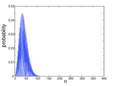
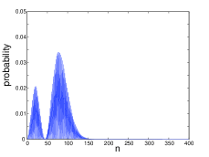
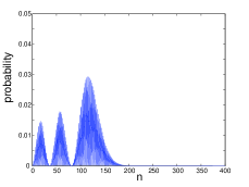
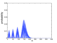
Figure 8: Probabilities vs $n$ for four surface state wave functions for a system with $m_{0}=0.5$ eV, $m_{1}=0.605$ eV, $m_{2}=1$ eV Ų, $v=1$ eV Å, $k_{x}=k_{y}=0$, $A_{0}=0.5$ Å^-1, $\gamma=0.0005$ Å^-1, $\omega=2$ eV$/\hbar$, and 200 sites.

Finally, we note that although we have derived the scaling relation in Eq. (38) for the case $k_{x}=k_{y}=0$, we expect this relation to hold even for other momenta as long as the amplitude $A_{0}$ of the EMR is small. A comparison of Figs. 2 and 3, where $k=0.5$ Å^-1, shows that the spread of the bound state indeed increases when $A_{0}$ decreases.

IV Effects of periodic driving on topological insulators

IV.1 Hamiltonian

We now study what happens when EMR applied to the top surface of a TI like $Bi_{2}Se_{3}$ wang3 . We begin with a bulk Hamiltonian for $Bi_{2}Se_{3}$ of the form qi

$$H = (-m+B_{1}k_{z}^{2})\tau^{z}~{}+~{}v_{z}k_{z}\tau^{y}$$ (39)

$$+~{}v_{\parallel}\tau^{x}(\sigma^{x}k_{y}-\sigma^{y}k_{x}),$$

where $m=0.28$ eV, $B_{1}=6.86$ eV Ų, $v_{z}=2.26$ eV Å, and $v_{\parallel}=3.33$ eV Å. Here the $\sigma^{i}$’s are Pauli spin matrices, and $\tau^{i}$’s denote Pauli pseudospin matrices with $\tau^{z}=\pm 1$ denoting $Bi$ and $Se$ respectively. In the presence of circularly polarized EMR applied to the top surface ($x-y$ surface located at $z=0$), the Hamiltonian becomes,

$$H = (-m+B_{1}k_{z}^{2})\tau^{z}+v_{z}k_{z}\tau^{y}$$

$$+v_{\parallel}\tau^{x}[\sigma^{x}(k_{y}+A\sin(\omega t))-\sigma^{y}(k_{x}+A\cos(\omega t))],$$

where we assume the form $A=A_{0}e^{\gamma z}$. As discussed in Sec. II, we again introduce a 1D lattice, with a lattice spacing $a=1$ Å, along the $\hat{z}$-direction. Each lattice point now has four components corresponding to spin $\sigma^{z}=\pm 1$ and pseudospin $\tau^{z}=\pm 1$ deb . To go from the continuum Hamiltonian in Eq. (LABEL:ham7) to a lattice Hamiltonian, we replace $k_{z}^{2}\to(2/a^{2})[1-\cos(k_{z}a)]=(2/a^{2})(1-(e^{ik_{z}a}+e^{-ik_{z}a})/2)$, and $k_{z}\to(1/a)[\sin(k_{z}a)]=(-i/a)[e^{ik_{z}a}+e^{-ik_{z}a}]$, assuming that $k_{z}a\ll 1$. We then set $a=1$ Å  as before. Following these substitutions, we obtain the action of the lattice Hamiltonian on the four-component wave function $\psi_{n}$

$$H\psi_{n} = -~{}m\tau^{z}\psi_{n}~{}+~{}2B_{1}\tau^{z}\psi_{n}~{}-~{}B_{1}\tau^{z}(\psi_{n+1}+\psi_{n-1})$$ (41)

$$-~{}\frac{i}{2}~{}v_{z}\tau^{y}(\psi_{n+1}-\psi_{n-1})$$

$$+~{}v_{\parallel}\tau^{x}[\sigma^{x}(k_{y}~{}+~{}A\sin(\omega t))$$

$$~{}~{}~{}~{}~{}~{}~{}~{}~{}~{}-~{}\sigma^{y}(k_{x}~{}+~{}A\cos(\omega t))]\psi_{n},$$

where $A=A_{0}e^{-\gamma n}$. As we discussed for the WSM, this Hamiltonian is again rotationally invariant; hence we can set $k_{y}=0$ henceforth.

IV.2 Numerical Results

We now numerically compute the Floquet operator

$$U~{}=~{}{\cal T}e^{-i\int_{0}^{T}dtH(t)},$$ (42)

where $T=2\pi/\omega$, and find its eigenvalues and eigenstates. We choose $k_{x}=k=0.5$ Å^-1 and $k_{y}=0$, and take the parameters of the EMR to be $A_{0}=1$ Å^-1, $\gamma=0.001$ Å^-1, $\omega=2$ eV$/\hbar$, and $N_{z}=200$ sites ($H$ and $U$ are therefore 800-dimensional matrices). We know that the $x-y$ surface of a TI hosts surface states even in the absence of any periodic driving. We therefore want to see whether the EMR generates any new surface states.

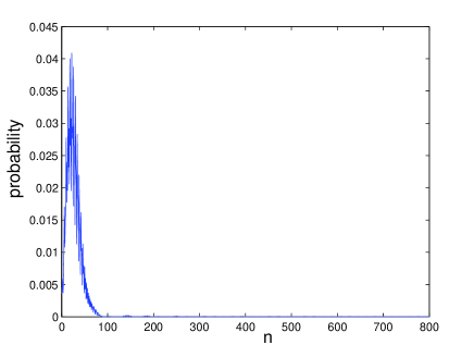
Figure 9: Probabilities vs $n$ for a state on the $x-y$ surface of a TI with a small decay length. The system parameters are $m=0.28$ eV, $B_{1}=6.86$ eV Ų, $v_{z}=2.26$ eV Å, $v_{\parallel}=3.33$ eV Å, $A_{0}=1$ Å^-1, $\gamma=0.001$ Å^-1, $\omega=2$ eV$/\hbar$, and 200 sites.

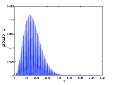
Figure 10: Probabilities vs $n$ for a state on the $x-y$ surface of a TI with a decay length which is much larger than the one in Fig. 9. The system parameters are the same as in Fig. 9.

We find that there are two types of surface states on the $x-y$ surface. There are some surface states which appear even in the absence of driving and have a decay length given by $v_{z}/m\sim 8$ Å; we call these the old surface states. Figure 9 shows this kind of a surface state. The decay lengths of these states are almost independent of the radiation amplitude. Figure 10 shows another kind of surface state which has a much larger decay length. These are the new states that appear due to periodic driving by the EMR. We find that the decay lengths of these states vary with the amplitude of the EMR just as we found for the surface states of a WSM in Sec. III.1.

If the value of the parameter $m$ in Eqs. (39-LABEL:ham7) is changed from $0.28$ eV to $-0.28$ eV, the system becomes a trivial insulator. When a circularly polarized EMR is applied to the $x-y$ surface of this system, we find numerically that the new kind of surface state with a large decay length again appears. However, the old states with a small  decay length does not appear; this is expected since a trivial insulator does not have any surface states in the absence of driving.

We have studied if a bulk-boundary correspondence exists for this system (either a TI or a trivial insulator) which has the same form as the correspondence that we found in Sec. III.2. We did not find such a correspondence here. This may be because this system is more complicated than a WSM in that the wave function has four components instead of two components at each site.

Just as in Sec. III.3, we find that it is much easier to study surface states in the special case where $k_{x}=k_{y}=0$. Once again, there is a unitary transformation which maps the Floquet problem to one in which we have to solve a time-independent problem. Namely, if we define

$$\psi_{n}~{}=~{}\exp[-\frac{i}{2}\omega t\sigma^{z}]{\tilde{\psi}}_{n},$$ (43)

followed by ${\tilde{\psi}}_{n}(t)={\tilde{\psi}}_{n}e^{-iEt}$, we obtain the equation

$$-m\tau^{z}{\tilde{\psi}}_{n}~{}+~{}2B_{1}\tau^{z}{\tilde{\psi}}_{n}-B_{1}\tau^{z}({\tilde{\psi}}_{n+1}+{\tilde{\psi}}_{n-1})$$

$$-~{}\frac{i}{2}~{}v_{z}\tau^{y}({\tilde{\psi}}_{n+1}-{\tilde{\psi}}_{n-1})~{}-~{}v_{\parallel}\tau^{x}\sigma^{y}A_{0}e^{-\gamma n}{\tilde{\psi}}_{n}$$

$$-~{}\frac{\omega}{2}\sigma^{z}{\tilde{\psi}}_{n}~{}=~{}E{\tilde{\psi}}_{n}.$$ (44)

This reproduces the solutions of the Floquet problem, with the Floquet eigenvalues being given by $e^{i\theta}=-e^{-iET}$. As before the surface states can be found by looking at the IPRs of all the solutions of Eq. (44) and identifying the ones with the largest IPRs.

V Conclusions

In this paper, we have studied the effects of EMR applied to the top surface of a WSM. We first introduced a simple model for a WSM which has only two Weyl points. The projections of these Weyl points on the different surfaces give the end points of Fermi arcs; these are curves lying in the Brillouin zones of those surfaces such that there are surface states whose momenta lie on the Fermi arcs. For the top surface of the WSM in our model, the Fermi arc is a single point; hence there is Fermi arc and no state on that surface in the time-independent system where the EMR is absent. We then studied the system in the presence of circularly polarized EMR applied to the top surface. We choose the case of circular polarization so that the Hamiltonian is invariant under rotations within the top surface.

To numerically look for surface states, we introduce a 1D lattice along the $\hat{z}$-direction. At each lattice point, denoted by an integer $n$, there are two states corresponding to the electron spin, $\sigma^{z}=\pm 1$. We take the amplitude of the vector potential of the EMR to be of the form $A=A_{0}e^{-\gamma an}$, where $1/\gamma$ is the penetration length of the radiation. It is realistic to assume this kind of exponential decay as radiation usually gets absorbed in a medium; we also find that this assumption is necessary for our calculations as surface states do not appear if we take an infinitely large penetration length. Due to the translational invariance of the surface, the momentum on the surface, $(k_{x},k_{y})$, is a good quantum number. We numerically calculate the Floquet operator $U$ which evolves the system through one time period $T=2\pi/\omega$, where $\omega$ is the frequency of the EMR. Using the rotational symmetry, we have shown that the FEVs do not depend on $k_{x}$ and $k_{y}$ separately, but only on the magnitude $k=\sqrt{k_{x}^{2}+k_{y}^{2}}$. Hence we have assumed $k_{x}=k$ and $k_{y}=0$ in all our calculations.

Given all the eigenstates of $U$, we find which of them describe surface states by calculating the IPRs of all the states and identifying the ones with large values of IPR. The surface states decay rapidly as we go into the bulk. Looking at the surface states for different values of the amplitude $A_{0}$ (specifically, $A_{0}=0.05$ and $0.5$), we find that the decay length of the surface state is larger if $A_{0}$ is smaller. We show later that there is a power law which relates the two quantities. We find that the number of surface states is proportional to the area of the surface.

For time-independent systems, it is known that a non-trivial bulk topology gives rise to states at the surfaces of the system. Hence there is a correspondence between the bulk bands and the surface states. We look for such a bulk-boundary correspondence in our system. To do this, we consider a bulk system with periodic boundary conditions along the $\hat{z}$-direction so that all the three momenta, $k_{x}$, $k_{y}$ and $k_{z}$, are good quantum numbers. We then plot $\theta$ (corresponding to the FEVs $e^{i\theta}$) of the bulk system as a function of $k_{z}$, for a given value of $k_{x}=k$ and $k_{y}=0$. We find that the values of $\theta$ of the surface states match some of the extrema of the $\theta$’s of the bulk states. To put this differently, the density of states $\rho(\theta)$ of the bulk system has peaks at certain values of $\theta$, and we find that some of these points match the $\theta$’s of the surface states. Next, we find the Fourier transform $f(k_{z})$ of the surface states as a function of $k_{z}$, for one particular spin component. We find that the peaks of $|f(k_{z})|^{2}$ occur at the same values of $k_{z}$ where the $\theta$’s of the bulk system have extrema. We therefore find two kinds of bulk-boundary correspondence, one between the values of $\theta$’s of the bulk and surface states and the other between the corresponding values of $k_{z}$.

We then study a special case of this problem where $k_{x}=k_{y}=0$. We find that this problem can be made completely time-independent by a unitary transformation. It is possible to solve the problem analytically in the continuum limit; we obtain a differential equation of the Airy form which explains why the numerically obtained surface state wave functions look like Airy functions. We find that the spread of these bound states scales with the amplitude $A_{0}$ and the penetration length $1/\gamma$ of the EMR as $1/(\gamma^{1/3}A_{0}^{2/3})$. Thus the spread of the bound states diverges if either $\gamma$ or $A_{0}$ goes to zero.

Finally, we study the effect of circularly polarized EMR on a TI. A TI has non-trivial topology in the bulk and hence hosts states at the surfaces even in the absence of EMR. We looked at the effects of the EMR to see if this generates a new kind of surface states. A numerical study of the Floquet operator $U$ shows that there are two kinds of surface states; one is the usual (old) surface state found in the time-independent system while the other is a new surface state whose decay length is much larger than that of the old surface state. The decay lengths of the new surface states can be tuned by varying the parameters of the EMR. We then find that if we consider a trivial insulator, there is no surface state in the absence of the EMR as expected; however, the application of EMR generates surface states which are similar to the new surface states generated in a TI. In analogy with the WSM, we have looked for a bulk-boundary correspondence for periodic driving of a TI, but have not found such a correspondence so far.

Turning to experimental methods for detecting the surface states generated by EMR, it may be possible to look for such states using time-resolved and angle-resolved photoemission spectroscopy wang3 and anomalous Hall conductivity chan . One can also try to measure the oscillating surface currents which are carried by the surface states gonzalez .

We will end by pointing out some directions for future studies. In this paper, we have only considered circularly polarized EMR; this simplifies the calculations due to rotational invariance. We can study what happens if the EMR is linearly polarized; in this case, the form of the surface states will depend on both $k_{x}$ and $k_{y}$, not just $\sqrt{k_{x}^{2}+k_{y}^{2}}$. It would be interesting to find the complete range of parameters (such as the frequency $\omega$ of the EMR and the surface momentum $(k_{x},k_{y})$) in which surface states appear. The stability of the surface states may be worth studying in detail. References gonzalez, ; gonzalez2, have argued that there is a topological protection because the momenta of the surface states are given by exceptional points which have a branch point structure. However, it would be useful to see if any topological invariants appear in this problem; this may help to analytically find the values of $\omega$ where surface states appear or disappear saha2 ; kitagawa2 ; thakurathi . For the WSM, we have only studied the states on the top surface ($x-y$) because we know that there are no states there in the absence of EMR. It would be interesting to study what happens on the other surfaces where states are present even when there is no EMR gonzalez .

References

- (1)
- (2) X. Wan, A. M. Turner, A. Vishwanath, and S. Y. Savrasov, Phys. Rev. B 83, 205101 (2011).
- (3) A. A. Burkov and L. Balents, Phys. Rev. Lett. 107, 127205 (2011).
- (4) G. B. Halasz and L. Balents, Phys. Rev. B 85, 035103 (2012).
- (5) P. Hosur, Phys. Rev. B 86, 195102 (2012).
- (6) A. A. Zyuzin and A. A. Burkov, Phys. Rev. B 86, 115133 (2012).
- (7) A. A. Zyuzin, S. Wu, and A. A. Burkov, Phys. Rev. B 85, 165110 (2012).
- (8) D. T. Son and B. Z. Spivak, Phys. Rev. B 88, 104412 (2013).
- (9) T. Ojanen, Phys. Rev. B 87, 245112 (2013).
- (10) P. Hosur and X. Qi, Comptes Rendus Physique 14, 857 (2013).
- (11) A. M. Turner and A. Vishwanath, arXiv:1301.0330.
- (12) K. Landsteiner, Phys. Rev. B 89, 075124 (2014).
- (13) A. C. Potter, I. Kimchi, and A. Vishwanath, Nat. Commun. 5, 5161 (2014).
- (14) O. Vafek and A. Vishwanath, Annu. Rev. Condens. Matter Phys. 5, 83112 (2014).
- (15) A. A. Burkov, Phys. Rev. B 91, 245157 (2015).
- (16) S. Rao, arXiv:1603.02821v2.
- (17) S.-Y. Xu, I. Belopolski, N. Alidoust, M. Neupane, G. Bian, C. Zhang, R. Sankar, G. Chang, Z. Yuan, C.-C. Lee, S. M. Huang, H. Zheng, J. Ma, D. S. Sanchez, B. Wang, A. Bansil, F. Chou, P. P. Shibayev, H. Lin, S. Jia, and M. Z. Hasan, Science 349, 613 (2015).
- (18) S.-Y. Xu, N. Alidoust, I. Belopolski, Z. Yuan, G. Bian, T.-R. Chang, H. Zheng, V. N. Strocov, D. S. Sanchez, G. Chang, C. Zhang, D. Mou, Y. Wu, L. Huang, C.-C. Lee, S.-M. Huang, B. Wang, A. Bansil, H.-T. Jeng, T. Neupert, A. Kaminski, H. Lin, S. Jia, and M. Z. Hasan, Nat. Phys. 11, 748 (2015).
- (19) B. Q. Lv, H. M. Weng, B. B. Fu, X. P. Wang, H. Miao, J. Ma, P. Richard, X. C. Huang, L. X. Zhao, G. F. Chen, Z. Fang, X. Dai, T. Qian, and H. Ding, Phys. Rev. X 5, 031013 (2015).
- (20) B. Q. Lv, N. Xu, H. M. Weng, J. Z. Ma, P. Richard, X. C. Huang, L. X. Zhao, G. F. Chen, C. E. Matt, F. Bisti, V. N. Strocov, J. Mesot, Z. Fang, X. Dai, T. Qian, M. Shi, and H. Ding, Nat. Phys. 11, 724 (2015).
- (21) S. Jia, S.-Y. Xu, and M. Z. Hasan, Nat. Mater. 15, 1140 (2016).
- (22) J. Behrends, A. G. Grushin, T. Ojanen, and J. H. Bardarson, Phys. Rev. B 93, 075114 (2016).
- (23) H.B. Nielsen and M. Ninomiya, Phys. Lett. B 105, 219 (1981).
- (24) J.-I. Inoue and A. Tanaka, Phys. Rev. Lett. 105, 017401 (2010).
- (25) N. H. Lindner, G. Refael, and V. Galitski, Nat. Phys. 7, 490 (2011).
- (26) T. Kitagawa, T. Oka, A. Brataas, L. Fu, and E. Demler, Phys. Rev. B 84, 235108 (2011).
- (27) N. H. Lindner, D. L. Bergman, G. Refael, and V. Galitski, Phys. Rev. B 87, 235131 (2013).
- (28) J. Cayssol, B. Dóra, F. Simon, and R. Moessner, Phys. Status Solidi RRL 7, 101 (2013).
- (29) P. Delplace, A. Gomez-Leon, and G. Platero, Phys. Rev. B 88, 245422 (2013).
- (30) Y. T. Katan and D. Podolsky, Phys. Rev. Lett. 110, 016802 (2013).
- (31) G. Usaj, P. M. Perez-Piskunow, L. E. F. Foa Torres, and C. A. Balseiro, Phys. Rev. B 90, 115423 (2014).
- (32) R. Wang, B. Wang, R. Shen, L. Sheng and D. Y. Xing, EPL 105, 17004 (2014).
- (33) L. D’Alessio and M. Rigol, Nat. Commun. 6, 8336 (2015).
- (34) A. Narayan, Phys. Rev. B 91, 205445 (2015).
- (35) Z. Yan and Z. Wang, Phys. Rev. Lett. 117, 087402 (2016).
- (36) K. Saha, Phys. Rev. B 94, 081103(R) 2016.
- (37) H. Hübener, M. A. Sentef, U. de Giovannini, A. F. Kemper, and A. Rubio, Nat. Commun. 8, 13940 (2017).
- (38) X.-X. Zhang, T. T. Ong, and N. Nagaosa, Phys. Rev. B 94, 235137 (2016).
- (39) L. Bucciantini, S. Roy, S. Kitamura, and T. Oka, arXiv:1612.01541.
- (40) Y. H. Wang, H. Steinberg, P. J. Herrero, and N. Gedik, Science 342, 453 (2013).
- (41) C.-K. Chan, P. A. Lee, K. S. Burch, J. H. Han, and Y. Ran, Phys. Rev. Lett. 116, 026805 (2016).
- (42) M. Kolodrubetz, B. M. Fregoso, and J. E. Moore, Phys. Rev. B 94, 195124 (2016).
- (43) J. Gonzalez and R. A. Molina, Phys. Rev. Lett. 116, 156803 (2016).
- (44) S. Saha, S. N. Sivarajan, and D. Sen, arXiv:1610.05963v2.
- (45) X.-L. Qi and S.-C. Zhang, Rev. Mod. Phys. 83, 1057 (2011).
- (46) O. Deb, A. Soori, and D. Sen, J. Phys. Condens. Matter 26, 315009 (2014).
- (47) J. Gonzalez and R. A. Molina, arXiv:1702.02521v2.
- (48) T. Kitagawa, E. Berg, M. Rudner, and E. Demler, Phys. Rev. B 82, 235114 (2010).
- (49) M. Thakurathi, A. A. Patel, D. Sen, and A. Dutta, Phys. Rev. B 88, 155133 (2013).