Abstract

The Uzawa method is a method for solving constrained optimization problems, and is often used in computational contact mechanics. The simplicity of this method is an advantage, but its convergence is slow. This paper presents an accelerated variant of the Uzawa method. The proposed method can be viewed as application of an accelerated projected gradient method to the Lagrangian dual problem. Preliminary numerical experiments suggest that the convergence of the proposed method is much faster than the original Uzawa method.

Keywords

Fast first-order method, accelerated gradient scheme, contact mechanics, nonsmooth mechanics, Uzawa method, convex optimization.

1 Introduction

It has been recognized well that contact mechanics has close relation with optimization and variational inequalities [6, 27]. The static frictionless contact problem of a linear elastic body, also called Signorini’s problem, is one of the most fundamental problems in contact mechanics. This is a boundary value problem to find the equilibrium configuration of an elastic body, where some portion of the boundary of the body can possibly touch the surface of a rigid obstacle (or the surface of another elastic body). Positive distance between the elastic body and the obstacle surface (i.e., positive gap) implies zero contact pressure (i.e., zero reaction), while nonzero reaction implies zero gap. This disjunction nature can be described by using complementarity conditions. Moreover, the frictionless contact problem can be formulated as a continuous optimization problem under inequality constraints [27].

The Uzawa method is known as a classical method for solving constrained optimization problems [2, 5, 25]. Due to ease in implementation, the Uzawa method is often applied to contact problems [22, 18, 12, 10, 21, 26, 20, 19]. Major drawback of the Uzawa method is that its convergence is slow; it exhibits only linear convergence in general.

Recently, accelerated, or “optimal” [14, 15], first-order methods have received substantial attention, particularly for solving large-scale optimization problems; see, e.g., [3, 4, 16, 13]. Advantages of most of these methods include ease of implementation, cheap computation per each iteration, and fast local convergence. Application of an accelerated first-order method to computational mechanics can be found in [11]. In this paper, we apply the acceleration scheme in [3] to the Uzawa method.

The paper is organized as follows. Section 2 provides an overview of the necessary background of the frictionless contact problem and the Uzawa method. Section 3 presents an accelerated Uzawa method. Section 4 reports the results of preliminary numerical experiments. Some conclusions are drawn in section 5.

In our notation, ^⊤ denotes the transpose of a vector or a matrix. For two vectors $\boldsymbol{x}=(x_{i})\in\mathbb{R}^{n}$ and $\boldsymbol{y}=(y_{i})\in\mathbb{R}^{n}$, we define

$$\min\{\boldsymbol{x},\boldsymbol{y}\}=(\min\{x_{1},y_{1}\},\dots,\min\{x_{n},y_{n}\})^{\top}.$$

We use $\mathbb{R}_{-}^{n}$ to denote the nonpositive orthant, i.e., $\mathbb{R}_{-}^{n}=\{\boldsymbol{x}=(x_{i})\in\mathbb{R}^{n}\mid x_{i}\leq 0\ (i=1,\dots,n)\}$. For $\boldsymbol{y}\in\mathbb{R}^{n}$, we use $\Pi_{-}(\boldsymbol{y})$ to denote the projection of $\boldsymbol{y}$ on $\mathbb{R}_{-}^{n}$, i.e.,

$$\Pi_{-}(\boldsymbol{y})=\operatornamewithlimits{\mathrm{arg\,min}}\{\|\boldsymbol{x}-\boldsymbol{y}\|\mid\boldsymbol{x}\in\mathbb{R}_{-}^{n}\}=\min\{\boldsymbol{y},\boldsymbol{0}\}.$$

We use $\mathop{\mathrm{diag}}\nolimits(\boldsymbol{x})$ to denote a diagonal matrix, the vector of diagonal components of which is $\boldsymbol{x}$.

2 Fundamentals of frictionless contact and Uzawa method

We briefly introduce the frictionless contact problem of an elastic body; see, e.g., [27] and [6] for fundamentals of contact mechanics.

Consider an elastic body subjected to a static load and a rigid obstacle fixed in space. Since the body cannot penetrate the surface of the obstacle, the deformation of the body is constrained from one side by the obstacle surface. We also assume the absence of friction and adhesion between the body surface and the obstacle surface. The set of these conditions is called the frictionless unilateral contact.

Suppose that the conventional finite element procedure is adopted for discretization of the elastic body. Let $\boldsymbol{u}\in\mathbb{R}^{d}$ denote the nodal displacement vector, where $d$ is the number of degrees of freedom of displacements. We use $\pi(\boldsymbol{u})$ to denote the total potential energy caused by $\boldsymbol{u}$. At the (unknown) equilibrium state, the nodes on a portion of the body surface can possibly make contact with the obstacle surface. Such nodes are called the contact candidate nodes, and the number of them is denoted by $m$. We use $g_{i}(\boldsymbol{u})$ $(i=1,\dots,m)$ to denote the gap between the $i$th contact candidate node and the obstacle surface. The non-penetration conditions are then formulated as

$$g_{i}(\boldsymbol{u})\geq 0,\quad i=1,\dots,m.$$ (1)

The displacement vector at the equilibrium state minimizes the total potential energy under the constraints in (1). Namely, the frictionless contact problem is formulated as follows:

$$\mathop{\mathrm{Minimize}} \pi(\boldsymbol{u})$$ (2a)

$$\mathop{\mathrm{subject~{}to}} g_{i}(\boldsymbol{u})\geq 0,\quad i=1,\dots,m.$$ (2b)

The Uzawa method solving problem (2) is listed in Algorithm 1 [2, 5, 25, 1]. It is worth noting that step 3 of Algorithm 1 can be performed as the equilibrium analysis with a conventional finite element code. Also, step 4 is simple to implement. Due to such ease in implementation, the Uzawa method is widely used in computational contact mechanics.

Algorithm 1 Uzawa method

1:$\alpha>0$, $\boldsymbol{r}^{(0)}\in\mathbb{R}_{-}^{m}$

2:for $k=0,1,\dots$ do

3:      $\boldsymbol{u}^{(k)}$ solves $\displaystyle\nabla\pi(\boldsymbol{u})+\sum_{i=1}^{m}r^{(k)}_{i}\nabla g_{i}(\boldsymbol{u})=\boldsymbol{0}$

4:      $r_{i}^{(k+1)}:=\min\{0,r_{i}^{(k)}+\alpha g_{i}(\boldsymbol{u}^{(k)})\}$ $(i=1,\dots,m)$

5:end for

As shown in Ciarlet [5, section 9.4], the Uzawa method can be viewed as a projected gradient method solving the Lagrange dual problem. Essentials of this observation are repeated here. The Lagrangian $L:\mathbb{R}^{d}\times\mathbb{R}^{m}\to\mathbb{R}\cup\{-\infty\}$ associated with problem (2) is given by

$$L(\boldsymbol{u},\boldsymbol{r})=\begin{dcases*}\pi(\boldsymbol{u})+\sum_{i=1}^{m}r_{i}g_{i}(\boldsymbol{u})&if $\boldsymbol{r}\leq\boldsymbol{0}$,\\ -\infty&otherwise.\end{dcases*}$$ (3)

Here, the Lagrange multipliers, $r_{1},\dots,r_{m}$, correspond to the reactions. The inequality constraints imposed on the reactions in (3) correspond to the non-adhesion conditions. Define $\psi:\mathbb{R}^{m}\to\mathbb{R}\cup\{-\infty\}$ by

$$\psi(\boldsymbol{r})=\inf\{L(\boldsymbol{u},\boldsymbol{r})\mid\boldsymbol{u}\in\mathbb{R}^{d}\},$$ (4)

which is the Lagrange dual function. The Lagrange dual problem of (2) is then formulated as follows:

$$\mathop{\mathrm{Maximize}} \psi(\boldsymbol{r})$$ (5a)

$$\mathop{\mathrm{subject~{}to}} \boldsymbol{r}\leq\boldsymbol{0}.$$ (5b)

Since $\psi$ is the pointwise infimum of a family of affine functions of $\boldsymbol{r}$, it is concave (even if problem (2) is not convex). Therefore, the dual problem (5) is convex.

Let $\alpha>0$ be an arbitrary constant. A point $\boldsymbol{r}\in\mathbb{R}^{m}$ is optimal for problem (5) if and only if it satisfies

$$\boldsymbol{r}=\Pi_{-}(\boldsymbol{r}+\alpha\nabla\psi(\boldsymbol{r})).$$ (6)

This fixed point relation yields the iteration of the projected gradient method as follows (see, e.g., [17]):

$$\boldsymbol{r}^{(k+1)}:=\Pi_{-}(\boldsymbol{r}^{(k)}+\alpha\nabla\psi(\boldsymbol{r}^{(k)})).$$ (7)

Here, $\alpha$ plays a role of the step size. For given $\bar{\boldsymbol{r}}\in\mathbb{R}_{-}^{m}$, define $\boldsymbol{u}_{\bar{\boldsymbol{r}}}$ by

$$\boldsymbol{u}_{\bar{\boldsymbol{r}}}=\operatornamewithlimits{\mathrm{arg\,min}}\{L(\boldsymbol{u},\bar{\boldsymbol{r}})\mid\boldsymbol{u}\in\mathbb{R}^{d}\}.$$ (8)

It can be shown that the relations

$$\frac{\partial}{\partial r_{i}}\psi(\bar{\boldsymbol{r}})=g_{i}(\boldsymbol{u}_{\bar{\boldsymbol{r}}}),\quad i=1,\dots,m$$ (9)

holds, when $\pi$ is convex and $g_{1},\dots,g_{m}$ are concave [5, Theorem 9.3-3]. Substitution of (9) into (7) results in step 4 of Algorithm 1. Thus, the Uzawa method for problem (2) is viewed as the projected gradient method applied to the Lagrange dual problem (5). It is worth noting that a reasonable stopping criterion,

$$\|\boldsymbol{r}^{(k)}-\boldsymbol{r}^{(k+1)}\|\leq\epsilon$$

with threshold $\epsilon$, is derived from the optimality condition in (6).

If we assume the small deformation, the total potential energy is given by

$$\pi(\boldsymbol{u})=\frac{1}{2}\boldsymbol{u}^{\top}K\boldsymbol{u}-\boldsymbol{p}^{\top}\boldsymbol{u}.$$

Here, $K\in\mathbb{R}^{d\times d}$ is the stiffness matrix, which is a constant positive definite symmetric matrix, and $\boldsymbol{p}\in\mathbb{R}^{d}$ is the external nodal force vector. Moreover, $g_{i}$ is linearized as

$$g_{i}(\boldsymbol{u})=h_{i}-\boldsymbol{n}_{i}^{\top}\boldsymbol{u},\quad i=1,\dots,m.$$ (10)

For notational simplicity, we rewrite (10) as

$$\boldsymbol{g}(\boldsymbol{u})=\boldsymbol{h}-N\boldsymbol{u},$$

where $\boldsymbol{h}\in\mathbb{R}^{m}$ is a constant vector, and $N\in\mathbb{R}^{m\times d}$ is a constant matrix. The upshot is that, in the small deformation theory, the frictionless contact problem is reduced to the following convex quadratic programming (QP) problem:

$$\mathop{\mathrm{Minimize}} \frac{1}{2}\boldsymbol{u}^{\top}K\boldsymbol{u}-\boldsymbol{p}^{\top}\boldsymbol{u}$$ (11a)

$$\mathop{\mathrm{subject~{}to}} \boldsymbol{h}-N\boldsymbol{u}\geq\boldsymbol{0}.$$ (11b)

The step size, $\alpha$, of the Uzawa method for solving problem (11) is chosen as follows. Let $\lambda_{1}(K)$ and $\sigma_{d}(N)$ denote the minimum eigenvalue of $K$ and the maximum singular value of $\sigma_{d}(N)$. If $\alpha$ is chosen so that

$$\alpha\in]0,2\lambda_{1}(K)/\sigma_{d}(N)[,$$

then it is shown that the Uzawa method converges [5, section 9.4].

3 Accelerated Uzawa method

In this section, we present an accelerated version of the Uzawa method.

The Uzawa method in Algorithm 1 is essentially viewed as the projected gradient method (7). This method is considered a special case of the proximal gradient method, because the proximal operator of the indicator function of a nonempty closed convex set is reduced to the projection onto the set [17]. Therefore, it is natural to apply the acceleration scheme for the proximal gradient method [3] to the projected gradient update (7). This results in the update

$$\boldsymbol{r}^{(k+1)} :=\Pi_{-}(\boldsymbol{\rho}^{(k)}+\alpha\nabla\psi(\boldsymbol{\rho}^{(k)})),$$ (12)

$$\boldsymbol{\rho}^{(k+1)} :=\boldsymbol{r}^{(k)}+\omega_{k+1}(\boldsymbol{r}^{(k+1)}-\boldsymbol{r}^{(k)}).$$ (13)

Here, $\omega_{k}\in[0,1)$ is an extrapolation parameter which is to be determined so that the convergence acceleration is achieved. In [3], $\omega_{k}$ is chosen as

$$\tau_{k+1} :=\frac{1}{2}\Bigl{(}1+\sqrt{1+\tau_{k}^{2}}\Bigr{)},$$

$$\omega_{k+1} :=\frac{\tau_{k}-1}{\tau_{k+1}}$$

with $\tau_{0}:=1$. The sequence of the dual objective values, $\{\psi(\boldsymbol{r}^{(k)})\}$, converges to the optimal value with rate $O(1/k^{2})$ [3].

The accelerated method in (12) and (13) is not guaranteed to be monotone in the dual objective value. Therefore, we follow O’Donoghue and Candès [16] in incorporating an adaptive restart technique of the acceleration scheme. Namely, we perform the restart procedure whenever the momentum term, $\boldsymbol{r}^{(k+1)}-\boldsymbol{r}^{(k)}$, and the gradient of the objective function, $\nabla\psi(\boldsymbol{r}^{(k)})$, make an obtuse angle, i.e.,

$$\nabla\psi(\boldsymbol{r}^{(k)})^{\top}(\boldsymbol{r}^{(k+1)}-\boldsymbol{r}^{(k)})<0.$$

As the upshot, the accelerated Uzawa method with adaptive restart is listed in Algorithm 2. One reasonable stopping criterion is

$$\|\boldsymbol{\rho}^{(k)}-\boldsymbol{r}^{(k+1)}\|\leq\epsilon$$ (14)

at step 5.

Algorithm 2 accelerated Uzawa method with restart

1:$\alpha>0$, $\boldsymbol{r}^{(0)}\in\mathbb{R}_{-}^{m}$, $\boldsymbol{\rho}^{(0)}:=\boldsymbol{r}^{(0)}$, $\tau_{0}:=1$

2:for $k=0,1,\dots$ do

3:      $\boldsymbol{u}^{(k)}$ solves $\displaystyle\nabla\pi(\boldsymbol{u})+\sum_{i=1}^{m}\rho_{i}^{(k)}\nabla g_{i}(\boldsymbol{u})=\boldsymbol{0}$

4:      $\boldsymbol{\gamma}^{(k)}:=\boldsymbol{g}(\boldsymbol{u}^{(k)})$

5:      $\boldsymbol{r}^{(k+1)}:=\min\{\boldsymbol{0},\boldsymbol{\rho}^{(k)}+\alpha\boldsymbol{\gamma}^{(k)}\}$

6:     $\displaystyle\tau_{k+1}:=\frac{1}{2}\Bigl{(}1+\sqrt{1+4\tau_{k}^{2}}\Bigr{)}$

7:     if $(\boldsymbol{\gamma}^{(k)})^{\top}(\boldsymbol{r}^{(k+1)}-\boldsymbol{r}^{(k)})\geq 0$ then

8:         $\displaystyle\boldsymbol{\rho}^{(k+1)}:=\boldsymbol{r}^{(k+1)}+\frac{\tau_{k}-1}{\tau_{k+1}}(\boldsymbol{r}^{(k+1)}-\boldsymbol{r}^{(k)})$

9:     else

10:         $\boldsymbol{\rho}^{(k+1)}:=\boldsymbol{r}^{(k+1)}$

11:         $\tau_{k+1}:=1$

12:     end if

13:end for

In the case of the small deformation theory, steps 3 and 4 of Algorithm 2 are simplified as follows.

• Step 3: Let $\boldsymbol{u}^{(k)}$ be the solution to the system of linear equations

  $$K\boldsymbol{u}=\boldsymbol{p}+N^{\top}\boldsymbol{\rho}^{(k)}.$$ (15)

  Here, the coefficient matrix $K$ is common to all the iterations. Hence, we carry out the Cholesky factorization only at the first iteration; at the following iterations, we can solve (15) only with the back-substitutions.

• Step 4: $\boldsymbol{\gamma}^{(k)}:=\boldsymbol{h}-N\boldsymbol{u}^{(k)}$.

4 Preliminary numerical experiments

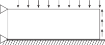
Figure 1: An elastic body on the obstacle.

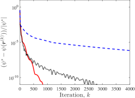
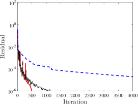
Figure 2: Convergence history for $(N_{X},N_{Y})=(30,10)$. 2 The dual objective value; and 2 the total residual. “Solid line” the accelerated Uzawa method with restart; “dotted line” the accelerated Uzawa method without restart; and “dashed line” the Uzawa method.

Consider an elastic body shown in Figure 1. The body is in the plane-stress state, with thickness $5\,\mathrm{mm}$, width $60\,\mathrm{mm}$, and height $20\,\mathrm{mm}$. It consists of an isotropic homogeneous material with Young’s modulus $200\,\mathrm{GPa}$ and Poisson’s ratio $0.3$. The bottom edge of the body is on the rigid obstacle, and the left edge is fixed by supports. The uniform downward traction of $50\,\mathrm{kPa}$ is applied to the top edge, and the uniform upward traction of $500\,\mathrm{kPa}$ is applied to the right edge. The body is discretized into $N_{X}\times N_{Y}$ four-node quadrilateral (Q4) finite elements, where $N_{X}$ $(=3N_{Y})$ is varied to generate problem instances with different sizes. The number of degrees of freedom of displacements is $d=2N_{X}(N_{Y}+1)$ and the number of contact candidate nodes is $m=N_{X}$. At the equilibrium state, about 73.3% of contact candidate nodes are in contact with nonzero reactions. We assume the small deformation, and solve QP problem (11). Computation was carried out on a $2.2\,\mathrm{GHz}$ Intel Core i5 processor with $8\,\mathrm{GB}$ RAM.

The proposed algorithm was implemented with MATLAB ver. 9.0.0. The threshold for the stopping criteria in (14) is set to $\epsilon=10^{-6}$. Comparison was performed with QUADPROG [23], SDPT3 ver. 4.0 [24] with CVX ver. 2.1 [9], and PATH ver. 4.7.03 [8] via the MATLAB Interface [7]. QUADPROG is a MATLAB built-in function for QP. We use an implementation of an interior-point method with setting the termination threshold, the parameter TolFun, to $10^{-8}$. SDPT3 implements a primal-dual interior-point method for solving conic programming problems. A QP problem is converted to the standard form of conic programming by CVX, where the parameter cvx_precision for controlling the solver precision is set to high. PATH is a nonsmooth Newton method to solve mixed complementarity problems, and hence can solve the KKT condition for QP.

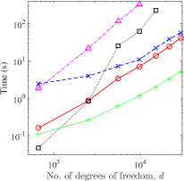
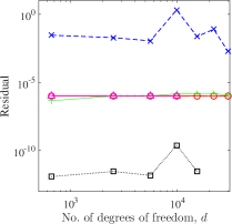
Figure 3: Comparison of 3 the computational time; and 3 the total residual. “$\circ$” The accelerated Uzawa method with restart; “$\triangle$” the Uzawa method; “$\times$” SDPT3; “$+$” QUADPROG; and “$\square$” PATH.

Figure 2 reports the convergence history of the proposed algorithm (Algorithm 2). It also shows the result of the accelerated Uzawa method without restart scheme, and that of Algorithm 1 (i.e., the Uzawa method without acceleration). Figure 2 shows the convergence history of the dual objective function. It is observed that the acceleration and restart schemes drastically speed up the convergence. Particularly, with the proposed algorithm, the dual objective value seems to converge quadratically and monotonically. The residual in Figure 2 is defined by using the KKT condition. Namely, we define vectors $\boldsymbol{e}_{j}$ $(j=1,2,3,4)$ by

$$\boldsymbol{e}_{1} =K\boldsymbol{u}^{(k)}-\boldsymbol{f}-N^{\top}\boldsymbol{r}^{(k)},$$

$$\boldsymbol{e}_{2} =\min\{\boldsymbol{g}(\boldsymbol{u}^{(k)}),\boldsymbol{0}\},$$

$$\boldsymbol{e}_{3} =\max\{\boldsymbol{r}^{(k)},\boldsymbol{0}\},$$

$$\boldsymbol{e}_{4} =-\mathop{\mathrm{diag}}\nolimits(\boldsymbol{g}(\boldsymbol{u}^{k}))\boldsymbol{r}^{(k)},$$

and the value of $\|(\boldsymbol{e}_{1},\boldsymbol{e}_{2},\boldsymbol{e}_{3},\boldsymbol{e}_{4})\|$ is reported in Figure 2.

Figure 3 compares the computational results of the five methods. It is observed in Figure 3 that QUADPROG is fastest for almost all the problem instances. The computational time required by PATH is very small for small instances, but drastically increases as the instance size increases. On the other hand, it is observed in Figure 3 that PATH converges to the highest accuracy. For large instances, the proposed method is the second-fastest method among the five methods. The computational time of SDPT3 is larger than that of the proposed method. Also, SDPT3 converges to the lowest accuracy. The residuals of the solutions obtained by the proposed method, the unaccelerated Uzawa method, and QUADPROG are similar. The computational time required by the unaccelerated Uzawa method is very large.

The upshot is that, within the small deformation theory, the proposed method is quite efficient, but the interior-point method for QP (QUADPROG) is more efficient. If we consider large deformation, problem (2) is not convex, and hence QUADPROG and SDPT3 cannot be adopted. Efficiency of the proposed method, that solves the convex dual problem, remains to be studied.

5 Concluding remarks

This paper has presented an accelerated Uzawa method. The method can be recognized as an accelerated projected gradient method solving the Lagrangian dual problem of a constrained optimization problem. It has been shown in the numerical experiments that the acceleration and restart schemes drastically speed up the convergence of the Uzawa method. Besides, the proposed method is easy to implement.

Many possibilities of extensions could be considered. To update the primal variables, the Uzawa method solves a system of linear equations. For large-scale problems, this process might be replaced by a fast first-order minimization method of a convex quadratic function, e.g., [13]. Also, an extension to large deformation problems remains to be explored.

Acknowledgments

This work is partially supported by JSPS KAKENHI 26420545 and 17K06633.

References

- Alart and Curnier [1991] P. Alart, A. Curnier: A mixed formulation for frictional contact problems prone to Newton like solution methods. Computer Methods in Applied Mechanics and Engineering, 92, 353–375 (1991).
- Allaire [2007] G. Allaire: Numerical Analysis and Optimization. Oxford University Press, New York (2007).
- Beck and Teboulle [2009] A. Beck, M. Teboulle: A fast iterative shrinkage-thresholding algorithm for linear inverse problems. SIAM Journal on Imaging Sciences, 2, 183–202 (2009).
- Becker et al. [2011] S. Becker, J. Bobin, E. J. Candès: NESTA: A fast and accurate first-order method for sparse recovery. SIAM Journal on Imaging Sciences, 4, 1–39 (2011).
- Ciarlet [1989] P. G. Ciarlet: Introduction to Numerical Linear Algebra and Optimisation. Cambridge University Press, Cambridge (1989).
- Duvaut and Lions [1976] G. Duvaut, J. L. Lions: Inequalities in Mechanics and Physics. Springer-Verlag, Berlin (1976).
- Ferris and Munson [1999] M. C. Ferris, T. S. Munson: Interfaces to PATH 3.0: Design, implementation and usage. Computational Optimization and Applications, 12, 207–227 (1999).
- Ferris and Munson [2000] M. C. Ferris, T. S. Munson: Complementarity problems in GAMS and the PATH solver. Journal of Economic Dynamics and Control, 24, 165–188 (2000).
- Grant and Boyd [2008] M. Grant, S. Boyd: Graph implementations for nonsmooth convex programs. In: V. Blondel, S. Boyd, H. Kimura (eds.), Recent Advances in Learning and Control (A Tribute to M. Vidyasagar), Springer (2008). pp. 95–110.
- Haslinger et al. [2004] J. Haslinger, R. Kučera, Z. Dostál: An algorithm for the numerical realization of 3D contact problems with Coulomb friction. Journal of Computational and Applied Mathematics, 164–165, 387–408 (2004).
- Kanno [2016] Y. Kanno: A fast first-order optimization approach to elastoplastic analysis of skeletal structures. Optimization and Engineering, 17, 861–896 (2016).
- Koko [2009] J. Koko: Uzawa block relaxation domain decomposition method for a two-body frictionless contact problem. Applied Mathematics Letters, 22, 1534–1538 (2009).
- Lee and Sidford [2013] Y. T. Lee, A. Sidford: Efficient accelerated coordinate descent methods and faster algorithms for solving linear systems. IEEE 54th Annual Symposium on Foundations of Computer Science, Berkeley (2013) pp. 147–156.
- Nesterov [1983] Y. Nesterov: A method of solving a convex programming problem with convergence rate . Soviet Mathematics Doklady, 27, 372–376 (1983).
- Nesterov [2004] Y. Nesterov: Introductory Lectures on Convex Optimization: A Basic Course. Kluwer Academic Publishers, Dordrecht (2004).
- O’Donoghue and Candès [2015] B. O’Donoghue, E. Candès: Adaptive restart for accelerated gradient schemes. Foundations of Computational Mathematics, 15, 715–732 (2015).
- Parikh and Boyd [2014] N. Parikh, S. Boyd: Proximal algorithms. Foundations and Trends in Optimization, 1, 127–239 (2014).
- Puso et al. [2008] M. A. Puso, T. A. Laursen, J. Solberg: A segment-to-segment mortar contact method for quadratic elements and large deformations. Computer Methods in Applied Mechanics and Engineering, 197, 555–566 (2008).
- Raous [1999] M. Raous: Quasistatic Signorini problem with Coulomb friction and coupling to adhesion. In: P. Wriggers, P. Panagiotopoulos (eds.), New Developments in Contact Problems, Springer-Verlag, Wien (1999) pp. 101–178.
- Rudoy [2015] E. M. Rudoy: Domain decomposition method for a model crack problem with a possible contact of crack edges. Computational Mathematics and Mathematical Physics, 55, 305–316 (2015).
- Temizer [2012] İ. Temizer: A mixed formulation of mortar-based frictionless contact. Computer Methods in Applied Mechanics and Engineering, 223–224, 173–185 (2012).
- Temizer et al. [2012] İ. Temizer, P. Wriggers, T. J. R. Hughes: Three-dimensional mortar-based frictional contact treatment in isogeometric analysis with NURBS. Computer Methods in Applied Mechanics and Engineering, 209–212, 115–128 (2012).
- The MathWorks, Inc. [2016] The MathWorks, Inc.: MATLAB Documentation. http://www.mathworks.com/ (Accessed November 2016).
- Tütüncü et al. [2003] R. H. Tütüncü, K. C. Toh, M. J. Todd: Solving semidefinite-quadratic-linear programs using SDPT3. Mathematical Programming, B95, 189–217 (2003).
- Uzawa [1958] H. Uzawa: Iterative methods for concave programming. In: K. J. Arrow, L. Hurwicz, H. Uzawa (eds.), Studies in Linear and Non-Linear Programming, Stanford University Press, Stanford (1958) pp. 154–165.
- Vikhtenko and Namm [2007] E. M. Vikhtenko, R. V. Namm: Duality scheme for solving the semicoercive Signorini problem with friction. Computational Mathematics and Mathematical Physics, 47, 1938–1951 (2007).
- Wriggers [2006] P. Wriggers: Computational Contact Mechacnics (2nd ed.). Springer-Verlag, Berlin (2006).
- Zavarise and De Lorenzis [2012] G. Zavarise, L. De Lorenzis: An augmented Lagrangian algorithm for contact mechanics based on linear regression. International Journal for Numerical Methods in Engineering, 91, 825–842 (2012).