The influence of measurement error on Maxwell’s demon

Abstract

In any general cycle of measurement, feedback and erasure, the measurement will reduce the entropy of the system when information about the state is obtained, while erasure, according to Landauer’s principle, is accompanied by a corresponding increase in entropy due to the compression of logical and physical phase space. The total process can in principle be fully reversible. A measurement error reduces the information obtained and the entropy decrease in the system. The erasure still gives the same increase in entropy and the total process is irreversible. Another consequence of measurement error is that a bad feedback is applied, which further increases the entropy production if the proper protocol adapted to the expected error rate is not applied. We consider the effect of measurement error on a realistic single-electron box Szilard engine. We find the optimal protocol for the cycle as a function of the desired power $P$ and error $\epsilon$, as well as the existence of a maximal power $P^{\max}$.

Maxwell’s demon was introduced as a thought experiment to illustrate the statistical nature of the second law of thermodynamics Leff and Rex (2003). The demon has very sharp powers of observation, so it can detect the motion of individual molecules. In addition, it can rapidly act on the basis of its observations and thereby sort fast and slow molecules. This makes heat flow from the cold to the hot side, apparently without the need for any work, in contradiction to the second law of thermodynamics. For some time it was thought that the act of observation necessarily required some amount of work Szilard (1929); Brillouin (1956). The present consensus Landauer (1961); Bennett (1982) seems to be that the observation, in principle, can be performed without work. At the same time, the erasure of the information obtained, being a logically irreversible operation, also is thermodynamically irreversible and has a necessary cost in terms of work which is converted to heat. However, there is still some controversy on this point Norton (2011); Ladyman and Robertson (2013); Sagawa and Ueda (2009).

Modern technology now enables us to be as accurate in observation and quick in action as the imagined demon. Recently several experiments which realize close analogies to the original thought experiment have been reported in a range of physical systems: atoms Price et al. (2008); Thorn et al. (2008); Raizen (2009), colloidal particles Toyabe et al. (2010); Berut et al. (2012), molecules Serreli et al. (2007), electrons Koski et al. (2014, 2015); Chida et al. (2015), and photons Vidrighin et al. (2016). This shift from imagined to real experiments motivates us to study the impact of measurement errors on the performance of experimental Maxwell’s demons.

If there is some chance that the measurement result is wrong, it means that the correlation between the state of the system and the measurement device is not perfect. That is, the mutual information between the two is less than the full information of the logical states of the measurement device. In Sagawa and Ueda (2009), Sagawa and Ueda show that the traditional Landauer bound $W\geq T\ln 2$ (we use units where the Boltzmann constant $k_{\text{B}}=1$) only holds for a symmetric memory, and the total work expended on measurement and memory erasure has a lower bound given by the mutual information $I$ between the system and the measurement device,

$$W_{\text{measure}}+W_{\text{erase}}\geq TI.$$ (1)

The r.h.s. is exactly the same as the heat which can be extracted from a thermal bath using the information about the system. Although measurement errors will give a reduced mutual information, we argue that it will not be possible to reach equality in Eq. (1) in this case. To justify this, consider the extreme case where the mutual information $I$ is zero, i.e., there is a $50\%$ chance that the measurement is wrong. In this case the measurement can be done reversibly without any work, but there will still be one bit of information stored in the memory that has to be erased with a cost of $T\ln 2$ according to Landauer.

To clearly show the difference between a true measurement error and a process which saturates Eq. (1), we will analyze a simple model. By distinguishing the degrees of freedom of a system into information-bearing degrees of freedom (IBDF) and non-information-bearing degrees of freedom (NIBDF) Bennett (2003) the total entropy of the system can be separated into two parts, the logical and the “internal” entropy. Consider a system with a phase space $\mathcal{P}$. We divide the phase space in subspaces $\mathcal{P}_{i}$, each of which corresponds to a specific logical information stored. For a single bit, we have two subspaces, which we denote $0$ and $1$. With the probability distribution of the total phase space denoted $P(x)$, the probability distribution of the logical states is

$$P_{L}(i)=\sum_{x\in\mathcal{P}_{i}}P(x),\quad i=0\vee 1$$ (2)

and the conditional probability of the micro-state $x$ given the logical state $i$ is

$$P(x|i)=P(x)/P_{L}(i).$$ (3)

The total entropy $S$, logical entropy (information) $H$ and conditional entropy $S(\mathcal{P}_{i}|i)$ are then given by

$$S=-\sum_{x}P(x)\ln P(x),\ H=-\sum_{i}P_{L}(i)\ln P_{L}(i),$$

$$S(\mathcal{P}_{i}|i)=-\sum_{x\in\mathcal{P}_{i}}P(x|i)\ln P(x|i).$$ (4)

The conditional entropy can be thought of as the internal physical entropy of the distribution $P(x|i)$ on $\mathcal{P}_{i}$ for each of the logical states $i$. The average conditional entropy is $S_{\text{in}}=\sum_{i}P_{L}(i)S(\mathcal{P}_{i}|i)$, which we call the internal entropy. It follows that we can write the total entropy as a sum

$$S=H+S_{\text{in}},$$ (5)

where $H$ is associated with the IBDF, and $S_{\text{in}}$ with the NIBDF.

Figure 1: A model system for analysis of the entropy flow.

With this formalism we can analyze the model system shown in Fig. 1. Assume that both the system and the memory are represented by a standard Szilard engine, with a single molecule in a box with a dividing wall which can be inserted, removed and used as a piston. The phase space of each molecule is reduced to one dimension by only considering the movement of the molecule in the direction that the volume of the compartments expands/contracts and ignoring the momentum, as all processes will be isothermal and therefore the momentum distribution is constant. The relevant part of the total phase space is then two-dimensional, and we represent the position of the molecule in the system on the horizontal axis, and in the memory on the vertical axis. To calculate the entropy we use Eq. (5) and the fact that the conditional entropy of a system uniformly distributed in a given region of phase space is given by the logarithm of the phase space volume. In Fig. 1A we then have

$$H^{A}=\ln 2,\ \ S^{A}_{\text{in}}=-2\ln 2,\ \ S^{A}=-\ln 2.$$ (6)

We perform a measurement on the system and store it in the memory. If there is a probability $\epsilon$ that the measurement gives the wrong result, we have a transition from Fig. 1A to 1D. The total entropy of the state shown in 1D is

$$H^{D}=\ln 2+S_{\epsilon},\ \ S^{D}_{\text{in}}=-2\ln 2,\ \ S^{D}=-\ln 2+S_{\epsilon},$$ (7)

where $S_{\epsilon}\equiv-\epsilon\ln\epsilon-(1-\epsilon)\ln(1-\epsilon)$. The total entropy in the transition from 1A to 1D is irreversibly increased by an amount $S_{\epsilon}$. Since the both the system and the memory have equal probabilities of being in their two logical states, the logical information in each is $H_{\text{System}}^{D}=H_{\text{Memory}}^{D}=\ln 2$. The mutual information between the system and memory is

$$I^{D}=H_{\text{System}}^{D}+H_{\text{Memory}}^{D}-H^{D}=\ln 2-S_{\epsilon}.$$

The state shown in 1D can also be reached reversibly while extracting work if we consider the following steps (this process is also considered in Sagawa and Ueda (2013)):

1. In the transition from 1A to 1B we isothermally expand the state 0 of the memory. This allows the particle to expand into the full volume of the memory. In this process work $W$ is performed by the system and heat $Q=W$ is taken from the reservoir. The entropy change is

   $$\Delta S=W/T=\ln 2$$

   with a corresponding entropy decrease in the reservoir.

2. We then perform a measurement on the system, and reinsert the partition wall in the memory according to the result obtained. There is no error in this measurement, and the correlation between the position of the dividing wall of the memory and the position (left/right) of the gas molecule of the system is perfect. Here $\epsilon$ is just a parameter that describes where we insert the divider in the memory. There is no entropy change.

3. We then compress the divider of the memory isothermally back to the central position. In this process we have to perform work on the system, but an amount less than the work performed by it in the transition from 1A to 1B. The entropy change is

   $$\Delta S=W/T=S_{\epsilon}-\ln 2.$$

In our view, this process does not represent a real measurement error, which is irreversible and has an associated entropy production $S_{\epsilon}$. The final state of this process (1D) is the same as the one obtained when there was a measurement error, but the whole process is thermodynamically reversible, and the reduction of the environment entropy is exactly the same as the increase of the system entropy. In the process we have extracted net work from the thermal bath, so that the work of measurement which enters Eq. (1) is $W_{\text{measure}}=-TS_{\epsilon}$ which is negative. Erasing the memory requires $W_{\text{erase}}=T\ln 2$ according to the usual Landauer principle, which gives

$$W_{\text{measure}}+W_{\text{erase}}=T\ln 2-TS_{\epsilon}=TI^{D}$$

which saturates the inequality (1).

To get a deeper understanding of the irreversible nature of a measurement with error, consider Fig. 2.

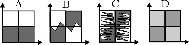
Figure 2: How a system evolves from step A to D in Fig.1 after a measurement error.

In 2A we have the same initial state as before. 2B shows the state just after the measurement was performed. Most of the initial states in the phase space are mapped to the correct final region, but a small fraction gets mapped to a different region. This corresponds to the cases where the result of the measurement does not agree with the actual position of the system molecule. If the system and the measurement device constitute an isolated system during the operation, and no other degrees of freedom are involved, the mapping from 2A to 2B would be described by a deterministic Hamiltonian evolution in time. Liouville’s theorem then guarantees that the entropy of the final state is the same as in the initial state. If the evolution is affected by other microscopic degrees of freedom in the device or the environment, which is certainly realistic in most cases, the mapping would be stochastic, and depend on these additional degrees of freedom. We can imagine that after B no further changes of the logical states will occur. That is, the phase point will never again cross the lines separating the different logical states. In a short time the phase space region where the system can be found will develop into some complicated shape 2C, but for a closed system the entropy will still be the same. Now we have to appeal to some coarse-graining procedure. For a closed system the phase-space coarse-graining introduced by Gibbs (see Ridderbos (2002) for a recent discussion). In the presence of some interaction with an environment, coarse-graining over dynamical evolution Blatt (1959); Lloyd (1989). In this way, the complex structure of the accessible phase space in 2C is rendered indistinguishable and replaced by the uniform distribution in 2D. This step is irreversible and increases the total entropy of the system by $S_{\epsilon}$ without any decrease in entropy anywhere.

To see the effect of the entropy production in each measurement, we will now analyze a model of an experimentally realized Szilard engine Koski et al. (2014). A single-electron-box (SEB) consisting of two metallic islands connected by a tunnel junction. The existence of an an additional electron on one of the two islands can be measured by the charge configuration of the box, and its state can be controlled by gate voltages applied to the islands, giving a time dependent potential difference $V(t)$ between the two islands. Work can be extracted from the system by the following procedure

1. Make the potential of the two islands equal, so that the probability of finding the extra electron is equal for the two islands.

2. Perform a measurement, and if the extra electron is found on one island, quickly raise the potential of the other island to some value $V_{0}\equiv V(0^{+})$.

3. Move the potential of the island back towards zero according to some protocol $V(t)$.

There is a probability that the electron will tunnel to the other island, taking energy from thermal fluctuations. Whenever the electron occupy this island while the potential is decreasing, heat is extracted from the environment and converted to work. A model equivalent to this was previously analyzed Bergli et al. (2013) when there was no errors in the measurements, and the consequences of reduced mutual information (but with no entropy production associated with the measurement) were discussed Horowitz and Parrondo (2011). We imagine that we are continuously repeating the above steps, and we want to minimize the total entropy production rate when varying the driving protocol $V(t)$ and the time $\tau$, at which we perform the next measurement and repeat the cycle. In the limit $\tau\rightarrow\infty$, corresponding to quasistatic operation, the entropy production will vanish if

$$\left(e^{V_{0}/T}+1\right)^{-1}=\epsilon.$$ (8)

as shown in Horowitz and Parrondo (2011). This means that the probabilities to find the electron on each of the islands are the same as if there was thermal equilibrium at this value of $V_{0}$.

While the entropy production rate can be zero when $\tau\rightarrow\infty$, we get a finite amount of work in an infinite time, which means that the power is zero. In Bergli et al. (2013) the problem of finding the $V(t)$ and $\tau$ minimizing the entropy production rate with a given power $P$ of heat taken from the reservoir was studied for the case $\epsilon=0$. If there is an error in the measurement, the feedback operation $V(t)$ will have to be adapted to the expected error rate to minimize the entropy production rate. Extending the analysis to finite $\epsilon$ is principally not difficult, the details are described in the Supplementary information. It leads to an ordinary nonlinear differential equation which has to be solved numerically. We now present the main results of this analysis. The model has a parameter $\Gamma$ which determines the tunneling rate between the two islands, and we measure time in units of $\Gamma^{-1}$ and energy in units of temperature $T$.

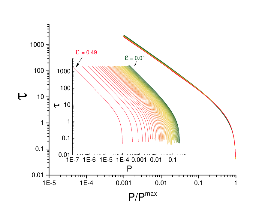
Figure 3: The inset shows $\tau$ as a function of $P$ for different $\epsilon$. The main figure gives the scaled form of the same data, with $\tau$ as a function of $P/P^{\max}$.

In Fig. 3 (inset) we plot the optimal period $\tau$ as a function of the power $P$ for selected values of the error $\epsilon$. We find that there is a maximal amount of power one can extract, $P^{\max}(\epsilon)$, as $\tau$ approaches 0. As $P$ approaches its maximum value $P^{\max}$ the period $\tau$ approaches 0 linearly: $\tau\propto P^{\max}-P$. As one might expect, when the power $P$ goes towards zero, the optimal period $\tau$ diverges to infinity. In other words, when we approach reversibility by performing the process in an infinite amount of time the power we can extract is zero. In the limit of low power $P\to 0$ we find that $\tau=\left(\ln 2-S_{\epsilon}\right)/P$, which we also confirm analytically in the supplement. We have found two curious facts: (i) To a very good approximation

$$P^{\max}(\epsilon)=\phi^{-1}(\epsilon-1/2)\sinh\left[\phi(\epsilon-1/2)\right],$$ (9)

where $\phi=1.618$ is the golden ratio. (ii) If $\tau$ is plotted as a function of $P/P^{\max}$ the scaled graphs are close to collapsing over the whole range of powers, as shown in Fig. 3.

The entropy production rate diverges as $\dot{S}\propto\left(P^{\max}-P\right)^{-1}$ when $P\rightarrow P^{\max}$, while it goes to zero for small $P$. In Ref. Bergli et al. (2013) it was found that for $\epsilon=0$ and small $P$, $\dot{S}$ is proportional to $P^{2}$. We find that this is not true for finite $\epsilon$. We expand to second order,

$$\dot{S}=c_{1}P+c_{2}P^{2},$$ (10)

where $c_{1}$ and $c_{2}$ are functions of $\epsilon$. Plotting $\dot{S}/P$ as a function of $P$ (Fig. 4) we get $c_{1}$ and $c_{2}$ as the intercept and slope of the tangent at $P=0$ (Fig. 4, inset).

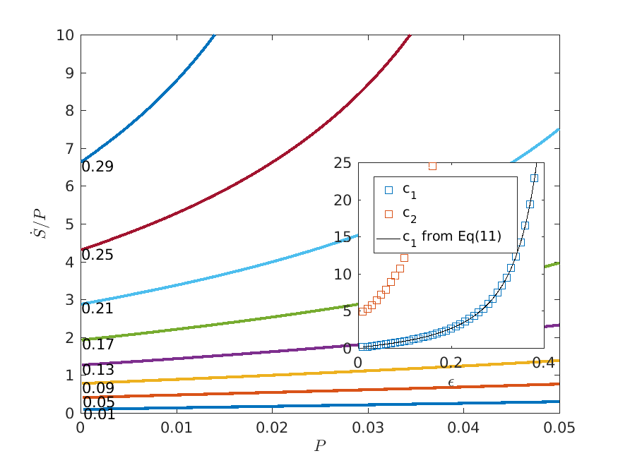
Figure 4: $\dot{S}/P$ as a function of $P$ with labels on the curves giving $\epsilon$. For each curve, the value at $P=0$ and the slope of the tangent at that point will give the coefficients $c_{1}$ and $c_{2}$ of Eq. (10). These are shown as functions of $\epsilon$ in the inset, together with $c_{1}$ from Eq. (11).

In agreement with Bergli et al. (2013) we find that $c_{1}$ goes to zero in the limit of $P\to 0$. The entropy production rate $\dot{S}$ is proportional to $P^{2}$ for error-free measurements, while it is proportional to $P$ if errors are present. In fact we can predict $c_{1}$ by using the asymptotic result $\tau=(\ln 2-S_{\epsilon})/P$. According to Eq. (10) of the supplement we have $\dot{S}=S_{\tau}/\tau-P$ where $S_{\tau}=-p_{\tau}\ln p_{\tau}-(1-p_{\tau})\ln(1-p_{\tau})$ is the entropy at time $\tau$ with $p_{\tau}$ the probability to find the electron on one of the islands at time $\tau$. It is reasonable, and also confirmed by the numerical solution of the optimization problem (see Supplement), that at small $P$ and long time $\tau$ the potential will be brought back to the initial value $V(\tau)=V_{0}$, so that final state will have equal probabilities for the electron to be found on either island, giving $S_{\tau}=\ln 2$. We then get

$$\dot{S}=c_{1}P\qquad\text{with}\qquad c_{1}=S_{\epsilon}(\ln 2-S_{\epsilon})^{-1},$$ (11)

which as shown in Fig. 4 (inset) agrees perfectly with the numerical solution.

Let us summarize the main results: if we make an error in a measurement, there is an associated net entropy production. This applies to measurements of any type and with an arbitrary number of outcomes. For a symmetric binary measurement where the probability of error is $\epsilon$, the entropy increases by the amount $S_{\epsilon}$. This entropy increase can be understood from a coarse-graining of either the phase space (for a closed system) or the dynamical evolutions (for an open system). We have investigated the consequences of a finite error on the optimal performance of a realistic Szilard engine at finite (given) power. We found the existence of a maximal power $P^{\max}$ which also exists for error-free measurements, and which decreases with increasing error. The entropy production rate diverges as the maximal power is approached. For small power, the entropy production rate is quadratic in $P$ in the absence of errors, but becomes linear when errors are present. We also found the driving protocol $V(t)$ and the time $\tau$ between measurements that minimize the entropy production.

I SUPPLEMENT

II I. Details of the model and Calculations

The model is the same as was studied previously Bergli et al. (2013) without measurement errors. Here we briefly repeat the necessary definitions. Let $p_{1}(t)$ and $p_{2}(t)$ be the probabilities to find the system in state 1 (the right island) and 2 (the left island), respectively. The transitions between these two states are described by the rates $\Gamma_{12}$ and $\Gamma_{21}$, which satisfy detailed balance $\Gamma_{21}/\Gamma_{12}=e^{\Delta E/T}$ (note that since $\Delta E$ is a function of time, the rates will also be time dependent). The master equations are thus

$$\dot{p}_{1} = -\Gamma_{12}p_{1}+\Gamma_{21}p_{2}=-\Gamma p_{1}+\Gamma_{21},$$

$$\dot{p}_{2} = \phantom{-}\Gamma_{12}p_{1}-\Gamma_{21}p_{2}=-\Gamma p_{2}+\Gamma_{12},$$ (12)

where $\Gamma(t)\equiv\Gamma_{12}(t)+\Gamma_{21}(t)$. As in Bergli et al. (2013) we choose for simplicity $\Gamma$ to be independent of time. The energy of state $i$ is denoted $E_{i}(t)$, and in the protocol described in the main text we have $E_{1}(t)=0$ and $E_{2}(t)=V(t)$. The total work extracted during the period $\tau$ is

$$W_{\text{ex}}=-\sum_{i=1}^{2}\int_{0}^{\tau}dt\,p_{i}\dot{E}_{i},$$ (13)

the change in internal energy of the system is

$$\Delta U=\sum_{i=1}^{2}\left[p_{i}(\tau)E_{i}(\tau)-p_{i}(0)E_{i}(0)\right],$$ (14)

and the transferred heat from the environment to the system is

$$Q=\Delta U+W_{\text{ex}}=\sum_{i=1}^{2}\int_{0}^{\tau}dt\,\dot{p}_{i}E_{i}(t).$$ (15)

The information entropy associated with the measurement is $H=-\sum_{i=1}^{2}p_{i}\ln p_{i}$, and the entropy production is therefore $\dot{H}=-\sum_{i=1}^{2}\dot{p}_{i}\ln p_{i}$. The change in information entropy can be written as an integral

$$\Delta H=-\sum_{i=1}^{2}\int_{0}^{\tau}dt\,\dot{p}_{i}\ln p_{i}.$$ (16)

Since $p_{1}=1-p_{2}$, we can relabel $p_{2}\equiv p$, and write the entropy produced per cycle as

$$\frac{\Delta H}{\tau} = -\frac{1}{\tau}\int_{0}^{\tau}dt~{}\dot{p}\ln\left(\frac{p}{1-p}\right).$$ (17)

The master equation (II) can be expressed as

$$\dot{p}=-p+\frac{1}{e^{V}+1}$$ (18)

where from now on we will measure time in units of $\Gamma$ and energy in units of $T$. From this equation we can express

$$V=\ln\left(\frac{1}{p+\dot{p}}-1\right).$$

The power is defined as the average heat extracted from the reservoir per cycle $\tau$, $P=Q/\tau$, and can be written as

$$P=\frac{1}{\tau}\int_{0}^{\tau}dt~{}\dot{p}V=\frac{1}{\tau}\int_{0}^{\tau}dt~{}\dot{p}~{}\ln\left(\frac{1}{p+\dot{p}}-1\right).$$ (19)

We are interested in the optimal protocol for the measurement and erasure cycle. In this system the optimal protocol means finding the protocol $V(t)$ and the total time $\tau$ we should use on the cycle, that minimize the entropy production rate given a measurement error $\epsilon\in[0,\,1]$ and a desired power $P$. The total entropy production rate for perfect measurements is

$$\frac{\Delta S_{\text{tot}}}{\tau}=\frac{\Delta H}{\tau}-P.$$ (20)

To study the effect of measurement errors, we have to add the entropy produced in the measurement, $S_{\epsilon}=-\epsilon\ln\epsilon-(1-\epsilon)\ln(1-\epsilon)$, as discussed in the main text:

$$\frac{\Delta S_{\text{tot}}}{\tau}=\frac{\Delta H}{\tau}+\frac{S_{\epsilon}}{\tau}-P.$$ (21)

We are interested in solutions where the power is given by a finite non-zero value, given by Eq. (19).

The initial condition is $p(t=0)=\epsilon$. That is, there is a chance, $\epsilon$, that the electron was on the island where the potential was raised from $V(0)=0$ to $V(0^{+})=V_{0}$, and thus preforming work on the system. We also set the value of the power, $P$, to see how the solutions depend on the power we want to extract.

Since $S_{\epsilon}$ is a constant value that depends only on the initial condition, it is sufficient to minimize the information entropy given in Eq. (17). Since we want to minimize it while keeping the power at a finite value $P$, we have to introduce the Lagrange multiplier $\lambda$ to obtain the functional

$$I=\frac{\Delta H}{\tau}+\lambda P=\frac{1}{\tau}\int_{0}^{\tau}dt~{}L(p,\dot{p},\lambda),$$ (22)

with the Lagrangian

$$L(p,\dot{p},\lambda)=\left[-\ln\left(\frac{p}{1-p}\right)+\lambda\ln\left(\frac{1}{\dot{p}+p}-1\right)\right]\dot{p}.$$ (23)

Using the Euler-Lagrange equation

$$\frac{\partial L}{\partial p}=\frac{\partial}{\partial t}\frac{\partial L}{\partial\dot{p}}$$ (24)

we obtain the following second-order nonlinear ordinary differential equation:

$$\ddot{p}=\frac{\dot{p}^{2}(\dot{p}+p-1/2)}{p(\dot{p}+p-1)+\dot{p}/2}\,.$$ (25)

In order to solve this equation we need to impose a set of constraints to the solutions we want. The first constraint is that the power has to be a finite fixed value $P$, given by Eq. (19):

$$G(\tau,p,\dot{p})\equiv P-\frac{1}{\tau}\int_{0}^{\tau}dt~{}\dot{p}\ln\left(\frac{1}{p+\dot{p}}-1\right)=0.$$ (26)

The second constraint comes from a consideration of the endpoint values of $p(t)$. The initial condition of $p(t)$ is given by $p(0)=\epsilon$, but since the value of $p(t)$ is not fixed at the endpoint $p(\tau)$ we have a second constraint, $(\partial L/\partial\dot{p})_{t=\tau}=0$, which can be written as

$$F_{1}\left(\lambda,\tau,p\right)\equiv \lambda\left[\ln\left(\frac{1}{p+\dot{p}}-1\right)+\frac{\dot{p}}{(\dot{p}+p-1)(\dot{p}+p)}\right]$$ (27)

$$-\ln\left(\frac{p_{\tau}}{1-p_{\tau}}\right)=0.$$

The third and final constraint is due to the fact that variation of Eq. (21) with respect to the period $\tau$ should be zero. It is given by

$$\frac{\partial\Delta S_{\text{tot}}}{\partial\tau}=\lambda\frac{\partial P}{\partial\tau}-\frac{1}{\tau^{2}}\left(\Delta H+S_{\epsilon}\right)+\frac{1}{\tau}\frac{\partial S_{\tau}}{\partial\tau}=0$$ (28)

where

$$\frac{\partial P}{\partial\tau} = \frac{\partial}{\partial\tau}\left[\frac{1}{\tau}\int_{0}^{\tau}dt~{}\dot{p}~{}\ln\left(\frac{1}{p+\dot{p}}-1\right)\right]$$ (29)

$$= \frac{\dot{p}_{\tau}}{\tau}\ln\left(\frac{1}{p_{\tau}+\dot{p}_{\tau}}-1\right)-\frac{P}{\tau},$$

and

$$\frac{\partial}{\partial\tau}\frac{\Delta H}{\tau} = \frac{\partial}{\partial\tau}\left[-\frac{1}{\tau}\int_{0}^{\tau}dt~{}\dot{p}\ln\left(\frac{p}{1-p}\right)\right]$$ (30)

$$= \frac{1}{\tau}\dot{p}_{\tau}\ln\left(\frac{1-p_{\tau}}{p_{\tau}}\right)-\frac{\Delta H}{\tau^{2}}.$$

The full equation for the third constraint is thus

$$F_{2}(\lambda,\tau,p) \equiv \left[\ln\left(\frac{1-p_{\tau}}{p_{\tau}}\right)+\lambda\dot{p}_{\tau}\ln\left(\frac{1}{p_{\tau}+\dot{p}_{\tau}}-1\right)\right]$$ (31)

$$- \lambda P-\frac{1}{\tau}\left[\Delta H+S_{\epsilon}\right]=0,$$

This constraint can be combined with the free-endpoint constraint by eliminating the Lagrange multiplier $\lambda$ to obtain

$$F\left(\tau,p_{\tau},\dot{p}_{\tau}\right)\equiv\ln\left(\frac{p_{\tau}}{1-p_{\tau}}\right)\left[P(\dot{p}_{\tau}+p_{\tau})(p_{\tau}+\dot{p}_{\tau}-1)\right.$$

$$\left.\qquad+\dot{p}^{2}_{\tau}\right]-\frac{S_{\tau}}{\tau}\left[\dot{p}_{\tau}+\ln\left(\frac{1}{p_{\tau}+\dot{p}_{\tau}}-1\right)\right.$$

$$\left.\qquad\qquad\times(\dot{p}_{\tau}+p_{\tau})(p_{\tau}+\dot{p}_{\tau}-1)\right]=0,$$ (32)

where $S_{\tau}=\Delta H+S_{\epsilon}=-p_{\tau}\ln p_{\tau}-(1-p_{\tau})\ln(1-p_{\tau})$ is the entropy of system at time $t=\tau$.

It may seem surprising that the Lagrange multiplier $\lambda$ disappears in the solution to the Euler-Lagrange equation, but this is because the entropy term in Eq. (17) is a complete integral. It is of course a state-function, that only depends of the initial and final values of $p(t)$.

$$\Delta S = -\int_{0}^{\tau}dt~{}\dot{p}\ln\left(\frac{p}{1-p}\right)=-\int_{0}^{\tau}dp~{}\ln\left(\frac{p}{1-p}\right)$$ (33)

$$= \bigg{[}-p\ln p-(1-p)\ln(1-p)\bigg{]}_{0}^{\tau}=S_{\tau}-S_{0}.$$

We use Euler’s method to solve the second order differential equation in Eq. (25). Since it is a second order equation we have two constants that needs to be fixed ($\tau$ and $V_{0}$). We find these values as the roots of the two constraints in Eq. (26) and Eq. (32) by using Newton’s method.

III II. Additional results

Here we present some additional results on the optimal protocol.

III.1 The protocol $V(t)$

The exact form of the function $V(t)$ which minimizes the entropy production can only be found from the numerical solution of Eq. (25). However, some limiting cases and the dependence on the parameters $\epsilon$ and $P$ can be understood to some extent. The numerical solution for $V(t)$ is shown in Fig. 5

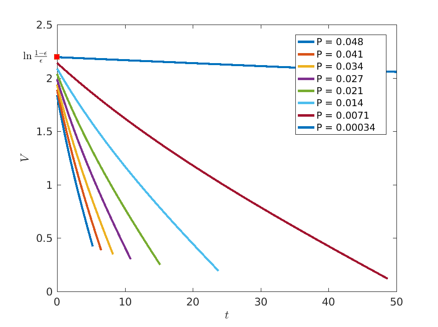
Figure 5: $V(t)$ for $\epsilon=0.1$ and several values of $P$.

for $\epsilon=0.1$ and several values of $P$. We observe several facts: i) The time $\tau$ before the protocol should be repeated decreases with increasing $P$. ii) The initial value $V_{0}$ increases with decreasing $P$. In the limit $P\rightarrow 0$, we should have according to Eq. (8) of the main text $V_{0}=\ln\frac{1-\epsilon}{\epsilon}$, which is marked in the figure. We see that the numerical results agree with this prediction. iii) The final value $V_{\tau}=V(\tau)$ depends on $P$ and goes to zero for small $P$.

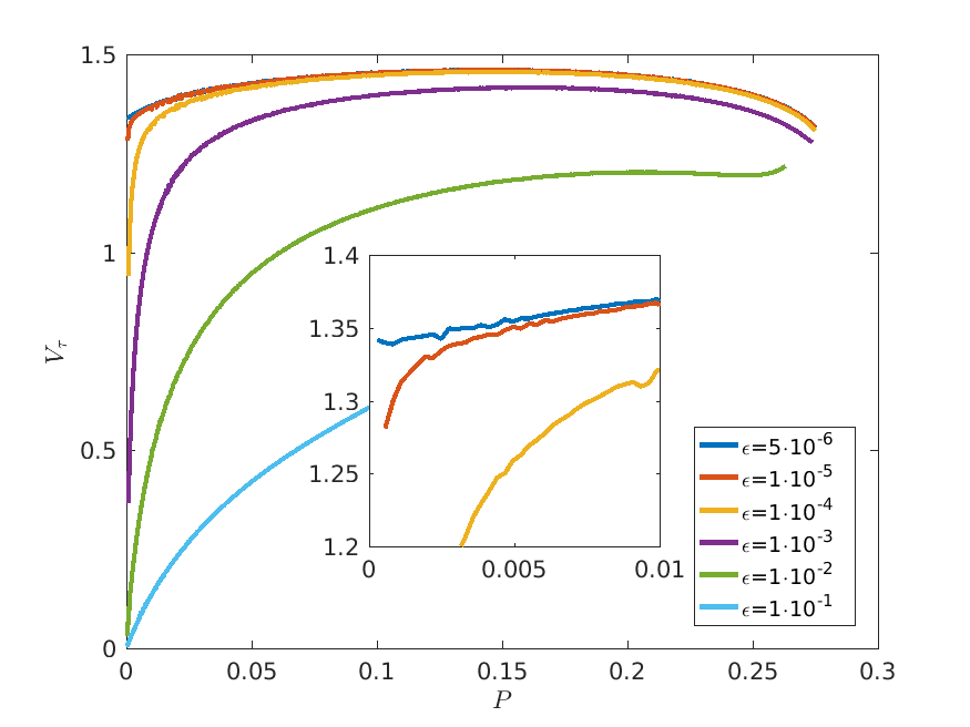
Figure 6: $V_{\tau}$ as function of $P$ for different $\epsilon$. The inset shows enlarged what happens for small errors and powers.

Figure 6 shows $V_{\tau}$ as function of $P$ for different $\epsilon$. While it seems that for any finite $\epsilon$ we find $V_{\tau}\rightarrow 0$ as $P\rightarrow 0$, we see that for small $\epsilon$ one has to go to very small powers to see this, and for most power $V_{\tau}$ is between 1 and 1.5. This indicates a singular behaviour of the function $V_{\tau}(P,\epsilon)$ at $P=0$ and $\epsilon=0$, and the limiting value will depend on how this point is approached. In Bergli et al. (2013) we found that $V_{\tau}=1.33$ for $\epsilon=0$ and small $P$. From Fig. 6 (inset) we can see that this agrees well with what we would expect if we first took the limit $\epsilon\rightarrow 0$ and then $P\rightarrow 0$. The same singularity is reflected in the probability $p_{\tau}$ to find the electron on the opposite island at time $\tau$ from the one it was measured at time 0 as shown in Fig. 7. For all finite $\epsilon$ we have $\lim_{P\rightarrow 0}p_{\tau}=0.5$, but for small $\epsilon$ this only happens at very small $P$.

Figure 7: $p_{\tau}$ as function of $P$ for different $\epsilon$

III.2 The maximal power, $P^{\max}$

We can always find the value of $P^{\max}$ from the numerical solution of Eqs. (25), (26), (32) by determining when $\tau$ becomes 0. But we can also derive a single transcendental equation which determines $P^{\max}$ , and in the case of error-free measurements we can also solve it analytically.

By taking the limit as $\tau\to 0$ in Eq. (19) we find that

$$P^{\max}=V_{0}\dot{p}_{0}=V_{0}\left(\frac{1}{e^{V_{0}}+1}-\epsilon\right).$$ (34)

which expresses $P^{\max}$ in terms of $V_{0}$. Consider Eq. (32) when $\tau\rightarrow 0$. Since the other terms are finite, the only way to avoid a divergence of the last term is that expression in brackets is zero. For $\tau=0$ we have $p_{\tau}=\epsilon$ and with Eq. (18) we find that $V_{0}$ satisfies the equation

$$1+(1-V_{0})e^{V_{0}}-\epsilon(e^{V_{0}}+1)^{2}=0.$$ (35)

For $\epsilon=0$ we find that the maximum power is given by the Lambert W function

$$P^{\max}=W(e^{-1})=0.27846\dots$$ (36)

with the initial value of the potential $V_{0}=1+W(e^{-1})$. This analytical result is in perfect agreement with our numerical one.

Curiously, a good approximation to this plot is given by

$$P^{\max}=\frac{\epsilon-1/2}{\phi}\sinh\left(\phi(\epsilon-1/2)\right).$$ (37)

The difference between the true and approximate solution is only $10^{-4}$ for $\epsilon=0$:

$$P^{\max}=\frac{1}{2\phi}\sinh\left(\frac{\phi}{2}\right)=0.27817\dots$$ (38)

III.3 The dependence of $\tau$ on $P$ for small $P$

When $P=0$ we can assume the system to always be in equilibrium at the given value of $V$, which means that $p=p_{a}=\left(e^{V}+1\right)^{-1}$. We assume for small $P$ we have $p=p_{a}+\mathcal{O}(P)$, and that $\tau=A/P$. Inserting into Eq. (19) and expanding in $P$ we find that it becomes

$$1=\frac{1}{A}\int_{0}^{\infty}dtV\dot{p}_{a}+\mathcal{O}(P)$$

Using the fact found above that $V(\infty)=\lim_{P\rightarrow 0}V_{\tau}=0$ (at leat for finite $\epsilon$) and that $\lim_{P\rightarrow 0}V_{0}=\ln\frac{1-\epsilon}{\epsilon}$, we get

$$A=\int_{0}^{\infty}dtV\dot{p}_{a}=-\int_{0}^{V_{0}}dVV\frac{dp_{a}}{dV}=\ln 2-S_{\epsilon}$$