Low-Resolution Near-infrared Stellar Spectra Observed by the Cosmic Infrared Background Experiment (CIBER)

Abstract

We present near-infrared (0.8-1.8 $\micron$) spectra of 105 bright (${m_{J}}$ $<$ 10) stars observed with the low resolution spectrometer on the rocket-borne Cosmic Infrared Background Experiment (CIBER). As our observations are performed above the earth’s atmosphere, our spectra are free from telluric contamination, which makes them a unique resource for near-infrared spectral calibration. Two-Micron All Sky Survey (2MASS) photometry information is used to identify cross-matched stars after reduction and extraction of the spectra. We identify the spectral types of the observed stars by comparing them with spectral templates from the Infrared Telescope Facility (IRTF) library. All the observed spectra are consistent with late F to M stellar spectral types, and we identify various infrared absorption lines.

1 Introduction

Precise ground-based measurements of stellar spectra are challenging in the near-infrared (IR) because of the contaminating effects of telluric lines from species like water, oxygen, and hydroxyl in the earth’s atmosphere. Telluric correction using standard stars is generally used to overcome this problem, but these corrections are problematic in wavelength regions marked by strong line contamination, such as from water and hydroxyl. In contrast, space-based spectroscopy in the near-IR does not require telluric correction, so can provide new insights into stellar atmospheres (e.g. Matsuura et al. 1999; Tsuji et al. 2001), especially near $1\micron$ where starlight is not reprocessed by dust in the circumstellar environment (Meyer et al., 1998). In particular, near-IR spectra can be used to study the age and mass of very young stars (Joyce et al., 1998; Peterson et al., 2008), and the physical properties of very cool stars (Sorahana & Yamamura, 2014).

Of particular interest in the study of the atmospheres of cool stars is water. According to early models of stellar photospheres (Russell, 1934), H₂O existed only in later than M6 type stars, and until recently observations have supported this. In 1963, the balloon-borne telescope Stratoscope II observed H₂O in two early M2-M4 giant stars (Woolf et al., 1964) at 1.4 and $1.9\,\micron$. Several decades later, Tsuji et al. (1997) measured H₂O absorption in an M2.5 giant star using the Infrared Space Observatory (Kessler et al. 1996), and Matsuura et al. (1999) observed water at 1.4, 1.9, 2.7, and $6.2\micron$ for 67 stars with the Infrared Telescope in Space (Murakami et al. 1996; Matsumoto et al. 2005). Surprisingly, Tsuji et al. (2001) discovered water features in late K-type stars. These results required a new stellar photosphere model to explain the existence of H₂O features in hotter than M6 type stars (Tsuji et al., 2015).

The low resolution spectrometer (LRS; Tsumura et al. 2013) on the Cosmic Infrared Background Experiment (CIBER; Bock et al. 2006; Zemcov et al. 2013) observed the diffuse infrared background from 0.7 to 2.0 $\micron$ during four flights above the Earth atmosphere. The LRS was designed to observe the near-IR background (Hauser & Dwek, 2001; Madau & Pozzetti, 2000), and as a result finds excess extragalactic background light above all known foregrounds (Matsuura et al. 2016, ApJ, submitted, 2016). Furthermore, we precisely measure astrophysical components contributing to the diffuse sky brightness (see Leinert et al. 1998 for a review). For example, Tsumura et al. (2010) observed a component of the zodiacal light absorbed by silicates in a broad band near $800\,$nm. By correlating the LRS with a 100 $\micron$ dust map (Schlegel, 1998), Arai et al. (2015) measured smooth diffuse galactic light spectrum from the optical band to the near-IR and constrained the size distribution of interstellar dust, which was dominated by small particles (half-mass radius $\sim$0.06 $\micron$).

The LRS also observed many bright galactic stars, enabling us to study their near-IR SEDs. In this paper, we present flux-calibrated near-IR spectra of 105 stars from $0.8\leq\lambda\leq 1.8\,\micron$ with spectral resolution $15\leq\lambda/\Delta\lambda\leq 30$ over the range. The paper is organized as follows. In Section 2, the observations and instrumentation are introduced. We describe the data reduction, calibration, astrometry, and extraction of the stellar spectra in Section 3. In Section 4, the spectral typing and features are discussed. Finally, a summary and discussion are given in Section 5.

2 Instrument

The LRS is one of the four optical instruments of the CIBER payload (Zemcov et al., 2013); the others are a narrowband spectrometer (Korngut et al. 2013) and two wide-field imagers (Bock et al., 2013). The LRS (Tsumura et al., 2013) is a prism-dispersed spectrometer with five rectangular $5.35^{\circ}\times 2.8\arcmin$ slits imaging a 5.8 ^∘ $\times$ 5.8 ^∘ field of view. The detector has $256\times 256$ pixels at a pixel scale of $1.36\arcmin\times 1.36\arcmin$. CIBER has flown four times (2009 February, 2010 July, 2012 March, and 2013 June) with apogees and total exposure times of over 325 km and $\sim$ 240 s, respectively, in the first three flights and of 550 km and 335 s in the final, non-recovered flight. Due to spurious signal contamination from thermal emission from the shock-heated rocket skin, we do not use the first flight data in this work (Zemcov et al., 2013). Eleven target fields were observed during the three subsequent flights, as listed in Table 1. Details of the field selection are described in Matsuura et al. 2016, ApJ, submitted (2016).

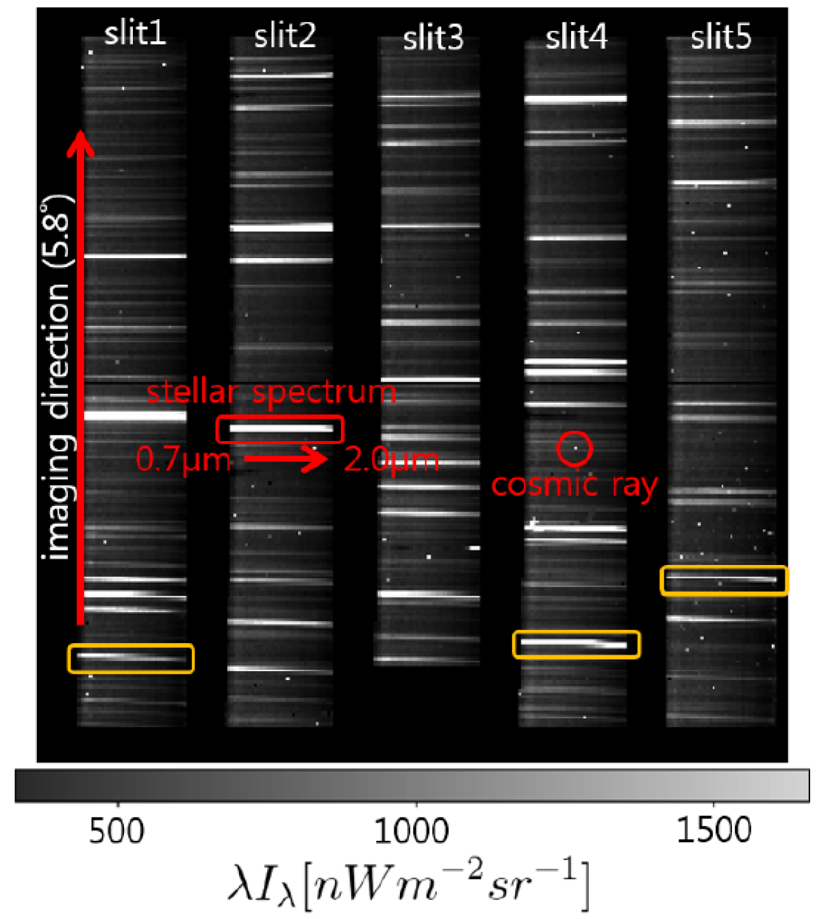
Figure 1: An example CIBER-LRS image toward the NEP field. The five illuminated columns are dispersed spectra from the five slits of the LRS, and the bright horizontal lines in each column are images of individual stars. As an example, we highlight a single horizontal light trail by a red box; this is the light from a single star dispersed from 0.7 to 2.0 $\micron$. The bright dots are pixels hit by cosmic rays. The yellow boxes highlight representative examples of stellar spectra disturbed by the prism. Note that the distortion direction is different between the upper and lower parts of the image, and the distortion becomes negligible at the center line of the image.

During the observations, the detector array is read nondestructively at $\sim 4\,$Hz frame^-1. Each field is observed for many tens or hundreds of frames, and an image for each field is obtained by computing the slope of the accumulated values for each pixel (Garnett & Forrest, 1993). Figure 1 shows an example image of the North Ecliptic Pole (NEP) region obtained during the second flight. More than 20 bright stars ($m_{J}$ $<$ 11) are observed. The stellar spectra are characterized by a small amount of field distortion as well as an arc-shaped variation in constant-wavelength lines along the slit direction. The latter is known as a “smile” and is a known feature of prism spectrometers (Fischer et al., 1998). Details of the treatment of these distortions are described in Section 3.3 and 3.4.

3 Data Analysis

In this section, we describe how we perform background subtraction, calibration, photometric estimation, astrometric registration, and spectral extraction from the LRS-observed images.

3.1 Pixel response correction

We measure the relative pixel response (flat field) in the laboratory before each flight (Arai et al., 2015). The second- and the third-flight data are normally corrected with these laboratory flats. However, for the fourth flight from the laboratory calibrations do not extend to the longest wavelengths ($\lambda\geq 1.4\micron$) because the slit mask shifted its position with respect to the detector during the flight. We therefore use the second-flight flat field to correct the relative response for the fourth-flight data, as this measurement covers $\lambda>1.6\micron$. To apply this flat field, we need to assume that the intrinsic relative pixel response does not vary significantly over the flights. To check the validity of this assumption, we subtract the second flat image to the fourth flat image for overlapped pixels and calculate the pixel response difference. We find that only 0.3 % of pixels with response measured in both are different by $2\sigma$, where $\sigma$ is the standard deviation of the pixel response. Finally, we mask 0.06 % of the array detectors to remove those pixels with known responsivity pathologies and those prone to transient electronic events (Lee et al., 2010).

3.2 Calibration

For each flight, the absolute brightness and wavelength irradiance calibrations have been measured in the laboratory in collaboration with the National Institute of Standards and Technology. The details of these calibrations can be found in Tsumura et al. (2013). The total photometric uncertainty of the LRS brightness calibration is estimated to be $\pm 3$% (Tsumura et al., 2013; Arai et al., 2015).

3.3 Background Removal

The raw image contains not only spectrally dispersed images of stars but also the combined emission from zodiacal light $\lambda I_{\lambda}^{\rm ZL}$, diffuse galactic light $\lambda I_{\lambda}^{\rm DGL}$, the extragalactic background $\lambda I_{\lambda}^{\rm EBL}$, and instrumental effects $\lambda I_{\lambda}^{\rm inst}$ (Leinert et al., 1998). The measured signal $\lambda I_{\lambda}^{\rm meas}$ can be expressed as

$$\lambda I_{\lambda}^{\rm meas}=\lambda I_{\lambda}^{\ast}+\lambda I_{\lambda}^{\rm ZL}+\lambda I_{\lambda}^{\rm ISL}+\lambda I_{\lambda}^{\rm DGL}+\lambda I_{\lambda}^{\rm EBL}+\lambda I_{\lambda}^{\rm inst},$$ (1)

where we have decomposed the intensity from stars into a resolved component $\lambda I_{\lambda}^{\ast}$ and an unresolved component arising from the integrated light of stars below the sensitivity of the LRS $\lambda I_{\lambda}^{\rm ISL}$. It is important to subtract the sum of all components except $\lambda I_{\lambda}^{\ast}$ from the measured brightness to isolate the emission from detected stars. At this point in the processing, we have corrected for multiplicative terms affecting $\lambda I_{\lambda}^{\rm meas}$. Dark current, which is the detector photocurrent measured in the absence of incident flux, is an additional contribution to $\lambda I_{\lambda}^{\rm inst}$. The stability of the dark current in the LRS has been shown to be 0.7 nW m^-2 sr^-1 over each flight, which is a negligible variation from the typical dark current (i.e., 20 nW m^-2 sr^-1; (Arai et al., 2015)). As a result, we subtract the dark current as part of the background estimate formed below.

The relative brightnesses of the remaining background components are wavelength-dependent, so an estimate for their mean must be computed along constant-wavelength regions, corresponding to the vertical columns in Figure 1. Furthermore, because of the LRS’s large spatial PSF, star images can extend over several pixels in the imaging direction and even overlap one another. This complicates background estimation in pixels containing star images and reduces the number of pixels available to estimate the emission from the background components.

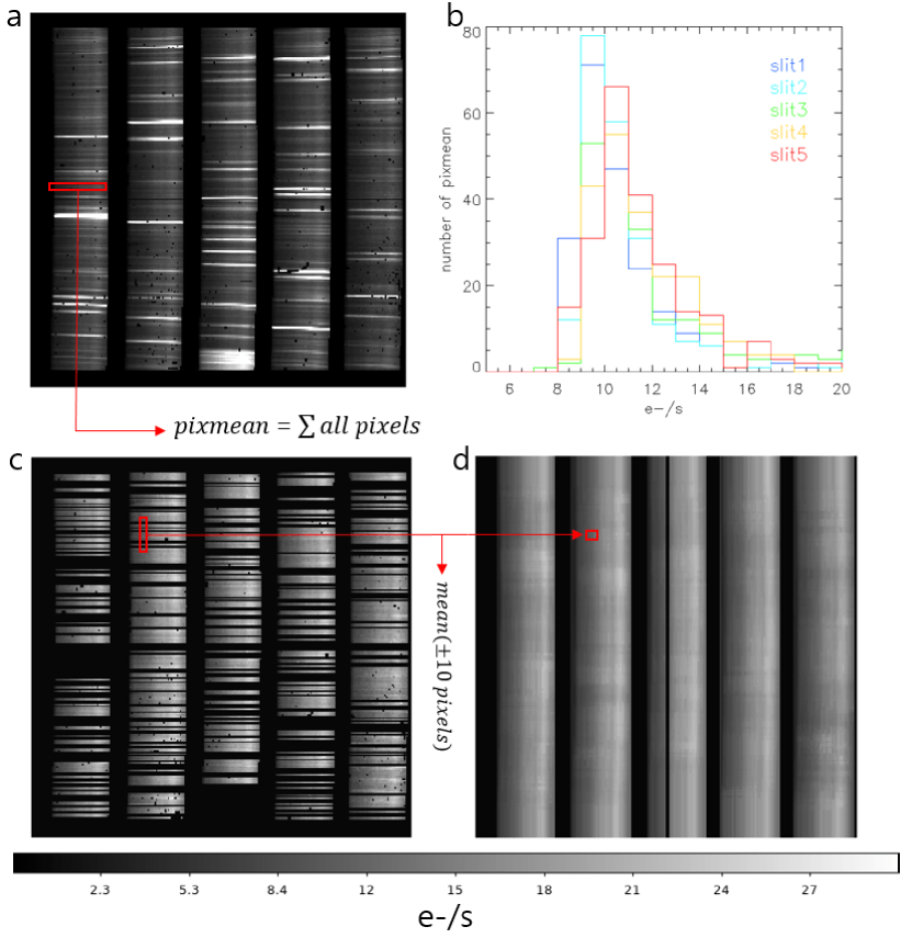
Figure 2: Flow chart of the background image construction. (a) Same as Figure 1. The red box indicates the set of rows to be averaged. (b) Histogram of averaged values for each row. This average values for each slit are drawn with different color. (c) Image after iterative sigma clipping of bright rows from (b). The red box indicates the size of $\pm$ 10 pixels that are averaged. (d) Reconstructed background image including all instrumental noise and undetected faint stars.

To estimate the background in those pixels containing star images, we compute the average value of pixels with no star images along each column, as summarized in Figure 2. We remove bright pixels that may contain star images, as described in Arai et al. (2015). The spectral smile effect shown in Figure 1 introduces spectral curvature along a column. We estimate it causes an error of magnitude $\delta\lambda/\lambda<10^{-2}$, which is small compared to the spectral width of a pixel. Approximately half of the rows remain after this clipping process; the fraction ranges from 45 % to 62 % depending on the stellar density in each field. This procedure removes all stars with $J>13$, and has a decreasing completeness above this magnitude (Arai et al., 2015).

To generate an interpolated background map, each candidate star pixel is replaced by the average of nearby pixels calculated along the imaging direction from the $\pm 10$ pixels on either side of the star image. We again do not explicitly account for the spectral smile. This interpolated background image is subtracted from the measured image, resulting in an image containing only bright stellar emission. The emission from faint stars and bright stars that inefficiently illuminate a grating slit that contributes to $I_{\lambda}^{\rm ISL}$ is naturally removed in this process.

3.4 Star Selection

The bright lines dispersed in the spectral direction in the background-subtracted images are candidate star spectra. To calculate the spectrum of candidate sources, we simply isolate individual lines of emission and map the pixel values onto the wavelength using the ground calibration. However, this procedure is complicated both by the extended spatial PSF of the LRS and by source confusion.

To account for the size of the LRS spatial PSF (FWHM $\sim$1.2 pixels) as well as optical distortion from the prism that spreads the star images slightly into the imaging direction, we sum five rows of pixels in the imaging direction for each candidate star. Since the background emission has already been accounted for, this sum converges to the total flux as the number of summed rows is increased. By summing five rows, we capture $>99.9$% of a candidate star’s flux. The wavelengths of the spectral bins are calculated from the corresponding wavelength calibration map in the same way.

From these spectra, we can compute synthetic magnitudes in the $J$- and $H$-bands, which facilitate comparison to Two-Micron All-Sky Survey (2MASS) measurements. We first convert surface brightness in nW m^-2 sr^-1 to flux in nW m^-2 Hz^-1, and then integrate the monochromatic intensity over the 2MASS band, applying the filter transmissivity of the $J$- and $H$-bands (Cohen et al., 2003). To determine the appropriate zero magnitude, we integrate the $J$- and $H$-band intensity of Vega’s spectrum (Bohlin & Gilliland, 2004) with the same filter response. The $J$- and $H$-band magnitudes of each source are then calculated, allowing both flux and color comparisons between our data and the 2MASS catalog.

Candidate star spectra may be comprised of the blended emission from two or more stars, and these must be rejected from the catalog. Such blends fall into one of two categories: (i) stars that are visually separate but are close enough to share flux in a 5 pixel-wide photometric aperture, and (ii) stars that are close enough that their images overlap so as to be indistinguishable. We isolate instances of case (i) by comparing the fluxes calculated by summing both three and five rows along the imaging direction for each source. If the magnitude or $J-H$ color difference between the two apertures is larger than the statistical uncertainty (described in Section 3.6), we remove those spectra from the catalog. To find instances of case (ii), we use the 2MASS star catalog registered to our images using the procedure described in Section 3.5. Candidate sources that do not meet the criteria presented below are rejected.

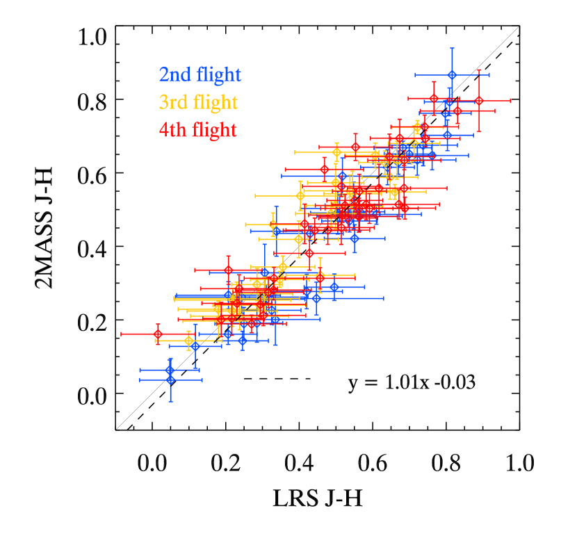
Figure 3: LRS J-H color comparison with cross-matched 2MASS J-H color. Each color corresponds to a different flight. The dashed line shows a linear fit, exhibiting a slight systematic offset from unity. The J-H colors of LRS stars are conserved regardless of the slit apodization effect.

To ensure the catalog spectra are for isolated stars rather than for indistinguishable blends, we impose the following requirements on candidate star spectra: (i) each candidate must have $J<11$; (ii) the $J$-band magnitude difference between the LRS candidate and the matched 2MASS counterpart must be $<1.5$; (iii) the $J-H$ color difference between the LRS candidate star and the matched 2MASS counterpart must be $<0.3$; and (iv) among the candidate 2MASS counterparts within the 500$\arcsec$ ($=6$ pixel) radius of a given LRS star, the second-brightest 2MASS star must be fainter than the brightest one by more than 2 mag at the J band. Criterion (i) excludes faint stars that may be strongly affected by residual backgrounds, slit mask apodization, or source confusion. The second and third criteria mitigate mismatching by placing requirements on the magnitude and color of each star. In particular, the $J-H$ color of a source does not depend on the slit apodization or the position in image space (see Figure 3), so any significant change in $J-H$ color as the photometric aperture is varied suggests that more than a single star could be contributing to the measured brightness. Finally, it is possible that two stars with similar $J-H$ colors lie close to each other, so the last criterion is applied to remove stars for which equal-brightness blending is an issue. Approximately one in three candidate stars fails criterion (iv). The number of candidate stars rejected at each criterion is described in Table 2.

In addition, three of LRS candidate stars are identified as variables in the SIMBAD database . We also identify two stars as binary and multiple-star systems as well as four high proper motion stars. Through these stringent selection requirements, we conservatively include only the spectra of bright, isolated stars in our catalog. Finally, 105 star spectra survive all the cuts, and the corresponding stars are selected as catalog members.

3.5 Astrometry

We match the synthesized LRS $J$, $H$, and $J-H$ information with the 2MASS point source catalog (Skrutskie et al., 2006) to compute an astrometric solution for the LRS pointing in each sky image. This is performed in a stepwise fashion by using initial estimates for the LRS’s pointing to solve for image registration on a fine scale.

As a rough guess at the LRS pointing, we use information provided by the rocket’s attitude control system (ACS), which controls the pointing of the telescopes (Zemcov et al., 2013). This provides an estimated pointing solution that is accurate within 15 $\arcmin$ of the requested coordinates. However, since the ACS and the LRS are not explicitly aligned to one another, a finer astrometric registration is required to capture the pointing of the LRS to single-pixel accuracy.

To build a finer astrometric solution, we simulate images of each field in the 2MASS J-band using the positional information from the ACS, spatially convolved to the LRS PSF size. Next, we apodize these simulated 2MASS images with the LRS slit mask, compute the slit-masked magnitudes of three reference stars, and calculate the $\chi^{2}$ statistic using

$$\chi^{2}{{}_{p,q}}=\sum_{i}\left(\frac{F_{LRS,i}-F_{2MASS,i}}{\sigma_{LRS,i}}\right)^{2},$$ (2)

where index i represents each reference star and subscripts p and q index the horizontal and vertical positions of the slit mask, respectively. $F_{LRS,i}$ and $F_{2MASS,i}$ are the fluxes in the LRS and 2MASS $J$-band, and $\sigma_{LRS,i}$ is the statistical error of the LRS star (see Section 3.6). The minimum $\chi^{2}$ gives the most likely astrometric position of the slit mask. Since, on average, there are around five bright stars with $J<9$ per field, spurious solutions are exceedingly unlikely, and all fields give a unique solution.

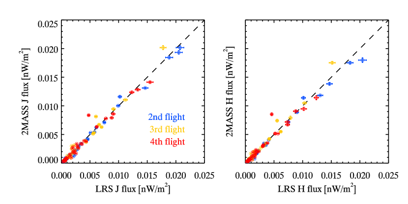
Figure 4: The 2MASS J- and H-band fluxes are shown as a function of the LRS J- and H-band. Each color represents the data obtained on a different flight. Slit apodization effect is corrected for all LRS stars. Correction factors are derived based on the slit simulation for magnitude ranges covered by the LRS stars, as shown in Figure 10 and 11.

Using this astrometric solution, we can assign coordinates to the rest of the detected LRS stars. We estimate that the overall astrometric error is 120$\arcsec$ by computing the mean distance between the LRS and 2MASS coordinates of all matched stars. The error corresponds to 1.5 times the pixel scale. We check the validity of the astrometric solutions by comparing the colors and fluxes between the LRS and matched 2MASS stars. In Figures 3 and 4, we show the comparison of the $J-H$ colors and fluxes of the cross-matched stars in each field. Here, we multiply the LRS fluxes at the J- and H-band by 2.22 and 2.17, respectively, to correct for the slit apodization. The derivation of correction factors is described in Section 5. On the whole, they match well within the error range.

3.6 Spectral Error Estimation

Even following careful selection, the star spectra are subject to various kinds of uncertainties and errors, including statistical uncertainties, errors in the relative pixel response, absolute calibration errors, wavelength calibration errors, and background subtraction errors.

Statistical uncertainties in the spectra can be estimated directly from the flight data. We calculate the $1\sigma$ slope error from the line fit (see Section 2) as we generate the flight images; this error constitutes the estimate for the statistical photometric uncertainty for each pixel. In this statistical error, we include contributions from the statistical error in the background estimate and the relative pixel response. The error in the background signal estimate is formed by computing the standard deviation of the $\pm$10 pixels along the constant-$\lambda$ direction for each pixel to match the background estimate region. This procedure captures the local structure in the background image, which is a reasonable measure of the variation we might expect over a photometric aperture. Neighboring pixels in the wavelength direction have extremely covariant error estimates in this formulation, which are acceptable since the flux measurements are also covariant in this direction. A statistical error from the relative pixel response correction is applied by multiplying 3% of the relative response by the measured flux in each field (Arai et al., 2015). To compute the total statistical error, each constituent error is summed in quadrature for each pixel.

Several instrumental systematic errors are present in these measurements, including those from wavelength calibration, absolute calibration, and relative response correction. In this work, we do not explicitly account for errors in the wavelength calibration, as the variation is $\pm$ 1 nm over 10 constant-wavelength pixels, which is $<0.1R$. In all flights, $<$ 3 % absolute calibration error is applied (Arai et al., 2015). For the longest-wavelength regions ($\lambda$ $>$ 1.6 $\micron$) of the fourth-flight data that are not measured even in the second-flight flat, we could not perform flat correction. Instead, we apply a systematic error amounting to 5.3 % of the measured sky brightness. The error is estimated from pixels in the short-wavelength regions ($\lambda$ $<$ 1.4 $\micron$) of the fourth-flight flat. We calculate deviations from unity for those pixels and take a mean of 5.3 %. The linear sum of systematic errors is then combined with statistical error in quadrature.

4 The Spectra

The 105 stellar spectra that result from this processing can be used to test spectral type determination algorithms and study near-IR features that are invisible from the ground. Despite the relatively low spectral resolution of our stellar spectra, we identify several molecular bands, particularly for the late-type stars. We present the $J-$band-normalized LRS spectra for each of the catalog stars in Figure 5.

General information for each spectrum is summarized in Table 3 with the corresponding star ID. All spectra are publicly available in electronic form . The spectra are presented without the application of interstellar extinction corrections, since extinction correction assumes both a color index and the integrated Galactic extinction along the line of sight. Therefore, without knowing the stars’ distances, it is difficult to make progress. For CIBER fields, typical extinction ranges from 0.005 to 0.036 mag at the J-band if we assume extinction coefficients R(J) with 0.72 (Yuan et al., 2013)

4.1 Spectral type determination

The star spectral types are determined by fitting known spectral templates to the measured LRS spectra. We use the Infrared Telescope Facility (IRTF) and Pickles (Pickles, 1998) templates for the SED fitting. The SpeX instrument installed on the IRTF observed stars using a medium-resolution spectrograph (R $=$ 2000). The template library contains spectra for 210 cool stars (F to M type) with wavelength coverage from 0.8 to 2.5 $\micron$ (Cushing, 2005; Rayner, 2009). The Pickles library is a synthetic spectral library that combines spectral data from various observations to achieve wavelength coverage from the UV (0.115 $\micron$) to the near-IR (2.5 $\micron$). It contains 131 spectral templates for all star types (i.e., O to M type) with a uniform sampling interval of 5 $\AA$.

To perform the SED fit, we degrade the template spectra to the LRS spectral resolution using a mean box-car smoothing kernel corresponding to the slit function of the LRS. Both the measured and template spectra are normalized to the $J$-band flux. We calculate the flux differences between the LRS and template spectra using

$$\chi^{2}=\sum_{\lambda}\left(\frac{F_{LRS,\lambda}-F_{ref,\lambda}}{\sigma_{LRS,\lambda}}\right)^{2},$$ (3)

where $F_{LRS,\lambda}$ and $F_{ref,\lambda}$ are the fluxes of the observed and template spectra at wavelength $\lambda$ normalized at $J$-band and $\sigma_{LRS,\lambda}$ is the statistical error of the observed spectrum. The best-fitting spectral type is determined by finding the minimum $\chi^{2}$.

No early-type (i.e., O, B, A) stars are found in our sample; all stars have characteristics consistent with those of late-type stars (F and later). Because the IRTF library has about twice the spectral type resolution of the Pickles library, we provide the spectral type determined from the IRTF template in Table 3. Since the IRTF library does not include a continuous set of spectral templates, we observe discrepancies between the LRS and best-fit IRTF templates, even though the $J-H$ colors are consistent between 2MASS and the LRS within the uncertainties. The Pickles and IRTF fits are consistent within the uncertainty in the classification ($\sim$ 0.42 spectral subtypes).

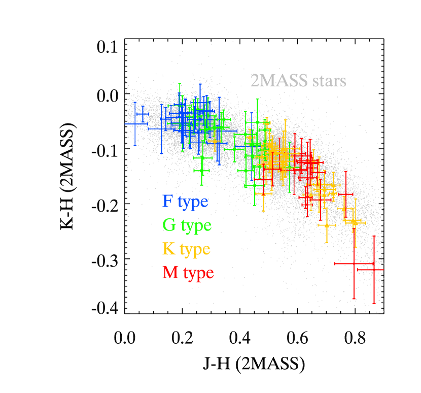
Figure 6: Color-color diagram for all identified stars. The J-H and K-H color information is from 2MASS, and the type information is from the IRTF fit. The background gray dots indicate stars drawn from the 2MASS catalog of each CIBER field. The colors represent different stellar types. The scatter of types over the J-H color can be explained either by the noncontinuous IRTF library or by uncertainties in spectral subclass.

A color-color diagram for the star sample is shown in Figure 6. Although the color-color diagram does not allow us to clearly discriminate between spectral types, qualitatively earlier-type stars are located in the bluer region, while later-type stars are located in the redder region, consistent with expectations. LRS stars well follow the color-color distributions of typical 2MASS stars in LRS fields, as indicated by the gray dots.

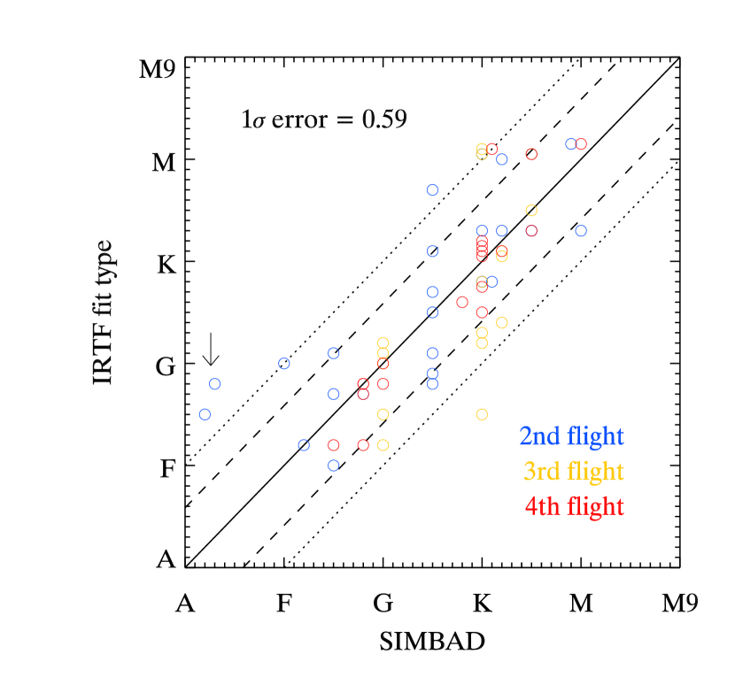
Figure 7: Type comparison determined from the IRTF fit and the literature for 63 stars whose types are already known. The dashed and dotted lines represent the 1$\sigma$ error and $\pm$1 spectral type, respectively. The colors represent the different flights’ data. Two A-type stars, indicated by an arrow, are fitted to F-type stars. Fit types based on the Pickles library also give the same results.

To estimate the error in our spectral type determination, we compare our identifications with the SIMBAD database (Wenger et al., 2000), where 63 of the 105 stars have prior spectral type determinations. Figure 7 shows the spectral types determined from the IRTF fit versus those from the SIMBAD database. The 1$\sigma$ error of type difference is estimated to be 0.59 spectral subtypes, which is comparable with those in other published works (Gliese, 1971; Jaschek & Jaschek, 1973; Jaschek, M., 1978; Roeser, 1988; Houk et al., 1999). The error can be explained with two factors: (i) the low spectral resolution of the LRS and (ii) the SED template libraries, which do not represent all star types.

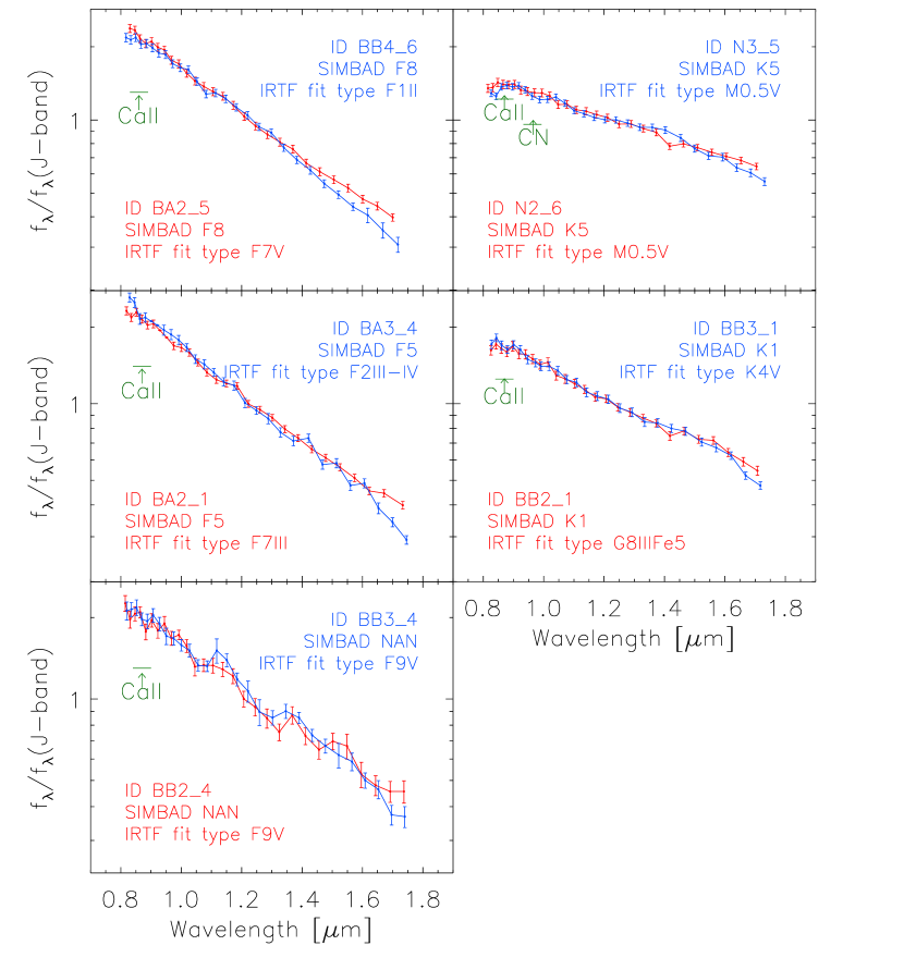
Figure 8: Five stars are serendipitously observed in two independent flights. Each panel shows two spectra extracted from each flight. Top left panel: 2nd flight (BA2_5), 4th flight (BB4_6). Top right panel: 2nd flight (N2_6), 3rd flight (N3_5). Middle left panel: 2nd flight (BA2_1), 3rd flight (BA3_4). Middle right panel: 2nd flight (BB2_1), 3rd flight (BB3_1). Bottom left panel: 2nd flight (BB2_4), 3rd flight (BB3_4). The large discrepancies arise from calibration error above 1.6 $\micron$ but show consistency of in-flight calibration below 1.6 $\micron$.

Five stars are observed twice in different flights (BA2_5 and BB4_6, N2_6 and N3_5, BA2_1 and BA3_4, BB2_1 and BB3_1, and BB2_4 and BB3_4; see Figure 8), enabling us to investigate the interflight stability of the spectra. For BA2_5 and BB4_6, the spectral type is known to be F8, while our procedure yields F7V and F1II from the second- and fourth-flight data, respectively. For N2_6 and N3_5, the known type is K5 while we determine M0.5V for both flights. For BA2_1 and BA3_4, the known type is F5 while we determine F7III and F2III-IV in the second and third flights. For BB2_1 and BB3_1, the fitted types are G8IIIFe5 and K4V for a K1 type star, and the type of BB2_4 and BB3_4 are not known but are fitted to F9V for both flights. The determined spectra are consistent within an acceptable error window, though the longer-wavelength data exhibit large differences, which can be attributed to calibration error. We present the spectra of each star from both flights in Table 3. This duplication results in our reporting of 110 spectra in the catalog, even through only 105 individual stars are observed.

5 Discussion

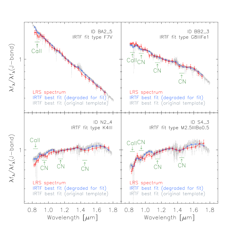
Figure 9: Representative examples of LRS spectra from this work. The color code is the same as that in Figure 5. F, G, K, and M stellar types are shown in each panel. Compared to other types, a typical F-type spectrum (top left panel) does not show any obvious absorption features across the wavelength range. We identified several features in our LRS spectra that correspond to typical absorption lines in the near-IR (i.e., CaII with bandhead at 0.85 $\micron$, CN with bandhead at 0.95, 1.15, and 1.5 $\micron$). The strongest feature in the F-type stars (top left) is the CaII triplet line, indicated with an arrow at 0.85 $\micron$. From types later than G (top right), CN bands appear with bandheads at 1.1, 0.91, 0.94, and 1.4$\micron$. We also identified M-type stars, as indicated in the bottom right panel. Since M-type stars have dominant molecular bands in their spectra, the identified lines are blended with other strong molecular bands, such as TiO (bandhead at 0.82$\micron$), ZrO (bandhead at 0.93$\micron$), FeH (bandhead at 0.99$\micron$), and H₂O (bandhead at 1.4$\micron$). The strength of each line depends on the spectral type.

We determined the spectral type of 105 stars as well as the associated typing error (0.59 spectral subtypes) assessed by comparing the type against a set of 63 previously determined spectral types. Representative examples of the measured spectra for different spectral types are shown in Figure 9. Molecular absorption lines are evident in these spectra, including the CaII triplet and various CN bands.

Since we observed stars above the earth’s atmosphere, observations of the H₂O molecular band are possible. However, they are not able to distinguish between CN and H₂O at 1.4 $\micron$ since both have the same bandhead and appear in late-type stars (Wing & Spinrad, 1970). For example, the spectral features of M2-M4 (super)giant stars observed by Stratoscope II, previously identified as CN, were identified as H₂O (Tsuji et al., 2000). Several subsequent observations show clear evidence that water features exist even in K type stars, requiring modifications of present stellar photosphere models (Tsuji et al., 2000).

In our spectral catalog, most K and M type stars exhibit a broad absorption band around 1.4 $\micron$. Although it is not possible to identify specific molecular bands with our data, we cannot exclude the presence of H₂O in the spectra of these stars. Future mid-IR measurements at $6.3\micron$ would help disentangle the source of the spectral features by removing the spectral degeneracies between CN and H₂O (Tsuji et al., 2001).

As these spectra are free from telluric contamination and the LRS is calibrated against absolute irradiance standards (Arai et al., 2015), in principle these measurements could be used as near-IR spectral standards. However, our lack of knowledge of the instrument response function (IRF) on the spectral plane complicates the use of these measurements for the absolute photometric calibration of stars. Specifically, the LRS’s IRF depends on the end-to-end optical properties of the instrument. Because we use a slit mask at the focus of an optical coupler (Tsumura et al., 2013), the full IRF knowledge of the focusing element of the optical coupler is difficult to disentangle from other effects. As a result, we would need to know the precise IRF to assign an absolute error estimate to an absolute calibration of the star images. This response function was not characterized during ground testing.

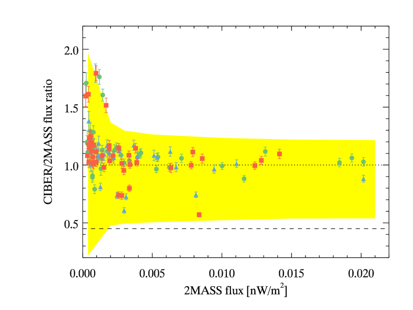
Figure 10: Flux ratios of all LRS stars to the matched 2MASS stars in the J-band. Each color represents the stars observed from each flight. Since the LRS flux is apodized by the slit mask, an aperture correction has been made to yield ratio unity in the ideal case (dotted line). The averaged original flux ratio is drawn as a dashed line, and its reciprocal is used for aperture correction. The color-shaded area shows the range of relation we expect from an instrument simulation, representing the upper and lower bounds of the absolute calibrations of the LRS.

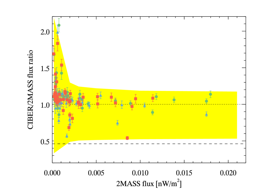
Figure 11: Same as Figure 10 but for the H-band.

Nevertheless, we consider it instructive to check the validity of photometric results whether or not the estimated magnitudes of the LRS stars are reasonable compared to previous measurements. We perform an empirical simulation as follows. For each LRS star, we generate a point source image with the flux of the 2MASS counterpart convolved to the LRS PSF. Instrumental noise and source confusion from faint stars ($J>13$) based on the 2MASS stars around a target star are also added. We measure the photometric flux of the simulated star image in the same way as for the LRS stars as described in this paper. An aperture correction is applied to the LRS stars, since stars that are clipped by the slit mask will appear to have a reduced flux measurement. Figures 10 and 11 show the ratios of the band-synthesized flux of each LRS star to the flux of the corresponding 2MASS star with statistical errors. The range explained by our simulations is illustrated as a color-shaded area. The LRS stars fall within the expected flux range. Also, the flux ratios of the stars between flights well agree, validating the stability of the photometric calibrations for the three CIBER flights. The large scatter at faint stars is caused by background noise, including adjacent faint stars and the instrument. The statistical J- and H-band flux errors are 3.89 % and 4.51 %, with systematic errors of 2.98 % and 3.82 %. We conclude that the achievable uncertainties on the absolute photometric amplitudes of these spectra are not competitive with other measurements (e.g. the existing 2MASS J and H-band flux errors are 1.57 % and 2.36 %, respectively).

The slit mask apodization correction ultimately limits the accuracy of our absolute calibration measurement and can lead to subtle biases. However, by connecting them with precise spectral measurements, we can improve the accuracy of LRS stellar spectra. The European Space Agency’s Gaia (Perryman et al., 2001; Jordi et al., 2010) mission is a scanning all-sky survey that uses a blue photometer (0.33$\micron$ $<$ $\lambda$ $<$ 0.68$\micron$) and a red (0.64$\micron$ $<$ $\lambda$ $<$ 1.05$\micron$) one to cover 0.33$\micron$ to 1.05$\micron$ with spectral resolution similar to that of the LRS. Because the Gaia photometers spectrally overlap with the LRS, we expect to eventually be able to unambiguously correct for the slit mask apodization and achieve an absolute flux calibration with less than 2 % accuracy over the full range $0.4\leq\lambda\leq 1.6\,\mu$m for our 105 stars.

In addition, the data reduction procedure described here may be a useful guide for the Gaia analysis. Since Gaia uses a prism-based photometer source detection, the data will show a nonlinear spatial variation of constant-wavelength bands and flux losses by a finite window size, as in our measurements. The background estimation will also require careful treatment with precise estimation of the end-to-end Gaia PSF.

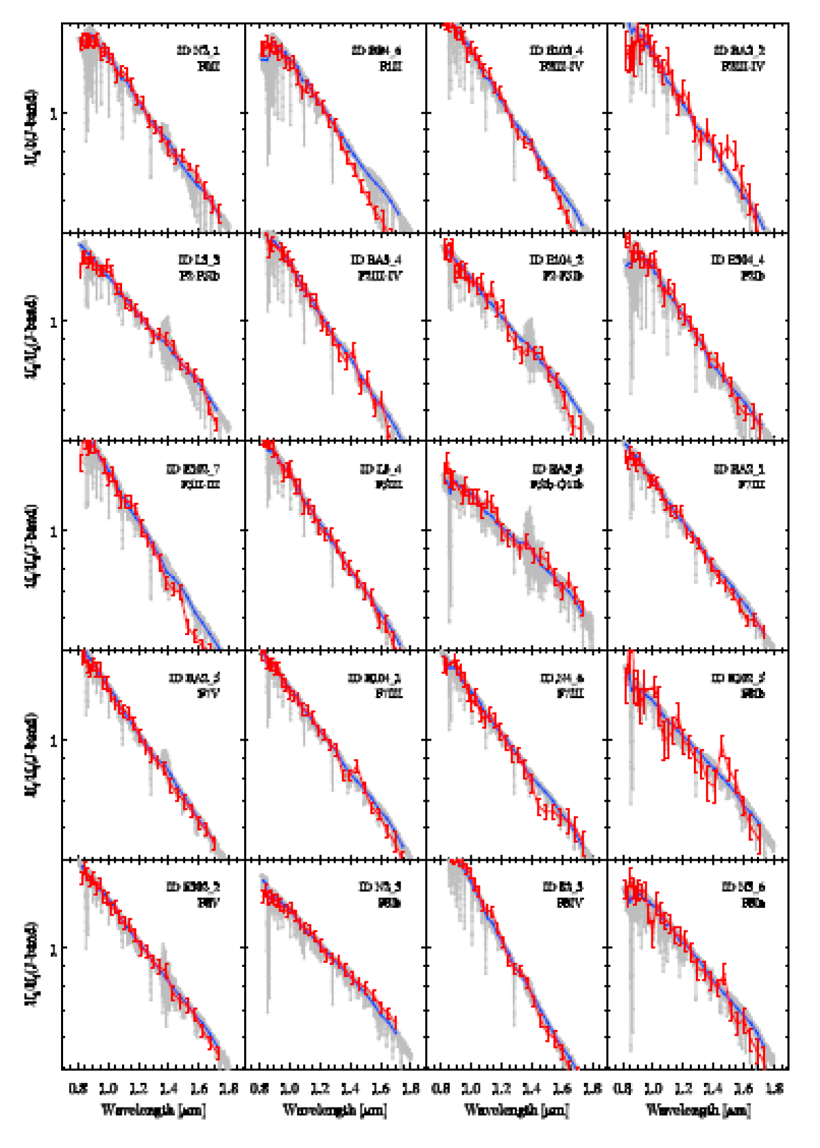
Figure 5: LRS spectra of stars identified in this survey. The blue curve represents the IRTF template degraded to fit the observed LRS spectrum, indicated by a red curve. All spectra are normalized at the J-band. The original template (gray color) is superimposed for comparison. The LRS ID and best-fit IRTF type are indicated on the upper right at each panel. (b)-(f) LRS spectra identified in this work. The color code is the same as that in Figure 5.

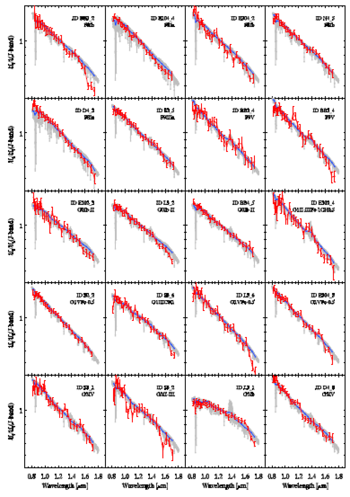
Figure 5 (Contnued): Continued.

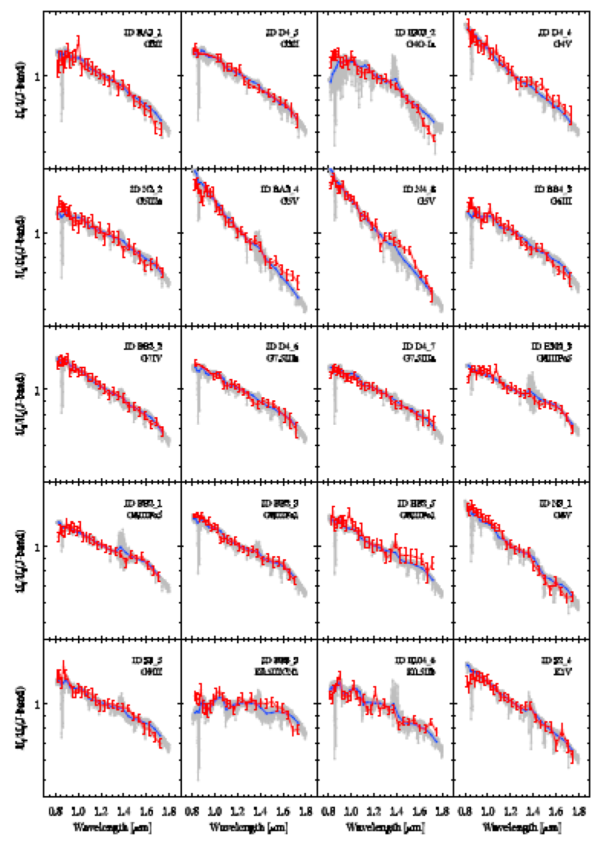
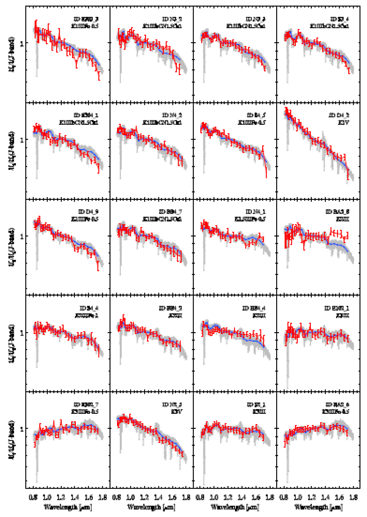
Figure 5 (Contnued): Continued.

Figure 5 (Contnued): Continued.

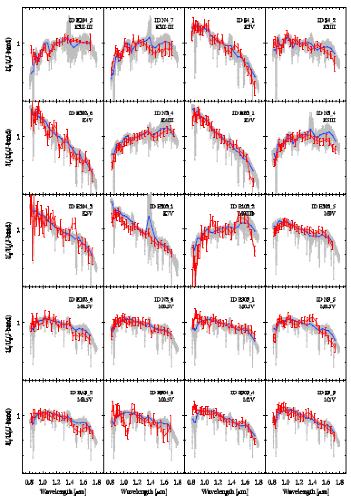
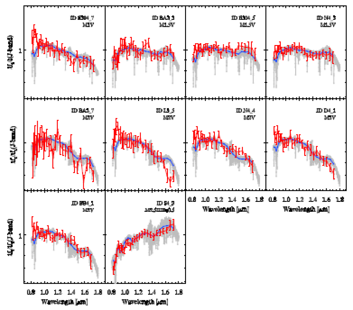
Figure 5 (Contnued): Continued.

Figure 5 (Contnued): Continued.

Table 1: Rocket-Commanded Coordinates for the observed field. Arabic numbers after the Hyphen for the Elat fields indicate the flight number

Field	R.A.	Decl.
Elat10-2	15:07:60.0	-2:00:00
Elat30-2	14:44:00	20:00:00
Elat30-3	15:48:00	9:30:00
Elat10-4	12:44:00	8:00:00
Elat30-4	12:52:00	27:00:00
NEP	18:00:00	66:20:23.987
SWIRE	16:11:00	55:00:00
BootesA	14:33:54.719	34:53:2.396
BootesB	14:29:17.761	34:53:2.396
Lockman	10:45:12.0	58:00:00
DGL	16:47:60.0	69:00:00

Table 2: Number of stars rejected at each criterion

Flight	Total Candidates	Crit.(i)	Crit.(ii)	Crit.(iii)	Crit.(iv)	Total in Final Catalog
2nd flight	198	15	43	8	145	38
3rd flight	177	14	41	6	127	30
4th flight	171	23	43	5	117	42

Table 3: Star catalog

Flight	Field	ID	Name	R.A.	Decl.	LRS J	LRS H	2MASS J	2MASS H	SIMBAD type	Best-fit IRTF Type	$\chi^{2}$	Note
	Elat10	E102_1	TYC5000-614-1	15:06:50.134	-00:02:47.746	9.020	8.283	8.283	7.608	K2	K3III	0.720	…
	Elat10	E102_2	…	14:59:05.568	-01:08:23.294	9.095	8.279	8.350	7.484	…	M0IIIb	4.582	…
	Elat10	E102_3	HD131553	14:54:20.898	-01:52:19.938	9.576	9.241	8.673	8.472	F0V	G0Ib-II	0.522	…
	Elat10	E102_4	HD134456	15:09:58.320	-00:52:47.269	7.872	7.754	6.982	6.854	F2III	F2III-IV	0.076	…
	Elat10	E102_5	TYC5001-847-1	15:14:43.328	-01:31:43.763	9.940	9.633	9.226	8.898	…	F8Ib	0.416	…
	Elat10	E102_6	BD-01-3038	15:14:15.481	-01:37:09.268	8.273	7.633	7.477	6.862	K0	M0.5V	0.462	…
	Elat10	E102_7	HD133213	15:03:28.468	-03:10:05.732	8.802	8.751	8.066	8.030	A2III	F5II-III	0.086	…
	Elat30	E302_1	BD+22-2745	14:46:03.405	22:04:37.528	8.065	7.499	7.158	6.664	G5	K7V	0.304	…
	Elat30	E302_2	HD127666	14:32:02.149	22:04:47.600	8.645	8.396	7.866	7.676	G5	F8V	0.045	…
	Elat30	E302_3	HD131132	14:51:16.019	18:38:59.284	6.648	6.111	5.803	5.334	K0	G8IIIFe5	0.260	…
	Elat30	E302_4	BD+19-2867	14:49:56.793	18:37:29.741	10.875	10.668	10.195	9.928	G5	G1II-IIIFe-1CH0.5	0.705	…
	Elat30	E302_5	BD+19-2857	14:45:32.922	18:40:20.255	7.342	6.643	6.466	5.815	K2	M0V	0.234	…
	Elat30	E302_6	TYC1481-620-1	14:46:48.921	17:30:12.359	10.208	9.644	9.620	9.138	…	K4V	0.551	…
	Elat30	E302_7	BD+18-2928	14:45:45.544	17:30:17.950	6.555	5.752	5.752	5.050	M0	K3IIIFe-0.5	1.488	…
2nd	NEP	N2_1	BD+68-954	17:43:43.944	68:24:26.593	10.067	9.742	9.394	9.168	F5	F0II	0.064	…
	NEP	N2_2	…	17:38:56.867	66:22:12.587	10.726	10.216	10.440	9.937	…	G5IIIa	0.240	…
	NEP	N2_3	BD+67-1039A	17:52:45.953	67:00:12.935	8.925	8.587	8.571	8.130	…	F8Ib	0.045	…
	NEP	N2_4	TYC4208-116-1	17:49:23.407	65:28:22.606	7.646	6.837	6.840	6.047	…	K4III	0.807	…
	NEP	N2_5	BD+67-1067	18:20:50.229	67:55:01.776	8.199	7.694	7.430	6.939	K0	K3V	0.119	…
	NEP	N2_6	HD166779	18:07:35.504	63:54:12.298	6.544	5.874	5.706	5.078	K5	M0.5V	0.221	…
	SWIRE	S2_1	HD144245	16:01:58.920	56:36:03.496	6.921	6.238	6.173	5.505	K5	K3III	0.201	…
	SWIRE	S2_2	HD144082	16:01:09.819	56:26:23.172	7.929	7.644	7.135	6.944	F5	G1VFe-0.5	0.051	…
	SWIRE	S2_3	HD147733	16:20:51.242	54:23:10.320	8.172	8.125	7.414	7.351	A3	F8IV	0.059	…
	SWIRE	S2_4	HD234317	16:32:27.630	54:20:14.320	8.713	8.283	7.999	7.564	G5	K1V	0.081	…
	SWIRE	S2_5	HD146736	16:15:15.896	52:01:48.338	8.929	8.618	8.140	7.884	G5	F9IIIa	0.060	…
	BootesA	BA2_1	HD126878	14:27:13.534	34:43:19.996	8.631	8.385	7.783	7.640	F5	F7III	0.046	…
	BootesA	BA2_2	TYC2557-719-1	14:41:46.727	33:34:23.452	10.800	10.557	10.045	9.783	…	F2III-IV	0.331	…
	BootesA	BA2_3	TYC2556-652-1	14:33:46.073	33:34:53.886	10.341	9.620	9.352	8.717	K9V	M1.5V	1.125	high-proper-motion
	BootesA	BA2_4	BD+34-2527	14:25:57.827	33:34:32.984	9.846	9.426	9.250	8.973	G5III	G5V	0.120	…
	BootesA	BA2_5	HD126210	14:23:24.060	33:34:19.099	8.480	8.274	7.653	7.492	F8	F7V	0.039	…
	BootesA	BA2_6	BD+34-2522	14:21:54.490	33:34:35.580	7.311	6.514	6.307	5.545	K5	K3IIIFe-0.5	0.584	…
	BootesA	BA2_7	…	14:41:50.085	32:24:33.790	10.848	10.330	10.178	9.587	…	M2V	1.521	…
	BootesA	BA2_8	TYC2553-127-1	14:29:10.917	32:27:40.871	10.252	9.490	9.130	8.483	…	K2III	1.255	…
	BootesB	BB2_1	TYC2560-1157-1	14:38:39.909	35:31:13.224	9.347	8.799	8.611	8.100	K1	G8IIIFe5	0.143	…
	BootesB	BB2_2	BD+36-2489	14:24:52.634	35:32:12.714	9.026	8.530	8.773	8.484	G5	G7IV	0.107	…
	BootesB	BB2_3	BD+32-2490	14:34:03.366	32:06:02.588	9.640	9.089	8.835	8.414	K0	G8IIIFe1	0.127	…
	BootesB	BB2_4	BD+31-2630	14:33:01.264	30:56:33.554	10.240	9.793	9.504	9.246	…	F9V	0.336	…
	BootesB	BB2_5	TYC2553-961-1	14:24:21.497	30:58:03.684	10.323	9.713	9.351	8.864	…	G8IIIFe1	0.580	…
	Elat30	E303_1	BD+11-2874	15:52:08.230	10:52:28.103	7.882	7.169	6.692	6.012	K5V	M0.5V	0.330	spectroscopic binary
	Elat30	E303_2	HD141631	15:49:47.057	10:48:24.520	8.251	7.922	7.555	7.096	K2	G4O-Ia	0.206	…
	Elat30	E303_3	TYC947-300-1	15:50:53.577	09:41:15.828	10.379	9.841	9.861	9.310	…	K1IIIFe-0.5	0.595	…
	Elat30	E303_4	HD141531	15:49:16.496	09:36:42.408	7.718	7.052	6.971	6.337	K	M1V	0.089	…
	NEP	N3_1	HD164781	17:57:03.647	68:49:19.744	8.948	8.601	7.733	7.423	K0	G8V	0.076	…
	NEP	N3_2	TYC4428-1122-1	17:54:46.231	68:06:42.016	9.753	9.250	9.009	8.353	…	K1IIIbCN1.5Ca1	0.629	…
	NEP	N3_3	BD+67-1050	18:06:45.898	67:50:40.686	8.273	7.722	7.485	6.976	K2	K1IIIbCN1.5Ca1	0.134	…
	NEP	N3_4	BD+65-1248	18:12:21.398	65:36:17.381	7.214	6.492	6.359	5.635	K5	K5III	0.919	…
	NEP	N3_5	HD166779	18:07:35.504	63:54:12.298	6.711	6.077	5.706	5.078	K5	M0.5V	0.455	…
	NEP	N3_6	TYC4226-812-1	18:25:26.020	66:00:38.783	9.655	9.417	8.924	8.714	…	F8Ia	0.293	…
	SWIRE	S3_1	BD+55-1802	16:01:45.359	54:48:40.882	10.325	10.033	9.570	9.330	G0	G2IV	0.392	…
	SWIRE	S3_2	TYC3870-1085-1	15:54:21.929	53:36:47.786	10.417	10.198	9.554	9.300	…	G2II-III	0.871	…
3rd	SWIRE	S3_3	TYC3870-366-1	15:53:29.099	53:28:36.008	8.669	8.062	7.928	7.281	…	M1V	0.285	…
	SWIRE	S3_4	TYC3877-704-1	16:10:22.667	54:28:38.784	9.017	8.472	8.258	7.715	…	K1IIIbCN1.5Ca1	0.239	…
	SWIRE	S3_5	TYC3877-1592-1	16:01:43.031	53:06:25.855	10.233	9.746	9.566	9.077	…	G9III	0.136	…
	SWIRE	S3_6	TYC3878-216-1	16:25:31.829	53:25:25.453	9.065	8.709	8.364	8.020	…	G1IIICH1	0.214	…
	Lockman	L3_1	V*DM-UMa	10:55:43.521	60:28:09.613	7.975	7.476	7.194	6.621	K0III	G2Ib	0.233	…
	Lockman	L3_2	HD94880	10:58:21.518	59:16:53.422	7.787	7.482	6.900	6.629	G0	G0Ib-II	0.115	…
	Lockman	L3_3	HD92320	10:40:56.905	59:20:33.065	7.947	7.662	7.148	6.852	G0	F2-F5Ib	0.109	high-proper-motion
	Lockman	L3_4	HD237955	10:57:44.114	58:10:01.103	9.799	9.619	8.705	8.508	G0	F5III	0.038	…
	Lockman	L3_5	TYC3827-847-1	11:01:59.570	56:58:11.510	9.498	9.094	8.816	8.279	…	M2V	0.479	…
	Lockman	L3_6	HD237961	11:00:12.007	56:59:49.481	9.267	9.049	8.495	8.271	G0	G1VFe-0.5	0.304	…
	BootesA	BA3_1	BD+362491	14:26:05.241	35:50:00.776	8.897	8.498	8.095	7.676	K0	G3II	0.515	…
	BootesA	BA3_2	HD128368	14:35:32.053	34:41:11.540	7.436	6.789	6.530	5.942	K0	M0.5V	0.215	…
	BootesA	BA3_3	BD+35-2576	14:32:31.567	34:42:09.493	9.291	8.834	9.058	8.737	K0	F5Ib-G1Ib	0.143	…
	BootesA	BA3_4	HD126878	14:27:13.534	34:43:19.996	9.190	9.091	7.783	7.640	F5	F2III-IV	0.060	…
	BootesB	BB3_1	TYC2560-1157-1	14:38:39.909	35:31:13.224	9.416	8.918	8.611	8.100	K1	K4V	0.124	…
	BootesB	BB3_2	BD+32-2503	14:41:07.455	32:04:45.095	9.628	9.449	8.853	8.624	…	F8Ib	0.198	…
	BootesB	BB3_3	BD+32-2456	14:18:52.718	32:06:31.003	9.191	8.531	7.992	7.444	K2III	K0.5IIICN1	0.534	…
	BootesB	BB3_4	BD+31-2630	14:33:01.264	30:56:33.554	10.170	9.940	9.504	9.246	…	F9V	0.438	…
	Elat10	E104_1	HD111645	12:50:42.449	08:52:30.238	8.908	8.691	8.124	7.920	F8	F7III	0.041	…
	Elat10	E104_2	BD+11-2491	12:46:07.870	11:09:25.744	10.229	9.992	9.486	9.201	F8	F2-F5Ib	0.162	…
	Elat10	E104_3	…	12:41:28.720	10:52:57.907	10.959	10.368	10.599	10.096	…	K5V	0.702	…
	Elat10	E104_4	HD110777	12:44:20.102	06:51:16.916	8.442	8.212	7.663	7.418	G0	F8Ia	0.148	…
	Elat10	E104_5	BD+10-2440	12:33:51.920	09:31:54.156	8.139	7.372	6.662	5.860	…	K3II-III	1.012	…
	Elat10	E104_6	HD109824	12:37:48.044	04:59:07.195	6.860	6.296	6.092	5.542	K0	K0.5IIb	0.570	…
	Elat30	E304_1	…	13:02:54.144	26:23:27.762	8.966	8.441	8.267	7.756	…	K1IIIbCN1.5Ca1	0.478	…
	Elat30	E304_2	BD+27-2207	13:02:50.671	26:50:00.402	10.924	10.630	10.141	9.899	F8	F8Ib	0.262	…
	Elat30	E304_3	TYC1995-264-1	13:02:50.439	27:29:22.283	10.212	10.004	9.586	9.251	…	G1VFe-0.5	0.121	…
	Elat30	E304_4	BD+27-2197	12:57:45.577	27:01:51.600	10.562	10.374	9.873	9.672	F5	F2Ib	0.098	…
	Elat30	E304_5	TYC1995-1123-1	12:57:25.736	28:18:25.992	9.837	9.006	8.997	8.229	…	M1.5V	0.608	…
	Elat30	E304_6	LP322-154	12:57:04.818	29:30:36.860	10.454	9.808	9.740	9.096	K5V	M0.5V	1.460	high-proper-motion
	Elat30	E304_7	TYC2532-820-1	12:56:45.236	30:44:22.556	10.678	10.006	9.838	9.324	K1V	M1V	0.344	…
	NEP	N4_1	BD+68-951	17:38:51.760	68:13:16.536	9.137	8.449	7.942	7.438	K0	K1.5IIIFe-0.5	0.273	multiple-star
	NEP	N4_2	HD161500	17:41:10.318	65:13:10.301	7.442	6.860	6.633	6.119	K2	K1IIIbCN1.5Ca1	0.312	…
	NEP	N4_3	G227-20	17:52:11.850	64:46:08.720	9.077	8.391	8.249	7.615	M0.5V	M1.5V	0.449	high-proper-motion
4th	NEP	N4_4	TYC4208-1599-1	17:52:05.421	64:37:15.827	10.278	9.725	9.929	9.259	…	M2V	0.486	…
	NEP	N4_5	BD+64-1227A	17:52:17.178	64:14:16.411	8.816	8.500	8.400	8.125	…	F8Ib	0.046	…
	NEP	N4_6	TYC4213-161-1	18:03:24.923	67:12:41.681	10.171	9.868	9.327	9.115	…	F7III	0.109	…
	NEP	N4_7	BD+66-1074	18:03:15.008	66:20:29.069	7.609	6.866	6.739	6.046	K5	K3II-III	1.262	…
	NEP	N4_8	HD170592	18:25:24.759	65:45:34.470	7.474	7.143	6.722	6.409	K0	G5V	0.148	…
	SWIRE	S4_1	TYC3870-1026-1	15:55:16.319	54:45:12.510	10.127	9.564	9.332	8.829	…	K3V	0.261	…
	SWIRE	S4_2	TYC3496-1361-1	15:56:04.610	52:13:29.543	8.240	7.566	7.519	6.825	…	K3III	0.421	…
	SWIRE	S4_3	TYC3880-1133-1	16:03:15.627	56:02:35.210	8.711	7.821	7.791	6.995	…	M2.5IIIBa0.5	2.347	…
	SWIRE	S4_4	TYC3877-484-1	16:03:12.065	54:44:27.658	9.047	8.361	7.846	7.288	…	K2IIIFe-1	0.147	…
	SWIRE	S4_5	HD234308	16:26:05.554	52:18:08.266	8.652	8.101	7.932	7.407	K0	K1IIIFe-0.5	0.237	…
	DGL	D4_1	TYC4419-1623-1	16:14:22.875	69:55:54.455	10.093	9.624	9.419	8.810	…	M2V	0.373	…
	DGL	D4_2	TYC4419-1631-1	16:18:10.929	69:16:36.761	9.923	9.466	9.229	8.916	…	K1V	0.124	…
	DGL	D4_3	BD+67-943	16:29:52.210	66:47:45.154	9.390	9.120	8.606	8.417	F8	F8Ia	0.110	…
	DGL	D4_4	TYC4196-2280-1	16:34:34.354	65:36:05.818	10.424	9.946	9.783	9.339	…	G4V	0.232	…
	DGL	D4_5	HD151286	16:40:37.776	70:34:14.772	7.110	6.668	6.237	5.794	…	G3II	0.070	…
	DGL	D4_6	BD+69-873	16:47:31.365	68:51:02.603	8.338	7.820	7.495	7.010	K0	G7.5IIIa	0.111	…
	DGL	D4_7	HD154273	16:58:40.137	69:38:05.431	7.022	6.508	6.197	5.746	K0	G7.5IIIa	0.106	…
	DGL	D4_8	TYC4424-1380-1	17:08:33.058	71:00:28.044	9.242	8.911	9.008	8.727	…	G2IV	0.109	…
	DGL	D4_9	TYC4421-2278-1	17:16:54.688	67:38:26.279	8.993	8.460	8.269	7.792	…	K1IIIFe-0.5	0.174	…
	BootesB	BB4_1	TYC2557-870-1	14:40:08.540	34:40:29.669	10.107	9.545	9.249	8.768	…	M2V	0.331	…
	BootesB	BB4_2	HD128094	14:34:10.846	30:59:10.356	7.857	7.240	6.963	6.405	K0	K2III	0.226	…
	BootesB	BB4_3	TYC2559-388-1	14:34:47.808	35:34:09.419	9.761	9.346	9.011	8.550	G8V	G6III	0.184	…
4th	BootesB	BB4_4	TYC2553-947-1	14:28:52.868	31:30:30.316	8.505	7.763	7.642	6.917	…	K2III	0.170	…
	BootesB	BB4_5	V*KT-Boo	14:29:02.513	33:50:38.929	8.699	8.271	7.846	7.465	G	G0Ib-II	0.074	…
	BootesB	BB4_6	HD126210	14:23:24.060	33:34:19.099	8.764	8.749	7.653	7.492	F8	F1II	0.194	…
	BootesB	BB4_7	TYC2549-413-1	14:23:23.452	34:33:24.854	9.399	8.885	8.510	7.947	…	K1IIIbCN1.5Ca1	0.269	…

References

- Arai et al. (2015) Arai, T., Matsuura, S., Bock, J., et al. 2015, ApJ, 806, 69
- Bock et al. (2006) Bock, J., Battle, J., Cooray, A., et al. 2006, New A Rev., 50, 215
- Bock et al. (2013) Bock, J., Sullivan, I., Arai, T., et al. 2013, ApJS, 207, 32
- Bohlin & Gilliland (2004) Bohlin, R. C., & Gilliland, R. L., 2004, AJ, 127, 3508 (BG)
- Cohen et al. (2003) Cohen, M., Wheaton, Wm. A., & Megeath, S. T. 2003, AJ, 126, 1090
- Cushing (2005) Cushing, M. C. 2005, ApJ, 623, 1115
- Fischer et al. (1998) Fisher, J., Baumback, M. M., Bowles, J. H., Grossmann, J. M., & Antoniades, J. A. 1998, Proc SPIE, 3438, 23
- Garnett & Forrest (1993) Garnett, J., D.P., & Forrest, W.J., 1993, SPIE, 1946, 395G
- Gliese (1971) Gliese, W. 1971, Veroeffentlichungen des Astronomischen Rechen-Instituts Heidelberg, 24, 1
- Hauser & Dwek (2001) Hauser, M.G. & Dwek, E., 2001, ARA&A, 39, 249
- Houk et al. (1999) Houk, N., & Swift, C. 1999, University of Michigan Catalogue of Two-Dimensional Spectral Types for the HD Stars, Vol. 5 (Ann Arbor: Univ. Michigan)
- Jaschek, M. (1978) Jaschek, M. 1978, CDS Inf. Bull. 15, 121
- Jaschek & Jaschek (1973) Jaschek, C., & Jaschek, M. 1973, in IAU Symp. 50, Spectral Classification and Multicolour Photometry, ed. C. Fehrenbach & B. E. Westerlund (Dordrecht:Reidel), 43
- Jordi et al. (2010) Jordi, C., Gebran, M., Carrasco, J. M., et al. 2010, A&A, 523, A48
- Joyce et al. (1998) Joyce, R. R., Hinkle, K. H., Wallace, L., Dulick, M., & Lambert, D. L., 1998, AJ, 116, 2520
- Kessler et al. (1996) Kessler, M. F., Steinz, J. A., & Anderegg, M. E., et al. 1996, A&A, 315, L27
- Korngut et al. (2013) Korngut, P. M., Renbarger, T., Arai, T., et al. 2013, ApJS, 207, 34
- Lee et al. (2010) Lee, D. H., Kim, M. G., Tsumura, K., et al. 2010, Journal of Astronomy and Space Sciences, 27, 401
- Leinert et al. (1998) Leinert, Ch., Bowyer, S., Haikala, L. K., et al. 1998, A&AS, 127, 1L
- Madau & Pozzetti (2000) Madau, P. & Pozzetti, L., 2000, MNRAS, 312, L9-L15
- Matsumoto et al. (2005) Matsumoto, T., Matsuura, S., Murakami, H., et al. 2005, ApJ, 626, 31
- Matsuura et al. (1999) Matsuura, M., Yamamura, I., Murakami, H., Freund, M. M., & Tanaka, M. 1999, A&A, 348, 579
- Matsuura et al. 2016, ApJ, submitted (2016) Matsuura, S., Arai, T., Bock, J., et al. 2016, ApJ, submitted
- Meyer et al. (1998) Meyer, M. R., Edwards, S., Hinkle, K. H., & Strom, S. E., 1998, ApJ, 508, 397
- Murakami et al. (1996) Murakami, H., Freund, M. M., Ganga, K., et al. 1996, PASJ, 48, L41
- Peterson et al. (2008) Peterson, D. E., Megeath, S. T., Luhman, K. L., et al. 2008, ApJ, 685, 313
- Perryman et al. (2001) Perryman, M. A. C., de Boer, K. S., Gilmore, G., et al. 2001, A&A, 369, 339
- Pickles (1998) Pickles, A. J. 1998, PASP, 110, 863
- Rayner (2009) Rayner, J. T. 2009, ApJS, 185, 289
- Roeser (1988) Roeser, S. & Bastian, U., 1988, A&A, 74, 449
- Russell (1934) Russell, H. N. 1934, ApJ, 79, 317
- Schlegel (1998) Schlegel, D. J. 1998, ApJ, 500, 525
- Skrutskie et al. (2006) Skrutskie, M. F., Cutri, R. M., Stiening, R., et al. 2006, AJ, 131, 1163S
- Sorahana & Yamamura (2014) Sorahana, S., Yamamura, I. 2014, ApJ, 793, 47
- Tsumura et al. (2010) Tsumura, K., Battle, J., Bock, J., et al. 2010, ApJ, 719, 394
- Tsumura et al. (2013) Tsumura, K., Arai, T., Battle, J., et al. 2013, ApJS, 207, 33
- Tsuji et al. (1997) Tsuji, T., Ohnaka, K., Aoki, W., & Yamamura, I. 1997, A&A, 320, L1
- Tsuji et al. (2000) Tsuji, T. 2000, ApJ, 538, 801
- Tsuji et al. (2001) Tsuji, T. 2001, A&A, 376, L1
- Tsuji et al. (2015) Tsuji, T. 2015, PASJ, 67, 26T
- Wenger et al. (2000) Wenger, M., Ochsenbein, F., Egret, D., et al. 2000, A&AS, 143, 9
- Wing & Spinrad (1970) Wing, R. F., & Spinrad, H. 1970, ApJ, 159, 973
- Woolf et al. (1964) Woolf, N. J., Schwarzschild, M., & Rose, W. K. 1964, ApJ, 140, 833
- Yuan et al. (2013) Yuan, H. B., Liu, X. W., & Xiang, M. S. 2013, MNRAS, 430, 2188
- Zemcov et al. (2013) Zemcov, M., Arai, T., Battle, J., et al. 2013, ApJS, 207, 31