Fractality and degree correlations in scale-free networks

Abstract

Fractal scale-free networks are empirically known to exhibit disassortative degree mixing. It is, however, not obvious whether a negative degree correlation between nearest neighbor nodes makes a scale-free network fractal. Here we examine the possibility that disassortativity in complex networks is the origin of fractality. To this end, maximally disassortative (MD) networks are prepared by rewiring edges while keeping the degree sequence of an initial uncorrelated scale-free network that is guaranteed to become fractal by rewiring edges. Our results show that most of MD networks with different topologies are not fractal, which demonstrates that disassortativity does not cause the fractal property of networks. In addition, we suggest that fractality of scale-free networks requires a long-range repulsive correlation in similar degrees.

I INTRODUCTION

Networks describing complex systems in the real world are quite inhomogeneous and complicated Albert02 ; Dorogovtsev08 ; PasterSatorras15 . The number of edges from a node, namely degree, for example, is widely distributed in a network. In fact, many real-world complex networks have asymptotically power-law degree distributions, which is called the scale-free property Barabasi99 . In addition, the degrees of adjacent nodes via an edge are usually correlated. Such nearest neighbor degree correlations can be described by the joint probability $P(k,k^{\prime})$ of a randomly chosen edge connecting two nodes with degrees $k$ and $k^{\prime}$. It has been empirically known that nodes in social networks tend to be connected to nodes with similar degrees (assortative mixing) while technological or biological networks show the opposite tendency (disassortative mixing) Newman02 ; Newman03 . Network complexity is also characterized by the shortest path distance (number of edges along the shortest path) between nodes. From this point of view, most of real-world networks can be classified into two classes Kawasaki10 , namely, small-world networks Watts98 and fractal networks Song05 . In a small-world network, the shortest path distance averaged over all node pairs increases logarithmically (or more slowly) with the total number of nodes. In other words, the minimum number of subgraphs $N_{\text{B}}$ covering the entire network decreases exponentially (or faster) with the subgraph diameter, that is,

$$N_{\text{B}}(l_{\text{B}})\propto e^{-l_{\text{B}}/l_{0}},$$ (1)

where $l_{\text{B}}$ is the maximum distance between any nodes in the subgraph (subgraph diameter) and $l_{0}$ is a constant. It has been shown that many real-world networks possess the small-world property Albert02 ; Watts98 . For a fractal network, on the other hand, the number of covering subgraphs decreases with $l_{\text{B}}$ in a power-law manner, i.e.,

$$N_{\text{B}}(l_{\text{B}})\propto l_{\text{B}}^{-D},$$ (2)

where $D$ is the fractal dimension of the network. This relation has been observed also in a diverse range of networks from the World Wide Web to some kinds of cellular networks Kawasaki10 ; Song05 ; Gallos08 ; Gallos12 .

The origin of the fractal property in complex networks is still an open question Watanabe15 , though the mechanism of the small-world network formation has been found in the existence of short-cut edges. It has, however, been empirically demonstrated that real-world and synthetic fractal scale-free networks have disassortative degree correlations Yook05 ; Song06 ; Rozenfeld07 ; Kim09 . If the converse is also true, that is, disassortative mixing makes a scale-free network fractal, the origin of fractality would be found in the degree correlation. Disassortativity is a local property characterizing nearest neighbor degree correlations, while fractality is a consequence of long-range structural correlations. This fact seems to deny the above possibility. It is, however, known that if edges in a scale-free network are rewired to maximize or minimize the assortativity $r$ while keeping the degree sequence (and hence the degree distribution) then the maximally assortative or disassortative network becomes to possess a long-range correlation Menche10 . The assortativity $r$ is the Pearson’s correlation coefficient for degrees and defined by Newman02 ; Newman03

$$r=\frac{\displaystyle 2\sum_{(i,j)\in E}k_{i}k_{j}-\frac{1}{2M}\left[\sum_{(i,j)\in E}(k_{i}+k_{j})\right]^{2}}{\displaystyle\sum_{(i,j)\in E}(k_{i}^{2}+k_{j}^{2})-\frac{1}{2M}\left[\sum_{(i,j)\in E}(k_{i}+k_{j})\right]^{2}},$$ (3)

where $k_{i}$ is the degree of node $i$, $M$ is the total number of edges, and $E$ is the set of undirected edges in the network. A maximally assortative network has an onionlike structure consisting of communities of regular subgraphs Menche10 ; Schneider11 . Such a network displays a long-range structural correlation in which maximum degree nodes are distant from minimum degree ones. A maximally disassortative (MD) network also shows a community structure. In each community, all nodes with a specific low degree and higher degree nodes are connected alternately Menche10 . Thus, a minimum (or maximum) degree node is located far away from an intermediate degree node in the MD network, which implies a long-range correlation. Therefore, there is a possibility that even short-range disassortative degree mixing induces the long-range fractal correlation, as pointed out by Ref. Kim09 through the analysis of random critical branching trees. Furthermore, considering the entropic origin of disassortativity Johnson10 , we can discuss the formation mechanism of fractal scale-free networks in connection with a process maximizing the entropy.

In this paper, we examine the possibility that a negative degree correlation between nearest neighbor nodes makes a scale-free network fractal. To this end, we first prepare an uncorrelated scale-free network that is guaranteed to become fractal by rewiring edges. Then, this network is again rewired so that the nearest neighbor degree correlation becomes maximally negative. If the rewired MD network exhibits the fractal nature, one can conclude that fractality of scale-free networks is induced by disassortative degree mixing. Our results, however, show that disassortativity does not always make scale-free networks fractal. We also suggest that fractality seems to require a long-range repulsive correlation between similar degree nodes.

The rest of this paper is organized as follows. In Sec. II, we explain how to prepare the initial network $G_{\text{ini}}$ that can be fractal scale free by rewiring edges. The rewiring method to obtain MD networks is also described in this section. Our results on the fractal property of rewired disassortative networks are presented in Sec. III. A long-range degree correlation is also argued. Section IV is devoted to the summary and remarks.

II PREPARATION OF NETWORKS

We investigate the fractal property of MD networks formed by rewiring edges while keeping the degree distribution of a given initial uncorrelated scale-free network $G_{\text{ini}}$. In this section, we explain how to prepare the initial network $G_{\text{ini}}$ and how to rewire it so as to realize a MD network.

II.1 Preparing the initial network

The initial uncorrelated scale-free network $G_{\text{ini}}$ must be guaranteed to become fractal by rewiring edges. Such a network can be constructed by rewiring randomly edges of an original scale-free fractal network $G_{0}$. We adopt the $(u,v)$-flower with $2\leq u\leq v$ as the network $G_{0}$ Rozenfeld07 ; Dorogovtsev02 . In the $(u,v)$-flower model, we start with the cycle graph consisting of $w\equiv u+v$ nodes and edges [the first generation $(u,v)$-flower]. The $n$th generation $(u,v)$-flower $G_{n}^{(u,v)}$ is obtained by replacing each edge in $G_{n-1}^{(u,v)}$ by two parallel paths of $u$ and $v$ edges. The number of nodes $N$ and the number of edges $M$ in $G_{n}^{(u,v)}$ are given by

$$N = \frac{(w-2)w^{n}+w}{w-1},$$ (4)

$$M = w^{n}.$$ (5)

The degree of a node in this network falls into any of $2^{m}$ with $m=1,2,\dots,n$, and the number of nodes $N_{k_{m}}$ with the degree $k_{m}=2^{m}$ is given by

$$N_{k_{m}}=\begin{cases}(w-2)w^{n-m}&(1\leq m<n),\\ w&(m=n),\end{cases}$$ (6)

which specifies the degree sequence of the network. Thus, the degree distribution function $P(k)$ for $k\gg 1$ of $G_{n}^{(u,v)}$ with large $n$ is proportional to $k^{-\gamma}$, where

$$\gamma=1+\frac{\log w}{\log 2}.$$ (7)

The network with $u\geq 2$ exhibits fractality with the fractal dimension Rozenfeld07 ,

$$D_{\text{f}}=\frac{\log w}{\log u}.$$ (8)

The $4$th generation $(2,2)$-flower with $172$ nodes and $256$ edges is depicted in Fig. 1(a).

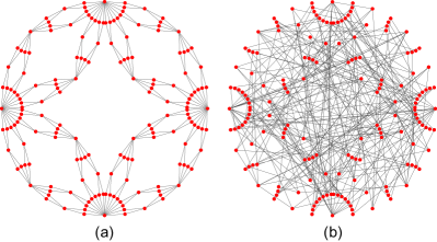
Figure 1: (a) The $4$th generation $(2,2)$-flower with $N=172$ nodes and $M=256$ edges. (b) A network formed by $5M$ operations of RR for the network shown by (a).

The initial network $G_{\text{ini}}$ is formed by rewiring randomly edges in the scale-free fractal $(u,v)$-flower as $G_{0}$. The random rewiring (RR) procedure is performed as follows:

(i) Choose randomly two edges $(i_{1},j_{1})$ and $(i_{2},j_{2})$ with four different end nodes, namely $(i_{1}-i_{2})(i_{1}-j_{2})(j_{1}-i_{2})(j_{1}-j_{2})\neq 0$.

(ii) Rewire these edges to $(i_{1},j_{2})$ and $(i_{2},j_{1})$, if this rewiring process does not make multiple edges.

(iii) Repeat (i) and (ii) enough times.

Since the above rewiring preserves the degree of each node, the degree sequence (and thus the degree distribution) of the network after RR’s does not change from the original one. If the number of repetition times is much larger than the number of edges $M$, the rewired network $G_{\text{ini}}$ possesses essentially the same statistical properties as the configuration model Bekessy72 ; Molloy95 ; Newman01 with the degree sequence specified by Eq. (6). Therefore, $G_{\text{ini}}$ has no degree correlations, as well as no structural correlations such as fractality. It should be, however, emphasized that the network $G_{\text{ini}}$ is guaranteed to become fractal by rewiring edges. As an example of $G_{\text{ini}}$, the network shown in Fig. 1(b) is formed by the RR procedure (i)-(iii) from the $(2,2)$-flower of Fig. 1(a).

II.2 Maximally disassortative network

In order to make MD networks $G_{\text{MD}}$ from an initial network $G_{\text{ini}}$, we first quantify the degree of assortative mixing in a network. The assortativity $r$ defined by Eq. (3) is widely used for this purpose. If $r$ is positive, the network is assortatively mixed on degrees of nodes, while a network with a negative $r$ shows disassortative mixing. It has been, however, pointed out that $r$ strongly depends on the network size and cannot be negative for infinitely large scale-free networks if the degree distribution decays asymptotically more slowly than $k^{-4}$ Menche10 ; Dorogovtsev10 ; Litvak13 ; Raschke10 . To overcome this problem, the Spearman’s rank correlation coefficient $\rho$ for degrees has been proposed for measuring assortative (or disassortative) mixing Litvak13 . This quantity is defined by

$$\rho=\frac{\displaystyle 2\sum_{(i,j)\in E}R_{k_{i}}R_{k_{j}}-\frac{1}{2M}\left[\sum_{(i,j)\in E}(R_{k_{i}}+R_{k_{j}})\right]^{2}}{\displaystyle\sum_{(i,j)\in E}(R_{k_{i}}^{2}+R_{k_{j}}^{2})-\frac{1}{2M}\left[\sum_{(i,j)\in E}(R_{k_{i}}+R_{k_{j}})\right]^{2}},$$ (9)

where $R_{k_{i}}$ is the rank of the degree of node $i$ and the meaning of the summation is the same as in Eq. (3). From the above definition, it is clear that $\rho$ is the Pearson’s correlation coefficient for degree ranks.

There are several ways to determine the rank $R_{k}$ if plural nodes in a network have the same degree. To avoid this problem, Litvak et al. Litvak13 resolve the rank degeneracy for the same degree nodes by using random numbers. This method, however, makes it difficult to calculate analytically $\rho$ even for a deterministic network such as the $(u,v)$-flower. An alternative way of ranking is to rank degrees of $2M$ end nodes in ascending order with assigning the average rank of degenerated degrees to them Zhang16 . In this case, the rank of an end node with degree $k$ is given by

$$R_{k}=\frac{kN_{k}+1}{2}+\sum_{k^{\prime}=0}^{k-1}k^{\prime}N_{k^{\prime}},$$ (10)

where $N_{k}=NP(k)$ is the number of nodes with degree $k$. Using this ranking, the Spearman’s rank correlation coefficient $\rho$ can be written as

$$\rho=\frac{\displaystyle 2\sum_{(i,j)\in E}R_{k_{i}}R_{k_{j}}-\frac{M}{2}(2M+1)^{2}}{\displaystyle\sum_{(i,j)\in E}(R_{k_{i}}^{2}+R_{k_{j}}^{2})-\frac{M}{2}(2M+1)^{2}},$$ (11)

where we use $\sum_{(i,j)\in E}(R_{k_{i}}+R_{k_{j}})=M(2M+1)$. It should be noted that topologies of networks with a specific degree sequence are reflected only in the first term $\sum_{(i,j)\in E}R_{k_{i}}R_{k_{j}}$ of the numerator. Since the rank $R_{k}$ one-to-one corresponds to $k$, analytical calculations of $\rho$ are possible for some deterministic networks. For example, $\rho$ for the $n$th generation $(u,v)$-flower $G_{n}^{(u,v)}$ with $u\geq 2$ and $n\geq 2$ is presented by (see the Appendix)

$$\rho_{n}^{(u,v)}=-\frac{z\left(z^{2}+z+1\right)}{1-z^{3(n-1)}},$$ (12)

where $z\equiv 2/(u+v)$ is less than or equal to $1/2$. For an infinitely large $(u,v)$-flower ($n\to\infty$), $\rho_{\infty}^{(u,v)}=-z(z^{2}+z+1)$ is negative for any $z$ as expected from Fig. 1(a), while the assortativity $r$ for $G_{\infty}^{(u,v)}$ with $z\geq 1/4$ becomes zero as shown in the Appendix.

We construct a MD network $G_{\text{MD}}$ by rewiring edges of $G_{\text{ini}}$ so as to minimize the Spearman’s rank correlation coefficient $\rho$. The actual rewiring procedure is as follows:

(i) Choose randomly two edges $(i_{1},j_{1})$ and $(i_{2},j_{2})$ with four different end nodes.

(ii) Rewire these edges to $(i_{1},j_{2})$ and $(i_{2},j_{1})$, if this rewiring does not make multiple edges and not increase the Spearman’s rank correlation coefficient $\rho$.

(iii) Repeat (i) and (ii) until $\rho$ cannot be decreased anymore by rewiring.

This disassortative rewiring (DR) also does not change the degree sequence. Therefore, $N_{k_{m}}$ of $G_{\text{MD}}$ is still given by Eq. (6). For some degree sequences, the rank correlation $\rho$ cannot reach its minimum value by the above DR scheme because of local minimum trap. In such a case, an optimization algorithm based on simulated annealing Donetti05 must be employed instead of the present DR. However, the above simple DR can minimize $\rho$ at least for the degree sequence specified by Eq. (6), as mentioned later.

III RESULTS

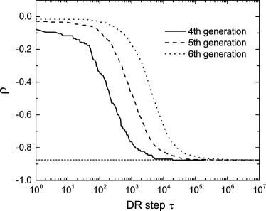
Figure 2: Rank correlation coefficient $\rho$ as a function of the number of DR steps $\tau$ starting from the initial networks ($G_{\text{ini}}$) formed by $5M$ operations of RR for the 4th (solid line), 5th (dashed line), and 6th (dotted line) generation $(2,2)$-flowers ($G_{0}$), where $M$ is the number of edges in the networks. The horizontal dotted line indicates the value of $\rho_{6}^{(2,2)}$.

Figure 2 shows how the rank correlation coefficient $\rho$ decreases with the DR step $\tau$ starting from $G_{\text{ini}}$. Initial networks $G_{\text{ini}}$ are formed by $5M$ operations of RR for $(2,2)$-flowers ($G_{0}$), where $M$ is the number of edges. Solid, dashed, and dotted curves in Fig. 2 represent the results for the 4th, 5th, and 6th generation $(2,2)$-flowers as $G_{0}$. The numbers of nodes $N$ and edges $M$ are $N=172$, $684$, and $2\,732$ and $M=256$, $1\,024$, and $4\,096$ for the 4th, 5th, and 6th generations, respectively. The initial values of $\rho$ at $\tau=0$ (i.e., $\rho$ for $G_{\text{ini}}$) are slightly negative even though $G_{\text{ini}}$ is randomly rewired enough times. This is because self-loops and multiple edges are not allowed in $G_{\text{ini}}$. Since the probability to have such edges by RR with allowing them decreases with the network size, $\rho$ for $G_{\text{ini}}$ becomes close to zero as the generation increases. The rank correlations $\rho$ monotonically decrease with the DR step, and reach negative constant values. These convergence values coincide with $\rho_{n}^{(2,2)}$ presented by Eq. (12), namely, $\rho_{4}^{(2,2)}=-0.8767$, $\rho_{5}^{(2,2)}=-0.8752$, and $\rho_{6}^{(2,2)}=-0.8750$ (indicated by the horizontal dotted line in Fig. 2). The rank correlations never diminish from these values even if repeating DR operation many times.

We can show that the above convergence value $\rho_{n}^{(u,v)}$ gives the minimum $\rho$ among networks with the degree sequence specified by Eq. (6), that is, networks with $\rho_{n}^{(u,v)}$ are nothing but MD networks. For simplicity, let us discuss the case of $\rho_{n}^{(2,2)}$ and define two sets, $S_{N_{k}}$ and $S_{\text{MD}}$, of networks derived from the $n$th generation $(2,2)$-flower. The set $S_{N_{k}}$ includes all networks with the degree sequence specified by Eq. (6), while $S_{\text{MD}}$ is a proper subset of $S_{N_{k}}$ in which every network is composed of edges connecting two nodes with the lowest degree $k_{1}=2$ and a higher degree $k_{m}=2^{m}$ with $m\geq 2$. Namely, a network in $S_{\text{MD}}$ has the joint probability $P(k,k^{\prime})$ for $k<k^{\prime}$ given by

$$P(k,k^{\prime})=\frac{1}{2M}\sum_{m=2}^{n}k_{m}N_{k_{m}}\delta_{k2}\delta_{k^{\prime}k_{m}},$$ (13)

where $N_{k_{m}}$ is presented by Eq. (6) and $M=w^{n}$ is the number of edges. The rank correlation coefficient $\rho$ takes a constant value for networks in $S_{\text{MD}}$ because $\rho$ of Eq. (11) is uniquely determined by $P(k,k^{\prime})$ and $R_{k}$ and the rank $R_{k}$ defined by Eq. (10) does not change for networks in $S_{N_{k}}$. Since the $(2,2)$-flower is an element of $S_{\text{MD}}$, this constant value is equal to $\rho_{n}^{(2,2)}$. If a network with the degree sequence $N_{k_{m}}$ given by Eq. (6) has a joint probability $P(k,k^{\prime})$ different from Eq. (13), the network possesses edges connecting lowest degree nodes to each other. In order to prove that $\rho$ of such a network is larger than $\rho_{n}^{(2,2)}$, let us consider a network $\tilde{G}$ formed by rewiring two edges $(i,j)$ and $(i^{\prime},j^{\prime})$ of a network $G\in S_{\text{MD}}$ to $(i,i^{\prime})$ and $(j,j^{\prime})$. Here, the degrees of these end nodes are $k_{i}=k_{i^{\prime}}=2$ and $k_{j}\geq k_{j^{\prime}}>2$. The network $\tilde{G}$ has the same $R_{k}$ as $G$ because $G,\tilde{G}\in S_{N_{k}}$, while $P(k,k^{\prime})$ for $\tilde{G}$ is slightly different from Eq. (13). For both $G$ and $\tilde{G}$, we have $R_{k_{i}}=R_{k_{i^{\prime}}}$ and $R_{k_{j}}\geq R_{k_{j^{\prime}}}>R_{k_{i}}$, because $R_{k}$ is a monotonically increasing function of $k$. These relations for $R_{k}$ give the inequality,

$$R_{k_{i}}R_{k_{i^{\prime}}}+R_{k_{j}}R_{k_{j^{\prime}}}>R_{k_{i}}R_{k_{j}}+R_{k_{i^{\prime}}}R_{k_{j^{\prime}}}.$$

The left-hand side of the above inequality represents the contribution to the first term in the numerator of Eq. (11) from the edges $(i,i^{\prime})$ and $(j,j^{\prime})$ of $\tilde{G}$, while the right-hand side is that from the edges $(i,j)$ and $(i^{\prime},j^{\prime})$ of $G$. Other edges of $G$ and $\tilde{G}$ give the same contribution to this term. The remaining terms of Eq. (11) do not change between $G$ and $\tilde{G}$. Therefore, the above inequality shows that the rank correlation $\rho_{G}=\rho_{n}^{(2,2)}$ for the network $G$ is less than $\rho_{\tilde{G}}$ for $\tilde{G}$. This implies that $\rho_{n}^{(2,2)}$ provides the minimum value $\rho_{\text{MD}}$ of $\rho$ for networks in $S_{N_{k}}$. In other words, $S_{\text{MD}}$ is the set of MD networks ($G_{\text{MD}}$) within $S_{N_{k}}$. In the case of Fig. 2, $\rho$ reaches $\rho_{\text{MD}}$ at $\tau=18\,473$, $286\,415$, and $4\,762\,744$ for the 4th, 5th, and 6th generations, respectively. Further DR operations after these steps realize different topology networks $G_{\text{MD}}$’s in $S_{\text{MD}}$. The above argument for $\rho_{n}^{(2,2)}$ can be easily generalized to $\rho_{n}^{(u,v)}$.

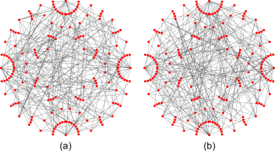
Figure 3: Networks after (a) $3\times 10^{5}$ and (b) $6\times 10^{5}$ operations of DR from the network shown by Fig. 1(b).

Examples of MD networks formed by DR’s from $G_{\text{ini}}$ shown in Fig. 1(b) are presented in Fig. 3. These networks seem to be very different from the $4$th generation $(2,2)$-flower ($G_{0}$) shown in Fig. 1(a), though the nearest-neighbor degree correlations are the same as $G_{0}$. In order to quantify such differences in network topology, we employ two indices. One is the spectral distance $U_{GG^{\prime}}$ between networks $G$ and $G^{\prime}$ with the same size $N$ Wilson08 ; Gu15 . The distance $U_{GG^{\prime}}$ is defined by

$$U_{GG^{\prime}}=\sqrt{\sum_{\alpha=1}^{N}\left[\left(\mu_{\alpha}^{G}-\mu_{\alpha}^{G^{\prime}}\right)^{2}+\left(\nu_{\alpha}^{G}-\nu_{\alpha}^{G^{\prime}}\right)^{2}\right]}.$$ (14)

Here, $\mu_{\alpha}^{G}$ and $\nu_{\alpha}^{G}$ are the $\alpha$th eigenvalues (in ascending order) of the adjacency matrix $A=[a_{ij}]$ and the Laplacian matrix $L=[l_{ij}]$, respectively, where $a_{ij}=1$ if the nodes $i$ and $j$ are connected in $G$, $a_{ij}=0$ otherwise, and $l_{ij}=-a_{ij}+\delta_{ij}\sum_{j^{\prime}}a_{ij^{\prime}}$. Since $U_{GG^{\prime}}$ is invariant under the similarity transform, $U_{GG^{\prime}}=0$ for networks $G$ and $G^{\prime}$ being isomorphic to each other. It should be remarked, however, that two cospectral networks providing $U_{GG^{\prime}}=0$ are not always isomorphic. Although $U_{GG^{\prime}}$ becomes large when the topology of $G^{\prime}$ largely deviates from $G$, it is not clear what type of topological differences strongly affects $U_{GG^{\prime}}$. Thus, we introduce another measure, the correlation distance $V_{GG^{\prime}}$, to quantify the topological difference between networks. The quantity $V_{GG^{\prime}}$ is defined as

$$V_{GG^{\prime}}=\frac{1}{2}\sum_{k,k^{\prime},l}\left|P_{G}(k,k^{\prime},l)-P_{G^{\prime}}(k,k^{\prime},l)\right|,$$ (15)

where $P_{G}(k,k^{\prime},l)$ is the joint probability that randomly chosen two nodes have the degrees $k$ and $k^{\prime}$ and are separated by the shortest path distance $l$ to each other. Similar to $U_{GG^{\prime}}$, $V_{GG^{\prime}}$ takes the minimum value $0$ if $G=G^{\prime}$. $V_{GG^{\prime}}$ becomes maximum if two distribution functions $P_{G}(k,k^{\prime},l)$ and $P_{G^{\prime}}(k,k^{\prime},l)$ have no overlap, and isbounded by $1$ because of the normalization condition$\sum_{k,k^{\prime},l}P_{G}(k,k^{\prime},l)=1$. A large correlation distance $V_{GG^{\prime}}$ implies that $G^{\prime}$ displays very different (long-range) degree correlations from $G$.

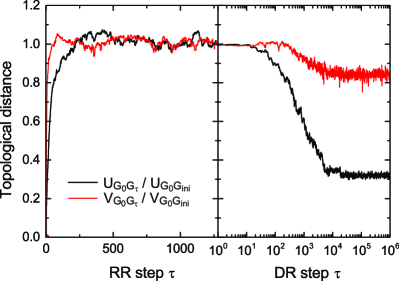
Figure 4: Spectral distance $U_{G_{0}G_{\tau}}$ (black line) and correlation distance $V_{G_{0}G_{\tau}}$ (red line) rescaled by $U_{G_{0}G_{\text{ini}}}$ and $V_{G_{0}G_{\text{ini}}}$, respectively, where $G_{0}$ is the 4th generation $(2,2)$-flower, and $G_{\text{ini}}$ is the network after $5M=1\,280$ operations of RR from $G_{0}$. The left panel displays the distances during $5M$ operations of RR starting from $G_{0}$, while the right panel shows the distance changes by DR’s starting from $G_{\text{ini}}$.

We examined how largely MD networks are different from the $(u,v)$-flower by computing the above topological distances. The left panel of Fig. 4 shows $U_{G_{0}G_{\tau}}$ and $V_{G_{0}G_{\tau}}$ as a function of the number of RR steps $\tau$, where $G_{0}$ is the original 4th generation $(2,2)$-flower $G_{4}^{(2,2)}$ and $G_{\tau}$ is the network after $\tau$ operations of RR from $G_{0}$. The right panel depicts the same quantities, but $\tau$ is the number of DR steps starting from $G_{\text{ini}}$, and $G_{\tau}$ is the network after $\tau$ operations of DR from $G_{\text{ini}}$. In this panel, data for $\tau\geq 18\,473$ represent the topological distances of MD networks from $G_{4}^{(2,2)}$. The topological distances must become zero at some values of $\tau$ in this region because the $G_{4}^{(2,2)}$ included in $S_{\text{MD}}$ is reachable from any MD network by DR’s. Nevertheless, both the spectral and correlation distances never drop to zero, at least within the present window of $\tau$. This implies that the topology of MD network in $S_{\text{MD}}$ is diverse and most of MD networks have very different structures from the $(u,v)$-flower.

The diverse topologies of MD networks can be readily understood through the idea of unit rewiring. The $n$th generation $(u,v)$-flower $G_{n}^{(u,v)}$ is composed of $w^{n-m}$ pieces of $G_{m}^{(u,v)}$ ($m\leq n$). If we regard $G_{m}^{(u,v)}$ as a superedge of $G_{n}^{(u,v)}$, $G_{n}^{(u,v)}$ is equivalent to $G_{n-m}^{(u,v)}$ with superedges. Let us perform RR operations for $G_{n-m}^{(u,v)}$ with superedges, which corresponds to RR’s in units of the subgraph $G_{m}^{(u,v)}$ in $G_{n}^{(u,v)}$. We call such a rewiring a unit rewiring (UR). As examples, networks after $320$ and $80$ operations of UR in units of $G_{1}^{(2,2)}$ and $G_{2}^{(2,2)}$ starting from $G_{4}^{(2,2)}$ are depicted in Figs. 5(a) and 5(b), respectively. It should be emphasized that the network after UR’s has the same $P(k,k^{\prime})$, and thus $\rho$, as the original network $G_{n}^{(u,v)}$. Therefore, all networks formed by UR’s are elements of $S_{\text{MD}}$. The number of networks formed by UR operations in units of $G_{m}^{(u,v)}$ starting from $G_{n}^{(u,v)}$ is equivalent to the number of networks with the same degree sequence as $G_{n-m}^{(u,v)}$. Since even this number is quite large Barvinok13 , the number of elements in $S_{\text{MD}}$ that includes unit-rewired networks as a part of it rises astronomically.

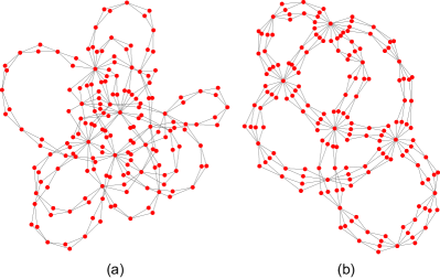
Figure 5: Networks after (a) $320$ and (b) $80$ operations of UR in units of $G_{1}^{(2,2)}$ and $G_{2}^{(2,2)}$ starting from $G_{4}^{(2,2)}$, respectively.

Considering the property of unit rewiring, in a network $G_{\text{UR}}$ formed by UR operations in units of $G_{m}^{(u,v)}$, the degree-degree correlation or other structural correlations in units of $G_{m}^{(u,v)}$ cannot extend beyond the scale of them. This implies that the network $G_{\text{UR}}$ ($\in S_{\text{MD}}$) does not possess the fractal property as a long-range structural correlation. Thus, we can conclude that disassortative degree mixing does not always make a scale-free network fractal. Although the $(u,v)$-flower in $S_{\text{MD}}$ has surely a fractal structure, it can be demonstrated that fractal networks are rather rare in the set $S_{\text{MD}}$. In the right panel of Fig. 6, the number of covering subgraphs $N_{\text{B}}$ [see Eqs. (1) and (2)] is plotted as a function of $l_{\text{B}}$ for $4$ topologically very different networks in $S_{\text{MD}}$, by employing the compact-box-burning algorithm Song07 . These results show that $N_{\text{B}}(l_{\text{B}})$ decreases exponentially with $l_{\text{B}}$. In addition to these $4$ examples, we examined $N_{\text{B}}(l_{\text{B}})$ for totally $100$ MD networks with different topologies to each other. Our results show that $N_{\text{B}}(l_{\text{B}})$ for every network obeys Eq. (1), which implies that most of MD networks with the scale-free property are not fractal, but have the small-world property.

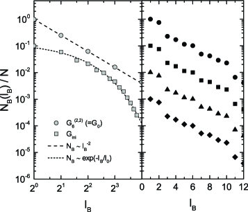
Figure 6: Number of covering subgraphs $N_{\text{B}}$ as a function of the subgraph diameter $l_{\text{B}}$ for the original 6th generation $(u,v)$-flower $G_{6}^{(2,2)}$ (gray circles in the left panel), $G_{\text{ini}}$ formed by RR’s from $G_{6}^{(2,2)}$ (gray squares in the left panel), and four topologically different networks in $S_{\text{MD}}$ formed by DR’s from $G_{\text{ini}}$ (black symbols in the right panel). The results are vertically shifted for graphical reasons. Lines in the left panel are guides to the eye.

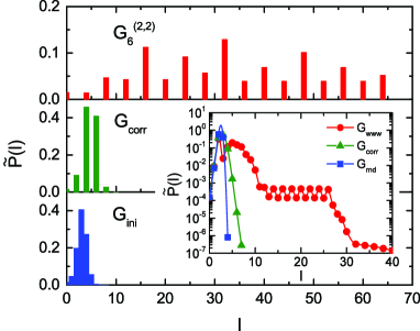
Figure 7: Distance distribution $\tilde{P}(l)$ for the 6th generation $(2,2)$-flower $G_{6}^{(2,2)}$ (top), networks ($G_{\text{corr}}$) formed by rewiring edges while keeping $P(k,k^{\prime})$ starting from $G_{6}^{(2,2)}$ (middle), and networks ($G_{\text{ini}}$) formed by RR’s starting from $G_{6}^{(2,2)}$ (bottom). The results for $G_{\text{corr}}$ and $G_{\text{ini}}$ are averaged over $100$ connected samples. The inset shows $\tilde{P}(l)$ for the WWW ($G_{\text{www}}$) with $N=325\,729$ nodes and $M=1\,497\,134$ edges URL_www (red circles), a network ($G_{\text{corr}}$) formed by rewiring edges while keeping $P(k,k^{\prime})$ starting from $G_{\text{www}}$ (green triangles), and a network ($G_{\text{rnd}}$) formed by RR’s starting from $G_{\text{www}}$ (blue squares). Curves are guides to the eye.

Does the degree correlation have nothing to do with the fractal property of a scale-free network? Our results demonstrate that at least the nearest neighbor disassortative degree correlation cannot be the origin of fractality in scale-free networks. However, as seen in Fig. 1(a), the $(u,v)$-flower has a distinguishing feature of a long-range repulsive correlation between the same degrees. This is not found in a typical MD network shown in Fig. 3. In particular, the long-range repulsion between hub nodes is found not only in the $(u,v)$-flower but also in other synthetic scale-free fractal networks Song06 . In order to quantify the repulsive correlation between hubs, we introduce the conditional probability $P(l|k,k^{\prime})$ of randomly chosen two nodes with degrees $k$ and $k^{\prime}$ being separated by the distance $l$ to each other. If setting $k=k^{\prime}=k_{\text{max}}$, this probability indicates the distribution of shortest path distance among nodes with the largest degree $k_{\text{max}}$ and gives information on the hub-hub repulsion. To improve the statistical reliability of this distribution, we define the distance distribution function $\tilde{P}(l)=c\sum_{k,k^{\prime}}^{{}^{\prime}}P(l|k,k^{\prime})P(k)P(k^{\prime})$, where $P(k)$ is the degree distribution, $\sum_{k,k^{\prime}}^{{}^{\prime}}$ represents the summation over degrees of the top 2% of high degree nodes, and $c$ is the normalization constant. As expected, $\tilde{P}(l)$ for the $(u,v)$-flower shown in the top panel of Fig. 7 is distributed in a wide range of $l$, which implies that high degree nodes are likely to be largely separated from each other. The middle panel of Fig. 7 indicates $\tilde{P}(l)$ for networks ($G_{\text{corr}}$) formed by rewiring many edges while keeping $P(k,k^{\prime})$ starting from the $(u,v)$-flower, where we should note that $G_{\text{corr}}$ is a MD network. The actual rewiring process can be done as follows: First we choose randomly two edges $(i_{1},j_{1})$ and $(i_{2},j_{2})$ with four different end nodes, where the degree of node $i_{1}$ is equal to the degree of node $i_{2}$, then rewire them to $(i_{1},j_{2})$ and $(i_{2},j_{1})$. The function $\tilde{P}(l)$ for $G_{\text{corr}}$ is distributed in a narrow range of small $l$. The width of the distribution is, however, slightly wider than that for $G_{\text{ini}}$ (bottom panel of Fig. 7) formed by RR’s starting from the $(u,v)$-flower. This is because higher degree nodes are never directly connected in $G_{\text{corr}}$. In addition to the $(u,v)$-flower, we examined $\tilde{P}(l)$ for the WWW URL_www as a real-world scale-free fractal network. This network exhibits disassortative degree mixing ($\rho=-0.11$) and is known to have the fractal dimension $D=4.41$ Kawasaki10 ; Song05 . As shown in the inset of Fig. 7, $\tilde{P}(l)$ for the WWW has a long tail. If the network is rewired while keeping $P(k,k^{\prime})$, $\tilde{P}(l)$ becomes much narrower than that for the original WWW as seen by triangles in the inset and the network loses fractality. These results suggest that the fractal property of a scale-free network requires a long-range repulsive correlation between similar degree nodes, particularly hub nodes.

IV CONCLUSIONS

We have studied the relation between fractality of scale-free networks and their degree correlations. Real-world and synthetic fractal scale-free networks are known to exhibit disassortative degree mixing in common. It is, however, not obvious whether a negative correlation between nearest neighbor degrees causes the fractal property of a scale-free network, though the possibility of disassortativity being the origin of fractality is suggested. In order to clarify this point, we examined maximally disassortative (MD) networks prepared by rewiring edges while keeping the degree sequence. For the preparation of MD networks, uncorrelated networks are first formed by rewiring randomly edges of the $(u,v)$-flower. Then, these networks are again rewired to minimize the rank correlation coefficient $\rho$. Our results show that there exist a huge number of MD networks with different topologies but most of them are not fractal. Therefore, it is concluded that negative correlations between nearest neighbor degrees cannot be the origin of fractality of scale-free networks. This can be readily understood if we consider MD networks formed by unit rewiring operations starting from the $(u,v)$-flower, because unit-rewired networks cannot have any structural correlations beyond the scale of the rewiring unit. In addition, we studied the long-range repulsion between hub nodes in fractal scale-free networks and their rewired networks while keeping the joint probability $P(k,k^{\prime})$. The results for the $(u,v)$-flower and a real-world fractal scale-free network show that distances between large degree nodes in fractal scale-free networks are much longer than those in their rewired networks. This fact prompts the speculation that fractality of scale-free networks requires a long-range repulsive correlation in similar degrees.

We should point out that networks treated in this work are a bit special. As mentioned in Sec. I, MD networks are generally composed of communities in each of which all nodes with a specific low degree and higher degree nodes are connected alternately. This gives MD networks a long-range degree correlation. On the other hand, an MD network with the same degree sequence as the $(u,v)$-flower ($u>1$) consists of only one community, because the total number of spokes from the lowest degree nodes is equal to or larger than that from all remaining higher degree nodes. We then cannot expect the long-range degree correlation in MD networks with the same degree sequence as the $(u,v)$-flower. Nevertheless, our conclusion is considered to be still valid even for more general networks. This is because disassortative degree mixing does not introduce any long-range repulsive correlations between similar degree nodes in a community of a general MD network. Therefore, the MD network is not fractal at least below the scale of the community.

Our speculation about the long-range repulsive correlation between similar degree nodes for fractal scale-free networks should be checked by further investigations. For this purpose, it is significant to define a new index characterizing the strength of such a repulsive correlation. It is interesting to identify whether a network formed by rewiring edges to maximize this index becomes fractal.

*

Appendix A $\rho$ OF THE $(u,v)$-FLOWER

Here, we derive Eq. (12) for the $n$th generation $(u,v)$-flower with $u\geq 2$ and $n\geq 2$. At first, we determine the rank $R_{k_{m}}$ for the degree $k_{m}=2^{m}$ ($m=1,2,\cdots,n$) in the $(u,v)$-flower. For the $(u,v)$-flower, Eq. (10) can be written as

$$R_{k_{m}}=\frac{S(k_{m})+1}{2}+\sum_{m^{\prime}=1}^{m-1}S(k_{m^{\prime}}),$$ (16)

where $S(k_{m})=k_{m}N_{k_{m}}$ is the total number of spokes from nodes with degree $k_{m}$. Since $N_{k_{m}}$ is given by Eq. (6), we have

$$S(k_{m})=\begin{cases}2^{m}(w-2)w^{n-m}&(1\leq m<n),\\ 2^{n}w&(m=n),\end{cases}$$ (17)

where $w=u+v$. Therefore, the rank of degree $k_{m}$ is presented by

$$R_{k_{m}}=\begin{cases}\displaystyle w^{n}\left[2-\biggl{(}\frac{w}{2}+1\biggr{)}\biggl{(}\frac{2}{w}\biggr{)}^{m}\right]+\frac{1}{2}&(1\leq m<n),\\[10.0pt] \displaystyle 2w^{n}-2^{n-1}w+\frac{1}{2}&(m=n).\end{cases}$$ (18)

To calculate $\rho$ by Eq. (11), we need to evaluate

$$X=\sum_{(i,j)\in E}R_{k_{i}}R_{k_{j}},$$ (19)

and

$$Y=\sum_{(i,j)\in E}\left(R_{k_{i}}^{2}+R_{k_{j}}^{2}\right),$$ (20)

for the $(u,v)$-flower. Considering that nodes with degree $k_{m}$ for $m\geq 2$ always connect to the lowest degree nodes with degree $k_{1}=2$, the number of edges whose end nodes have the degree ranks $R_{k_{m}}\ (m\geq 2)$ and $R_{k_{1}}$ is $S(k_{m})$. The remaining $\left[S(k_{1})-\sum_{m=2}^{n}S(k_{m})\right]/2$ edges connect the lowest degree nodes to each other. Thus, the quantity $X$ is presented by

$$X=\sum_{m=2}^{n}S(k_{m})R_{k_{m}}R_{k_{1}}+\frac{1}{2}\left[S(k_{1})-\sum_{m=2}^{n}S(k_{m})\right]R_{k_{1}}^{2}.$$ (21)

Using Eqs. (17) and (18), the quantity $X$ is calculated as

$$X=\left(1-z^{2}\right)M^{3}+M^{2}+\frac{1}{4}M,$$ (22)

where $z=2/w$ and the number of edges $M$ is given by $(2/z)^{n}$. The summation over edges in Eq. (20) is also rewritten as

$$Y=\sum_{m=1}^{n}S(k_{m})R_{k_{m}}^{2},$$ (23)

and $Y$ can be calculated as

$$Y=\frac{2(z+1)^{2}}{z^{2}+z+1}M^{3}+2M^{2}+\frac{1}{2}M-\frac{2z}{z^{2}+z+1}\frac{2^{3n}}{z^{3}}.$$ (24)

The calculations of Eqs. (22) and (24) become easier if we utilize the obvious relations $\sum_{m=1}^{n}S(k_{m})=2M$ and $\sum_{m=1}^{n}S(k_{m})R_{k_{m}}=M(2M+1)$. From Eqs. (11), (22) and (24), the rank correlation coefficient $\rho_{n}^{(u,v)}$ for the $n$th generation $(u,v)$-flower is then calculated as

$$\rho_{n}^{(u,v)}=-\frac{z\left(z^{2}+z+1\right)}{1-z^{3(n-1)}},$$ (25)

which is identical to Eq. (12). For the $(2,2)$-flower, for example, $\rho_{n}^{(2,2)}$ is calculated as

$$\rho_{n}^{(2,2)}=-\frac{7}{8}\left[1-\frac{1}{2^{3(n-1)}}\right]^{-1},$$ (26)

which gives $\rho_{\infty}=-7/8$ for $n\to\infty$.

The assortativity $r$ defined by Eq. (3) for the $n$th generation $(u,v)$-flower with $u\geq 2$ and $n\geq 2$ can be calculated by a similar way. The result is given by

$$r=\begin{cases}\displaystyle-\frac{2^{n+2}z^{n}-a^{2}(2z-1)-4}{(2z-1)(a^{2}-b)}&(w\neq 4,8),\\[15.0pt] \displaystyle-\frac{(n+1)^{2}-4n}{(3\cdot 2^{n}-2)-(n+1)^{2}}&(w=4),\\[15.0pt] \displaystyle-\frac{4^{n-1}-2^{n}+1}{4^{n-1}(3n-8)+3\cdot 2^{n}-1}&(w=8),\end{cases}$$ (27)

where

$$a=\frac{(2z)^{n}+2z-2}{2z-1},$$ (28)

and

$$b=\frac{3\cdot 4^{n}z^{n}+4z-4}{4z-1}.$$ (29)

For $n\to\infty$, the assortativity $r_{\infty}$ converges as

$$r_{\infty}=\begin{cases}0&(w\leq 8),\\ \displaystyle-\frac{2}{w(w-2)}&(w\geq 9).\end{cases}$$ (30)

Since the scale-free exponent $\gamma$ given by Eq. (7) is less than $4$ for $w\leq 8$, the above result is consistent with the general fact Menche10 ; Dorogovtsev10 ; Litvak13 that $r$ cannot be negative for infinitely large scale-free networks with $\gamma\leq 4$.

References

- (1) R. Albert and A.-L. Barabási, Rev. Mod. Phys. 74, 47 (2002).
- (2) S. N. Dorogovtsev, A. V. Goltsev, and J. F. F. Mendes, Rev. Mod. Phys. 80, 1275 (2008).
- (3) R. Pastor-Satorras, C. Castellano, P. Van Mieghem, and A. Vespignani, Rev. Mod. Phys. 87, 925 (2015).
- (4) A.-L. Barabási and R. Albert, Science 286, 509 (1999).
- (5) M. E. J. Newman, Phys. Rev. Lett. 89, 208701 (2002).
- (6) M. E. J. Newman, Phys. Rev. E 67, 026126 (2003).
- (7) F. Kawasaki and K. Yakubo, Phys. Rev. E 82, 036113 (2010).
- (8) D. J. Watts and S. H. Strogatz, Nature 393, 440 (1998).
- (9) C. Song, S. Havlin, and H. A. Makse, Nature 433, 392 (2005).
- (10) L. K. Gallos, C. Song, and H. A. Makse, Phys. Rev. Lett. 100, 248701 (2008).
- (11) L. K. Gallos, H. A. Makse, and M. Sigman, Proc. Natl. Acad. Sci. USA 109, 2825 (2012).
- (12) A. Watanabe, S. Mizutaka, and K. Yakubo, J. Phys. Soc. Jpn. 84, 114003 (2015).
- (13) S.-H. Yook, F. Radicchi, and H. Meyer-Ortmanns, Phys. Rev. E 72, 045105 (2005).
- (14) C. Song, S. Havlin, and H. A. Makse, Nat. Phys. 2, 275 (2006).
- (15) H. D. Rozenfeld, S. Havlin, and D. ben-Avraham, New J. Phys. 9, 175 (2007).
- (16) The -flower with is not fractal but has the small-world property, see S. N. Dorogovtsev, A. V. Goltsev, and J. F. F. Mendes, Phys. Rev. E 65, 066122 (2002).
- (17) J. S. Kim, B. Kahng, and D. Kim, Phys. Rev. E 79, 067103 (2009).
- (18) J. Menche, A. Valleriani, and R. Lipowsky, Phys. Rev. E 81, 046103 (2010).
- (19) C. M. Schneider, A. A. Moreira, J. S. Andrade, S. Havlin, and H. J. Herrmann, Proc. Natl. Acad. Sci. USA 108, 3838 (2011).
- (20) S. Johnson, J. J. Torres, J. Marro, and M. A. Muñoz, Phys. Rev. Lett. 104, 108702 (2010).
- (21) A. Bekessy, P. Bekessy, and J. Komlos, Stud. Sci. Math. Hungar. 7, 343 (1972).
- (22) M. Molloy and B. Reed, Random Struct. Algorithms 6, 161 (1995).
- (23) M. E. J. Newman, S. H. Strogatz, and D. J. Watts, Phys. Rev. E 64, 026118 (2001).
- (24) S. N. Dorogovtsev, L. Ferreira, V. Goltsev, and J. F. F. Mendes, Phys. Rev. E 81, 031135 (2010).
- (25) N. Litvak and R. van der Hofstad, Phys. Rev. E 87, 022801 (2013).
- (26) M. Raschke, M. Schlpfer, and R. Nibali, Phys. Rev. E 82, 037102 (2010).
- (27) W.-Y. Zhang, Z.-W. Wei, B.-H. Wang, and X.-P. Han, Physica A 451, 440 (2016).
- (28) L. Donetti, P. I. Hurtado, and M. A. Muñoz, Phys. Rev. Lett. 95, 188701 (2005).
- (29) R. C. Wilson and P. Zhu, Patt. Recog. 41, 2833 (2008).
- (30) J. Gu, B. Hua and S. Liu, Discrete Appl. Math. 190-191, 56 (2015).
- (31) A. Barvinok and J. A. Hartigan, Random Struct. Algor. 42, 301 (2013).
- (32) C. Song, L. K. Gallos, S. Havlin, and H. A. Makse, J. Stat. Mech.: Theory Exp. (2007), P03006.
- (33) http://konect.uni-koblenz.de/networks/moreno_propro.