Velocity Distribution of Driven Inelastic One-component Maxwell gas

Abstract

The nature of the velocity distribution of a driven granular gas, though well studied, is unknown as to whether it is universal or not, and if universal what it is. We determine the tails of the steady state velocity distribution of a driven inelastic Maxwell gas, which is a simple model of a granular gas where the rate of collision between particles is independent of the separation as well as the relative velocity. We show that the steady state velocity distribution is non-universal and depends strongly on the nature of driving. The asymptotic behavior of the velocity distribution are shown to be identical to that of a non-interacting model where the collisions between particles are ignored. For diffusive driving, where collisions with the wall are modelled by an additive noise, the tails of the velocity distribution is universal only if the noise distribution decays faster than exponential.

I Introduction

Granular matter, constituted of particles that interact through inelastic collisions, exhibit diverse phenomena such as cluster formation, jamming, phase separation, pattern formation, static piles with intricate stress networks, etc. Jaeger et al. (1996); Aranson and Tsimring (2006); Goldhirsch and Zanetti (1993); Li et al. (2003); Corwin et al. (2005). Its ubiquity in nature and in industrial applications makes it important to understand how the macroscopically observed behavior of granular systems arises from the microscopic dynamics. A well studied macroscopic property is the velocity distribution of a dilute granular gas. While several studies (see below) have shown that the inherent non-equilibrium nature of the system, induced by inelasticity, could result in a non-Maxwellian velocity distribution, they fail to pinpoint whether the velocity distribution is universal, and if yes, what its form is. In this paper, we focus on the role of driving in determining the velocity distribution within a simplified model for a granular gas, namely the inelastic Maxwell model.

Dilute granular gases are of two kinds: freely cooling in which there is no input of energy Haff (1983); Brey et al. (1996); Esipov and Pöschel (1997); Ben-Naim et al. (1999); Ben-Naim and Krapivsky (2000); van Noije and Ernst (1998); Nie et al. (2002); Dey et al. (2011); Pathak et al. (2014a, b); Shinde et al. (2007), or driven, in which energy is injected at a constant rate. In the freely cooling granular gas, the velocity distribution at different times $t$ has the form $P(v,t)\simeq v^{-1}_{rms}f(v/v_{rms})$, where $v$ is any of the velocity components, $v_{rms}(t)$ is the time dependent root mean square velocity and $f$ is a scaling function. $v_{rms}(t)$ decreases in time as a power law $v_{rms}(t)\sim t^{-\theta}$. To determine the behavior of $f$ for large argument, it was argued that the contributions to the tails of the velocity distributions are from particles that do not undergo any collisions, implying an exponential decay of $P(v,t)$ with time $t$ Nie et al. (2002). Thus, $f(x)\sim\exp(-ax^{1/\theta})$, or $P(v,t)\sim e^{-av^{1/\theta}t}$ for large $v$. It is known that at initial times, the granular particles remain homogeneously distributed with $\theta=1$ Haff (1983), leading to $P(v,t)$ having an exponential decay in all dimensions. At late times they tend to cluster resulting in density inhomogeneities with current evidence suggesting $\theta=d/(d+2)$  Ben-Naim et al. (1999); Nie et al. (2002); Pathak et al. (2014b).

In dilute driven granular gases, the focus of this paper, the system reaches a steady state where the energy lost in collisions is balanced by external driving. Several experiments, simulations and theoretical studies have focused on determining the steady state velocity distribution $P(v)$. In experiments, driving is done either mechanically Clement and Rajchenbach (1991); Warr et al. (1995); Kudrolli et al. (1997); Olafsen and Urbach (1999); Losert et al. (1999); Kudrolli and Henry (2000); Blair and Kudrolli (2001); Rouyer and Menon (2000) through collision of the particles with vibrating wall of the container or by applying electric Aranson and Olafsen (2002) or magnetic fields Kohlstedt et al. (2005) on the granular beads. Almost all the experiments find the tails of $P(v)$ to be non-Maxwellian, and described by a stretched exponential form $P(v)\sim\exp(-av^{\beta})$ for large $v$. Some of these experiments find $P(v)$ to be universal with $\beta=3/2$ for a wide range of parameters Losert et al. (1999); Rouyer and Menon (2000). In contrast, other experiments Olafsen and Urbach (1999); Blair and Kudrolli (2001) find $P(v)$ to be non-universal with the exponent $\beta$ varying with the system parameters, sometimes even approaching a Gaussian distribution ($\beta=2$) Olafsen and Urbach (1999).

In numerical simulations, driving is done either from the boundaries Du et al. (1995); Esipov and Pöschel (1997) which leads to clustering, or homogeneously Williams and MacKintosh (1996); Moon et al. (2001); van Zon and MacKintosh (2004, 2005) within the bulk. In simulations of a granular gas in three dimensions, driven homogeneously by addition of white noise to the velocity (diffusive driving), it was observed that $\beta=3/2$ for large enough inelasticity Moon et al. (2001). However, similar simulations of a bounded two dimensional granular gases with diffusive driving found a range of distributions in the steady state, with $\beta$ ranging from $0.7$ to $2$ as the parameters in the system are varied van Zon and MacKintosh (2004, 2005).

Theoretical approaches have been of two kinds: kinetic theory, or by studying simple models which capture essential physics but are analytically tractable. In kinetic theory Brilliantov and Pöschel (2004), the Boltzmann equation describing the evolution of the distribution function is obtained by truncating the BBGKY hierarchy by assuming product measure for joint distribution functions. While it is difficult to solve this non-linear equation exactly, the deviation of the velocity distribution from Gaussian can be expressed as a perturbation expansion using Sonine polynomials Goldshtein and Shapiro (2006); van Noije and Ernst (1998); Brilliantov and Pöschel (2004); Dubey et al. (2013). This approach describes the velocity distribution near the typical velocities. The tails of the distribution can be obtained by linearizing the Boltzmann equation van Noije and Ernst (1998); Montanero and Santos (2000); Barrat et al. (2002). Notably, for granular gases with diffusive driving, this leads to the prediction $P(v)\simeq{\mathcal{C}}\exp(-b|v|^{\beta})$ with $\beta=3/2$ for large velocities, independent of the coefficient of restitution, strongly suggesting that the velocity distribution is universal van Noije and Ernst (1998).

The alternate theoretical approach is to study simpler model like the inelastic Maxwell gas, in which spatial coordinates of the particles are ignored and each pair of particles collide at constant rate Ben-Naim and Krapivsky (2000). In the freely cooling Maxwell gas, the velocity distribution decays as a power law with an exponent that depends on dimension and coefficient of restitution Baldassarri et al. (2002); Ernst and Brito (2002a); Krapivsky and Ben-Naim (2002); Ben-Naim and Krapivsky (2002). In contrast, for a diffusively driven Maxwell gas, in which collisions with the wall and modelled by velocities being modified by an additive noise, it was shown that $P(v)$ has a universal exponential tail ($\beta=1$) for all coefficients of restitution Ernst and Brito (2002b); Antal et al. (2002). However, it has been recently shown Prasad et al. (2013, 2014) that when the driving is diffusive, the velocity of the center of mass does a Brownian motion, and the total energy increases linearly with time at large times. Thus, the system fails to reach a time-independent steady state, making the results for diffusive driving valid only for intermediate times when a pesudo-steady state might be assumed. This drawback may be overcome by modeling driving through collisions with a wall, where the new velocity $v^{\prime}$ of a particle colliding with a wall is given by $v^{\prime}=-r_{w}v+\eta$, where $r_{w}$ is the coefficient of restitution for particle-wall collisions, and $\eta$ is uncorrelated noise representing the momentum transfer due to the wall Prasad et al. (2013) (diffusive driving corresponds to $r_{w}=-1$). For this dissipative driving ($|r_{w}|<1$), the system reaches a steady state, and the velocity distribution was shown to be Gaussian when $\eta$ is taken from a normalized Gaussian distribution Prasad et al. (2013). If $\eta$ is described by a Cauchy distribution, the steady state $P(v)$ is also a Cauchy distribution, but with a different parameter Prasad et al. (2013).

Thus, while the velocity distribution for the freely cooling granular gas is universal and reasonably well understood, it has remained unclear whether the velocity distribution of a driven granular gas is universal. Also, if the velocity distribution is non-Maxwellian, a clear physical picture for its origin is missing. Intuitively, it would appear that the tails of the velocity distribution would be dominated by particles that have been recently driven and not undergone any collision henceforth. This would mean the $P(v)$ cannot decay faster than the distribution of the noise associated with the driving. If this reasoning is right, the noise statistics should play a crucial role in determining the velocity distribution, making it non-universal. How sensitive is $P(v)$ to the details of the driving? In particular, how does $P(v)$ behave for large $v$ for different noise distributions $\Phi(\eta)$? We answer this question within the Maxwell model, both for dissipative driving ($0\leq r_{w}<1$) as well as the pseudo steady state for diffusive driving ($r_{w}=-1$). In particular, we show that the tail statistics are determined by the noise distribution for dissipative driving. For the pseudo steady state in diffusive driving, we find that the velocity distribution is universal if the noise distribution decays faster than exponential and determined by noise statistics if the noise distribution decays slower than exponential.

The rest of the paper is organized as follows. In Sec. II we define the Maxwell model and its dynamics more precisely. In Sec. III the steady state velocity distribution of the system are determined by studying its characteristic function as well as the asymptotic behavior of ratios of successive moments. In particular, we obtain the velocity distribution for a family of stretched exponential distributions for the noise. The results for dissipative driving may be found in Sec. III.1 and those for diffusive driving in Sec. III.2. In Sec. IV, the exact solution of the non-interacting problem is presented. Section V contains a summary and discussion of results.

II Driven Maxwell gas

Consider $N$ particles of unit mass. Each particle $i$ has a one-component velocity $v_{i}$, $i=1,2,\ldots,N$. The particles undergo two-body collisions that conserve momentum but dissipate energy, such that when particles $i$ and $j$ collide, the post-collision velocities $v_{i}^{\prime}$ and $v_{j}^{\prime}$ are given in terms of the pre-collision velocities $v_{i}$ and $v_{j}$ as:

$$\begin{split}v_{i}^{\prime}&=\frac{(1-r)}{2}v_{i}+\frac{(1+r)}{2}v_{j},\\ v_{j}^{\prime}&=\frac{(1+r)}{2}v_{i}+\frac{(1-r)}{2}v_{j},\end{split}$$ (1)

where $r\in[0,1]$ is the coefficient of restitution. For energy-conserving elastic collisions, $r=1$. In the Maxwell gas, the rate of collision of a pair of particles is assumed to be independent of their spatial separation as well as their relative velocity. These simplifying assumptions make the model more tractable as the spatial coordinates of the particles may now be ignored.

The system is driven by input of energy, modeled by particles colliding with a vibrating wall Prasad et al. (2013). If particle $i$ with velocity $v_{i}$ collides with the wall having velocity $V_{w}$, the new velocities $v^{\prime}_{i}$, $V^{\prime}_{w}$ respectively, satisfy the relation $v_{i}^{\prime}-V_{w}^{\prime}=-r_{w}(v_{i}-V_{w})$, where the parameter $r_{w}$ is the coefficient of restitution for particle-wall collisions. Since the wall is much heavier than the particles, $V_{w}^{\prime}\approx V_{w}$, and hence $v_{i}^{\prime}=-r_{w}v_{i}+(1+r_{w})V_{w}$. Since the motion of the wall is independent of the particles and the particle-wall collision times are random, it is reasonable to replace $(1+r_{w})V_{w}$ by a random noise $\eta$ and the new velocity $v_{i}^{\prime}$ is now given by Prasad et al. (2013),

$$v_{i}^{\prime}=-r_{w}v_{i}+\eta_{i}.$$ (2)

In this paper, we consider a class of normalized stretched exponential distributions for the noise $\eta$,

$$\Phi(\eta)=\frac{a^{\frac{1}{\gamma}}}{2\Gamma\left(1+\frac{1}{\gamma}\right)}\exp(-a|\eta|^{\gamma})~{}a,\gamma>0,$$ (3)

characterized by the exponent $\gamma$. Note that there is no apriori reason to assume that the noise is Gaussian as the noise is not averaged over many random kicks.

The system is evolved in discrete time steps. At each step, a pair of particles are chosen at random and with probability $p$ they collide according to Eq. (1), and with probability $(1-p)$, they collide with the wall according to Eq. (2). We note that evolving the system in continuous time does not change the results obtained for the steady state.

We also note that though the physical range of $r_{w}$ is $[0,1]$, it is useful to mathematically extend its range to $[-1,1]$. This makes it convenient to treat special limiting cases in one general framework. For instance, when $r_{w}=-1$, the driving reduces to a random noise being added to the velocities, corresponding to diffusive driving. In this case, the system reaches a pseudo-steady state before energy starts increasing linearly with time for large times Prasad et al. (2013, 2014). When $r_{w}\neq-1$, the system reaches a steady state that is independent of the initial conditions. In the limit $r_{w}\to-1$, and rate of collisions with the wall going to infinity, the problem reduces to an Ornstein-Uhlenbeck process Prasad et al. (2014). The case $r_{w}=1$ is also interesting. When $r_{w}=1$, the structure of the equations obeyed by the steady state velocity distribution is identical to those obeyed by the distribution in the pseudo-steady state of the Maxwell gas with diffusive driving ($r_{w}=-1$) Prasad et al. (2013).

III Steady state Velocity Distribution

We use two diagnostic tools to obtain the tail of the steady state velocity distribution: (1) by directly studying the characteristic function of the velocity distribution and (2) by determining the ratios of large moments of the velocity distribution.

In the steady state, due to collisions being random, there are no correlations between velocities of two different particles in the thermodynamic limit. We note that for finite systems, there are correlations that are proportional to $N^{-1}$ Prasad et al. (2013). The two point joint probability distributions can thus be written as a product of one-point probability distributions. It is then straightforward to write

$$P(v,t+1)=p\!\!\int\!\!\!\!\int\!\!dv_{1}dv_{2}P(v_{1},t)P(v_{2},t)\delta\left[\frac{1-r}{2}v_{1}+\frac{1+r}{2}v_{2}-v\right]+(1-p)\!\!\int\!\!\!\!\int\!\!d\eta dv_{1}\Phi(\eta)P(v_{1},t)\delta\left[\eta-r_{w}v_{1}-v\right],$$ (4)

where the first term on the right hand side describes the evolution due to collisions between particles and the second term describes the evolution due to collision between particles and wall. In the steady state, the velocity distributions become time independent and we use the notation $\lim_{t\to\infty}P(v,t)=P(v)$. Equation (4) is best analyzed in the Fourier space. Let the characteristic function of the velocity distribution be defined as

$$Z(\lambda)=\langle\exp(-i\lambda v)\rangle.$$ (5)

It can be shown from Eq. (4) that $Z(\lambda)$ satisfies the relation Prasad et al. (2013)

$$Z(\lambda)=pZ\left(\frac{[1-r]\lambda}{2}\right)Z\left(\frac{[1+r]\lambda}{2}\right)+(1-p)Z(r_{w}\lambda)f(\lambda),$$ (6)

where $f(\lambda)\equiv\langle\exp(-i\lambda\eta)\rangle_{\eta}$. Equation (6) is non-linear and non-local (in the argument of $Z$) and is not solvable in general. But it is possible to numerically obtain the probability distribution for certain choices of the parameters.

When $r=0$ and $r_{w}=1/2$, Eq. (6) takes the form,

$$Z(\lambda)=p\left[Z\left(\frac{\lambda}{2}\right)\right]^{2}+(1-p)Z\left(\frac{\lambda}{2}\right)f(\lambda),~{}r=0,r_{w}=\frac{1}{2}.$$ (7)

Thus, $Z(\lambda)$ is determined if $Z(\lambda/2)$ is known. By iterating to smaller $\lambda$, and considering the initial value $Z(\lambda)=1-\lambda^{2}\langle v^{2}\rangle/2$ for small $\lambda$, one can use this recursion relation to calculate characteristic function for any value of $\lambda$. Here $\langle v^{2}\rangle$ may be calculated exactly [see Eq. (9)]. The velocity distribution may be obtained from the inverse Fourier transform of $Z(\lambda)$.

When $r_{w}=1$, Eq. (6) allows the tail statistics of $P(v)$ to be determined exactly. In this case, the characteristic function satisfies the relation

$$Z(\lambda)=\frac{pZ\left([1-r]\lambda/2\right)Z\left([1+r]\lambda/2\right)}{[1-(1-p)f(\lambda)]},~{}~{}r_{w}=1.$$ (8)

Equation (8) may be iteratively solved to obtain an infinite product involving simple poles. The behavior of the velocity distribution for asymptotically large velocities is determined by the pole closest to the origin, and has the form $P(v)\sim\exp(-\lambda^{*}|v|)$, where $\lambda^{*}$ is determined from $1-(1-p)f(\lambda)=0$ Prasad et al. (2013). When $r=1/2$, the iterative numerical scheme discussed above for dissipative driving may be followed for determining the characteristic function for the diffusive case.

The dynamics [Eqs.(1,2)] also allows the calculation of the moments of the steady state distribution. For the Maxwell model, it was shown that the equations for the two point correlation functions close Prasad et al. (2013, 2014). The closure can be also extended to one dimensional pseudo Maxwell models where particles collide only with nearest neighbor particles with equal rates Prasad et al. (2016). Using this simplifying property, the variance of the steady state velocity distribution in the thermodynamic limit was determined to be:

$$\langle v^{2}\rangle=\frac{2\kappa\sigma^{2}}{1-r^{2}+2\kappa(1-r_{w}^{2})},$$ (9)

where $\kappa=(1-p)/p$ and $\sigma^{2}$ is the variance of the noise distribution. On the other hand, the two-point velocity correlations in the steady state vanishes in the thermodynamic limit.

Among the higher moments, the odd moments vanish as the velocity distributions is even. Define $2n$-th moment of the distribution to be $\langle v^{2n}\rangle=M_{2n}$. The evolution equation for $M_{2n}$ may be obtained by multiplying Eq. (4) by $v^{2n}$, and integrating over the velocities. It is then straightforward to show that they satisfy a recurrence relation,

$$\Bigl{[}1- \epsilon^{2n}-(1-\epsilon)^{2n}+\kappa\bigl{(}1-r_{w}^{2n}\bigr{)}\Bigr{]}\,M_{2n}=$$

$$\sum_{m=1}^{n-1}\binom{2n}{2m}\epsilon^{2m}(1-\epsilon)^{2n-2m}M_{2m}M_{2n-2m}$$

$$+\kappa\sum_{m=0}^{n-1}\binom{2n}{2m}r_{w}^{2m}M_{2m}N_{2n-2m},$$ (10)

where $\epsilon=(1-r)/2$ and $N_{i}$ is the $i$-th moment of the noise distribution. Equation (III) expresses $M_{2n}$ in terms of lower order moments. Since $P(v)$ is a normalizable distribution, $M_{0}=1$. Also $M_{2}$ is given by Eq. (9). Knowing these two moments, all higher order moments may be derived recursively using Eq. (III).

The ratios of moments may be used for determining the tail of the velocity distribution. Suppose the velocity distribution is a stretched exponential:

$$P(v)=\frac{b^{1/\beta}}{2\Gamma\left(1+\beta^{-1}\right)}\exp(-b|v|^{\beta}),~{}b,\beta>0,$$ (11)

where $\Gamma$ is the Gamma function. For this distribution the $2n^{th}$ moment is

$$M_{2n}=b^{-2n/\beta}\frac{\Gamma(\frac{2n+1}{\beta})}{\beta\Gamma(1+\frac{1}{\beta})},$$ (12)

such that that the ratios for large $n$ is

$$\frac{M_{2n}}{M_{2n-2}}\approx\left(\frac{2n}{b\beta}\right)^{2/\beta},~{}~{}n\gg 1.$$ (13)

Though Eq. (13) has been derived for the specific distribution given in Eq. (11), the moment ratios will asymptotically obey Eq. (13) even if only the tail of the distribution is a stretched exponential. This is because large moments are determined only by the tail of the distribution. Thus, the exponent $\beta$ can be obtained unambiguously from the asymptotic behavior of the moment ratios.

III.1 Dissipative Driving ($r_{w}<1$)

We first evaluate the velocity distribution numerically by inverting the characteristic function $Z(\lambda)$. For this calculation, $f(\lambda)$, the Fourier transform of the noise distribution in Eq. (3), is determined numerically using Eq. (7). Figure 1 shows the velocity distributions obtained for $\gamma=1/2,1,2,3$ for fixed $a=3$ (see Eq. (3) for definition of $a$). For the case $r_{w}=1/2$, corresponding to dissipative driving, the velocity distribution $P(v)$ approaches the noise distribution for large velocities for all values of $\gamma$. This suggests that the tail of the distribution is determined by the characteristics of the noise. However, using this method, it is not possible to extend the range of $v$ to larger values so that the large $v$ behavior may be determined unambiguously. The range of $v$ is limited by the precision to which $f(\lambda)$ can be determined numerically.

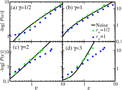
Figure 1: (color online) The numerically calculated velocity distribution $P(v)$, obtained from the inverse Fourier Transform of the characteristic function $Z(\lambda)$, for different noise distributions as described in Eq. (3) with (a) $\gamma=1/2$, (b) $\gamma=1$, (c) $\gamma=2$, and (d) $\gamma=3$ for $a=3$. $P(v)$ is computed for $r_{w}=1/2$ (dissipative driving) and $r_{w}=1$ (diffusive driving) and compared with the noise distribution.

The ratios of moments [see Eq. (13)] is a more robust method for determining the tail of the velocity distribution. The moments are calculated from the recurrence relation Eq. (III) where the moments of the noise distribution described in Eq. (3) is given by

$$N_{2n}=a^{-2n/\gamma}\frac{\Gamma(\frac{2n+1}{\gamma})}{\gamma\Gamma(1+\frac{1}{\gamma})}.$$ (14)

The numerically obtained moment ratios of the steady state velocity distribution for dissipative driving is shown in Fig. 2, for different noise distributions characterized by $\gamma$. The moment ratios increase with $n$ as a power law with an exponent $2/\gamma$, independent of the value of $r_{w}$ and the coefficient of restitution $r$. Comparing with Eq. (13), we obtain $\beta=\gamma$, and that the tail of the velocity distribution is determined by the noise distribution. We also compare the results with those for driven non-interacting particles. Here, collisions between particles are completely ignored so that the time evolution of particles are independent of each other, and each particle is driven independently. For the range of parameters, considered, the moment ratios of the interacting system is asymptotically indistinguishable from that of the non-interacting system, showing that for dissipative driving collisions between particles do not affect the tails of the velocity distribution. The moment ratios are also compared with those of the noise distribution. Here, we observe that while the ratios have the same power law exponent, the prefactor is different.

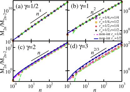
Figure 2: (Color Online) The moment ratios [see Eq. (13)] for different noise distributions as described in Eq. (3) with (a) $\gamma=1/2$, (b) $\gamma=1$, (c) $\gamma=2$, and (d) $\gamma=3$ for $a=3$. In each figure the ratios are plotted for $r=1/4,~{}1/2$, as well as $r_{w}=1/4,~{}1/2$, corresponding to dissipative driving. These are is compared with the moment ratios of the non-interacting system in which collisions are ignored, as well as the noise distribution (dashed green line).

We now determine the constant $b$ in the exponential in Eq. (11). It may be determined from Eq. (13) once $\beta$ is determined. Rearranging Eq. (13), we obtain

$$b(n)\approx\frac{2n}{\beta}\left(\frac{M_{2n}}{M_{2n-2}}\right)^{-\beta/2},~{}~{}n\gg 1.$$ (15)

Figures 3 (a) and(b) show the variation of $b(n)$ with $n$ for different $\gamma$. We find that for large $n$, $b(n)$ is independent of coefficient of restitution $r$, but may depend on $r_{w}$. Also, we find that $b-b(n)\propto n^{-1}$ for all values of $\gamma$. Figures 3 (c) and(f) show the variation of $b$ with $r_{w}$ for different $\gamma$. For $\gamma=1/2$ and $1$, $b$ is independent of $r_{w}$, while for $\gamma=2$ and $3$, it depends on $r_{w}$. We have checked that $b$ is independent of $r_{w}$ for $\gamma$ up to $1$. In Figures 3 (c) and(f), the values of $b$ are also compared with that obtained for a non-interacting system in which collisions between particles are ignored. We find that the values of $b$ for both the interacting and non-interacting system coincide. In addition, for $\gamma\leq 1$, we find that the value of $b$ approaches the value $a$ characterizing the noise distribution.

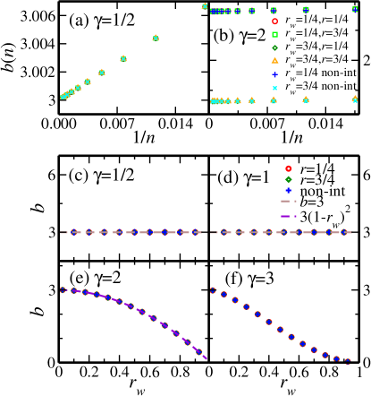
Figure 3: (Color Online) The coefficient $b(n)$ obtained from Eq. (15) for (a) $\gamma=1/2$, (b) $\gamma=2$ varies linearly with $n^{-1}$ for dissipative driving $r_{w}<1$. The choice of $r$ and $r_{w}$ are the same in both plots and labeled in (b). The corresponding $b(n)$ obtained for the non-interacting system are also shown. The variation of $b=b(\infty)$ with $r_{w}$ is shown for (c) $\gamma=1/2$, (d) $\gamma=1$, (e) $\gamma=2$ and (f) $\gamma=3$.

III.2 Velocity distributions for diffusive driving

The Maxwell gas with diffusive driving ($r_{w}=-1$) does not have a steady state in the long time limit, when the total energy diverges. However, it has a pseudo steady state solution that is valid at intermediate times. On the other hand when $r_{w}=1$ the system reaches a steady state at large time. It has been shown that the velocity distribution in the pseudo steady state for the case $r_{w}=-1$ is the same as the velocity distribution in the steady state of the system with $r_{w}=1$ Prasad et al. (2013). For $r_{w}=1$ and $\eta$ taken from a Gaussian distribution, the velocity distribution was shown to have an exponential distribution Prasad et al. (2013). In this section, we determine this steady state for other noise distributions.

In Fig. 1, the numerically obtained $P(v)$ is shown for different values of $\gamma$. We find that for $\gamma=1/2,1$ the velocity distribution approaches the noise distribution. Interestingly, when $\gamma=2,3$ the velocity distribution deviates significantly from the noise distribution. While the data for $\ln P(v)$ appears to vary linearly with $v$, the range is limited and it is not possible to unambiguously conclude that $P(v)$ is exponential independent of the noise distribution.

As for the dissipative case, the better tool to probe the tail of the distributions is the moment ratios Eq. (13). Figure 4 shows that moment ratios increase with $n$ as a power law. The power law exponent is $2/\gamma$ for $\gamma<1$ [see Fig. 4(a)] and equal to 2 for $\gamma\geq 1$ [see Fig. 4((b)-(d)]. Thus, we conclude that $\beta=\min[\gamma,1]$. Thus, $P(v)$ is universal, and has an exponential tail for $\gamma\geq 1$.

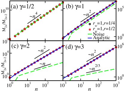
Figure 4: (color online) The moment ratios [see Eq. (13)] for different noise distributions as described in Eq. (3) with (a) $\gamma=1/2$, (b) $\gamma=1$, (c) $\gamma=2$, and (d) $\gamma=3$ for $a=3$. The data are for $r_{w}=1$ (diffusive driving) and the ratios are plotted for $r=1/4$,and $1/2$. These are compared with the noise distribution (dashed green line). In (b), (c) and (d), we also plot moment ratios for the exponential distribution with analytically obtained value of $\lambda^{*}$ [See Eqs. (16), (17)].

The exact form of the universal exponential tail can be analytically obtained as follows. If the velocity distribution has the form $P(v)=(\lambda^{*}/2)\exp(-\lambda^{*}|v|)$, the moment ratios in the large $n$ limit behaves as $M_{2n}/M_{2n-2}\approx(4n^{2}-2n)/(\lambda^{*})^{2}$. But we have seen in Sec. III that, for diffusive driving Eq. (8) satisfies a solution such that the velocity distribution is determined by the pole nearest to the origin $\pm i\lambda^{*}$ obtained from relation $1=(1-p)f(\lambda)$. When $\gamma=1$, the pole has the form given by

$$\lambda^{*} = \pm a\sqrt{p},~{}\gamma=1,$$ (16)

$$\lambda^{*} = \pm\frac{\sqrt{-2\ln(1-p)}}{\sigma},~{}\gamma=2.$$ (17)

When $\gamma=3$, we obtain complicated Hypergeometric function for $f(\lambda)$ from which $\lambda^{*}$ may be determined numerically. The moment ratios thus obtained are plotted in Fig. 4(b), (c), and (d) which matches with the numerically calculated moment ratio. It can be seen that when $\gamma<1$, there is no $\lambda^{*}$ which satisfies the relation $1=(1-p)f(\lambda)$.

From Eq. (15), we obtain the coefficient $b$ for the diffusively driven system and is shown in Fig. 5. It is seen that when $\gamma<1$, the coefficient $b(n)$ approaches that of the noise distribution $a=3$. For $\gamma\geq 1$, $b$ is calculated by substituting $\beta=1$ in Eq. (15). One finds in this case that $b$ approaches $\lambda^{*}$ which is obtained analytically.

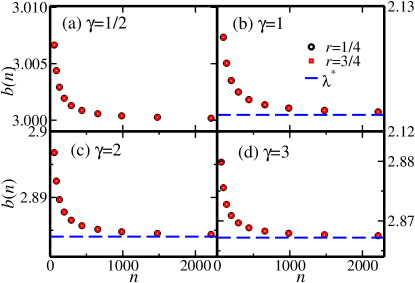
Figure 5: (Color Online) The variation of the coefficient $b(n)$ with $n$ obtained from Eq. (15) for diffusive driving $r_{w}=1$ and for different values of $r$, for different noise distribution characterized by (a) $\gamma=1/2$, (b) $\gamma=1$, (c) $\gamma=2$, (d) $\gamma=3$. The dashed line corresponds to the analytically obtained asymptotic value $\lambda^{*}$ [See Eqs. (16), (17)].

IV Non-interacting system

We showed in Sec. III.1 that, for dissipative driving, the tail of the velocity distribution $P(v)$ is identical to that of a non-interacting system in which collisions between particles may be ignored. In this section, we determine the velocity distribution of the non-interacting system in terms of the noise distribution. In the non-interacting system, the particle is driven at each time step. If $v_{n}$ is the velocity after the $n^{th}$ collision, then

$$v_{n}=-r_{w}v_{n-1}+\eta_{n-1}.$$ (18)

For a particle that is initially at rest ($v_{0}=0$),

$$v_{n}=\displaystyle\sum_{m=0}^{n-1}r_{w}^{m}\eta_{n-m-1}=\displaystyle\sum_{m=0}^{n-1}r_{w}^{m}\eta_{m},$$ (19)

where the second equality is in the statistical sense, and follows from the fact that noise is uncorrelated and therefore the order is irrelevant.

Now, consider the moment generating function of the noise distribution, $\langle\exp(-\lambda\eta)\rangle\equiv\exp[\mu(\lambda)]$ where $\mu(\lambda)$ is the cumulant generating function,

$$\mu(\lambda)\equiv\displaystyle\sum_{i=1}^{\infty}\frac{\lambda^{2n}}{2n!}C_{2n},$$ (20)

where $C_{2n}$ is the $2n^{\text{th}}$ cumulant of the noise distribution. It has been assumed that the noise distribution is symmetric such that only even cumulants are non-zero. The moment generating function of the velocity after infinite time-steps is,

$$\langle\exp(-\lambda v_{\infty})\rangle_{\eta} = \left\langle\exp\left[-\lambda\sum_{m=0}^{\infty}r_{w}^{m}\eta_{m}\right]\right\rangle_{\eta},$$

$$= \exp\left[-\sum_{m=0}^{\infty}\mu(r_{w}^{m}\lambda)\right].$$ (21)

From the definition of $\mu(\lambda)$ [see Eq. (20)], we obtain

$$\mu(r_{w}^{m}\lambda)=\displaystyle\sum_{n=1}^{\infty}\frac{(r_{w}^{m}\lambda)^{2n}}{2n!}C_{2n}.$$ (22)

Summing over $m$,

$$\sum_{m=0}^{\infty}\mu(r_{w}^{2m}\lambda) = \sum_{m=0}^{\infty}\sum_{n=1}^{\infty}\frac{(r_{w}^{m}\lambda)^{2n}}{2n!}C_{2n},$$

$$= \sum_{n=1}^{\infty}\frac{\lambda^{2n}}{2n!}\left(\frac{1}{1-r_{w}^{2n}}\right)C_{2n}.$$ (23)

But, $\langle\exp(-\lambda v_{\infty})\rangle=\exp\left[\xi(\lambda)\right]$ where $\xi(\lambda)$ is the cumulant generating function of the velocity distribution at large times,

$$\xi(\lambda)=\displaystyle\sum_{n=1}^{\infty}\frac{\lambda^{2n}}{2n!}D_{2n},$$ (24)

where $D_{2n}$ is the $2n^{\text{th}}$ cumulant of the velocity distribution. Comparing with Eq. (23), we obtain

$$D_{2n}=\frac{C_{2n}}{1-r_{w}^{2n}}.$$ (25)

For large $n$, behavior of the cumulants of the velocity distribution approaches that of the noise distribution. Thus, by knowing all cumulants, the velocity distribution of the non-interacting system is completely determined.

V Discussion and conclusion

In summary, we considered an inelastic one component Maxwell gas in which particles are driven through collisions with a wall. We determined precisely the tail of the velocity distribution $P(v)$ by analyzing the asymptotic behavior of the ratio of consecutive moments. Our main results are: (1) For dissipative driving, the tail of $P(v)$ is identical to that of the corresponding non-interacting system where collisions are ignored. By solving the non-interacting problem, the cumulants of the velocity distribution may be expressed in terms of the noise distribution and. Thus, $P(v)$ is highly non-universal. (2) For diffusive driving, $P(v)$ is universal and decays exponentially when the noise distribution decays faster than exponential. If $\Phi(\eta)$ decays slower than exponential, then $P(v)$ is non-universal and the tails are similar to the tail of $\Phi(\eta)$. These results are summarized in Fig. 6.

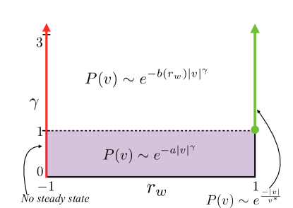
Figure 6: (color online) Schematic diagram summarizing the results obtained in paper. The parameters $r_{w}\in[-1,1]$ is the coefficient of restitution of wall-particle collisions and $\gamma$ characterizes the noise distribution [see Eq. (3)]. When $r_{w}=-1$, the system does not reach a time independent steady state. When $r_{w}=1$, $P(v)$ is universal when $\gamma\geq 1$, and has the same asymptotic behavior as the noise distribution when $\gamma<1$. When the driving is dissipative ($|r_{w}|<1$), $P(v)$ has the same asymptotic behavior as the noise distribution for $\gamma<1$. When $\gamma\geq 1$, the coefficient in the exponential gets modified.

These results generalize the results in Ref. Prasad et al. (2013), where it was shown that for dissipative driving that when the noise distribution is gaussian or Cauchy, the tails of the velocity distribution are similar to that of the noise distribution. The results are also consistent with the intuitive understanding that the tails of velocity distribution are bounded from below by the noise distribution. This is because the tails are populated by particles that have been recently driven and then do not undergo any collision. We expect that more complicated kernels of collision will not change the result. This could be the reason why many of the experimental results Blair and Kudrolli (2001) see non-universal behavior. However, there are experiments that see universal behavior Losert et al. (1999); Rouyer and Menon (2000). In these experiments the $P(v)$ is measured in directions perpendicular to the driving direction. It may be that the details of the driving are lost when energy is transferred to other directions. Transferring energy in other directions ensures that collisions cannot be ignored, unlike the case of one-component Maxwell gas studied in this paper. The two component Maxwell model is a good starting point to answer this question. Methods developed in the paper will be useful to analyze the same. This is a promising area for future study.