Effect of Magnetic Field and Rashba Spin-Orbit Interaction on the Josephson Tunneling between Superconducting Nanowires

Abstract

We calculate the Josephson current between two one-dimensional (1D) nanowires oriented along $x$ with proximity induced $s$-wave superconducting pairing and separated by a narrow dielectric barrier in the presence of both Rashba spin-orbit interaction (SOI) characterized by strength $\alpha$ and Zeeman fields ($h$ along $\hat{z}$ and ${\bf B}$ in the $x-y$ plane). We formulate a general method for computing the Andreev bound states energy which allows us to obtain analytical expressions for the energy of these states in several asymptotic cases. We find that in the absence of the magnetic fields the energy gap between the Andreev bound states decreases with increasing Rashba SOI constant leading eventually to touching of the levels. In the absence of Rashba SOI, the Andreev bound states depend on the magnetic fields and display oscillatory behavior with orientational angle of B leading to magneto-Josephson effect. We also present analytic expressions for the dc Josephson current charting out their dependence on ${\bf B}$, $h$, and $\alpha$. We demonstrate the existence of finite spin-Josephson current in these junctions in the presence of external magnetic fields and provide analytic expressions for its dependence on $\alpha$, $\bf B$ and $h$. Finally, we study the AC Josephson effect in the presence of the SOI (for $|{\bf B}|=h=0$) and an external radiation and show that the width of the resulting Shapiro steps in such a system can be tuned by varying $\alpha$. We discuss experiments which can test our theoretical results.

I Introduction

A recent idea on possible application of topological superconductors to quantum information processing has attracted both theoretical and experimental interest kitaev03 ; nssf08 . According to this idea, a quantum information unit, qubit, can be formed and propagated by means of Majorana mode (see, for e.g., Ref. alicea12, ), localized at the end of a one-dimensional (1D) chain hosting a topological superconductor mzfp12 ; sen1 . Recent investigations suggest several detection mechanisms of such a Majorana mode mzfp12 ; sen1 ; ksy04 ; drmo12 ; rlf12 ; dyhl12 ; cfgd13 ; fhmj13 such as an existence of a central peak in the tunneling current through a topological superconductor (S)- normal metal (N)junction and fractional period of the Josephson current in S-N-S junctions. Most recently experimental systems involving 1D semiconductor wire has been shown to host such modes; the mechanism of the appearance of such modes arise from the combination of strong SOI, proximity-induced superconducting gap, chemical potential and applied Zeeman field in these wires lsd10 ; oro10 . Two Majorana modes in the Josephson junction, formed between two topological insulator edges or one-dimensional superconducting nanowires separated by barrier, hybridize resulting in splitting of the zero energy modes. This splitting energy depends not only on the phase difference of the two superconductors but also on the relative direction of the spin polarization at the two side of the junction.

The oscillations of a Josephson current between two such superconductors separated by insulator or metal as a function of their phase difference, with $4\pi$ periodicity instead of a conventional $2\pi$ periodicity due to hybridization of Majorana states was predicted by Kitaev kitaev01 for a idealized model of an 1D spinless p-wave superconductor. Following this, Kwon et al. ksy04 proposed that the similar effect can be observed between quasi-1D or 2D unconventional superconducting tunnel barrier junctions where the superconductors are separated by an insulating region, usually modeled by a delta function potential barrier. These systems did not have SOI or Zeeman field; Majorana-like modes appeared in such systems from the unconventional nature of the pairing potential. Further it was realized in Ref. ksy04, that a signature of the fractional Josephson effect constitutes in having a halved Josephson frequency, $\omega_{J}=eV/\hbar$, in the presence of a DC voltage $V$ applied across the junction. These effects have been interpreted in terms of the Josephson current being carried by electrons rather than Cooper pairs ksy04 . Further, it was shown that a fractional Josephson effect may be realized at topological insulator edge fk08 ; fk09 . This prediction has later been extended to different systems bhm11 ; jpar11 ; spa12 ; pn12 ; ojanen13 ; scpa13 ; lmay14 ; clgt15 .

Recent activities have established that a topological insulator with proximity-induced coupling to a s-wave superconductor exhibits a superconductivity-magnetism duality nab08 ; jpar11 ; jpar13 ; kss12 ; bphs13 ; pjpa13 , revealing the fractional periodicity not only with superconducting phase difference but also with the orientation of Zeeman magnetic field. In this case, the magnetic field on one side of the junction rotates in the plane normal to the direction of an effective magnetic field of the SOI; consequently, the Majorana-mediated Josephson current reverses sign after $2\pi$ rotation of the magnetic field orientation and reveals an unconventional $4\pi$ periodic magneto-Josephson oscillation in response to variation of the magnetic field orientation in a topological insulator edge jpar11 ; kss12 . Furthermore, a dissipationless fractional Josephson effect mediated by with $8\pi$ periodicity has been also predicted zk14 at the edge of a quantum spin Hall insulator. The Josephson effect in consisting of topological superconducting (S) and normal (N) regions, has been reported in jpar11 ; kss12 ; jpar13 ; pjpa13 . These works also reveal a signature of Majorana bound states located at S-N edges, producing a fractional Josephson current with $4\pi$ periodicity ksy04 .

These previous works in the field have pointed out the importance of the fractional Josephson and the magneto-Josephson effect at the edge of junction of topological insulators. However, the role of spin-orbit coupling and the external magnetic field have not been investigated for $1$D superconducting junctions in these earlier works. In particular, a theoretical formalism for computation of Andreev bound states which requires an extension of the work of Ref. ksy04, to systems with SOC and Zeeman fields is lacking. The development of such a formalism and a systematic study of its results is the main aim of the present work. To this end, we study the Josephson effect between two 1D nanowires oriented along $x$ with proximity induced $s$-wave superconducting pairing and separated by a narrow dielectric with a Rashba spin-orbit interaction (SOI) of strength $\alpha$ and Zeeman fields ($h$ along $\hat{z}$ and ${\bf B}$ in the $x-y$ plane). A schematic representation of the proposed setup is shown in Fig. 1.

The main results of our study are as follows. First, we develop a general method for computing the Andreev bound states energy in these junctions. Such a method constitutes a generalization of the method of Ref. ksy04, to junctions with Zeeman magnetic fields and spin-orbit coupling. Second, using this method, we obtain analytical expressions for the energy of the Andreev bound states in several asymptotic cases and discuss their implication on the Josephson current. For example, we find that in the absence of the magnetic fields the energy gap between these bound states decreases with increasing Rashba SOI constant leading eventually to level touching while in the absence of Rashba SOI, they display oscillatory behavior with orientational angle of ${\bf B}$. Third, we present analytic expressions for the dc Josephson current charting out their dependence on both ${\bf B}$ and $h$ and the SOI interaction strength. Fourth, we demonstrate the existence of finite spin-Josephson current in these junctions in the presence of external magnetic fields and provide analytic expressions for its dependence on $\alpha$, $\bf B$ and $h$. Finally, we study the AC Josephson effect in the presence of the SOI (for $|{\bf B}|=h=0$) and an external radiation and show that the width of the resulting Shapiro steps in such a system can be tuned by varying $\alpha$. We discuss experiments which can test our theoretical results.

The plan of the rest of the paper is as follows. In Sec. II, we describe the model and present explicit form of Hamiltonian. The hybridization energy of edge states is calculated in Sec. III, where several asymptotic expressions for the Josephson coupling energy are obtained. This is followed by a discussion of the DC Josephson effect in Sec. IV. The AC Josephson effect in these system and the dependence of the Shapiro step on SOI strength is studied in Sec. V. Finally we conclude in Sec. VI. Some details of our calculations are specified in the Appendices.

II Model and formulation of the problem

We consider a junction of two 1D nanowires with proximity induced $s$-wave pairing symmetry in the presence of Rashba spin-orbital interaction and external magnetic fields. The schematic representation of such a junction is shown in Fig. 1 where the proximate superconductors are not shown for clarity.

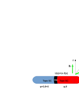
Figure 1: Two s-wave superconductors separated with $\delta$-like dielectric potential under magnetic fields ${\bf h}$ and ${\bf B}$ co-planar and perpendicular to spin-orbit interaction respectively. The bulk s-wave superconductors which induces superconductivity in the wires are not shown for clarity.

In what follows we assume the pairing is induced by two proximate $s$-wave superconductors which leads to effective pairing potentials $\Delta_{1}$ and $\Delta_{2}$ in the two wires. The Hamiltonian for such a system reads

$$\hat{H}=\hat{H}_{SC}+\hat{H}_{R},$$ (1)

where $\hat{H}_{SC}$ is Hamiltonian of the nanowire in the presence of external magnetic fields and $\hat{H}_{R}$ represents Rashba SOI. The former term is given by

$$\hat{H}_{SC} = \int dx\Big{\{}\sum_{\sigma,\sigma^{\prime}}\psi_{\sigma}^{{\dagger}}(x)\Big{(}[\xi_{\hat{k}}+U(x)]\sigma_{0}+h\sigma_{z}$$ (2)

$$+B\{[\sigma_{x}\cos\phi_{1}+\sigma_{y}\sin\phi_{1}]\theta(-x)+[\sigma_{x}\cos\phi_{2}$$

$$+\sigma_{y}\sin\phi_{2}]\theta(x)\}\Big{)}\psi_{\sigma^{\prime}}(x)$$

$$+(\Delta_{1}\theta(-x)+\Delta_{2}\theta(x))\psi_{\uparrow}^{{\dagger}}(x)\psi_{\downarrow}^{{\dagger}}(x)+{\rm h.c.}\Big{\}},$$

where $\xi_{\hat{k}}=\epsilon\left(\frac{\hbar}{i}\frac{\partial}{\partial x}\right)-\epsilon_{F}$ denotes the electron kinetic energy as measured from the Fermi energy $\epsilon_{F}$, $\psi_{\sigma}(x)$ is the electron annihilation operator, $h$ and ${\bf B}$ are external Zeeman magnetic fields in $z$ direction and in the $x-y$ plane respectively, $\theta(x)$ is the Heaviside step function, and $\sigma_{x,y,z}$ and $\sigma_{0}$ denote Pauli and identity matrices respectively in spin space. Note that the magnetic field ${\bf B}$ forms an angle $\phi$ with wire which can be tuned externally. In what follows, we choose ${\bf B}$ in the left side of the junction to be aligned along the wire ($\phi_{1}=0$) while in the right side it is chosen to make an angle $\phi$ with it ($\phi_{2}=\phi$). In Eq. (2), the pairing potential $\Delta_{2}$ in the right of the junction is chosen to have a phase difference $\varphi$ compared to its left counterpart: $\Delta_{2}=|\Delta|\exp(i\varphi)$ and $\Delta_{1}=|\Delta|$. The potential barrier $U(x)=U_{0}\delta(x)$ represents the barrier potential between two superconductors located at $x=0$. The Hamiltonian of Rashba SOI can be written as

$$\hat{H}_{R}=\sum_{\sigma,\sigma^{\prime}}\int dx\psi_{\sigma}^{{\dagger}}(x)\alpha\left[v_{x}\sigma_{z}\right]\psi_{\sigma^{\prime}}(x),$$ (3)

where $\alpha$ is the strength of Rashba SOI which is chosen to be the same for both wires. In what follows, we shall look for the localized subgap Andreev bound states with $\epsilon(k)<|\Delta|$ for the Josephson junction of two nanowires described by Eq. (1).

III Andreev bound states, Josephson and magneto-Josephson effects

In this section, we first obtain solution for the Andreev bound states for junction described by Eq. (1). To do this, it is advantageous to use a four component field operator given by

$$\Psi^{{\dagger}}_{a}(x)=\left(\psi_{a,\uparrow,+}^{{\dagger}}(x),\psi_{a,\downarrow,+}^{{\dagger}}(x),\psi_{a,\downarrow,-}(x),\psi_{a,\uparrow,-}(x)\right)$$ (4)

Here the third subscript of the annihilation operator (which we shall designate henceforth as $b$) labels the right- ($b=+$) and the left-moving $(b=-$) quasiparticles respectively while the index $a=R,L$ denotes either right ($R=-$) or left ($L=+$) superconductor. In terms of the field operator given by Eq. (4), the Hamiltonian (Eq. (1)) can be written as $\hat{H}=\sum_{a=R,L}\int dx\Psi^{{\dagger}}_{a}(x)\mathcal{H}_{a}\Psi_{a}(x)$ using the Pauli matrices $\sigma_{i}$ in spin- and $\tau_{i}$ in particle-hole spaces. From Eqs. (1) and (2), we find

$$\mathcal{H}_{R}=\xi_{k,b}\tau_{z}\sigma_{0}+h\tau_{0}\sigma_{z}-ik\alpha\tau_{z}\sigma_{z}$$ (5)

$$+B\tau_{z}\left(\sigma_{x}\cos\phi+\sigma_{y}\sin\phi\right)+|\Delta|(\tau_{x}\cos\varphi-\tau_{y}\sin\varphi)\sigma_{z},$$

and ${\mathcal{H}}_{L}={\mathcal{H}}_{R}(\phi=0;\varphi=0)$. In Eq. (5), the energy spectrum of the electrons are linearized around the positive and negative Fermi momenta leading to $\xi_{k,b}=bv_{F}\left(-i\frac{\partial}{\partial x}-k_{F}\right)$, where $v_{F}$ is the Fermi velocity. Note that the Hamiltonians $\mathcal{H}_{R,L}$ acquires a magnetism-superconductivity duality nab08 ; jpar13 in the absence of the kinetic term, implying that it becomes invariant under the transformation $\{\Delta,\epsilon_{F},\varphi,\tau_{i}\}\to\{B,h,-\phi,\sigma_{i}\}$. The existence of a magneto-Josephson effect in a topological insulator is known to be a result of this duality jpar13 . We shall see that for the system we study, the magneto-Josephson effect takes place even in the presence of the additional quadratic kinetic energy term of the electrons.

The energy spectrum of quasi-particles in a bulk superconductor in the presence of SOI and external magnetic fields and its expression for different asymptotic is calculated in Appendix A. Note that in our case, all energies are measured from the Fermi energy; thus the condition for realization of a topological superconducting phase with effective $p$-wave pairing is $|\Delta|^{2}>B^{2}+h^{2}$, jpar13 . However, the existence of such a topological phase requires strong $B$ or $h$ and SO interaction so that only the electron band of a single spin species remains below the Fermi surface. In what follows we shall focus on the other regime where the bands of both spin species are below the Fermi surface and the superconductivity is still s-wave.

The Bogolyubov-de Gennes (BdG) equations for the superconductors in the right- and left parts of the barrier are written as

$$\mathcal{H}_{a}\mathbf{\eta}_{a}(x)=E\mathbf{\eta}_{a}(x),\quad a=R,L$$ (6)

where $\eta_{a}(x)$ denotes the BdG wave function. For a barrier modeled by the delta function potential $U(x)=U_{0}\delta(x)$, they satisfy the boundary condition

$$\mathbf{\eta}_{L}(0)=\mathbf{\eta}_{R}(0),\qquad\qquad\partial_{x}\mathbf{\eta}_{R}-\partial_{x}\mathbf{\eta}_{L}=k_{F}Z\mathbf{\eta}(0),$$ (7)

where $Z=2mU_{0}/\hbar^{2}k_{F}$ and the transmission coefficient $D$ is expressed through $Z$ as $D=4/(Z^{2}+4)$.

The constructed wave functions $\eta_{a}(x)$ with the boundary conditions 7 yield the energy of the Andreev bound states for our system. We first note that the Rashba SOI splits the energy spectrum shifting it along the momentum axis, and results in four Fermi momenta at $k=\pm k_{F\pm}$ (see, Eqs. (46) and (47)). The contribution to the Andreev bound states comes from momenta around these Fermi points. The external magnetic field splits spin-up and spin-down electrons (see, Eqs. (49) and (50)) even in the absence of SOI, and the amplitudes of the electron wavefunction are redistributed around four Fermi points due to the presence of such a field. Finally, the presence of a barrier between the two superconductors leads to superposition of the right and left moving quasiparticles. Therefore, the BdG wavefunction $\eta_{a}(x)$ can be written, as it is shown in Appendix  B under (59), as a linear superposition of its right and left moving components with coefficients $A_{a}$, $B_{a}$, $C_{a}$, and $D_{a}$ around each Fermi momentum and with two different spins.

Substituting the wave functions (59) into the boundary conditions (7) one gets eight linear homogeneous equations for $A_{a}$, $B_{a}$, $C_{a}$, and $D_{a}$ with $a=\pm$ which can be represented in terms of a $8\times 8$ matrix $\Lambda$ and a column vector $\Phi=(A_{a},B_{a},C_{a},D_{a})^{T}$ as $\Lambda\Phi=0$. The details of this procedure is charted out in Appendix  B; here, we simply note that, as shown in App. A, the quantities $F_{\sigma\sigma^{\prime}}$ which are determinants of selected blocks of the matrix $\Lambda$ (Eqs. 82 and 92), plays a crucial role in these computations. The energy of the Andreev bound states can then be obtained from ${\rm Det}\Lambda=0$ and thus depend on $F_{\sigma\sigma^{\prime}}$. We note that since the momentum splitting $k_{+}-k_{-}$ vanishes in the absence of SOI and magnetic field; in this limit, either $A_{a}+C_{a}\to A_{a}$ and $B_{a}+D_{a}\to B_{a}$ or both $C_{a}$ and $D_{a}$ vanish. The elements of four columns of the $8\times 8$ determinant, depending on $k_{+}$ become equal to other four column elements as $k_{+}=k_{-}$, and the determinant $\Lambda$ vanishes as $\alpha\to 0$ and $B,h\to 0$.

Andreev bound states at $\alpha=|{\bf B}|=h=0$: In this limit, the Andreev bound states are determined using $4\times 4$ determinant written for electron and hole pairs with opposite spins ksy04 . The details of the calculation is given in C. In order to get the explicit expressions for the wave functions $\eta_{a,\sigma,b}$ and $\eta_{a,{\bar{\sigma}},b}^{\ast}$ we write Eq. (6) for finite $B$, $h$ and $\alpha$ as

$$(E+iabv_{F}k+iab\alpha k-h)\eta_{a,\uparrow,b}-Be^{-i\phi_{a}}\eta_{a,\downarrow,b}$$

$$-\Delta_{a}\eta^{\ast}_{a,\downarrow,\bar{b}}=0$$ (8)

$$(E+iabv_{F}k-iab\alpha k+h)\eta_{a,\downarrow,b}-Be^{i\phi_{a}}\eta_{a,\uparrow,b}$$

$$+\Delta_{a}\eta^{\ast}_{a,\uparrow,\bar{b}}=0$$ (9)

$$(E-iabv_{F}k-iab\alpha k-h)\eta^{\ast}_{a,\downarrow,\bar{b}}+Be^{-i\phi_{a}}\eta^{\ast}_{a,\uparrow,\bar{b}}$$

$$-\Delta_{a}^{\ast}\eta_{a,\uparrow,b}=0$$ (10)

$$(E-iabv_{F}k+iab\alpha k+h)\eta^{\ast}_{a,\uparrow,\bar{b}}+Be^{i\phi_{a}}\eta^{\ast}_{a,\downarrow,\bar{b}}$$

$$+\Delta_{a}^{\ast}\eta_{a,\downarrow,b}=0.$$ (11)

We now use Eq. 11 to compute the Andreev bound state energy at $\alpha=B=h=0$. The details of the calculation is charted out in Appendix  C. As shown in Appendix  C, the contribution to the bound state energy comes only from expression of $F_{\sigma{\bar{\sigma}}}^{\ast}(k)$, and all other ratios vanish. By equating $F_{\sigma{\bar{\sigma}}}^{\ast}(k)$ (Eq. (C)) to zero and using the expressions (43) and (44) for the energy and momentum in this limit, one gets an expression for the bound state energy in consistent with the well-known result abold ; zag1 ; ksy04 ,

$$E_{0}=\pm|\Delta|\sqrt{1-D\sin^{2}\frac{\varphi}{2}}.$$ (12)

Thus our formalism reproduces the earlier known result in the literature in this limit.

Absence of Rashba SOI: In this case, $\alpha=0$ and ${\bf B},h\neq 0$, the main contribution, which depends on the magnetic field orientation, yields the expression (107) with (111) for $F_{\uparrow\uparrow}^{{\dagger}}(k)$ and $F_{\downarrow\downarrow}^{{\dagger}}(k)$. Although the contribution from (106) does depend on the magnetic field, it does not depend on the field orientation $\phi$. A few lines of algebra then leads to the equation for the energy of the Andreev bound states, obtained by equating the sum of (95), (106) and (107) to zero, using (49) and (50) for the energy spectrum and momentum in this limit, given by

$$\left(|\Delta|^{2}-E^{2}_{s}-D|\Delta|^{2}\sin^{2}\frac{\varphi}{2}\right)^{2}+\frac{4E_{s}D|\Delta|^{2}B^{4}\sqrt{B^{2}+h^{2}}}{(h+\sqrt{B^{2}+h^{2}})^{4}}\left(\sin^{2}\frac{(\varphi-\phi)}{2}-\sin^{2}\frac{(\varphi+\phi)}{2}\right)+$$

$$16h\sqrt{B^{2}+h^{2}}D\sin^{2}\frac{\varphi}{2}\left(1-D\sin^{2}\frac{\varphi}{2}\right)\left\{E^{2}_{s}-2\left(1-D\sin^{2}\frac{\varphi}{2}\right)\left[|\Delta|^{2}-4(h^{2}+B^{2})\sin^{2}\frac{\varphi}{2}\right]\right\}=0,$$ (13)

where the second and third terms come from (107) and (106) corresponding to the reflection mechanisms (97) and (98). If we neglect the third contribution, which can be done for $h\ll B$, Eq. (13),can be written

$$E^{2}_{s}-|\Delta|^{2}+D|\Delta|^{2}\sin^{2}\frac{\varphi}{2}\pm|\Delta|\frac{2B^{2}}{(h+\sqrt{B^{2}+h^{2}})^{2}}\sqrt{E_{s}D(B^{2}+h^{2})^{1/2}|\sin\phi|~{}|\sin\varphi|}=0.$$ (14)

We find that Eq. (14) leads to the following features of the Andreev bound states. First, $E_{s}$ decreases with increasing the magnetic field. Second, Eq. 12 is correctly recovered as $B\to 0$.

Eq. (14) can be solved approximately. We replace the energy under square root by its zero-approximation value (12), which yields $E_{s}(B,h)\equiv\pm E_{s}^{M}(B,h)$ with $s=\pm$, where

$$E_{s}^{M}(B,h)=\Bigg{\{}|\Delta|^{2}\left(1-D\sin^{2}\frac{\varphi}{2}\right)-s\frac{2|\Delta|^{3/2}B^{2}}{(h+\sqrt{B^{2}+h^{2}})^{2}}\sqrt{D\sqrt{(B^{2}+h^{2})\left(1-D\sin^{2}\frac{\varphi}{2}\right)}~{}|\sin\phi||\sin\varphi|}~{}\Bigg{\}}^{1/2}$$ (15)

The second term in the bracket of Eq. (15)depends on the magnetic field as $\sim\sqrt{B}$ for $B\gg h$. We note here that $E_{s}(B,h)$ oscillates both with the superconducting phase difference $\varphi$ and the angle orientation $\phi$ of ${\bf B}$ with a period $2\pi$ as shown in Fig. 2. Note that all parameters in the figures presented below are dimensionless ones in the scale of $|\Delta|$, i.e. $B\to B/|\Delta|$, $h\to h/|\Delta|$, $E\to E/|\Delta|$. At $B=0$, Eq. 12 is recovered for $s$-wave superconducting junction and the Andreev bound state energy oscillates with $2\pi$ periodicity (see, Fig. 2a) for barrier transparency $D<1$. The electron-like and hole-like energy branches corresponding to $\pm E_{s}^{M}(B,h)$, touch each other at maximal transmission when $D=1$, creating a zero-energy state at the center of the Brillouin zone. The variation of $B$ and $h$ changes a character of $\varphi$- and $\theta$-dependencies of $E_{s}^{M}$. Note that since the gap between them vanishes at $\varphi=\pi/2$, it might be possible to have a $4\pi$ periodic component of the Josephson current in case of Landau-Zener transitions with a finite transmission probability between two states. This case will be investigated somewhere else.

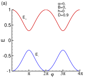
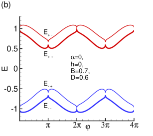
Figure 2: Dependence of the branches energy, given by Eq. (15), on the order parameter phase difference at $\phi=0.5$ and (a) $B=h=0$, $D=0.9$; (b) $h=0.1$, $B=0.9$, $D=0.3$.

Absence of in-plane Zeeman field: Next, we consider the Andreev bound states for $|{\bf B}|=0$, but $\alpha,h\neq 0$. We find that Eqs. (8)- (11) in this case link only $\eta_{a,\sigma,b}$ and $\eta^{\ast}_{a,{\bar{\sigma}},{\bar{b}}}$ and are hence greatly simplified. A few lines of algebra shows that the Andreev bound states energy in this case can be expressed as

$$\left[v_{F}^{2}k^{2}-D\sin^{2}\frac{\varphi}{2}\right]^{2}+$$

$$F_{\uparrow,\downarrow}^{\ast}(k_{+})F_{\downarrow,\uparrow}^{\ast}(k_{-})-F_{\uparrow,\downarrow}^{\ast}(k_{-})F_{\downarrow,\uparrow}^{\ast}(k_{+})=0.$$ (16)

The expression for $F_{\uparrow,\downarrow}^{\ast}(k)$ in this limit is calculated in Appendix C and is given by Eq. (105). The expression for $F_{\downarrow,\uparrow}^{\ast}(k)$ at ${\bf B}=0$ is obtained from Eq. (105) by replacing $\alpha\to-\alpha$ and $h\to-h$. Below we will study two asymptotic solutions of Eq. (16) at $h=0$, $\alpha\neq 0$ and $\alpha=0$, $h\neq 0$. In the former case, Eq. (16) with (105) yields the following equation

$$\left(|\Delta|^{2}-E^{2}-|\Delta|^{2}D\sin^{2}\frac{\varphi}{2}\right)^{2}-$$

$$E^{2}\frac{16v_{F}^{2}\alpha^{2}}{(v_{F}^{2}-\alpha^{2})^{2}}\left(|\Delta|^{2}-E^{2}-|\Delta|^{2}D\sin^{2}\frac{\varphi}{2}\right)D\sin^{2}\frac{\varphi}{2}-$$

$$E^{4}\frac{16v_{F}^{2}\alpha^{2}}{(v_{F}^{2}-\alpha^{2})^{2}}D^{2}\sin^{4}\frac{\varphi}{2}=0.\hskip 14.22636pt$$ (17)

Solution of this equation provides a simple expression for the Josephson energy

$$E_{s}=\pm|\Delta|\left\{\frac{1-D\sin^{2}\frac{\varphi}{2}}{1-\frac{s~{}4v_{F}\alpha}{(v_{F}+s~{}\alpha)^{2}}D\sin^{2}\frac{\varphi}{2}}\right\}^{1/2}\equiv\pm E_{s}^{SOI},$$ (18)

where the sign $\pm$ in the front of the expression signifies an electron and hole energies, whereas the sign $s=\pm$ characterizes Rashba splitting of the electron and hole states. This expression shows that $E_{s}$ depends nonlinearly on the SOI coupling constant $\alpha$. We note that Eq. 12 is once again recovered as $\alpha\to 0$. According to (18), $E$ oscillates still with $2\pi$ period for $D<1$ and $\tilde{\alpha}=\alpha/v_{F}\ll 1$, which is presented in Fig. 3(a) at $\alpha=0.1$ and $D=0.6$. Possible solutions for the energy spectrum according to the expression (18) as a function of the order parameter phase difference at $\alpha=0.205$ and $D=1$ is presented in Fig. 3(b). It shows touching of all four branches at $\varphi=\pi$. The electron- and hole energy branches approach each other faster for non-zero SOI.

The dependence of the $E_{+-}^{SOI}$ energy branches on the order parameter phase difference $\varphi$ at fixed transmission coefficient $D$ and different values of the SOI strength $\alpha$, is presented in the left panel of Fig. 4(a). In Fig. 4(b), we present the dependence of the Andreev bound state energies on $D$ for fixed $\alpha$. We note that both the branches approach zero as $\alpha$ or $D$ is varied.

Absence of $B$ and $\alpha$: Next, we consider the case $|{\bf B}|,\alpha=0$ but $h\neq 0$. In this case, Eq. (16) reduces to

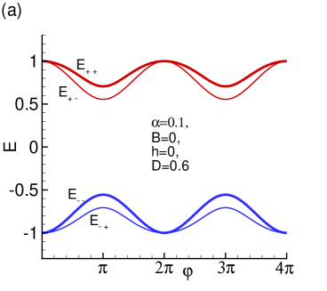
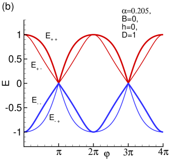
Figure 3: Possible solutions for the branch’s energy spectrum according to the expression (18) as a function of the order parameter phase difference at (a) $\alpha=0.1$ and $D=0.6$, and (b) $\alpha=0.205$ and $D=1$.

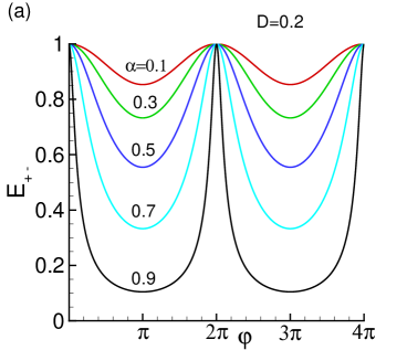
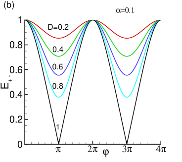
Figure 4: Dependence of the branch’s energy on the order parameter phases difference at (a) $D=0.2$ and different values of the SOI strength, and (b) $\alpha=0.1$ and different values of the transmission coefficient $D$.

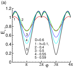
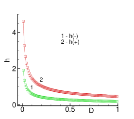
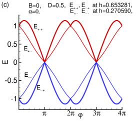
Figure 5: (a) Dependence of the spin-up particle branch’s energy on $\varphi$ at different $\tilde{h}$. Amplitude of the energy oscillation increases with $\tilde{h}$; (b) Mutual optimal values of $\tilde{h}$ and $D$ at which electron- and hole-energy branches are crossed, creating a zero-energy mode; (c) The Andreev bound state energies $E_{h\pm}$ touches at particular values of $D=0.5$ and $\tilde{h}=0.653281$ (thin curves), and of $D=0.5$ and $\tilde{h}=0.270590$ (thick curves) which may make the oscillation period $4\pi$ in the Landau-Zenner sense.

$$\left(|\Delta|^{2}-E^{2}_{h}-D|\Delta|^{2}\sin^{2}\frac{\varphi}{2}\right)^{2}+16E^{2}_{h}h^{2}D\sin^{2}\frac{\varphi}{2}\left(1-D\sin^{2}\frac{\varphi}{2}\right)-$$

$$32h^{2}D\sin^{2}\frac{\varphi}{2}\left(|\Delta|^{2}-4h^{2}D\sin^{2}\frac{\varphi}{2}\right)\left(1-D\sin^{2}\frac{\varphi}{2}\right)^{2}=0,$$ (19)

whose solutions read

$$E_{h}(h)=\pm\sqrt{1-D\sin^{2}\frac{\varphi}{2}}\left\{|\Delta|^{2}-8h^{2}D\sin^{2}\frac{\varphi}{2}+s4h\sqrt{D}\left|\sin\frac{\varphi}{2}\right|\sqrt{|\Delta|^{2}-4h^{2}D\sin^{2}\frac{\varphi}{2}}\right\}^{1/2},$$ (20)

where $s=\pm$. We note that the particle-like and the hole-like branches touch at zero energy; in order to investigate the possible existence of a zero energy mode, which may create a $4\pi$ oscillatory component of the Josephson current in the Landau-Zenner sense, we introduce a dimensionless magnetic field $\tilde{h}=h/|\Delta|$. It is easy to see from Eq. (20) that the condition for the particle and the hole states to cross at a phase difference $\varphi$ is given by

$$\left(\sqrt{1-4\tilde{h}^{2}D\sin^{2}\frac{\varphi}{2}}+2s\tilde{h}\sqrt{D}\left|\sin\frac{\varphi}{2}\right|\right)^{2}-$$

$$8\tilde{h}^{2}D\sin^{2}\frac{\varphi}{2}=0,$$ (21)

which yields

$$\tilde{h}_{s}^{2}=\frac{1}{4D[1+(\sqrt{2}-s)^{2}]\sin^{2}\frac{\varphi}{2}}.$$ (22)

For $\varphi=\pi$, the value of the critical ${\tilde{h}}$ for spin-up ($s=+1$) and spin-down ($s=-1$) states are ${\tilde{h}}_{+}=1/\sqrt{4.6863D}$ and ${\tilde{h}}_{-}=1/\sqrt{27.314D}$, correspondingly. We note here that the bands touch each other at $h=\tilde{h}_{s}$ but do not cross; thus the Andreev states still have $2\pi$ periodic dispersion.

The variation of $E_{h}(h)$ with $\tilde{h}$, the dependence of $\tilde{h}$ on $D$, the touching of the $E_{++}$ and $E_{-+}$ energy branches at $D=0.5$ and $\tilde{h}=0.653281$, and that between $E_{+-}$ and $E_{--}$ energy branches at D=0.5 and $\tilde{h}=0.270590$ are plotted in Fig. 5. In Fig. 5(a), where the dependence of the spin-up particle energy branch on $\varphi$ at different $\tilde{h}$ is presented, we find that the amplitude of the energy oscillation increases with $\tilde{h}$, and additionally, the character of dependence around $\varphi=2\pi$ is changed. In Fig. 5(b) we show the mutual optimal values of $\tilde{h}$ and $D$ at which electron-like and hole-like energy branches touche each other. Finally, the touching of the two branches $E_{++}(h)$ and $E_{-+}(h)$ for $D=0.5$ and $\tilde{h}=0.653281$ is presented in Fig. 5(c). As it was mentioned above, these feature might be responsible for a $4\pi$ periodicity in case of Landau-Zener transitions with a finite transmission probability between two states.

IV Equilibrium Josephson current and spin current

The contribution of the Andreev bound state to the Josephson current can be calculated using to the expression

$$J=\frac{2e}{h}\sum_{n}\frac{\partial E_{n}}{\partial\varphi}~{}f(E_{n}),$$ (23)

where $n$ signifies all states which give a contribution to the current, and $f(E_{n})$ is the Fermi occupation number corresponding to the $n$-th states. We note that since only the Andreev bound states depend explicitly on the phase difference $\varphi$, their expression can be used to determine the DC Josephson current using Eq. (23). In the absence of SOI a contribution to the total equilibrium current gives electron and hole states, each of which is split into two levels due to Zeeman effect

$$J=-\frac{2e}{h}\sum_{s=\pm}\frac{\partial E_{s}^{M}}{\partial\varphi}\tanh\left(\frac{E_{s}^{M}}{2k_{B}T}\right),$$ (24)

where the expression for $E_{s}^{M}$ is given by Eq. (15), and

$$\frac{\partial E_{s}^{M}}{\partial\varphi}=\frac{1}{2E_{s}^{M}}\left[-\frac{D}{2}|\Delta|^{2}\sin\varphi-s\frac{B^{2}|\Delta|^{3/2}\sqrt{D\sqrt{B^{2}+h^{2}}~{}|\sin\phi|}~{}C(\varphi)}{4(1-D\sin^{2}\varphi/2)^{3/4}(h+\sqrt{B^{2}+h^{2}})^{2}\sqrt{|\sin\varphi|}}\right]$$ (25)

with

$$C(\varphi)=\left\{\begin{array}[]{rl}-D\sin^{2}\varphi+4\left(1-D\sin^{2}\frac{\varphi}{2}\right)\cos\varphi&\text{for}\quad 0\leq\varphi<\pi\\ D\sin^{2}\varphi-4\left(1-D\sin^{2}\frac{\varphi}{2}\right)\cos\varphi&\text{for}\quad\pi\leq\varphi<2\pi\end{array}\right.$$ (26)

The current-phase relation at magnetic field $h=0.1$ calculated by using expressions (24), (25) and (26) is presented in Fig. 6. We note, that changes in $h$ does not make an essential effect at $h\leq B$.

Next, we consider the spin-Josephson current which is generated as response to rotation of the magnetic field ${\bf B}=\{B\cos\phi,~{}B\sin\phi,~{}0\}$ in $\{x,~{}y\}$ planejpar13 . As shown in Ref. jpar13, , the spin current can be defined as a derivative of the tunneling energy with respect to the magnetic field orientation $\phi$ and is given by

$$J_{MJ}=\sum_{s=\pm}\frac{\partial E_{s}^{M}}{\partial\phi}\tanh\left(\frac{E_{s}^{M}}{2k_{B}T}\right),$$ (27)

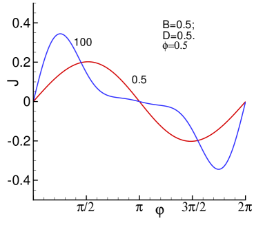
Figure 6: Current-phase relation at magnetic field $h=0.1$ according to the formulas (24)-(26)

Figure 7: Spin current as a function of magnetic field orientation at $D=0.3$, $h=0.1$, $\alpha=0$, $\varphi=0.5$ and two values of magnetic filed $B=0.9$ (curve 1) and $B=2$ (curve 2). Calculations are done according to the formulas (27), (28) and (15).

where

$$\frac{\partial E_{s}^{M}}{\partial\phi}=-sl\frac{B^{2}|\Delta|^{3/2}\sqrt{D\sqrt{(B^{2}+h^{2})(1-D\sin^{2}\varphi/2)}~{}|\sin\varphi|}~{}\cos\phi}{2E_{s}^{M}(h+\sqrt{B^{2}+h^{2}})^{2}\sqrt{|\sin\phi|}},$$ (28)

with $l=1$ for $0\leq\phi<\pi$ and $l=-1$ for $\pi\leq\phi<2\pi$. As it is seen from formulas (25) and (28), the product $E_{s}^{M}\frac{\partial E_{s}^{M}}{\partial\varphi}$ increases with $B$ at $B\gg h$ as $\sqrt{B}$. Instead in the opposite limit when $B\ll h$ this product decreases with increasing $h$ as $\sim B^{2}/h^{3/2}$. On the other hand, in the high temperature limit, when $2k_{B}T\gg E_{s}^{M}$, one can expand $\tan x$ function for small argument $x\ll 1$ as $\tan x\sim x$. Therefore, the amplitude of the supercurrent $J$, given by Eq. (25), and of the spin current $J_{MJ}$, given by Eq. (28), will depend on the magnetic field exactly in the same form as described above for two limiting cases. The change of $h-$direction can rotate the direction of spin current. Spin current as a function of magnetic field orientation at two values of magnetic filed $B=0.9$ and $B=2$ is shown in Fig. 7. Calculations are done according to the formulas (27), (28) and (15).

The Josephson current in other limiting case when $B=h=0$ and $\alpha\neq 0$ is calculated by replacing $E_{s}^{M}$ with $E_{s}^{SOI}$ given by (18) in the expression (24)

$$J=\frac{e|\Delta|}{2h}\sum_{s=\pm}\frac{D\left(1-s\frac{4v_{F}\alpha}{(v_{F}+s\alpha)^{2}}\right)~{}\sin\varphi}{\left[1-s\frac{4v_{F}\alpha}{(v_{F}+s\alpha)^{2}}D\sin^{2}\frac{\varphi}{2}\right]\sqrt{\left(1-D\sin^{2}\frac{\varphi}{2}\right)\left[1-s\frac{4v_{F}\alpha}{(v_{F}+s\alpha)^{2}}D\sin^{2}\frac{\varphi}{2}\right]}}\tanh\left(\frac{E_{s}^{SOI}}{2k_{B}T}\right).$$ (29)

The corresponding plots demonstrated a strong variation of current-phase relation with parameter of spin-orbital coupling $\alpha$ are presented in Fig. 8. The figure demonstrates a crucial breaking of the sinusoidal current-phase relation with increase in spin-orbital coupling. It shows a singular behavior at small $\varphi$.

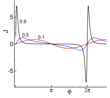
Figure 8: Transformation of current-phase relation with parameter of spin-orbital coupling $\alpha$ at $D=0.5$ (formula (29)). Numbers show the values of parameter spin-orbital coupling.

V AC Josephson Effect

In this section, we compute the AC Josephson effect for the tunnel junctions mentioned above. If there is the voltage in Josephson junction $V(t)=V_{0}+A\cos{\omega t}$, then from Josephson relation $\dot{\varphi}=2eV/\hbar$ we get

$$\varphi(t) = (2e/\hbar)[\varphi_{0}+V_{0}t+\frac{A}{\omega}\sin{\omega t}],$$ (30)

We shall now use this relation to obtain the Shapiro step width for $B=h=0$ and demonstrate that the step-width depends on the strength of the spin-orbit coupling. To do this we first consider the case $\alpha=0$ for which $I_{J}[\phi]$ is given at $T=0$ by

$$I_{S}=\frac{e\Delta}{4\hbar}\frac{D\sin\varphi(t)}{\sqrt{1-(D/2)(1-\cos\varphi(t))/2}}$$ (31)

Substituting Eq. (30) into Eq. (31), one gets

$$\ I_{S}=\frac{e\Delta}{2\hbar}\frac{D\sin({\varphi_{0}+2eV_{0}t/\hbar+\frac{A}{\omega}\sin{\omega t}})}{\sqrt{1-D(1-\cos({\varphi_{0}+2eV_{0}t/\hbar+\frac{A}{\omega}\sin{\omega t}}))/2}}$$ (32)

Using the identity

$$\Im\ e^{i(\varphi_{0}+2eV_{0}t/\hbar+\frac{A}{\omega}\sin{\omega t})}\\ =\Im\sum_{n}J_{n}\left(\frac{A}{\omega}\right)e^{i(\varphi_{0}+t(2eV_{0}/\hbar+n\omega))}$$ (33)

where $\Im$ means imaginary part, $n$ is an integer and $J_{n}$ denotes Bessel function of the first kind, one gets

$$I_{S}=\frac{e\Delta}{2\hbar}\frac{D\Im\sum_{n}J_{n}\left(\frac{A}{\omega}\right)e^{i(\varphi_{0}+t(2eV_{0}/\hbar+n\omega))})}{\sqrt{1-D[1-\Re{\sum_{n}J_{n}\left(\frac{A}{\omega}\right)e^{i(\varphi_{0}+t(2eV_{0}/\hbar+n\omega))}}]/2}}$$ (34)

Here $\Re$ means the real part.

The Shapiro steps thus occur when $2eV_{0}/\hbar=-n_{0}\omega$ for integer $n_{0}$; at these values of the applied radiation frequency, the AC component of the supercurrent vanishes leading to an extra contribution to the dc current in the circuit. The magnitude of the extra DC current from $I_{s}$ can be read off from Eq. (34) as

$$I_{S}^{\rm DC}=\frac{e\Delta}{2\hbar}\frac{D\sin\varphi_{0}J_{n_{0}}\left(\frac{A}{\omega}\right)}{\sqrt{1-D[1-J_{n_{0}}\left(\frac{A}{\omega}\right)\cos(\varphi_{0})]/2}}$$ (35)

From Eq. (35), we find that both the Shapiro step width and the position of maxima/minima of $I_{S}$ depends on $D$. Let us assume that the maxima and minima occur at $\pm\varphi_{0}^{n_{0}}(\omega)$. Note that $\varphi_{0}^{n_{0}}(\omega)$ can be obtained from the solution of $\partial I_{S}/\partial\phi_{0}=0$ and equals $\pm\pi/2$ for $D\ll 1$. In terms of $\varphi_{0}^{n_{0}}(\omega)\equiv\varphi_{0}^{n}$, one obtains the step width as

$$\ \Delta I_{S}=I_{S}^{\rm max}-I_{S}^{\rm min}=\\ \frac{e\Delta}{\hbar}\frac{D\sin(\varphi_{0}^{n})J_{n0}\left(\frac{A}{\omega}\right)}{\sqrt{1-D[1-J_{n_{0}}\left(\frac{A}{\omega}\right)\cos(\varphi_{0}^{n})]/2}}$$ (36)

which clearly shows the $D$ dependence of the step-width.

One can now carry out a similar analysis for the case where $B=h=0$ and $\alpha\neq 0$ (Eq. (18)). Starting from Eq. (23), the AC Josephson current at $T=0$ can be obtained as

$$I_{S}^{\alpha}=\frac{e\Delta}{4\hbar}\\ \sum_{s=\pm}\frac{D(1-\eta_{s})\sin\varphi(t)}{\left[1-\eta_{s}D(1-\cos\varphi(t))/2\right]^{3/2}\left[1-D(1-\cos\varphi(t))/2\right]^{1/2}}$$ (37)

where $\varphi(t)=\varphi_{0}+2eV_{0}t/\hbar+\frac{A}{\omega}\sin{\omega t}$ and $\eta_{s}=4s\alpha v_{F}/(v_{F}+\alpha s)^{2}$. Similar straightforward algebra, as carried out earlier in this section, leads to steps at $n_{0}\omega=-2eV_{0}/\hbar$ with

$$I_{\rm DC}^{\alpha}=\frac{e\Delta DJ_{n_{0}}(\omega)\sin\varphi_{0}}{4\hbar\left[1-D(1-J_{n_{0}}(\omega)\cos\varphi_{0})/2\right]^{1/2}}\sum_{s=\pm}\frac{(1-\eta_{s})}{\left[1-\eta_{s}D(1-J_{n_{0}}(\omega)\cos\varphi_{0})/2\right]^{3/2}}$$ (38)

As before, the minimum and maximum of the DC component of the occurs at $\pm\varphi_{0}^{n_{0}\alpha}(\omega)$ which can be obtained as the solution of $\partial I_{DC}^{\alpha}/\partial\varphi=0$. The step width can thus be expressed in terms of $\varphi_{0}^{n_{0}\alpha}(\omega)\equiv\varphi_{0}^{n_{0}\alpha}$ as

$$\Delta I^{\alpha}=\frac{e\Delta DJ_{n_{0}}(\omega)\sin\varphi_{0}^{n_{0}\alpha}}{2\hbar\left[1-D(1-J_{n_{0}}(\omega)\cos\varphi_{0}^{n_{0}\alpha})/2\right]^{1/2}}\\ \sum_{s=\pm}\frac{(1-\eta_{s})}{\left[1-\eta_{s}D(1-J_{n_{0}}(\omega)\cos\varphi_{0}^{n_{0}\alpha})/2\right]^{3/2}}$$ (39)

Thus we find the step width depends on the magnitude of the spin-orbit coupling. Indeed, Fig. 9(a) demonstrates this effect of transparency and spin-orbital coupling on the $\varphi$-dependence of the Shapiro step width according to formula (39). We also note that for $D\ll 1$, the maxima and minima of the DC current occur for $\varphi_{0}^{n_{0}\alpha}\simeq\pm\pi/2$ and Eq. (39) simplifies to yield

$$\Delta I^{\alpha}(D\ll 1) \simeq \frac{e\Delta D}{2\hbar}J_{n_{0}}(\omega)\left(2-\eta_{+}-\eta_{-}\right)$$ (40)

For small $\tilde{\alpha}=\alpha/v_{F}$, it is easy to see by expanding $\eta_{\pm}$ in power of $\tilde{\alpha}$, that

$$\Delta I^{\alpha}(D\ll 1;\tilde{\alpha}\ll 1) \simeq \frac{e\Delta D}{\hbar}J_{n_{0}}(\omega)\left(1+4\tilde{\alpha}^{2}+...\right)$$

which demonstrates the dependence of step width on the SO coupling $\alpha$.

Comparison of these three plots according to Eqs. (39), (40) and (V) is presented in Fig. 9(b). As we can see, the results of approximations (40) and (V) demonstrate more sharper increasing of Shapiro step width with $\alpha$ in compare with formula (39). It’s clear that the difference disappears in the limit $D\rightarrow 0$. The obtained dependence of the SS width on the spin-orbit coupling may be used for the experimental estimation of its value.

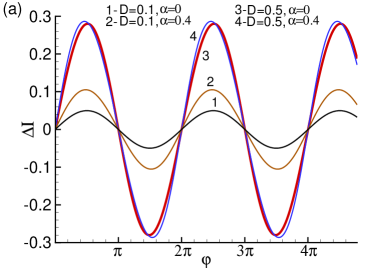
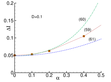
Figure 9: (a) Effect of transparency and spin-orbital coupling on the $\varphi$-dependence of the Shapiro step width according to the formula (39); (b) Demonstration of $\alpha$-dependence of Shapiro step width in different approximations according to the formulas (39), (40) and (V).

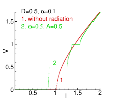
Figure 10: I-V curve at $D=0.5$, $\alpha=0.1$ without radiation (curve 1) and under external radiation (curve 2)

To investigate the effect of SOI on the amplitude dependence of Shapiro step width, we have calculated the I-V curves for the junction under external radiation using equation (37). This result is presented in Fig. 10, where we show the I-V curve of the junction at $D=0.5$, $\alpha=0.1$ under external electromagnetic radiation with frequency $\omega=0.5$ and amplitude $A=0.5$. In this figure we include for comparison the I-V characteristics without radiation also. The I-V curve demonstrates the main Shapiro step at $V=\omega=0.5$ and its harmonics.

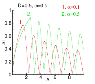
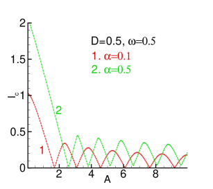
Figure 11: Effect of spin orbital coupling on the amplitude dependence of: (a) Shapiro step width; (b) Critical current.

Fig. 11(a) shows the amplitude dependence of Shapiro step width in case $\alpha=0.5$ (line 1) and $\alpha=0.1$ (line 2) under external radiation with frequency $\omega=0.5$. Calculation is provided for value of transparency $D=0.5$. We see that the value of the SOI parameter has a noticeable effect on the Shapiro step width and its dependence on amplitude of the external radiation. These results of I-V characteristics simulations coincide qualitatively with the conclusion followed from Fig. 9. We see that in case with $\alpha=0.5$ the width of Shapiro step is larger than case $\alpha=0.1$. The similar effect can be seen in amplitude dependence of critical current $I_{c}$, which is shown in Fig. 11(b).

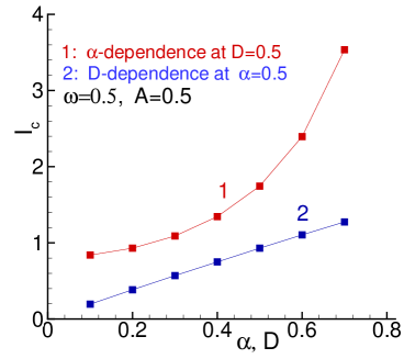
Figure 12: The $\alpha$–dependence of $I_{c}$ for $D=0.5$ and $D$–dependence of $I_{c}$ for $\alpha=0.2$ at $\omega=0.5$, $A=0.5$.

The transparency coefficient $D$ also effects the critical current value. To distinguish and clarify the effect of SOI we have calculated the $\alpha$– and $D$–dependence of $I_{c}$, which is demonstrated in Figures 12 (a) and (b). These results might be used for the comparison with future experimental results.

VI Conclusion

In this paper we study the Josephson current between 1D superconducting nanowires separated by an insulating barrier in the presence of Rashba SOI and the magnetic fields ${\bf B}$ and $h$. The presence of the SOI and Zeeman magnetic fields leads to four distinct Fermi points in each bulk superconductor. Therefore, the study of Josephson effect in these junctions requires construction of an incident quasiparticle wave function which is in a linear superposition state of plane waves around each Fermi points. In our study, we have developed a theoretical method to study Josephson effect in such systems; our work thus constitutes a generalization of analysis of Ref. ksy04, to systems with SOI and Zeeman fields. We have provided analytical results for the Andreev bound states in several asymptotic limits from our analysis, demonstrated the presence of spin-Josephson current in these junctions, and studied the dependence of Shapiro steps on SOI interaction strength $\alpha$ in the presence of external radiation. Moreover, we have demonstrated the existence of magneto-Josephson effect in these systems. We note that although the existence of the magneto-Josephson effect in a topological superconductor has been predicted recently jpar13 ; kss12 ; pjpa13 , the question of whether this effect is observable in superconducting junctions with quadratic electronic dispersion and the absence of SOI was not addressed before. We show in the paper the magneto-Josephson effect takes place even in the absence of SOI.

Experimental verification of our work would require experiments conducted on Josephson junctions in 1D nanowires analogous to ones studied in Ref. rlf12, . We predict that the variation of the angle $\phi$ of the in-plane magnetic field ${\bf B}$ would lead to a spin-Josephson current as shown in Fig. 7. Furthermore, AC Josephson effect measurement in these junction, analogous to those done in Ref. rlf12, , should reveal a quadratic dependence of the Shapiro step-width as a function of $\alpha$ for small $\alpha/v_{F}$ as shown in Fig. 12.

Our work allows for several possible future direction. First, a numerical solution of the condition ${\rm Det}\Lambda=0$ yielding Andreev bound state energies in the regime where ${\bf B},\alpha,h\neq 0$ may lead to a better understanding of the interplay between these parameters to shape the characteristics of the bound state energies. Second, the formalism that we develop here may be extended to regime of strong $\alpha$ and $B$ where the presence of Majorana bound states shapes the characteristics of the Josephson current. This requires a separate analysis since in this case the quasiparticles would originates from two ( and not four Fermi points) and is left as a topic for future study. Third, our formalism may be applied to cases where the superconducting pair-potential is unconventional (for example p-wave); indeed, interplay of such unconventional pair-potentials and SO coupling may lead to additional interesting characteristics in the Josepshon current. We intend to explore these issues in future work.

In conclusion, we have studied Josephson effect in a unction between two 1D nanowires in the presence of SOI and zeeman fields. We have analyzed the Josephson current in these junctions and provided analytical expressions of the Andreev bound states in several limiting cases. We have also demonstrated the presence of magneto-Josephson effect in these junctions and studied the Shapiro step width in AC Josephson effect on the SOI strength. Our theoretical predictions are shown to be verifiable by straightforward experiments on these systems.

Appendix A Energy dispersion for BdG superconductor

The expression ${\rm Det}|\mathcal{H}-E|=0$ for the energy spectrum is written

$$\begin{vmatrix}E_{11},&-Be^{-i\phi},&-\Delta,&0\\ -Be^{i\phi},&E_{22},&0,&\Delta\\ -\Delta^{\ast},&0,&E_{33},&Be^{-i\phi}\\ 0,&\Delta^{\ast},&Be^{i\phi},&E_{44}\end{vmatrix}=0$$

where $E_{11}=E+iabv_{F}k+iab\alpha k-h$, $E_{22}=E+iabv_{F}k-iab\alpha k+h$, $E_{33}=E-iabv_{F}k-iab\alpha k-h$, and $E_{44}=E-iabv_{F}k+iab\alpha k+h$. Calculation of this determinant yields the energy spectrum of a “bulk” $1D$ superconductor

$$\left(E^{2}-v_{F}^{2}k^{2}+\alpha^{2}k^{2}-h^{2}-B^{2}-|\Delta|^{2}\right)^{2}+4\left(Ekv_{F}+h\alpha k\right)^{2}-4|\Delta|^{2}\left(v_{F}^{2}k^{2}+B^{2}+h^{2}\right)=0$$ (42)

This expression contains a linear in energy term, which is a result of an alignment of ${\bf h}$ and the effective magnetic field of the SOI $\propto\alpha k$.

We consider different limiting cases below.

• The case of $\alpha=B=h=0$.

The energy spectrum looks

$$E_{\pm}=\pm\sqrt{|\Delta|^{2}-v_{F}^{2}k^{2}}.$$ (43)

The energy levels of BdG quasi-particles lie in the gap, symmetrical to the Fermi level, with momentum

$$k=\pm\frac{\sqrt{|\Delta|^{2}-E^{2}}}{v_{F}}.$$ (44)

• The case of $B=0$, but $h\neq 0$ and $\alpha\neq 0$.

The energy spectrum (42) in this limiting case is factorized

$$\left[(E+h)^{2}+(v_{F}-\alpha)^{2}k^{2}-|\Delta|^{2}\right]\left[(E-h)^{2}+(v_{F}+\alpha)^{2}k^{2}-|\Delta|^{2}\right]=0.$$ (45)

One gets for the quasi-particles’ energy

$$E_{s,\pm}=sh\pm\sqrt{|\Delta|^{2}-(v_{F}+s\alpha)^{2}k^{2}},$$ (46)

where $s=\pm$. The momenta is expressed as

$$k_{\pm}^{2}=\frac{|\Delta|^{2}-(E\mp h)^{2}}{(v_{F}\pm\alpha)^{2}}.$$ (47)

SOI and/or magnetic field $h$ split both electron and hole levels due to Rashba ’momentum-shifting’ and/or Zeeman effect. The ’Fermi points’ around $+k_{F}$ and $-k_{F}$ are split also due to these effects.

• The limit of $\alpha=0$, and $B\neq 0$, $h\neq 0$.

Expression (42) under these conditions reads

$$\left[\left(E+\sqrt{B^{2}+h^{2}}\right)^{2}+v_{F}^{2}k^{2}-|\Delta|^{2}\right]\left[\left(E-\sqrt{B^{2}+h^{2}}\right)^{2}+v_{F}^{2}k^{2}-|\Delta|^{2}\right]=0,$$ (48)

yielding the following expression for the energy spectrum

$$E^{2}=\left(\sqrt{|\Delta|^{2}-v_{F}^{2}k^{2}}\pm\sqrt{B^{2}+h^{2}}\right)^{2}.$$ (49)

The momenta around the Fermi ’points’ $+k_{F}$ and $-k_{F}$ split also

$$k_{\pm}^{2}=\frac{|\Delta|^{2}-\left(E\mp\sqrt{B^{2}+h^{2}}\right)^{2}}{v_{F}^{2}}.$$ (50)

The expressions for the energy and momentum in the limits of $\alpha=0$, ${\bf B}=0$ but $h\neq 0$ or of $\alpha=0$, $h=0$ but ${\bf B}\neq 0$ are easily obtained from (49) and (50). Note that a topological superconducting gapped phase is realized when $|\Delta|^{2}>B^{2}+h^{2}$ in consistent with Ref.jpar13 .

Appendix B Computation of the Andreev bound states

In this section, we chart out the expression for $\Lambda$. The BdG wavefunction $\eta_{a}(x)$ can be written as a linear superposition of its right and left moving components around each Fermi momentum and with two different spins. Since we look for bound state solutions, the general solution of Eq. (6) with (5) can be written as

$$\mathbf{\eta}_{a}(x)=\sum_{j=\pm}e^{{\rm sgn}(a)k_{j}x}\left[A_{a}^{j}\left(\begin{array}[]{ccc}\eta_{a,\uparrow,+}(k_{j})\\ \eta_{a,\downarrow,+}(k_{j})\\ \eta_{a,\downarrow,-}^{\ast}(k_{j})\\ \eta_{a,\uparrow,-}^{\ast}(k_{j})\end{array}\right)e^{ik_{Fj}x}+B_{a}^{j}\left(\begin{array}[]{ccc}\eta_{a,\uparrow,-}(k_{j})\\ \eta_{a,\downarrow,-}(k_{j})\\ \eta_{a,\downarrow,+}^{\ast}(k_{j})\\ \eta_{a,\uparrow,+}^{\ast}(k_{j})\end{array}\right)e^{-ik_{Fj}x}\right]$$ (59)

where $k_{a}^{-1}$ denotes the localization length of the bound states, and ${\rm sgn}(a)=+(-)$ for $a=L(R)$. Henceforth, we shall rename the coefficients as $A_{a}^{+}\equiv A_{a}$, $A_{a}^{-}\equiv C_{a}$, and $B_{a}^{+}\equiv B_{a}$, $B_{a}^{-}\equiv D_{a}$ for clarity. Substituting the wave functions (59) into the boundary conditions (7) one gets eight linear homogeneous equations for $A_{a}$, $B_{a}$, $C_{a}$, and $D_{a}$ with $a=\pm$ which can be represented in terms of a $8\times 8$ matrix $\Lambda$ and a column vector $\Phi=(A_{a},B_{a},C_{a},D_{a})^{T}$ as $\Lambda\Phi=0$. The energy of the Andreev bound states can then be obtained from ${\rm Det}\Lambda=0$. The expression for the matrix $\Lambda$, obtained from some straightforward algebra, is given by

$$\Lambda = \left(\begin{array}[]{cc}D_{1}&D_{2}\\ D_{3}&D_{4}\end{array}\right)$$ (62)

$$D_{1} = \left(\begin{array}[]{cccc}\eta_{-\uparrow+}(k_{+}),&\eta_{-\uparrow-}(k_{+}),&-\eta_{+\uparrow-}(k_{+}),&-\eta_{+\uparrow+}(k_{+})\\ \eta_{-\downarrow+}(k_{+}),&\eta_{-\downarrow-}(k_{+}),&-\eta_{+\downarrow-}(k_{+}),&-\eta_{+\downarrow+}(k_{+})\\ \eta^{\ast}_{-\downarrow-}(k_{+}),&\eta^{\ast}_{-\downarrow+}(k_{+}),&-\eta^{\ast}_{+\downarrow+}(k_{+}),&-\eta^{\ast}_{+\downarrow-}(k_{+}),\\ \eta^{\ast}_{-\uparrow-}(k_{+}),&\eta^{\ast}_{-\uparrow+}(k_{+}),&-\eta^{\ast}_{+\uparrow+}(k_{+}),&-\eta^{\ast}_{+\uparrow-}(k_{+})\end{array}\right)$$ (67)

$$D_{2} = \left(\begin{array}[]{cccc}\eta_{-\uparrow+}(k_{-}),&\eta_{-\uparrow-}(k_{-}),&-\eta_{+\uparrow-}(k_{-}),&-\eta_{+\uparrow+}(k_{-})\\ \eta_{-\downarrow+}(k_{-}),&\eta_{-\downarrow-}(k_{-}),&-\eta_{+\downarrow-}(k_{-}),&-\eta_{+\downarrow+}(k_{-})\\ \eta^{\ast}_{-\downarrow-}(k_{-}),&\eta^{\ast}_{-\downarrow+}(k_{-}),&-\eta^{\ast}_{+\downarrow+}(k_{-}),&-\eta^{\ast}_{+\downarrow-}(k_{-})\\ \eta^{\ast}_{-\uparrow-}(k_{-}),&\eta^{\ast}_{-\uparrow+}(k_{-}),&-\eta^{\ast}_{+\uparrow+}(k_{-}),&-\eta^{\ast}_{+\uparrow-}(k_{-})\end{array}\right)$$ (72)

$$D_{3} = \left(\begin{array}[]{cccc}C_{--}^{+}\eta_{-\uparrow+}(k_{+}),&-C_{++}^{+}\eta_{-\uparrow-}(k_{+}),&C_{--}^{+}\eta_{+\uparrow-}(k_{+}),&-C_{++}^{+}\eta_{+\uparrow+}(k_{+})\\ C_{--}^{+}\eta_{-\downarrow+}(k_{+}),&-C_{++}^{+}\eta_{-\downarrow-}(k_{+}),&C_{--}^{+}\eta_{+\downarrow-}(k_{+}),&-C_{++}^{+}\eta_{+\downarrow+}(k_{+})\\ C_{--}^{+}\eta^{\ast}_{-\downarrow-}(k_{+}),&-C_{++}^{+}\eta^{\ast}_{-\downarrow+}(k_{+}),&C_{--}^{+}\eta^{\ast}_{+\downarrow+}(k_{+}),&-C_{++}^{+}\eta^{\ast}_{+\downarrow-}(k_{+})\\ C_{--}^{+}\eta^{\ast}_{-\uparrow-}(k_{+}),&-C_{++}^{+}\eta^{\ast}_{-\uparrow+}(k_{+}),&C_{--}^{+}\eta^{\ast}_{+\uparrow+}(k_{+}),&-C_{++}^{+}\eta^{\ast}_{+\uparrow-}(k_{+}),\end{array}\right)$$ (77)

$$D_{4} = \left(\begin{array}[]{cccc}C_{--}^{-}\eta_{-\uparrow+}(k_{-}),&-C_{++}^{-}\eta_{-\uparrow-}(k_{-}),&C_{--}^{-}\eta_{+\uparrow-}(k_{-}),&-C_{++}^{-}\eta_{+\uparrow+}(k_{-})\\ C_{--}^{-}\eta_{-\downarrow-}(k_{-}),&-C_{++}^{-}\eta_{-\downarrow-}(k_{-}),&C_{--}^{-}\eta_{+\downarrow-}(k_{-}),&-C_{++}^{-}\eta_{+\downarrow+}(k_{-})\\ C_{--}^{-}\eta^{\ast}_{-\downarrow-}(k_{-}),&-C_{++}^{-}\eta^{\ast}_{-\downarrow+}(k_{-}),&C_{--}^{-}\eta^{\ast}_{+\downarrow+}(k_{-}),&-C_{++}^{-}\eta^{\ast}_{+\downarrow-}(k_{-})\\ C_{--}^{-}\eta^{\ast}_{-\uparrow-}(k_{-}),&-C_{++}^{-}\eta^{\ast}_{-\uparrow+}(k_{-}),&C_{--}^{-}\eta^{\ast}_{+\uparrow+}(k_{-}),&-C_{++}^{-}\eta^{\ast}_{+\uparrow-}(k_{-})\end{array}\right)$$ (82)

where $C_{\mu\nu}^{\pm}=(ik_{F}+\mu k_{\pm}+\nu k_{F}Z/2)$ and $\nu,\mu$ takes values $\pm 1$.

We note that it is difficult to obtain analytical expression of ${\rm Det}\Lambda$ for general values of $B$, $\alpha$ and $h$. However, the physical content of the several terms in this determinant can be understood as follows. We define the minors of the selected blocks of $\Lambda$ as ${\rm Det}D_{1}={\tilde{F}}^{\ast}_{\uparrow\downarrow}(k_{+})$, ${\rm Det}D_{2}={\tilde{F}}^{\ast}_{\uparrow\downarrow}(k_{-})$, ${\rm Det}D_{3}={\tilde{F}}_{\downarrow\uparrow}(k_{+})$, ${\rm Det}D_{4}={\tilde{F}}^{\ast}_{\downarrow\downarrow}(k_{-})$. Furthermore we define the $4\times 4$ matrices

$$D_{5} = \left(\begin{array}[]{cccc}\eta_{-\uparrow+}(k_{+}),&\eta_{-\uparrow-}(k_{+}),&-\eta_{+\uparrow-}(k_{+}),&-\eta_{+\uparrow+}(k_{+})\\ \eta^{\ast}_{-\uparrow-}(k_{+}),&\eta^{\ast}_{-\uparrow+}(k_{+}),&-\eta^{\ast}_{+\uparrow+}(k_{+}),&-\eta^{\ast}_{+\uparrow-}(k_{+})\\ C_{--}^{+}\eta_{-\uparrow+}(k_{+}),&-C_{++}^{+}\eta_{-\uparrow-}(k_{+}),&C_{--}^{+}\eta_{+\uparrow-}(k_{+}),&-C_{++}^{+}\eta_{+\uparrow+}(k_{+})\\ C_{--}^{+}\eta^{\ast}_{-\uparrow-}(k_{+}),&-C_{++}^{+}\eta^{\ast}_{-\uparrow+}(k_{+}),&C_{--}^{+}\eta^{\ast}_{+\uparrow+}(k_{+}),&-C_{++}^{+}\eta^{\ast}_{+\uparrow-}(k_{+})\end{array}\right)$$ (87)

$$D_{6} = \left(\begin{array}[]{cccc}\eta_{-\downarrow+}(k_{+}),&\eta_{-\downarrow-}(k_{+}),&-\eta_{+\downarrow-}(k_{+}),&-\eta_{+\downarrow+}(k_{+})\\ \eta^{\ast}_{-\downarrow-}(k_{+}),&\eta^{\ast}_{-\downarrow+}(k_{+}),&-\eta^{\ast}_{+\downarrow+}(k_{+}),&-\eta^{\ast}_{+\downarrow-}(k_{+})\\ C_{--}^{+}\eta_{-\downarrow+}(k_{+}),&-C_{++}^{+}\eta_{-\downarrow-}(k_{+}),&C_{--}^{+}\eta_{+\downarrow-}(k_{+}),&-C_{++}^{+}\eta_{+\downarrow+}(k_{+})\\ C_{--}^{+}\eta^{\ast}_{-\downarrow-}(k_{+}),&-C_{++}^{+}\eta^{\ast}_{-\downarrow+}(k_{+}),&C_{--}^{+}\eta^{\ast}_{+\downarrow+}(k_{+}),&-C_{++}^{+}\eta^{\ast}_{+\downarrow-}(k_{+})\end{array}\right)$$ (92)

The determinants of these matrices are denoted by ${\rm Det}D_{5}=F^{\ast}_{\uparrow\uparrow}(k_{+})$ and ${\rm Det}D_{6}=F^{\ast}_{\downarrow\downarrow}(k_{+})$. Similarly one can also construct expressions for $F^{\ast}_{\uparrow\uparrow}(k_{-})$ and $F^{\ast}_{\downarrow\downarrow}(k_{+})$. Note that all these blocks are interpreted to correspond to a definitive physical process as explained in the main text. All of these determinants enter the expressions of the Andreev bound states as discussed in Sec. III of the main text.

Appendix C Andreev bound states at B=0

In this section we look into the expression of Andreev bound states for $|{\bf B}|=0$. The boundary conditions (7) for the wave function (59), written in the absence of the SOI induced momentum splitting yield again eight equations for four coefficients $A_{\pm}$ and $B_{\pm}$; these equations are BdG equations for a s-wave superconductor with spin-dependent eigenfunctions $\eta_{a,\sigma,b}$ and $\eta_{a,{\bar{\sigma}},b}^{\ast}$, where the overline of an index (e.g., ${\bar{\sigma}}$) means an opposite direction or sign. One chooses four equations corresponding to an electron-hole pair with opposite spins. The determinant corresponding to the matrix (defined as $D_{1}$ in Appendix B) in the front of the coefficients $A_{a}$ and $B_{a}$ is calculated to give

$${\tilde{F}}_{\uparrow,\downarrow}^{\ast}=\frac{1}{D^{2}}\eta_{+,\downarrow,+}\eta_{-,\downarrow,-}\eta_{+,\downarrow,-}\eta_{-,\downarrow,+}F^{\ast}_{\uparrow,\downarrow},$$ (93)

where

$$F_{\uparrow,\downarrow}^{\ast}=\left[\frac{\eta^{\ast}_{-,\uparrow,-}}{\eta_{-,\downarrow,+}}-\frac{\eta^{\ast}_{+,\uparrow,-}}{\eta_{+,\downarrow,+}}\right]\left[\frac{\eta^{\ast}_{+,\uparrow,+}}{\eta_{+,\downarrow,-}}-\frac{\eta^{\ast}_{-,\uparrow,+}}{\eta_{-,\downarrow,-}}\right]-$$ (94)

$$(1-D)\left[\frac{\eta^{\ast}_{+,\uparrow,-}}{\eta_{+,\downarrow,+}}-\frac{\eta^{\ast}_{-,\uparrow,+}}{\eta_{-,\downarrow,-}}\right]\left[\frac{\eta^{\ast}_{-,\uparrow,-}}{\eta_{-,\downarrow,+}}-\frac{\eta^{\ast}_{+,\uparrow,+}}{\eta_{+,\downarrow,-}}\right].$$

Equating this determinant to zero one gets a condition to find the energy spectrum ksy04 . Note that the other four equations yields the same expression with only spin being interchanged leading to ${\tilde{F}}_{\downarrow,\uparrow}^{\ast}$. It is easy to see that the condition to determine the Andreev bound state energy in this limit, where $\Lambda$ constitutes two $4\times 4$ blocks, is given by equating

$${\tilde{F}}_{\uparrow,\downarrow}^{\ast}\cdot{\tilde{F}}_{\downarrow,\uparrow}^{\ast}$$ (95)

to zero. Eqs. (8)..(11) allow us to calculate all possible ratios $\eta^{\ast}_{a,\sigma,b}/\eta_{a,{\bar{\sigma}},{\bar{b}}}$, $\eta^{\ast}_{a,\sigma,b}/\eta_{a,\sigma,{\bar{b}}}$, and $\eta_{a,\sigma,b}/\eta_{a,{\bar{\sigma}},b}$, $\eta^{\ast}_{a,\sigma,b}/\eta^{\ast}_{a,{\bar{\sigma}},b}$. Furthermore, we note that only the ratio $\eta^{\ast}_{a,\sigma,b}/\eta_{a,{\bar{\sigma}},{\bar{b}}}$ is non-zero for ${\bf B}=0$. We shall return to this case below.

Next, we note from Eqs. (8)..(11) that the dependencies of these equations on $\phi$ and $\varphi$ are completely removed by transforming the wave function as

$$\eta^{\ast}_{a}(x) \to \left(e^{-i(\varphi-\phi)/2}\eta_{a,\uparrow,\bar{b}}^{\ast}(x),~{}e^{-i(\varphi+\phi/2)}\eta_{a,\downarrow,\bar{b}}^{\ast}(x),\right.$$ (96)

$$\left.~{}e^{i(\varphi+\phi)/2}\eta_{a,\downarrow,b}(x),~{}e^{i(\varphi-\phi)/2}\eta_{a,\uparrow,b}(x)\right).$$

In the transformed basis one has

$$\frac{\eta^{\ast}_{a,\uparrow,b}}{\eta_{a,\uparrow,{\bar{b}}}}\to e^{-i(\varphi-\phi)}\frac{\eta^{\ast}_{a,\uparrow,b}}{\eta_{a,\uparrow,{\bar{b}}}},\quad\frac{\eta^{\ast}_{a,\downarrow,b}}{\eta_{a,\downarrow,{\bar{b}}}}\to e^{-i(\varphi+\phi)}\frac{\eta^{\ast}_{a,\downarrow,b}}{\eta_{a,\downarrow,{\bar{b}}}}$$ (97)

$$\frac{\eta^{\ast}_{a,\uparrow,b}}{\eta_{a,\downarrow,{\bar{b}}}}\to e^{-i\varphi}\frac{\eta^{\ast}_{a,\uparrow,b}}{\eta_{a,\downarrow,{\bar{b}}}},\quad\frac{\eta^{\ast}_{a,\downarrow,b}}{\eta_{a,\uparrow,{\bar{b}}}}\to e^{-i\varphi}\frac{\eta^{\ast}_{a,\downarrow,b}}{\eta_{a,\uparrow,{\bar{b}}}}$$ (98)

$$\frac{\eta^{\ast}_{a,\uparrow,b}}{\eta_{a,\downarrow,b}^{\ast}}\to e^{i\phi}\frac{\eta^{\ast}_{a,\uparrow,b}}{\eta_{a,\downarrow,b}^{\ast}},\quad\frac{\eta_{a,\uparrow,b}}{\eta_{a,\downarrow,b}}\to e^{-i\phi}\frac{\eta_{a,\uparrow,b}}{\eta_{a,\downarrow,b}}.$$ (99)

The different ratios that appear in the left-side of Eqs. 97..99 can be understood as follows. The ratio $\eta^{\ast}_{a,\sigma,b}/\eta_{a,{\bar{\sigma}},{\bar{b}}}$ corresponds to the amplitude of conventional Andreev reflection channel which constitutes reflection of an electron-like quasiparticle to a hole-like quasiparticle with opposite spin on a N-S interface. In contrast, the ratio $\eta^{\ast}_{a,\sigma,b}/\eta_{a,\sigma,{\bar{b}}}$ which is finite only in the presence of SOI and/or magnetic field, represents amplitude of Andreev reflection channel where the electron-like quasiparticle incident on the interface is reflected to a hole-like quasiparticle state with the same spin orientation. Finally, the ratio $\eta_{a,\sigma,b}/\eta_{a,{\bar{\sigma}},}b$ represents a usual reflection channel of an electron-like quasiparticle on the boundary without creation of a Cooper pair in a superconducting part of the junction. Since these ratios enter the expressions of $F_{\sigma\sigma^{\prime}}$, these also represents Andreev and normal reflection processes involving electron-like and hole-like quasiparticles in the opposite ($\sigma^{\prime}=\bar{\sigma}$) and same ($\sigma^{\prime}=\sigma$) spin sector. We note that the ratio of wavefunctions in Eq. (97) depend on both $\phi$ and $\varphi$ while those in Eqs. (98) and (99) depend on either $\varphi$ or $\phi$. This suggests that the ratios (97) and (98) are responsible for the dependence of observable parameters on the order parameter phase difference $\varphi$, whereas the ratios (97) and (99) are responsible for the dependence on the magnetic field orientation angle $\phi$.

The ratios $\eta^{\ast}_{a,\uparrow,{\bar{b}}}/\eta_{a,\downarrow,b}$ and $\eta^{\ast}_{a,\downarrow,{\bar{b}}}/\eta_{a,\uparrow,b}$ are determined from Eqs. (8)-(11) as

$$\frac{\eta^{\ast}_{a,\sigma,\bar{b}}}{\eta_{a,\bar{\sigma},b}} = \pm\frac{1}{\Delta_{a}}\bigg{\{}\frac{M_{\pm}(k)}{2(E\pm iab\alpha k)}$$ (100)

$$-(E+iabv_{F}k\mp iab\alpha k\pm h)\bigg{\}},$$

$$M_{\pm}(k) = (E\pm h)^{2}+(v_{F}k\mp\alpha k)^{2}+B^{2}-|\Delta|^{2},$$ (101)

where the upper (lower) sign $+$ ($-$) corresponds to spin $\sigma=\uparrow$ ($\sigma=\downarrow$). Using Eq. (100), one obtains, after a few lines of algebra, the expressions for $F_{\uparrow,\downarrow}^{\ast}$ and $F_{\downarrow,\uparrow}^{\ast}$ for general ${\bf B}$, $h$ and $\alpha$ as

$$F_{\sigma{\bar{\sigma}}}^{\ast}(k)=\big{\{}\big{[}\alpha kM_{\pm}(k)\pm 2(v_{F}k\mp\alpha k)(E^{2}+\alpha^{2}k^{2})\big{]}^{2}$$

$$-4D|\Delta|^{2}(E^{2}+\alpha^{2}k^{2})^{2}\sin^{2}\frac{\varphi}{2}\big{\}}(|\Delta|^{2}(E^{2}+\alpha^{2}k^{2})^{2})^{-1},$$

Equations (8)-(11) are strongly simplified in this link providing only a link between $\eta_{a,\sigma,b}$ and $\eta^{\ast}_{a,{\bar{\sigma}},{\bar{b}}}$

$$\frac{\eta^{\ast}_{a,\downarrow,{\bar{b}}}}{\eta_{a,\uparrow,b}}=\frac{E+iabv_{F}k+iab\alpha k-h}{\Delta}=\frac{\Delta^{\ast}}{E-iabv_{F}k-iab\alpha k-h};$$ (103)

$$\frac{\eta^{\ast}_{a,\uparrow,{\bar{b}}}}{\eta_{a,\downarrow,b}}=-\frac{E+iabv_{F}k-iab\alpha k+h}{\Delta}=-\frac{\Delta^{\ast}}{E-iabv_{F}k+iab\alpha k+h}.$$ (104)

Then, one gets for $F_{\uparrow,\downarrow}^{\ast}$ according to Eq. (C)

$$F_{\uparrow,\downarrow}^{\ast}(k)=\frac{4}{|\Delta|^{2}}\left\{(v_{F}+\alpha)^{2}k^{2}-D[(E-h)^{2}+(v_{F}+\alpha)^{2}k^{2}]\sin^{2}\frac{\varphi}{2}\right\}.$$ (105)

The expression for $F_{\downarrow,\uparrow}^{\ast}(k)$ differs from that for $F_{\uparrow,\downarrow}^{\ast}(k)$ by replacing $\alpha\to-\alpha$ and $h\to-h$ in Eq. (105). In the absence of the magnetic fields a contribution to the bound energy due to SOI comes from the ’conventional’ Andreev reflection connecting electron-like and hole-like quasiparticles with opposite spins. These can be expressed as

$${\tilde{F}}_{\uparrow,\downarrow}^{\ast}(k_{+}){\tilde{F}}_{\downarrow,\uparrow}^{\ast}(k_{-})-{\tilde{F}}_{\uparrow,\downarrow}^{\ast}(k_{-}){\tilde{F}}_{\downarrow,\uparrow}^{\ast}(k_{+}),$$ (106)

where ${\tilde{F}}_{\sigma{\bar{\sigma}}}$ can be obtained using Eqs. C and C. In contrast, the main tunneling channel in the presence of the magnetic field constitutes an electron-like quasiparticle with a given spin polarization being Andreev reflected to a hole-like quasiparticle state with the same spin. The contribution to the bound state energy from this channel is

$${\tilde{F}}_{\uparrow,\uparrow}^{\ast}(k_{+}){\tilde{F}}_{\downarrow,\downarrow}^{\ast}(k_{-})-{\tilde{F}}_{\uparrow,\uparrow}^{\ast}(k_{-}){\tilde{F}}_{\downarrow,\downarrow}^{\ast}(k_{+})$$ (107)

where ${\tilde{F}}_{\sigma\sigma}^{\ast}(k)$ is given by

$${\tilde{F}}_{\sigma\sigma}^{\ast}(k) = \frac{1}{D^{2}}\eta_{+,\sigma,+}(k)\eta_{-,\sigma,-}(k)$$ (108)

$$\times\eta_{+,\sigma,-}(k)\eta_{-,\sigma,+}(k)F^{\ast}_{\sigma\sigma}(k).$$

We note that $F_{\uparrow\uparrow}^{\ast}(k)$ (or $F_{\downarrow\downarrow}^{\ast}(k)$) in Eq. (108) is determined by Eq. (C) after replacing the ratio $\eta^{\ast}_{a,\sigma,b}/\eta_{a,{\bar{\sigma}},{\bar{b}}}$ in $F_{\sigma,{\bar{\sigma}}}^{\ast}$ by $\eta^{\ast}_{a,\sigma,b}/\eta_{a,\sigma,{\bar{b}}}$. The expressions for $\eta^{\ast}_{a,\sigma,b}/\eta_{a,\sigma,{\bar{b}}}$ can be obtained from Eqs. (8)-(11)

$$\frac{\eta^{\ast}_{a,\sigma,b}}{\eta_{a,\sigma,{\bar{b}}}} = \pm\left\{Be^{\pm i\phi_{a}}-(E+iabv_{F}k\mp iab\alpha k\pm h)\right.$$ (109)

$$\left.\times\eta_{a,\sigma,b}/\eta_{a,{\bar{\sigma}},b}\right\}/\Delta_{a},$$

$$\frac{\eta_{a,\sigma,b}}{\eta_{a,{\bar{\sigma}},b}} = M_{\pm}(k)/(2Be^{\pm i\phi_{a}}(E\pm iab\alpha k)),$$ (110)

where the upper(lower) signs correspond to $\sigma=\uparrow(\downarrow)$. These ratios can be used to obtain $F_{\sigma\sigma}^{\ast}(k)$ as

$$F_{\sigma\sigma}^{\ast}(k) = \frac{16B^{2}}{|\Delta|^{2}M^{2}_{\pm}(k)}\left\{\left(Ev_{F}k+\alpha kh\right)^{2}-D|\Delta|^{2}\right.$$ (111)

$$\left.\times\left(E^{2}+\alpha^{2}k^{2}\right)\sin^{2}\frac{\varphi\mp\phi}{2}\right\}.$$

Finally, the contribution to the bound energy from the channel given by (99) can be expressed as

$${\tilde{F}}_{\uparrow,\downarrow}(k_{+}){\tilde{F}}_{\downarrow,\uparrow}^{\ast~{}\ast}(k_{-})-{\tilde{F}}_{\uparrow,\downarrow}(k_{-}){\tilde{F}}_{\downarrow,\uparrow}^{\ast~{}\ast}(k_{+}),$$ (112)

where

$${\tilde{F}}_{\sigma,{\bar{\sigma}}}(k) = \frac{1}{D^{2}}\eta_{+,{\bar{\sigma}},+}\eta_{-,{\bar{\sigma}},-}\eta_{+,{\bar{\sigma}},-}\eta_{-,{\bar{\sigma}},+}F^{\ast}_{\sigma,{\bar{\sigma}}}.$$ (113)

A procedure, similar to the one outlined above yields

$$F_{\uparrow,\downarrow} = \left[\frac{\eta_{-,\uparrow,+}}{\eta_{-,\downarrow,+}}-\frac{\eta_{+,\uparrow,+}}{\eta_{+,\downarrow,+}}\right]\left[\frac{\eta_{+,\uparrow,-}}{\eta_{+,\downarrow,-}}-\frac{\eta_{-,\uparrow,-}}{\eta_{-,\downarrow,-}}\right]$$ (114)

$$-(1-D)\left[\frac{\eta_{+,\uparrow,+}}{\eta_{+,\downarrow,+}}-\frac{\eta_{-,\uparrow,-}}{\eta_{-,\downarrow,-}}\right]\left[\frac{\eta_{-,\uparrow,+}}{\eta_{-,\downarrow,+}}-\frac{\eta_{+,\uparrow,-}}{\eta_{+,\downarrow,-}}\right]$$

$$= \frac{16B^{2}}{M^{2}_{-}(k)}\left[\alpha^{2}k^{2}-D(E^{2}+\alpha^{2}k^{2})\sin^{2}\frac{\phi}{2}\right].$$

The expression for $F^{\ast~{}\ast}_{\uparrow\downarrow}(k)$ differs from $F_{\uparrow\downarrow}(k)$ by replacing $M_{-}(k)\to M_{+}(k)$ in (114).

By equating to zero the sum of the expressions (95), (106), (107), and (112) yields the Andreev bound state energy in the presence of SOI and magnetic fields. In what follows, we shall discuss two limiting case where a simple analytical expressions for these bound states can be obtained.

The tunneling energy in this case receives its contribution from the expression

$$\left[v_{F}^{2}k^{2}-D\sin^{2}\frac{\varphi}{2}\right]^{2}+F_{\uparrow,\downarrow}^{\ast}(k_{+})F_{\downarrow,\uparrow}^{\ast}(k_{-})-F_{\uparrow,\downarrow}^{\ast}(k_{-})F_{\downarrow,\uparrow}^{\ast}(k_{+})=0$$ (115)

with energy spectrum obtained from Eq. (103)

$$(E-h)^{2}+(v_{F}+\alpha)^{2}k_{+}^{2}-|\Delta|^{2}=0\quad{\rm and}\quad k_{+}^{2}=\frac{|\Delta|^{2}-(E-h)^{2}}{(v_{F}+\alpha)^{2}}$$ (116)

and from Eq. (104)

$$(E+h)^{2}+(v_{F}-\alpha)^{2}k_{-}^{2}-|\Delta|^{2}=0\quad{\rm and}\quad k_{-}^{2}=\frac{|\Delta|^{2}-(E+h)^{2}}{(v_{F}-\alpha)^{2}}.$$ (117)

This expression has been used to analyze Eq. (16) of the main text.

References

- (1) A. Yu. Kitaev, Annals Phys. 303, 2 (2003).
- (2) C. Nayak, S. Simon, A. Stern, M. Freedman, and S. Das Sarma, Rev. Mod. Phys. 80, 1083 (2008).
- (3) J. Alicea, Rep. Prog. Phys. 75, 076501 (2012).
- (4) V. Mourik, K. Zuo, S. M. Frolov, S. R. Plissard, E. P. A. M. Bakkers, and L. P. Kouwenhoven, Science 336, 1003 (2012).
- (5) K. Sengupta, I. Zutic, H.J. Kwon, V.M. Yakovenko, S Das sarma Physical Review B 63 (14), 144531 (2001).
- (6) H. -J. Kwon, K. Sengupta, and V. M. Yakovenko, Eur. Phys. J. B 37, 349 (2004).
- (7) A. Das, Y. Ronen, Y. Most, Y. Oreg, M. Heiblum, and H. Shtrikman, Nature Phys. 8, 887 (2012).
- (8) L. P. Rokhinson, X. Liu, and J. K. Furdyna, Nature Phys. 8, 795 (2012).
- (9) M. T. Deng, C. L. Yu, G. Y. Huang, M. Larsson, P. Caroff, and H. Q. Xu, Nano Lett. 12, 6414 (2012).
- (10) H. O. H. Churchill, V. Fatemi, K. Grove-Rasmussen, M. T. Deng, P. Caroff,and C. M. Markus, Phys. Rev. B 87, 241401 (R) (2013).
- (11) A. D. K. Finck, D. J. Van Harlingen, P. K. Mohseni, K. Jung, and X. Li, Phys. Rev. Lett. 110, 126406 (2013).
- (12) R. M. Lutchyn, J. D. Sau, and S. Das Sarma, Phys. Rev. Lett. 105, 077001 (2010).
- (13) Y. Oreg, G. Refael, and F. von Oppen, Phys. Rev. Lett. 105, 177002 (2010).
- (14) A. Kitaev, Phys. Usp. 44, 131 (2001).
- (15) J. Nilsson, A. R. Akhmerov, and C. W. J. Beenakker, Phys. Rev. Lett. 101, 120403 (2008).
- (16) L. Fu and C. L. Kane, Phys. Rev. Lett. 100, 096407 (2008).
- (17) L. Fu and C. L. Kane, Phys. Rev. B 79, 161408 (2009).
- (18) D. M. Badiane, M. Houzet, and J. S. Meyer, Phys. Rev. Lett. 107, 177002 (2011).
- (19) L. Jiang, D. Pekker, J. Alicea, G. Refael, Y. Oreg, and F. von Oppen, Phys. Rev. Lett. 107, 236401 (2011).
- (20) P. San-Jose, E. Prada, and R. Aguado, Phys. Rev. Lett. 108, 257001 (2012).
- (21) D. I. Pikulin and Y. V. Nazarov, Phys. Rev. B 86, 140504 (2012).
- (22) T. Ojanen, Phys. Rev. B 87, 100506(R) (2013).
- (23) P. San-Jose, J. Cayao, E. Prada, and R. Aguado, New Journal of Physics 15, 075019 (2013).
- (24) S. -P. Lee, K. Michaeli, J. Alicea, and A. Yacoby, Phys. Rev. Lett. 113, 197001 (2014).
- (25) G. Campagnano, P. Lucignano, D. Giuliano, and A. Tagliacozzo, J. Phys.: Condens. Matter 27, 205301 (2015).
- (26) L. Jiang, D. Pekker, J. Alicea, G. Refael, Y. Oreg, A. Brataas, and F. von Oppen, Phys. Rev. B 87, 075438 (2013); S. Jacobsen, I. Kulagina, and J. Linder, Sci. Rep. 6, 23926 (2016).
- (27) P. Kotetes, G. Schön, and A. Shnirman, J. Korean Phys. Soc. 62, 1558 (2013).
- (28) C. W. J. Beenakker, D. I. Pikulin, T. Hyart, S. Schomerus, and J. P. Dahlhaus, Phys. Rev. Lett. 110, 017003 (2013).
- (29) F. Pientika, L. Jiang, D. Pekker, J. Alicea, G. Refael, Y. Oreg, and F. von Oppen, New J. Physics 15, 115001 (2013).
- (30) F. Zhang and C. L. Kane, Phys. Rev. Lett. 113, 036401 (2014).
- (31) I.O. Kulik, Zh. Eksp. Teor. Fiz. 57, 1745 (1969) [Sov. Phys. JETP 30, 944 (1970)]; C. Ishii, Progr. Theor. Phys. 44, 1525 (1970); J. Bardeen, J.L. Johnson, Phys. Rev. B 5, 72 (1972); T. L ofwander, V.S. Shumeiko, G. Wendin, Supercond. Sci. Technol. 14, R53 (2001).
- (32) See for example A.M. Zagoskin, Quantum Thheory of Many-Body Systems: Techniques and Applications, Springer-Verlag, New York (1998).