Linear Polarization of Class I Methanol Masers
in Massive Star Forming Regions

Abstract

Class I methanol masers are found to be good tracers of the interaction between outflows from massive young stellar objects (YSOs) with their surrounding media. Although polarization observations of Class II methanol masers have been able to provide information about magnetic fields close to the central (proto)stars, polarization observations of Class I methanol masers are rare, especially at 44 and 95 GHz. We present the results of linear polarization observations of 39 Class I methanol maser sources at 44 and 95 GHz. These two lines are observed simultaneously with one of the 21-m Korean VLBI Network (KVN) telescopes in single dish mode. Approximately 60% of the observed sources have fractional polarizations of a few percent in at least one transition. This is the first reported detection of linear polarization of the 44 GHz methanol maser. The two maser transitions show similar polarization properties, indicating that they trace similar magnetic environments, although the fraction of the linear polarization is slightly higher at 95 GHz. We discuss the association between the directions of polarization angles and outflows. We also discuss some targets having different polarization properties at both lines, including DR21(OH) and G82.58+0.20, which show the $90^{\circ}$ polarization angle flip at 44 GHz.

1 Introduction

Even though magnetic fields are thought to play an important role in regulating the formation of stars, there are still many questions regarding their exact shape, strength, and effect (e.g., Crutcher, 2012). For example, statistical research on the field alignment in different scales in star forming cores, i.e., from a parsec-scale cloud down to a $\sim 1000$ AU scale envelope, has recently been performed with limited number of samples and the correlation between the field orientation and the outflow direction is still under debate (Chapman et al., 2013; Hull et al., 2014, 2013; Zhang et al., 2014; Surcis et al., 2013). To reveal the field properties in star forming regions at various scales and densities, observations of dust continuum polarization have been used to study the envelopes at several thousands AU scales (Tang et al., 2013; Koch et al., 2010; Hull et al., 2014; Stephens et al., 2014). On the other hand, masers (OH, H₂O, SiO, and CH₃OH) are the only tracers to study the physical conditions of dense regions $(n_{H}=10^{5-11}{\rm cm^{-3}})$ close to protostellar disks or outflows, that are embedded in thick dust envelopes. For a long time, masers were thought to trace the isolated pockets of compressed field rather than the field of an ambient medium. However, some recent studies of 1.6 GHz hydroxyl and 6.7 GHz methanol masers showed that they possibly probe the large scale magnetic field (e.g., Vlemmings et al., 2010; Fish & Reid, 2006; Surcis et al., 2012).

Class I methanol masers, including 44 and 95 GHz transitions, are known to trace the regions where the outflow of massive young stellar object (YSO) is interacting with the surrounding medium, while Class II methanol masers are tightly correlated with the central (proto)stars (Plambeck & Menten, 1990; Kurtz et al., 2004; Gómez-Ruiz et al., 2016; Menten, 1991). Water masers are also related to outflows, but they appear to arise from shocked regions closer to the central object than Class I methanol masers (e.g., Kurtz et al., 2004). The polarimetric observations of Class II methanol masers have been increased during the last decade (e.g., Vlemmings, 2012) and have been able to provide information about the magnetic fields near the central objects. However, the polarization studies of Class I methanol masers have been very limited. For example, the detection of linear polarizations at 95 GHz has been reported only for two sources  (Wiesemeyer et al., 2004). No linear polarization has been reported for 44 GHz methanol maser sources, whereas circular polarization at 44 GHz, detected with the Very Large Array (VLA), has been presented only for one object, OMC-2 (Sarma & Momjian, 2011). Therefore, further linear and circular polarization observations of the Class I methanol masers need to be performed.

In this paper, we report the single-dish measurements of linear polarization toward 44 and 95 GHz methanol maser sources. It is not straightforward to interpret the single dish polarization results. Many maser features with different polarization properties within a large single dish beam are blended in a spectrum. Furthermore, the fractional polarization is affected by maser saturation as well as the angle between the maser propagation direction and the, yet unknown, magnetic field direction along the line-of-sight. However, single-dish polarization observations still contribute significantly to improving our understanding of the masers, and the magnetic field in the maser region. Specifically, polarization results for large source samples provide statistical view on the polarization properties of 44 and 95 GHz methanol masers. As the 44 and 95 GHz masers are believed to trace similar regions (e.g., Val’tts et al., 2000; Kang et al., 2015), their polarization angles are expected to be similar. By observing the two simultaneously, we can examine whether this is the case. Additionally, Wiesemeyer et al. (2004) have detected high fraction of linear polarizations ($>30$%) for some of their targets, which requires specific conditions of anisotropic pumping or loss mechanism for high $J$ transitions, where $J$ is a rotational quantum number. With further observations, we can verify whether these conditions are indeed regularly achieved.

This paper is structured as follows. Section 2 describes source selection criteria, observation and reduction methods. Sections 3 presents the statistics of polarization results. We discuss the implication of the measured polarization properties, the similarity or difference of the polarization properties of 44 and 95 GHz maser, and the possible association of maser polarization angle with larger scale fields in section 4. We discuss some individual targets with some unique polarization properties in section 5. We summarize our study in section 6.

2 Observations and Data Reduction

2.1 Target Selection and Coordinate Refinement

We observed 39 sources and they are listed in Table 1. We selected 36 bright Class I methanol maser sources with peak flux densities $\gtrsim 50$ Jy from the KVN 44 GHz methanol maser survey (Kim et al., 2012). We also observed three weaker sources (S231, W51Met2, W75S(3)), for which linear polarizations were detected by Wiesemeyer et al. (2004) in Class I methanol maser transitions but were not included in the KVN 44 GHz methanol maser survey.

Table 1: Source Summary

			$F\nu$		$v_{\rm LSR}$		$\sigma$
Source	$\alpha_{2000}$	$\delta_{2000}$	44	95	44	95	44	95	Pol
Name	( h:m:s )	(${}^{\circ}:\arcmin:\arcsec$)	( Jy )		( km s-1 )		( Jy )		44/95	Ref
OMC2	05:35:27.124	$-$05:09:52.48	210	290	$+11.1$	$+11.1$	0.36	0.71	Y/Y	(1)
S231	05:39:13.060	+35:45:51.30	26	22	$-16.7$	$-16.7$	0.25	0.72	N/N	(2)
S235	05:40:53.250	+35:41:46.90	74	60	$-16.4$	$-16.4$	0.31	0.83	N/N	(1)
S255N	06:12:53.630	+18:00:25.10	260	190	$+11.0$	$+11.0$	0.30	0.52	Y/Y	(1)
NGC2264	06:41:08.073	+09:29:39.99	170	120	$+7.2$	$+7.2$	0.33	0.85	N/Y	(1)
G357.96-0.16	17:41:20.140	$-$30:45:14.40	66	47	$-5.0$	$-5.0$	0.42	0.69	Y/Y	(3)
G359.61-0.24	17:45:39.080	$-$29:23:29.00	99	53	$+19.3$	$+19.3$	0.47	1.21	Y/N	(1)
G0.67-0.02	17:47:19.230	$-$28:22:14.50	33	30	$+69.2$	$+65.5$	1.94	4.38	N/N	(1)
IRAS18018-2426	18:04:53.010	$-$24:26:40.50	690	260	$+10.9$	$+10.8$	0.52	0.88	Y/Y	(3)
G10.34-0.14	18:09:00.000	$-$20:03:35.00	110	78	$+14.6$	$+14.6$	0.39	0.66	Y/Y	(3)
G10.32-0.26	18:09:22.860	$-$20:08:05.80	170	69	$+32.4$	$+32.5$	0.50	0.86	Y/N	(3)
G10.62-0.38	18:10:29.070	$-$19:55:48.20	100	28	$-6.8$	$-6.7$	0.60	2.14	N/N	(1)
G11.92-0.61	18:13:58.100	$-$18:54:31.00	67	30	$+35.2$	$+35.2$	0.60	1.52	N/N	(4)
W33MET	18:14:11.183	$-$17:56:00.00	54	36	$+32.8$	$+32.8$	0.81	1.81	N/Y	(4)
G13.66-0.60	18:17:24.080	$-$17:22:14.10	65	47	$+48.3$	$+48.4$	0.73	1.88	N/N	(1)
G18.34+1.78SW	18:17:49.950	$-$12:08:06.48	620	390	$+30.4$	$+30.3$	0.43	0.77	Y/Y	(3)
G14.33-0.63	18:18:54.200	$-$16:48:00.50	170	100	$+23.3$	$+23.4$	0.83	2.16	N/N	(4)
GGD27	18:19:12.450	$-$20:47:24.80	130	58	$+13.2$	$+13.1$	0.60	1.56	Y/Y	(1)
G19.36-0.03	18:26:25.800	$-$12:03:57.00	130	79	$+26.5$	$+26.2$	0.44	0.84	Y/N	(1)
L379	18:29:23.307	$-$15:15:29.92	140	77	$+17.6$	$+17.6$	0.51	0.92	Y/Y	(4)
G25.65+1.04	18:34:20.910	$-$05:59:40.50	63	60	$+41.6$	$+41.6$	0.46	1.09	N/N	(4)
G23.43-0.18	18:34:39.270	$-$08:31:39.00	71	32	$+101.3$	$+102.3$	0.32	1.91	Y/Y	(3)
G25.82-0.17	18:39:03.630	$-$06:24:09.50	83	81	$+90.4$	$+90.2$	0.38	2.48	N/N	(1)
G27.36-0.16	18:41:50.980	$-$05:01:28.00	180	100	$+94.0$	$+94.1$	0.36	0.85	Y/Y	(4)
G28.37-0.07MM1	18:42:52.100	$-$03:59:45.00	61	32	$+76.4$	$+76.5$	0.48	0.80	N/N	(3)
G28.39+0.08	18:42:54.500	$-$04:00:04.00	49	29	$+79.4$	$+79.4$	0.39	0.64	N/N	(1)
G29.91-0.03	18:46:05.370	$-$02:42:17.10	410	220	$+98.2$	$+98.2$	0.42	0.77	Y/Y	(4)
G30.82-0.05	18:47:46.840	$-$01:54:14.00	46	32	$+96.9$	$+96.6$	0.39	1.26	Y/N	(4)
G40.25-0.19	19:05:41.440	$+$06:26:08.00	130	120	$+72.7$	$+72.7$	0.33	0.58	Y/Y	(4)
G49.49-0.39	19:23:43.960	$+$14:30:31.00	97	45	$+49.1$	$+55.7$	0.88	2.31	Y/Y	(1)
W51MET2	19:23:46.500	$+$14:29:41.00	32	25	$+56.6$	$+56.6$	0.37	0.84	N/N	(2)
G59.79+0.63	19:41:03.100	$+$24:01:15.00	110	67	$+30.8$	$+30.8$	0.22	0.67	N/N	(1)
W75N	20:38:37.190	$+$42:38:08.00	25	13	$+8.8$	$+8.9$	0.62	0.97	N/N	(4)
DR21W	20:38:54.805	$+$42:19:22.50	230	210	$-2.6$	$-2.5$	0.21	0.48	Y/N	(1)
DR21(OH)	20:38:59.280	$+$42:22:48.70	390	310	$-0.1$	$+0.0$	0.24	1.35	Y/Y	(1)
DR21	20:39:01.760	$+$42:19:21.10	88	61	$-3.7$	$-3.8$	0.37	0.76	Y/N	(1)
W75S(3)	20:39:03.500	$+$42:26:00.20	50	30	$-5.1$	$-5.2$	0.74	1.79	N/N	(4)
G82.58+0.20	20:43:28.480	$+$42:50:00.90	240	170	$+10.3$	$+10.3$	0.20	0.64	Y/Y	(1)
NGC7538	23:13:42.000	$+$61:27:29.70	57	20	$-57.4$	$-57.3$	0.26	0.75	N/N	(4)

Note. — $F_{\nu}$ is the peak value in the Stokes I spectrum, and $v_{\rm LSR}$ is the LSR velocity of the peak channel. The rms $(\sigma)$ was measured in the noise channels in the Stokes I spectrum. The Y or N in the Pol column indicates whether the linear polarization for each source is detected or not. The last column shows the coordinate references. (1) is the position of the KVN 44 GHz methanol maser survey (Kim et al., 2012). (2) is from Wiesemeyer et al. (2004). (3) is the position adopted from the KVN fring survey (Kim et al. in prep.). (4) is the new position determined by the grid mapping in this paper.

Except for some targets observed with the VLA at 44 GHz (Kogan & Slysh, 1998; Kurtz et al., 2004), many of the coordinates used in the KVN 44 GHz methanol maser survey are the positions of central (proto)stars. Class I methanol masers are generally located offset from the central (proto)stars (e.g., Kurtz et al. 2004). The peaks of such Class I methanol masers may have offsets from the central objects, which would affect the measured peak flux density and polarization properties. A mispointing of $10\arcsec$ at 95 GHz ($15\arcsec$ at 44 GHz) can produce 1% of artificial polarization (See Section 2.2). To solve this issue, we carefully adjusted target coordinates. For the source with coordinates of central object, we made 9-point grid map. After the interpolation of the observed maser intensities between the 9 points, we defined new coordinates if the offsets were larger than $\sim 10\arcsec$. The sources included in the KVN VLBI fring survey (Kim et al. in prep.) have refined positions for the 44 GHz methanol masers. The coordinates of those sources were adopted from the fring survey. In addition, we observed five points around the source with $30\arcsec$ spacing before each polarization measurement. After similar interpolation of intensities between the 5 points, we subsequently calculated the az/el offsets of the 44 Ghz maser peak from the original coordinates. Then, we carried out the polarization observations at the interpolated peak positions. We note that L379 and NGC7538 has large offsets $>24\arcsec$, and we determined their coordinates based on the 9-point grid maps. The coordinates and their references used for the polarization measurements are described in Table 1.

2.2 Observations and Calibration

We observed the 39 sources at 44 and 95 GHz simultaneously in full polarization spectral mode. The observed lines are the Class I methanol $7_{0}-6_{1}A+$ (44.06943 GHz) and $8_{0}-7_{1}A+$ (95.169463 GHz) maser transitions. The observations were conducted using the KVN 21 m telescope at the Yonsei station in the single-dish mode from August to December in 2013. The beam sizes are 65″  and 30″  at 44 and 95 GHz, respectively (Lee et al., 2011; Kim et al., 2011). A digital filter and a FX type digital spectrometer were used as a backend. The spectrometer can produce auto power spectra of four input signals and cross power spectra of two input pairs simultaneously, which enable us to derive full Stokes parameters (I, Q, U, V) from the two polarization pairs (Oh et al., 2011, Byun et al. in prep). Each spectrum of the spectrometer has 4096 channels. The digital filter and spectrometer were configured to have a bandwidth of 64 MHz for each spectrum, which results in a velocity coverage of 430 km s^-1 and a velocity resolution of 0.1 km s^-1 at 44 GHz.

We used the Walsh Position Switching mode (Mangum, 2000), which repeats several pairs of 6 seconds on/off integration after firing cal. For data reduction, we used the python polarization data pipeline module available in KVN. The instrumental cross talk and phase offset were corrected using planets (Jupiter, Venus, or Mars) and Crab, which were observed at least once a day as calibrators. The final spectra at 44 and 95 GHz were reduced to have the same velocity resolution of 0.2 km s^-1 . The typical rms levels ($1\sigma$) of the observed spectra are 0.5 Jy and 1.2 Jy at 44 and 95 GHz, respectively.

The polarized intensity ($PI$) given here is $(Q^{2}+U^{2})^{1/2}$, and the given error is the standard deviation of the measurement sets. Detection criterion is that $PI>3\sigma$. The measured position angle was derived by $\chi=\frac{1}{2}\arctan(\frac{U}{Q})+152^{\circ}$. Here the latter term is the absolute position angle of Crab, which is known to be nearly constant near the brightest region from millimeter to X-ray wavelengths (Aumont et al., 2010).

Details on the single-dish polarization observation and calibration using KVN will be presented in a separate paper (Byun et al. in prep.). The procedures of data reduction in the KVN polarization system are also briefly explained in Kang et al. (2015). We also briefly describe the process here. The KVN digital spectrometer backend for the polarization observations produces two single-polarization spectra and one complex cross-polarization spectrum, which are associated with the four Stokes parameters, I, Q, U, and V, as Sault et al. (1996) mentioned. To estimate the leakage, so called combined D-term, from the total intensity to the cross-polarization spectrum, we used unpolarized planets, for which Q = U = V = 0. The D-term measured by Jupiter were about 4% and 8% at 44 and 95 GHz, respectively. To evaluate the errors of the D-term, we observed planets multiple times in a day, and calibrated the unpolarized planets either using another planet or using the same planet observed with some time interval in a day. For the Jupiter-Jupiter, Venus-Venus, or Jupiter-Venus pairs, the measured polarization fractions were less than 0.4% and 2% at 44 and 95 GHz, respectively. These values would be the upper limits for the errors of the D-term because they include the thermal noise of measurements. Thus, the sources with polarization fractions above those values can be treated real not artificial.

The polarization angles of targets were corrected based on the polarization angle of Crab observed on the same day. We have found that the polarization angles of Crab stayed constant within $4^{\circ}$ at 44 and 95 GHz when they were measured on the same day.

The leakage variation due to the offset of the source from the beam center was tested in the KVN system using unpolarized sources, 3C 84, Jupiter, Venus, and Mars at 43 GHz at offsets from 0″  to 30″  with 5″  or 10″  intervals. The results showed that the fractions of artificial polarization due to the pointing offsets are 1% at 15″  and 2% at 30″, respectively. The leakage at 86 GHz was also tested with Jupiter and Mars at offsets from 0″  to 15″  with 5″  interval, and 1% of artificial polarized emission at 10″  offset was measured.

The distortion of antenna beam pattern with elevation can cause variation of leakage and it adds polarization calibration errors, too. The gain loss due to the distortion of the beam pattern is represented as a gain curve of antenna. The KVN Yonsei telescope has flat gain curves and symmetric beam patterns over the elevation ranage from $30^{\circ}$ to $60^{\circ}$, where our polarization observations were conducted. The antenna gain changes only 1% and 3% at 43 GHz and 86 GHz, respectively, over this elevation range. The beam widths and the beam squints are almost constant over the observed elevation range. The antenna beam widths in azimuth and elevation directions are less than 2″  different from each other, and the beam squints are less than 2″.5 both in azimuth and elevation at both 43 and 86 GHz. Therefore, we expect that the measured D-term is not significantly affected by the antenna beam pattern or beam squint. We note that the detailed system performance of the KVN Yonsei telescope are reported in the status report of KVN $(http://radio.kasi.re.kr/kvn/status\_report\_2014/home.html)$.

3 Results

We detected fractional linear polarization toward 23 (59%) of the 39 Class I methanol maser sources at 44 and/or 95 GHz. This detection rate is slightly smaller than that (71%) of Wiesemeyer et al. (2004), who found polarization in 10 out of 14 Class I maser sources at 85, 95, and/or 133 GHz. Table 2 summarizes the observational results. At 44 and 95 GHz, 21 (54%) and 17 (44%) sources show linear polarization, respectively. We emphasize that this is the first detection of linear polarization of the 44 GHz methanol masers. Fifteen (38%) sources were detected at both frequencies. The rms weighted means of the fractional linear polarization detected sources are $2.7\pm 0.3$% and $4.8\pm 0.1$% at 44 and 95 GHz, respectively. Eight sources are detected at only one transition. Among them, NGC2264, which is detected at 95 GHz, has $2\sigma$ possible detection at 44 GHz with about 1% of fractional polarization. The polarization upper limits of the rest 7 sources are above the measured mean values, implying that non-detection is due to the sensitivity. It is worth noting that the 95 GHz polarization detections of OMC2 and G82.58+0.20 could be affected by the artifacts of the system polarization, because their polarization fractions are same or only slightly higher than the upper limit (2%) of the artificial polarzation of the system at 95 GHz.

Table 2: Linear Polarization Detection Rates

Group	Number
Total Detected	23 (59%)
44	21 (54%)
95	17 (44%)
44 and 95	15 (38%)
44 only	6
95 only	2
Total Observed	39

Figure 1 shows the number density distribution as a function of the total flux for the observed and the polarization detected sources. The polarization detection rate tends to increase with the total flux at both transitions. Figure 2 presents the distributions of fractional linear polarization, $P_{L}$, at 44 and 95 GHz. All sources have $P_{L}<11$% except W33Met (24.6%), which has a large error of 6.9% $(1\sigma)$. The ranges of polarization fractions are 1.1% – 9.5% and 2.0% – 24.6% at 44 and 95 GHz, respectively. The ranges of upper limits for non-detections are 0.6% – 8.5% at 44 GHz and 2% – 25% at 95 GHz. Figure 3 displays the polarization fraction distributions as a function of total flux. In this figure, the error of $P_{L}$ increases as $I$ decreases, because $P_{L}\propto I^{-1}$ while the observational noise is relatively constant for all sources ($\sim 0.5$ Jy at 44 and $\sim 1.2$ Jy at 95 GHz). The upper limits of polarization non-detected sources are presented with open circles.

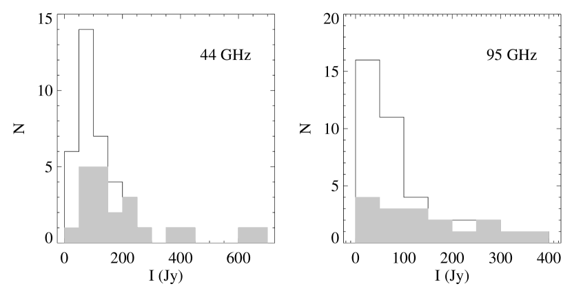
Figure 1: Number density distributions of the total intensity (Stokes I) of the observed (solid lines) and the polarization-detected sources (grey filled area) at 44 (left) and 95 GHz (right). 

Figure 2: Number density distributions of the polarization fractions at 44 (left) and 95 GHz (right). 

Figure 3: Polarization fraction $P_{L}$ vs. Stokes I at 44 (left) and 95 GHz (right). The filled circles are those detected above $3\sigma$ errors, while open circles show the upper limits of polarization non-detected sources. Errors of $1\sigma$ are presented. 

Figure 4 presents the spectral profiles of the total flux $(I)$, the polarized intensity $(PI)$, the polarization degree ($P_{L}$), and the polarization position angle measured counterclockwise from north ($\chi$) of the sources detected at both transitions. The profiles of the total flux and the polarized intensity tend to peak at similar velocities with some exceptions like G40.25-0.19 (Fig. 4$l$ at 44 GHz). Some sources, e.g., G18.34+1.78SW (Fig. 4$f$), have multiple velocity components with different polarization properties. Figure 8 and Figure 9 show the same parameters for the sources detected only at 44 or 95 GHz, respectively.

The measured polarization properties are summarized in Table 3. The presented values of $F_{\nu}$, $P_{L}$, $\chi$, and $v_{\rm LSR}$ are all determined in the channel with the peak polarized intensity. The amplitude or the phase of a vector does not have a Gaussian probability distribution unless the signal-to-noise ratio is very large. This can lead to systematic errors in the measured polarizations. According to Wardle & Kronberg (1974), the best estimates of the true polarization can be found using $R\sim{R_{M}}^{\prime}[1-(\sigma^{\prime}/{R_{M}}^{\prime})^{2}]^{1/2}$ for $R/\sigma^{\prime}>0.5$, where ${R_{M}}^{\prime}$ is the observed polarization and $\sigma^{\prime}$ is the observed random noise. Random noise does not produce a bias in $\chi$ but increases the error of $\chi$ by $\sigma_{\chi}\simeq\sigma^{\prime}/{R_{M}}^{\prime}$ radians. We corrected for these effects in the presented $P_{L}$ and $\chi$. The amount of correction in $P_{L}$ is insignificant in our cases, but $\sigma_{\chi}$ normally exceeds the measurement error. Errors presented are $1\sigma$.

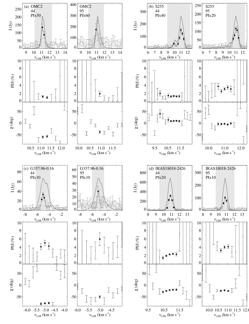
Figure 4: Polarization-detected masers at both transitions. The source name and line frequency are indicated in each panel. For each source, the polarized intensity $(PI)$ in grey line with errors (1$\sigma$) and the total flux intensity $(I)$ in black solid line (top), and the polarization fraction $P_{L}$ (middle) and angle $\chi$ (bottom) are presented. The multiplication factor of $PI$ is presented under the line frequency for each source. The points with $PI>3\sigma$ are indicated with filled circles. The grey-shaded area in the top panel indicates the velocity range for the middle and bottom panels.

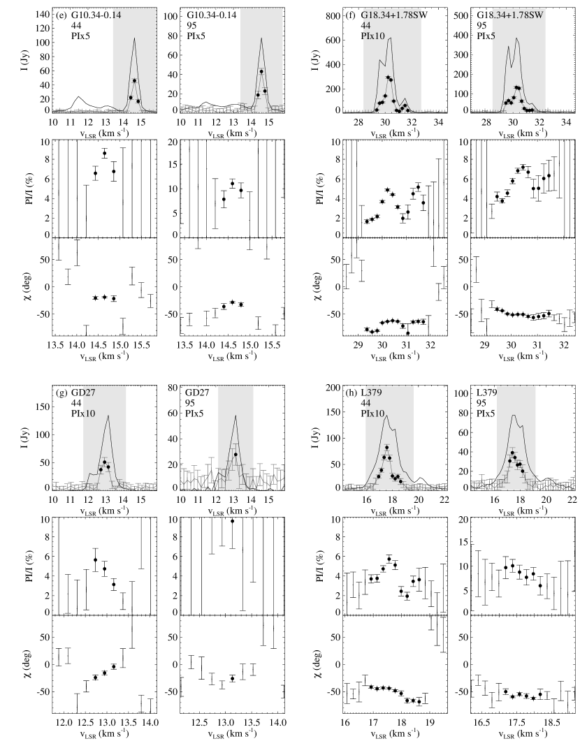
Figure 4: (continued)

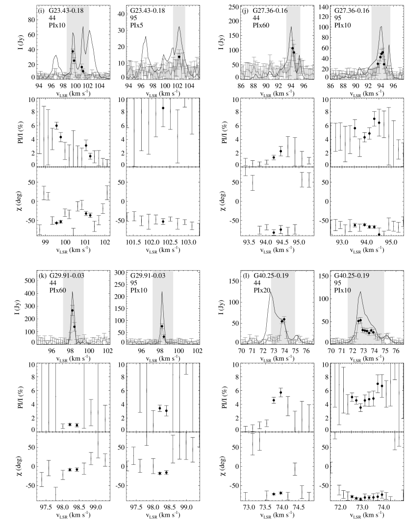
Figure 4: (continued)

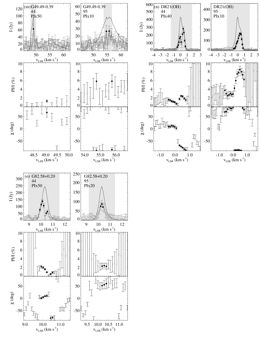
Figure 4: (continued)

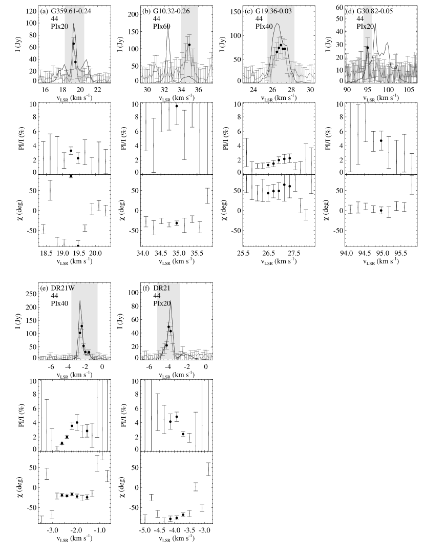
Figure 8: Polarization-detected sources only at 44 GHz.

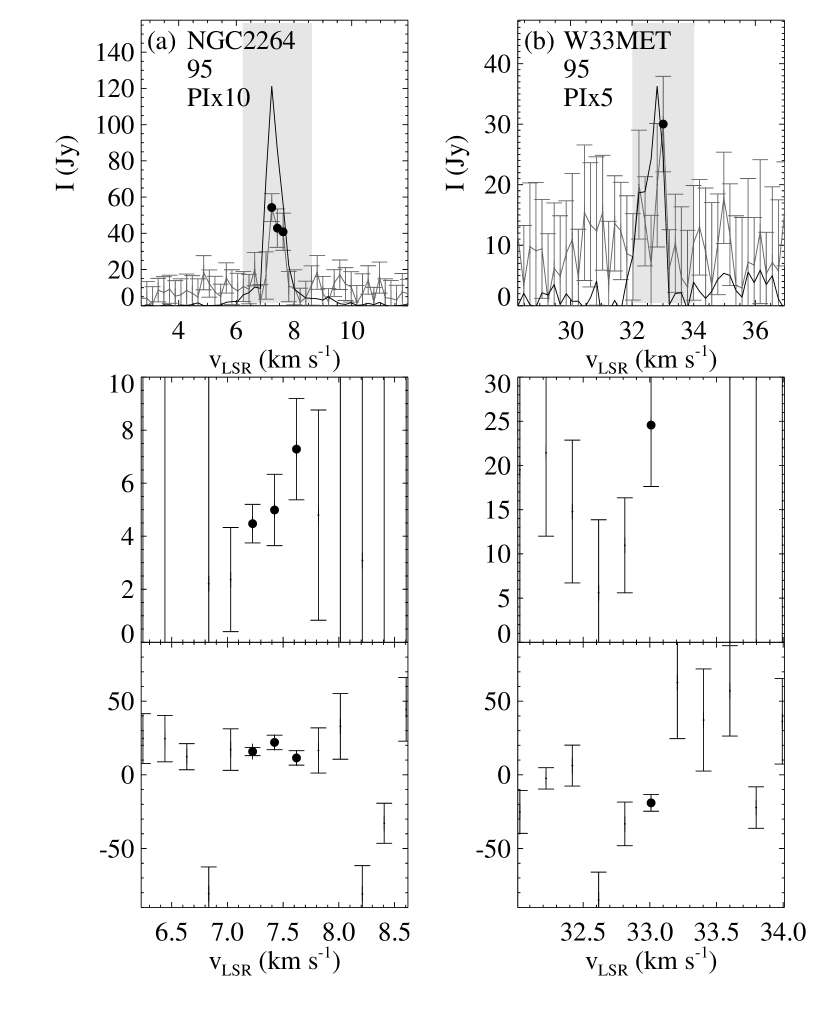
Figure 9: Polarization-detected sources only at 95 GHz.

Table 3: Linear Polarization Properties 

Source	Transition	$F\nu$	$P_{L}$	$\chi$	$v_{\rm LSR}$
Name	( GHz )	( Jy )	( % )	( ∘ )	( km s-1 )
OMC2	44	$205.6\pm 2.8$	$1.3\pm 0.4$	$120\pm 9$	$+11.1$
	95	$147.8\pm 5.1$	$2.0\tablenotemark{a}\pm 0.7$	$142\pm 8$	$+10.9$
S255N	44	$263.4\pm 0.8$	$1.4\pm 0.3$	$9\pm 5$	$+11.0$
	95	$188.1\pm 0.7$	$3.1\pm 0.3$	$176\pm 4$	$+11.0$
NGC2264	95	$121.3\pm 4.0$	$4.5\pm 0.9$	$15\pm 10$	$+7.2$
G357.96-0.16	44	$67.0\pm 0.4$	$5.0\pm 0.6$	$102\pm 8$	$-5.0$
	95	$47.7\pm 0.8$	$5.9\pm 1.5$	$129\pm 10$	$-5.0$
G359.61-0.24	44	$99.4\pm 1.4$	$3.3\pm 0.5$	$85\pm 9$	$+19.3$
IRAS18018-2426	44	$685.0\pm 5.5$	$2.3\pm 0.6$	$158\pm 3$	$+10.9$
	95	$255.3\pm 1.2$	$4.0\pm 0.6$	$157\pm 4$	$+10.8$
G10.34-0.14	44	$106.7\pm 0.7$	$8.6\pm 0.5$	$161\pm 3$	$+14.6$
	95	$78.0\pm 1.8$	$11.0\pm 1.0$	$151\pm 3$	$+14.6$
G10.32-0.26	44	$19.6\pm 0.4$	$9.5\pm 2.6$	$148\pm 18$	$+34.9$
W33MET	95	$24.4\pm 1.5$	$24.6\pm 6.9$	$160\pm 19$	$+33.0$
G18.34+1.78SW	44	$604.2\pm 5.7$	$4.9\pm 0.5$	$116\pm 1$	$+30.2$
	95	$387.3\pm 1.9$	$6.8\pm 0.5$	$129\pm 2$	$+30.3$
GGD27	44	$107.9\pm 1.0$	$4.7\pm 0.8$	$164\pm 8$	$+12.9$
	95	$58.3\pm 3.6$	$9.6\pm 2.8$	$153\pm 7$	$+13.1$
G19.36-0.03	44	$99.9\pm 0.7$	$2.0\pm 0.5$	$48\pm 21$	$+26.9$
L379	44	$143.8\pm 1.8$	$5.7\pm 0.5$	$136\pm 4$	$+17.6$
	95	$77.6\pm 3.1$	$10.1\pm 1.3$	$120\pm 5$	$+17.4$
G23.43-0.18	44	$62.9\pm 0.8$	$6.0\pm 0.5$	$123\pm 6$	$+99.6$
	95	$32.3\pm 1.1$	$8.5\pm 2.7$	$127\pm 8$	$+102.3$
G27.36-0.16	44	$129.4\pm 2.5$	$1.4\pm 0.4$	$98\pm 13$	$+94.2$
	95	$74.1\pm 0.8$	$7.0\pm 1.1$	$113\pm 5$	$+94.3$
G29.91-0.03	44	$414.9\pm 2.7$	$1.1\pm 0.5$	$171\pm 6$	$+98.2$
	95	$220.9\pm 4.0$	$3.4\pm 0.5$	$161\pm 4$	$+98.2$
G30.82-0.05	44	$29.1\pm 0.6$	$4.7\pm 1.3$	$0\pm 18$	$+95.0$
G40.25-0.19	44	$52.0\pm 0.6$	$5.7\pm 0.6$	$110\pm 8$	$+74.0$
	95	$116.0\pm 3.5$	$4.6\pm 0.5$	$96\pm 4$	$+72.7$
G49.49-0.39	44	$97.1\pm 2.0$	$1.3\pm 0.3$	$66\pm 19$	$+49.1$
	95	$46.0\pm 0.7$	$5.8\pm 1.5$	$94\pm 10$	$+55.7$
DR21W	44	$159.3\pm 1.7$	$2.0\pm 0.2$	$159\pm 4$	$-2.4$
DR21(OH)	44	$294.1\pm 2.9$	$2.1\pm 0.2$	$109\pm 3$	$+0.4$
	95	$201.7\pm 5.7$	$8.2\pm 0.8$	$92\pm 2$	$+0.4$
DR21	44	$51.0\pm 1.3$	$4.8\pm 0.7$	$103\pm 8$	$-3.9$
G82.58+0.20	44	$144.0\pm 1.3$	$1.8\pm 0.2$	$6\pm 5$	$+10.1$
	95	$168.6\pm 3.2$	$2.5\tablenotemark{a}\pm 0.5$	$55\pm 16$	$+10.3$

Note. — The presented values of $F_{\nu}$, $P_{L}$, $\chi$, and $v_{\rm LSR}$ are all determined in the channel with the peak polarized intensity.

The polarization properties of the 44 and the 95 GHz methanol masers are observed to be well correlated. In Figure 10, the polarization degrees of the two transitions appear to have a positive linear correlation, although the correlation is not very tight. Their linear Pearson correlation coefficient is $r=0.71$, where $r=0$ and $1$ indicate no correlation and a perfect positive linear correlation, respectively. The polarization fractions of the 95 GHz masers tend to be greater than those of the 44 GHz masers. This is consistent with the finding of Wiesemeyer et al. (2004), where the polarization fraction at higher frequency transition is higher than that at lower frequency whenever a source is detected at multiple maser transitions. Figure 10 compares the position angles of the 44 and the 95 GHz maser transitions as well. Their correlation coefficient is $r=0.92$, indicating that their position angels are generally well correlated.

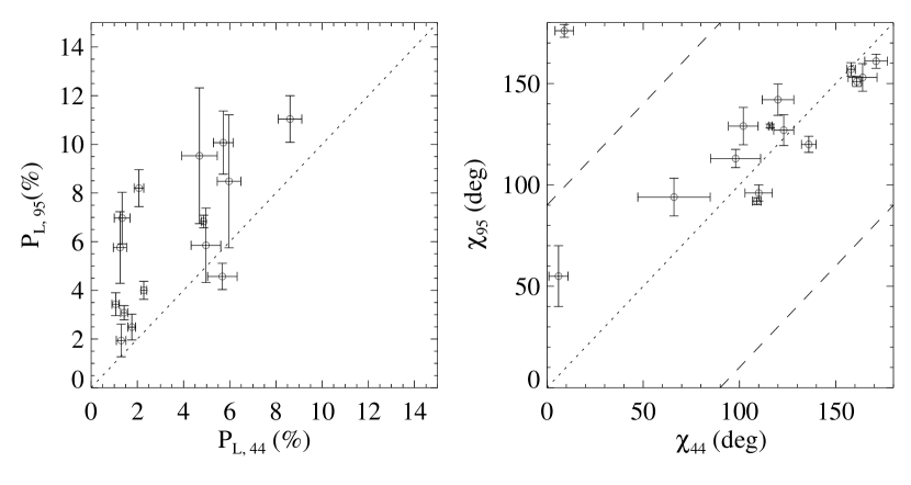
Figure 10: 44 GHz vs. 95 GHz masers in polarization fraction, $P_{L}$ (left) and angle, $\chi$ (right) for the sources detected in both transitions at the same velocities. Errors of $1\sigma$ are presented. The dotted lines show the cases when the polarization degree and angles of the two transitions are the same. The dashed lines in the right panel show the cases when the angels are $90^{\circ}$ different.  

4 Discussion

4.1 The Measured Polarization Properties

About 40% of the observed sources did not show any linear polarization in either of the two transitions. Because of the observational limitations such as sensitivity and a large single dish beam depolarizing multiple maser features with different orientations, we can not exclude the presence of linear polarization even for the non-detected sources.

The measured linear polarization fractions in this study are mostly less than 10%. The fractions could be lower limits, because there are several effects reducing the original degree of linear polarization. Linear polarization can be reduced by field line curvature along the propagation direction by destroying the phase coherence of polarization (Elitzur, 2002), or by internal Faraday rotation due to the presence of electrons in the magnetized medium along the maser amplification path (Fish & Reid, 2006). However, the effects of internal Faraday rotation is expected to be small (Surcis et al., 2011), so our results are not likely affected by the Faraday rotation. The fraction can also be reduced by depolarization because of combining multiple maser features with different polarization orientations within a large single dish beam.

None of the 5 sources detected at 84 GHz or 95 GHz by Wiesemeyer et al. (2004) were detected in our 95 GHz observations, although some targets have high fractional polarizations up to $\sim 9$%. This is mainly because of the sensitivity issue. Four (S231, W51Met2, W75S(3), and NGC7538) were weak sources with total fluxes below 20 Jy, and could not be detected in our 95 GHz observations with a typical rms of 1.2 Jy and the $3\sigma$ detection criterion. The other (DR21W) was bright (210 Jy) but was rejected from the detection list because it had a polarization fraction slightly lower than the upper limit (2%) of the artificial system polarization at 95 GHz.

We have not detected any source with linear polarization above 30% that Wiesemeyer et al. (2004) has reported at 132 GHz Class I and 157 GHz Class II maser transitions. The highest estimated linear polarization degrees were 40% and 37% at 132 and 157 GHz, respectively. Linear polarization above 33% is expected to be rare (Elitzur, 2002). It is possible only when the angle between the magnetic field and the ray path is $35^{\circ}<\theta<45^{\circ}$ for isotropic pumping. Nedoluha & Watson (1990) indicated that, for an angular momentum $J=1-0$ transition, the fractional polarization as high as 100% is observable when a Zeeman frequency is large, however, about 30% would be the highest for an angular momentum $J=2-1$ and higher transitions, unless significant anisotropic pumping is present. Wiesemeyer et al. (2004) found that a large fractional linear polarization $(P_{L}>33\%)$ is not rare ( 2 out of 10 for Class I and 1 out of 3 for Class II), giving an impression that anisotropic pumping or loss may be commonly achievable due to an unequal population of the magnetic substates of the maser levels (Nedoluha & Watson, 1990). In the present study, none of 23 polarization detected sources show such high linear polarization. We also observed 2 sources (M8E and L379) that showed highest fractional polarization $>30$% at 132 GHz in Wiesemeyer et al. (2004). The two have fractional polarizations of 4% – 10% at 95 GHz. Since transitions at higher frequencies tend to have higher fraction of polarization, we cannot directly compare our results with those of Wiesemeyer et al. (2004). However, our observational results, none with such high fractional polarization out of 23 polarization detected sources, still suggest that the anisotropic pumping or loss mechanism may not be common for 44 and 95 GHz maser transitions.

4.2 Comparison of Polarization Properties at 44 and 95 GHz

We have found that the polarization fractions and angles of the 44 and 95 GHz masers are generally well correlated as shown in Figure 10. Their fractions of linear polarization tend to have a linear correlation and their polarization angles are aligned well. It has been suggested that the two transitions trace similar regions (e.g., Val’tts et al., 2000; Kang et al., 2015). The similar polarization properties of the two lines also confirm that the masers at these two transition lines are indeed experiencing magnetic fields of similar regions.

Our observations show that the degree of linear polarization at 95 GHz is greater than that at 44 GHz for all 15 sources detected at both frequencies with one exception (G40.25$-$0.19). The reduced fractional polarization at the lower frequency transition compared to higher frequency transitions seems to be general trend in maser polarization observations. For example, McIntosh & Predmore (1993) and Wiesemeyer et al. (2004) reported the same trend for silicon monoxide and methanol masers, respectively. Several possibilities may be suggested to explain these observations.

The Faraday rotation is suggested as an explanation of depolarization at longer wavelengths (Elitzur, 2002). The effects of Faraday rotation on the linear polarization of the masers are well described by Fish & Reid (2006) and Surcis et al. (2011). According to their explanation, internal Faraday rotation due to the free electrons in the path of maser amplification can decrease the linear polarization fraction of the radiation, sometimes completely circularizing it if the Faraday rotation is strong enough (Goldreich et al., 1973). However, Surcis et al. (2011) show that the depolarization due to the internal Faraday rotation for the 6.7 GHz methanol maser is negligible in case of C-shock, and it is not likely significant in case of J-shock either. The rotation measure changes due to the external Faraday rotation is negligibly small to produce depolarization. When $RM=1100~{}{\rm rad~{}m^{-2}}$, the maximum value measured toward pulsars in Han et al. (2006), is adopted, the angle due to the Faraday rotation is only $3^{\circ}$ at 44 GHz, which in general smaller or comparable to the angle measurement error. Thus, the Faraday rotation can not explain the lower polarization fraction at 44 GHz.

Another possibility is the lower $J$ transition data averaging over a larger volume of medium due to the larger beam than the other transitions (McIntosh & Predmore, 1993). Variation of physical conditions in a larger volume may reduce the fractional polarization. However, the similarities in total flux and polarization properties in our observations suggest that both transitions are likely covering similar maser components. In addition, according to the previous VLA observations (Kogan & Slysh, 1998; Kurtz et al., 2004) of methanol masers, a case of the 44 GHz masers being distributed over area wider than the KVN beam, $30^{{}^{\prime\prime}}$ at 95 GHz, is rare. Thus, different volume does not seem to be the main cause of the difference of fractional polarization.

The fractional linear polarization of the 44 and 95 GHz transitions could be intrinsically different. Pérez-Sánchez & Vlemmings (2013) calculated the fractional linear polarization as a function of the emerging brightness temperature for some rotational transitions of SiO, H₂O and HCN masers. In their calculation, the higher $J$ transitions have somewhat lower polarization percentages, which is mainly due to the averaging over more magnetic substates. However, this assumes similar levels of stimulated emission rate, $R$. As also shown in Nedoluha & Watson (1990), the linear polarization fraction is a function of the degree of maser saturation $R/\Gamma$, a ratio of stimulated emission rate to decay rate, and the angle $\theta$ between the line of sight (LOS) and the magnetic field orientation. One of their main finding is that the polarization characteristics for high $J$ transitions are similar in quality and quantity, suggesting the behaviors of the $7_{0}-6_{1}A+$ and $8_{0}-7_{1}A+$ transitions would be similar as long as they have similar saturation level and $\theta$. The angle $\theta$ is likely to be similar for both transitions. Although not much is known about the decay rate of the masers (Vlemmings et al., 2010), in our case, $R$ is also similar for both maser transitions. The stimulated emission rate $R$ is given by $R\sim\frac{AkT_{b}\Delta\Omega}{4\pi h\nu}$, where A is the Einstein coefficient of the involved transition, $k$ and $h$ are the Boltzmann and Planck constant, $\nu$ is the maser frequency, $T_{b}$ is the brightness temperature, and $\Delta\Omega$ is the relation between the real angular size of the masing cloud and the observed angular size (Pérez-Sánchez & Vlemmings, 2013). The Einstein coefficients are $A_{\rm 44~{}GHz}\sim 2.74\times 10^{-7}$ s^-1, and $A_{\rm 95~{}GHz}\sim 2.87\times 10^{-6}$ s^-1 (Lankhaar et al., 2016, in prep.). The brightness temperature $T_{b}$ can be estimated using $T_{b}=S_{\nu}\Sigma^{-2}\zeta_{\nu}$, where $S_{\nu}$ is the observed flux density, $\Sigma$ is the maser angular size, and $\zeta_{\nu}$ is a constant factor that includes a proportionality factor obtained for a Gaussian shape. This factor $\zeta_{\nu}\propto\nu^{-2}$, and is $\sim 3.16\times 10^{8}$ at 44 GHz and $\sim 6.77\times 10^{7}$ at 95 GHz respectively (Pérez-Sánchez & Vlemmings, 2013). Thus, $T_{b}$ is roughly five times larger at 44 GHz than at 95 GHz when assuming the same physical size and flux. When additionally the same beaming angle is assumed, the stimulated emission rate $R_{\rm 44~{}GHz}\approx 0.96~{}R_{\rm 95~{}GHz}$. As the flux of the 95 GHz masers is found to be $\sim 50\%-80\%$ of that of the 44 GHz masers, $R_{\rm 44~{}GHz}$ for the individual masers is unlikely to be more than $\sim 2\times R_{\rm 95~{}GHz}$. Saturation effects are thus unlikely to contribute to the observed differences unless the physical sizes of the masers and/or the beaming angles of the two transitions are very different. Related to this, the dependence of the linear polarization on the ratio between the Zeeman splitting rate and the stimulated emission rate, $g\Omega/R$, can still contribute to the observed differences between the two maser transitions (Nedoluha & Watson, 1990), provided $g\Omega$ is sufficiently different between the two transitions. Full understanding on the intrinsic cause of higher polarization fraction in higher frequency transition line seems to need supports from the theoretical studies in the future.

4.3 Association with Outflows or Galactic Scale Magnetic Fields

Class I methanol masers are collisionally excited and thought to occur in the areas where the methanol molecular abundance is enhanced by the outflow shock heating of grain mantles (Menten, 1991). If they arise in the regions compressed by outflow shock, then the observed polarization angles could be associated with the orientations of outflows. We have searched for the references related to the outflows of the 23 polarization detected sources using the SIMBAD website (Wenger et al., 2000). Many sources have references indicating existence of outflows, such as H₂ maps, extended green objects, or outflow tracing molecular line observations, but directions of outflows are not obvious in many cases. Among them, we have found 7 sources, i.e., OMC2, S255N, NGC2264, G49.49$-$0.39 (W51 e2), DR21W, DR21, and DR21(OH), where the direction of maser-associated outflow is rather simple. IRAS18018-2426, GGD27, L379, and G30.82-0.05 (W42 main) have been mapped in CO transition lines as well, but the connection between the maser and outflow is not obvious either due to the outflow direction being in the line-of-sight or due to the complicated multiple outflows morphology (Zhang et al., 2005; Fernández-López et al., 2013; Kelly & MacDonald, 1996; Sridharan et al., 2014).

We have compared the polarization angles at 44 GHz for 6 sources and at 95 GHz for NGC2264, which are not detected at 44 GHz, with the orientations of outflows available in the literatures. The position angles (PA) of their outflows, their references, and the angles between the polarization angle and the outflow are summarized in Table  4. Regarding the errors of $|\chi-PA_{\rm out}|$, we took the measurement errors of the polarization angles, but the errors would be larger considering that the errors of outflows are normally larger. For example, the conventional error of outflow is considered to be $15^{\circ}$ in Surcis et al. (2013). There are some sources with their polarization angles being almost perpendicular to the outflow direction, e.g., OMC2 and DR21W. However, in general, the association between outflows and polarization angles is not apparent.

Although the sample size is small, we tried the Kolmogorov-Smirnov (K-S) statistics to see whether the angle differences are similar to or different from the projected angles of aligned, perpendicular, or randomly aligned samples, by comparing the observed angle difference to the results from the Monte Carlo simulations as discussed in Hull et al. (2014). The simulation that randomly selects pairs of vectors in three dimensions gives the same distribution when it is projected on the plane of the sky. However, the projection effects increase the scatter of 2-d projected angles in other cases. For the aligned case, we select pairs of vectors that are aligned within $20^{\circ}$ of one another among the random pairs in three dimensions and calculate their angles projected onto the plane of the sky. For the perpendicular case, we select pairs of vectors separated by $70^{\circ}-90^{\circ}$, and projected them. The projection effects are more important in the perpendicular case then those in the aligned case. The cumulative distribution functions (CDF) of the 2-d projected angles from simulations are compared with the CDF of the observed angle difference between the outflow direction and the polarization angle in the left panel of Figure 11.

Table 4: Outflow Orientations and Polarization Angles

Source Name	$\chi$	$PA_{\rm out}$	$|\chi-PA_{\rm out}|$	Reference
OMC2	$120^{\circ}$	$30^{\circ}$	$90^{\circ}\pm 9^{\circ}$	Williams et al. (2003)
S255N	$9^{\circ}$	$51^{\circ}$	$42^{\circ}\pm 5^{\circ}$	Wang et al. (2011)
NGC2264	$15^{\circ}$	$175^{\circ}$	$20^{\circ}\pm 10^{\circ}$	Schreyer et al. (2003)
G49.49$-$0.39 (W51 e2)	$66^{\circ}$	$137^{\circ}$	$71^{\circ}\pm 19^{\circ}$	Shi et al. (2010)
DR21W	$159^{\circ}$	$70^{\circ}$	$89^{\circ}\pm 4^{\circ}$	Garden et al. (1991)
DR21(OH)	$109^{\circ}/36^{\circ}$	$113^{\circ}$	$4^{\circ}\pm 3^{\circ}/77^{\circ}\pm 3^{\circ}$	Zhang et al. (2014)
DR21	$103^{\circ}$	$150^{\circ}$	$47^{\circ}\pm 8^{\circ}$	Garden et al. (1991)

Note. — $\chi$ at 44 GHz is used for comparison except NGC2264, which is polarization detected only at 95 GHz. Position Angels of outflows (PA_out) are estimated counterclockwise from the north, same as the way that the polarization angles of 44 GHz masers are measured. The reference for the outflow orientation is noted in the Reference column. The error of the PA difference in column 4 is adopted from the 44 GHz maser polarization angle measurement error. DR21(OH) has two perpendicular polarization angles, resulting in two perpendicular $|\chi-PA_{\rm out}|$ values.

Figure 11: Thick solid lines show the cumulative distribution functions (CDF) of the angles between the polarization angles and the orientations of outflows (left) and those of the Galactic pole (right). The dotted line and dashed and long-dashed curves are the CDFs of projected angles from Monte Carlo simulations where two vectors are randomly distributed, perpendicular, and well-aligned to each other, respectively. 

The probabilities of the observed $|\chi-PA_{\rm out}|$ and the simulated projected angles being different or similar derived from the K-S tests are given in Table 5. The K-S tests rule out the scenario where the outflows and polarization angles are tightly aligned $(P<0.01)$. The probability of them being perpendicular $(P=0.7)$ appears to be higher than that of them being random $(P=0.4)$. Magnetic fields could be either parallel or perpendicular to the polarization angle depending on the angle between the magnetic field and the ray path, $\theta$. If we simply assume that methanol masers are strongly saturated $(R/\Gamma>10^{2})$ because they are strong, then the polarization angle is perpendicular to the magnetic field regardless of $\theta$ (Nedoluha & Watson, 1990). If we perform the K-S tests for $|B-PA_{\rm out}|$ taking into account above assumption, the K-S tests returns $P=0.5$ for random, and $P<0.1$ for aligned and perpendicular cases of simulations. Considering the ambiguity of magnetic field direction derived from the polarization angle, limited number of samples, and the difficulty of distinguishing the projected angle distribution from the random and $70^{\circ}-90^{\circ}$ simulations, we cannot conclude whether magnetic fields/polarization angles are randomly aligned or mis-aligned with outflows, however, we can rule out the scenario of them being tightly aligned at least.

Table 5: Probability of the K-S Test 

	$|\chi-PA_{\rm out}|$	$|\chi-PA_{\rm GPole}|$
random	P = 0.4	P = 0.3
$0^{\circ}-20^{\circ}$	$<0.01$	$<0.01$
$70^{\circ}-90^{\circ}$	0.7	$<0.01$

Note. — Probability is a value between 0 and 1 giving the significance level of the K-S statistics. Small values of probability indicate that the CDFs of the two data sets are significantly different from one another.

Maser emitting regions are very small in size so that the magnetic fields traced by masers are not expected to be associated with the magnetic field in Galactic or molecular cloud scales. However, there have been some studies showing that the field orientations measured from the Zeeman effect of OH masers in the star forming regions have positive correlation with the Galactic scale magnetic field measured from Faraday rotations (e.g., Han & Zhang, 2007; Fish & Reid, 2006; Noutsos, 2012). Since Class I methanol masers occur in a medium of similar or slightly less density, and at larger distance from the central stars, than the OH masers, we have investigated the possibility of association between the linear polarization of the 44 GHz methanol masers and the orientation of the Galactic pole, which could be related to the large scale magnetic field.

We apply the same analysis that is done for the outflows. As seen in the right panel of Figure 11, the CDF of the angle between the polarization angle and the direction of Galactic pole, $|\chi-PA_{\rm GPole}|$, is similar neither with the CDF of $0^{\circ}-20^{\circ}$ simulation nor with that of $70^{\circ}-90^{\circ}$ simulation. The K-S tests also retune $P<0.01$ for these two cases (Table 5), ruling out the scenario of the polarization angles having preference on the directions of Galactic plane or pole.

5 Discussion on Sources with Peculiar Polarization Properties

We discuss some interesting targets with unique polarization characteristics in detail.

5.1 G10.32$-$0.26

The linear polarization of G10.32$-$0.26 is detected only at 44 GHz (see Fig. 8$b$). It is peculiar because the linear polarization is not detected in the brightest peak of the total flux profile at $v_{\rm LSR}$ $\sim 32.5$ km s^-1 (A component in Fig. 12$a$) with an upper limit of 0.9%, but its secondary peak at $v_{\rm LSR}$ $\sim 35$ km s^-1 (B component in Fig. 12$a$) shows polarization. We confirmed this trend by observing them in two or more epochs. As mentioned in § 2.1, our observations were targeted for the brightest features in the total intensity. If the weaker feature is largely displaced from the brightest one, for example, by 30″, that could produce artificial polarization of up to 2%. The displacement of the 35 km s^-1 component from the brightest peak is less than 1″, according to the VLBI observation using the KVN and VERA combined array (KaVA) (Kim et al. in prep.) and its observed degree of polarization is 4 – 9%, which are well above the 2%. Thus, these detections are very likely real.

Figure 12: Multiple maser components of (a) G10.32$-$0.26, (b) G18.34+1.78SW, and (c) G40.25$-$0.19 described in Section 5. The solid line indicates the 44 GHz total flux profile of each source. Individual components described in the text of Section 5 are marked as A, B, or C and indicated with arrows. The filled circles indicate the points with $PI_{44GHz}>3\sigma$ after 10 times of multiplication. The open circles are same but at 95 GHz.

5.2 G18.34+1.78SW

G18.34+1.78SW is one of the brightest methanol masers known in the Galaxy first detected in the KVN single dish maser surveys (Kim et al. in prep.). It is associated with millimeter core MM2 in a massive star forming region IRAS 18151-1208 (Marseille et al., 2008). It is imaged by the KaVA at an angular resolution of $\sim$2 milli-arcsecond (Matsumoto et al., 2014).

The single-dish total intensity spectra of G18.34+1.78SW show 3 maser features with peak velocities of $+30.3$ (A) $+29.6$ (B), and +31.4 km s^-1 (C in Fig. 12$b$) in both transitions, all of which show linearly polarized emission in both transitions (see also Fig. 4$f$). The velocities of these 3 components are well agreed with the findings of Matsumoto et al. (2014), although much of the total flux was missed in the VLBI image. The polarization properties of these 3 components are summarized in Table 6. We used a function with 3 Gaussian components to fit the 0.1 km s^-1 resolution spectra. The line widths measured in the polarization profile range between 0.4 and 0.6 km s^-1 , while it is 0.2 km s^-1 wider when measured in the total flux profile.

This object has $P_{L}=2.0-6.8$% in two transitions, and all 3 components show slightly higher polarization at 95 GHz, which is generally observed for other sources. The polarization angles of the brightest peak are similar at 44 and 95 GHz, i.e., $12^{\circ}$ different, but the difference is beyond the measure error. The angle difference ranges up to $43^{\circ}$ in the second brightest peak. The fact that the polarization angle differences are not consistent for the 3 maser features in a nearly same position, at most 100 mas apart (Matsumoto et al., 2014), indicates that neither rotation measure nor the beam size can explain the difference in the polarization properties of the 44/95 GHz transitions. It may be a combination of magnetic field morphology and the saturation level difference between the two transition lines as discussed in section 4.2. High resolution line polarimetry using the VLA or ALMA will help us to understand the underlying physics.

Table 6: Polarization Properties of G18.34+1.78SW

$v_{\rm LSR}$	Transition	$I$	$P_{L}$	$\chi$	$\Delta v_{\rm FWHM}$
( km s-1 )	( GHz )	( Jy )	( % )	( ∘ )	( km s-1 )
+30.3	44	678.	$4.8\pm 0.1$	$118\pm 1$	0.5
	95	411.	$6.8\pm 0.2$	$130\pm 1$	0.6
+29.6	44	471.	$2.0\pm 0.1$	$96\pm 1$	0.4
	95	346.	$3.6\pm 0.2$	$139\pm 1$	0.5
+31.4	44	124.	$5.4\pm 0.4$	$117\pm 2$	0.4
	95	50.	$6.2\pm 2.4$	$132\pm 8$	0.5

Note. — Spectra with 0.1 km s^-1 resolution were used for Gaussian fit. The $v_{\rm FWHM}$ presented is the fitting result of polarized intensity profile, which is 0.2 km s^-1 smaller in maximum than that of total intensity profile.

5.3 G40.25$-$0.19

The single dish total intensity profiles of G40.25$-$0.19 show multiple maser components at $v_{\rm LSR}$ $=+72-+75.5$ km s^-1 at both transitions (see Fig. 4$l$ and Fig. 12$c$). This target is interesting because it shows linear polarization degrees of 4.5% – 7% at 95 GHz in all maser components at $v_{\rm LSR}$ $=+72-+75.5$ km s^-1 , but only a secondary bright feature at $v_{\rm LSR}$ $\sim 73.8$ km s^-1 (B in Fig. 12$c$) is detected at 44 GHz. The upper limit of the brightest peak at $v_{\rm LSR}$ $\sim 72.5$ km s^-1 (A) is 0.8%. The difference in polarizaton properties could also be related to maser saturation level for this source.

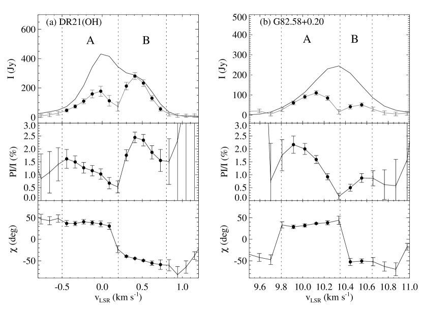
Figure 13: The polarization profiles of (a) DR21(OH) and (b) G82.58+0.20 at 44 GHz that show the polarization angle flips as described in Section 5. The explanations for the figures are same as Fig. 4, but zoomed in velocity ranges. The polarized intensities are 40 times multiplied. Two components showing the $90^{\circ}$ angle flips are marked as A and B after divided by dotted lines.

5.4 DR21(OH)

The 44 GHz masers of DR21(OH) have been imaged with the VLA (Kogan & Slysh, 1998; Kurtz et al., 2004). The VLA results show that there are two groups of masers, one at $v_{\rm LSR}$ $\sim 0$ km s^-1 and the other at $v_{\rm LSR}$ $\sim-4$ km s^-1 , about $20\arcsec$ apart from each other. These two groups of masers are located at the end of approaching and receding outflow in the DR21(OH) region (Zhang et al., 2014), supporting the theory of Class I methanol masers being stimulated by outflows. Our observation was pointed to the brightest peak at $v_{\rm LSR}$ $\sim 0$ km s^-1 that contains $\sim 80$% of the total flux and is located at the end of an receding outflow lobe. This feature has an elongated, arc-shape morphology in the VLA map.

The linear polarization of DR21(OH) shows features indicating depolarization and a sudden flip of polarization angle in the 44 GHz transition line. The total intensity and the polarized emission of DR21(OH) at 44 GHz show two maser components, one at $v_{\rm LSR}$ = $-0.5-+0.2$ km s^-1 and the other at $v_{\rm LSR}$ = +0.2 – +0.8 km s^-1 , which are indicated as A and B regions in the panel (a) of Figure 13. Their polarization fractions are similar to be $\sim 2$%, while their polarization angles are different by $\sim 90^{\circ}$. At the velocity where the two components overlapped, the fraction of linear polarization drops to minimum.

Taking into account the previous observations, elongated masers aligned along a curved receding shock front with the magnetic field compressed along the shock can explain the observed profiles. Such flip of polarization angle is expected around $\theta=55^{\circ}$ in maser theories(e.g., Goldreich et al., 1973), and has been observed previously in SiO masers by Kemball & Diamond (1997) and in H₂O by Vlemmings & Diamond (2006). In these observations, the angle flip appeared in a single maser feature, which was interpreted as an evidence of curved magnetic field with $\theta$ being close to the van Vleck angle, i.e., $\theta=55^{\circ}$. In our case, the flip happens in two different maser features separated in velocities in a single dish spectrum, but the underlying physics could be the same. If the two maser features are located in a curved magnetic field aligned along the shock front receding from us, each of their $\theta$ being $\theta<55^{\circ}$ and $\theta>55^{\circ}$, then, they would produce a 90^∘ angle flip as well as a LOS velocity shift that are observed. One implication of this explanation is that the 44 GHz masers of DR21(OH) is unsaturated or only moderately saturated according to the simulation of Nedoluha & Watson (1990). In the upper panels of Figure 3 in their paper, the polarization angle ($\phi$ in their paper) flips by the change of $\theta$ only when $\log R/\Gamma\lesssim 1$. When the maser is highly saturated, e.g., when $logR/\Gamma=3$, the polarization angle is not seriously affected by $\theta$ but rather constant.

The polarization angle can also be different as large as 90^∘ when the saturation levels of the two maser components are different. As seen in the Figure 3 of above paper, for example, if the saturation levels of the two components are $\log R/\Gamma$ = 1 and 3, respectively, the two components would show 90^∘ of polarization angle difference even for the same field orientation with $\theta=15^{\circ}$. How much the saturation levels of the same 44 GHz transition line can be different is another issue. Assuming the not-well-known factor $\Gamma$ being similar, $R$ would be determined by the physical size and the flux of maser components. The difference of the observed fluxes are less than factor of two different, while their physical sizes cannot be determined with current observations.

The angle flip is not observed in the 95 GHz transition line profile (see Fig 4$n$). While the polarization angle of the $-0.5-+0.1$ km s^-1 component at 95 GHz is almost perpendicular to that of the 44 GHz maser, the angle of the $+0.3-+0.7$ km s^-1 component is similar to that of the 44 GHz maser. If the angle flip in the 44 GHz maser is due to the van Vleck angle crossing, the polarization angles of the 95 GHz maser being relatively constant may imply that the 95 GHz transition is more highly saturated than the 44 GHz transition, in which condition, the position angle is always perpendicular to the magnetic field regardless of $\theta$, as Nedoluha & Watson (1990) demonstrated. The saturation levels of maser are difficult to be measured. Future high resolution observations and the theoretical study dedicated to the methanol maser lines would be able to reveal the morphology, field orientation, and kinematics of the DR21(OH) region as well as the involved maser physics.

5.5 G82.58+0.20

The polarization profiles of G82.58+0.20 present polarization intensity and angle variation similar to those of DR21(OH) at both transition lines. It shows polarization angle flip and the reduced polarization fraction at velocities where the two velocity components overlapped in the 44 GHz transition line, as indicated as A and B regions in the panel (b) of Figure 13. This may imply the existence of elongated masers associated with curved magnetic field orientation in a compressed medium. This target would be a good candidate for the high resolution polarimetry observations.

6 Summary

We performed the first comprehensive study of the linear polarization of a large sample of 39 bright Class I methanol maser sources in the 44 and 95 GHz transitions simultaneously. The main findings of this study are summarized as follows.

1. We detected 23 sources (59%) in at least one transition and 15 sources (38%) in both transition. Their error-weighted mean degrees of polarizations are $2.7\pm 0.3$% and $4.8\pm 0.1$% at 44 and 95 GHz, respectively. The linear polarization of the 44 GHz methanol maser transition was first detected in this study.

2. We compared the polarization properties of the 44 and 95 GHz transition lines. We found that their polarization fractions are linearly correlated, but the emission from the 95 GHz tends to be more linearly polarized than that from the 44 GHz transition line. We suggest that this is not likely due to the external reason, such as Faraday rotation or different beam size effect. The remaining possibility is the intrinsic differences of the physical parameters involved in the maser process, such as the decay rate, Zeeman rate, maser size, and beaming angle.

3. The polarization angles of the 44 and 95 GHz transition lines are well correlated in general, implying that both transitions are experiencing similar magnetic environment.

4. We did not observe any source with a fractional polarization $>30$%. Such high fractions were found by Wiesemeyer et al. (2004) and require anisotropic pumping/loss conditions. Our observations show that such conditions may be not as common in the star forming regions as Wiesemeyer et al. (2004) suggested.

5. We found that the polarization angles tend to be aligned perpendicular to the outflows for the 7 maser sources with known outflow orientations. This requires more samples to be generalized. We also found that the maser polarization angles are not particularly correlated with the Galactic geometry.

6. We discussed some targets with peculiar polarization properties. Among them, DR21(OH) and G82.58+0.20 appear to be interesting targets because they show the $90^{\circ}$ polarization angle flip in the 44 GHz polarization profiles, while it is not visible in their 95 GHz polarization profiles. The high angular resolution polarimetry observations in both frequencies and the theoretical studies will reveal whether these polarization properties are due to the van Vleck angle crossing or change of maser saturation level, providing more information on the not-well-known methanol maser polarization physics.

References

- Aumont et al. (2010) Aumont, J., Conversi, L., Thum, C., et al. 2010, A&A, 514, A70
- Chapman et al. (2013) Chapman, N. L., Davidson, J. A., Goldsmith, P. F., et al. 2013, ApJ, 770, 151
- Crutcher (2012) Crutcher, R. M. 2012, ARA&A, 50, 29
- Elitzur (2002) Elitzur, M. 2002, in Astrophysical Spectropolarimetry, ed. J. Trujillo-Bueno, F. Moreno-Insertis, & F. Sánchez, 225–264
- Fernández-López et al. (2013) Fernández-López, M., Girart, J. M., Curiel, S., et al. 2013, ApJ, 778, 72
- Fish & Reid (2006) Fish, V. L., & Reid, M. J. 2006, ApJS, 164, 99
- Garden et al. (1991) Garden, R. P., Hayashi, M., Hasegawa, T., Gatley, I., & Kaifu, N. 1991, ApJ, 374, 540
- Goldreich et al. (1973) Goldreich, P., Keeley, D. A., & Kwan, J. Y. 1973, ApJ, 179, 111
- Gómez-Ruiz et al. (2016) Gómez-Ruiz, A. I., Kurtz, S. E., Araya, E. D., Hofner, P., & Loinard, L. 2016, ArXiv e-prints
- Han et al. (2006) Han, J. L., Manchester, R. N., Lyne, A. G., Qiao, G. J., & van Straten, W. 2006, ApJ, 642, 868
- Han & Zhang (2007) Han, J. L., & Zhang, J. S. 2007, A&A, 464, 609
- Hull et al. (2013) Hull, C. L. H., Plambeck, R. L., Bolatto, A. D., et al. 2013, ApJ, 768, 159
- Hull et al. (2014) Hull, C. L. H., Plambeck, R. L., Kwon, W., et al. 2014, ApJS, 213, 13
- Kang et al. (2015) Kang, H., Kim, K.-T., Byun, D.-Y., Lee, S., & Park, Y.-S. 2015, ApJS, 221, 6
- Kang et al. (2015) Kang, S., Lee, S.-S., & Byun, D.-Y. 2015, JKAS, 48, 257
- Kelly & MacDonald (1996) Kelly, M. L., & MacDonald, G. H. 1996, MNRAS, 282, 401
- Kemball & Diamond (1997) Kemball, A. J., & Diamond, P. J. 1997, ApJ, 481, L111
- Kim et al. (2012) Kim, K.-T., Byun, D.-Y., Bae, J.-H., et al. 2012, in IAU Symposium, Vol. 287, IAU Symposium, ed. R. S. Booth, W. H. T. Vlemmings, & E. M. L. Humphreys, 488–491
- Kim et al. (2011) Kim, K.-T., Byun, D.-Y., Je, D.-H., et al. 2011, Journal of Korean Astronomical Society, 44, 81
- Koch et al. (2010) Koch, P. M., Tang, Y.-W., & Ho, P. T. P. 2010, ApJ, 721, 815
- Kogan & Slysh (1998) Kogan, L., & Slysh, V. 1998, ApJ, 497, 800
- Kurtz et al. (2004) Kurtz, S., Hofner, P., & Álvarez, C. V. 2004, ApJS, 155, 149
- Lee et al. (2011) Lee, S.-S., Byun, D.-Y., Oh, C. S., et al. 2011, PASP, 123, 1398
- Mangum (2000) Mangum, J. G. 2000, User’s Manusal for the NRAO 12 Meter Millimeter-Wave Telescope, NRAO, 129
- Marseille et al. (2008) Marseille, M., Bontemps, S., Herpin, F., van der Tak, F. F. S., & Purcell, C. R. 2008, A&A, 488, 579
- Matsumoto et al. (2014) Matsumoto, N., Hirota, T., Sugiyama, K., et al. 2014, ArXiv e-prints
- McIntosh & Predmore (1993) McIntosh, G. C., & Predmore, C. R. 1993, ApJ, 404, L71
- Menten (1991) Menten, K. 1991, in Astronomical Society of the Pacific Conference Series, Vol. 16, Atoms, Ions and Molecules: New Results in Spectral Line Astrophysics, ed. A. D. Haschick & P. T. P. Ho, 119
- Nedoluha & Watson (1990) Nedoluha, G. E., & Watson, W. D. 1990, ApJ, 354, 660
- Noutsos (2012) Noutsos, A. 2012, Space Sci. Rev., 166, 307
- Oh et al. (2011) Oh, S.-J., Roh, D.-G., Wajima, K., et al. 2011, PASJ, 63, 1229
- Pérez-Sánchez & Vlemmings (2013) Pérez-Sánchez, A. F., & Vlemmings, W. H. T. 2013, A&A, 551, A15
- Plambeck & Menten (1990) Plambeck, R. L., & Menten, K. M. 1990, ApJ, 364, 555
- Sault et al. (1996) Sault, R. J., Hamaker, J. P., & Bregman, J. D., ApJS, 117, 149
- Sarma & Momjian (2011) Sarma, A. P., & Momjian, E. 2011, ApJ, 730, L5
- Schreyer et al. (2003) Schreyer, K., Stecklum, B., Linz, H., & Henning, T. 2003, ApJ, 599, 335
- Shi et al. (2010) Shi, H., Zhao, J.-H., & Han, J. L. 2010, ApJ, 718, L181
- Sridharan et al. (2014) Sridharan, T. K., Rao, R., Qiu, K., et al. 2014, ApJ, 783, L31
- Stephens et al. (2014) Stephens, I. W., Looney, L. W., Kwon, W., et al. 2014, Nature, 514, 597
- Surcis et al. (2011) Surcis, G., Vlemmings, W. H. T., Curiel, S., et al. 2011, A&A, 527, A48
- Surcis et al. (2012) Surcis, G., Vlemmings, W. H. T., van Langevelde, H. J., & Hutawarakorn Kramer, B. 2012, A&A, 541, A47
- Surcis et al. (2013) Surcis, G., Vlemmings, W. H. T., van Langevelde, H. J., Hutawarakorn Kramer, B., & Quiroga-Nuñez, L. H. 2013, A&A, 556, A73
- Tang et al. (2013) Tang, Y.-W., Ho, P. T. P., Koch, P. M., Guilloteau, S., & Dutrey, A. 2013, ApJ, 763, 135
- Val’tts et al. (2000) Val’tts, I. E., Ellingsen, S. P., Slysh, V. I., et al. 2000, MNRAS, 317, 315
- Vlemmings (2012) Vlemmings, W. H. T. 2012, in IAU Symposium, Vol. 287, IAU Symposium, ed. R. S. Booth, W. H. T. Vlemmings, & E. M. L. Humphreys, 31–40
- Vlemmings & Diamond (2006) Vlemmings, W. H. T., & Diamond, P. J. 2006, ApJ, 648, L59
- Vlemmings et al. (2010) Vlemmings, W. H. T., Surcis, G., Torstensson, K. J. E., & van Langevelde, H. J. 2010, MNRAS, 404, 134
- Wang et al. (2011) Wang, Y., Beuther, H., Bik, A., et al. 2011, A&A, 527, A32
- Wardle & Kronberg (1974) Wardle, J. F. C., & Kronberg, P. P. 1974, ApJ, 194, 249
- Wenger et al. (2000) Wenger, M., Ochsenbein, F., Egret, D., et al. 2000, A&AS, 143, 9
- Wiesemeyer et al. (2004) Wiesemeyer, H., Thum, C., & Walmsley, C. M. 2004, A&A, 428, 479
- Williams et al. (2003) Williams, J. P., Plambeck, R. L., & Heyer, M. H. 2003, ApJ, 591, 1025
- Zhang et al. (2005) Zhang, Q., Hunter, T. R., Brand, J., et al. 2005, ApJ, 625, 864
- Zhang et al. (2014) Zhang, Q., Qiu, K., Girart, J. M., et al. 2014, ApJ, 792, 116