Sustained turbulence and magnetic energy in non-rotating shear flows

Abstract

From numerical simulations, we show that non-rotating magnetohydrodynamic shear flows are unstable to finite amplitude velocity perturbations and become turbulent, leading to the growth and sustenance of magnetic energy, including large scale fields. This supports the concept that sustained magnetic energy from turbulence is independent of the driving mechanism for large enough magnetic Reynolds numbers.

I Introduction

Shear flows are common in nature, both rotating and non-rotating. Rotation is essential when angular momentum support causes the shear, and most studies of field growth have focused on the former. But shear flows in which rotation is inessential are also ubiquitous. Examples from astrophysics occur near the interface of outflows propagating into ambient media Liang et al. (2013), near the interface of outward and inward convective plumes in disks or stars Miesch and Toomre (2009) and between turbulent eddies in galaxies or cluster gas Brüggen and Vazza (2015). For some azimuthal shear flows, the role of rotation may also be minimal Cally (2000). Magnetic fields are common in all of these contexts. Whether linear shear flows can generate turbulence, amplify magnetic energy, or even produce large scale fields are all questions that interface into the long standing questions of magnetic field amplification in astrophysics and identifying the minimum conditions needed for field amplification in magnetohydrodynamics (MHD) (for a review of dynamo theory, see Brandenburg et al. (2012)).

While amplification of magnetic fields in stochastically forced flows with and without shear has been demonstrated, questions of nonlinear stability and magnetic field sustenance in non-rotating magnetized shear flow in three dimensions have received little attention (for two dimensions, see Mamatsashvili et al. (2014)). Purely hydrodynamic linearly stable shear flows do indeed transition into a turbulent state for a variety of hydrodynamic systems at high Reynolds number, $Re$ (for example, plane Couette flow (PCF): Manneville (2015), pipe flow: Mullin (2011)) and without a net magnetic flux, the perturbed velocities are affected by magnetic field fluctuations only to second order. The linear stability problem thus reduces to that of hydrodynamic PCF but can the resulting turbulence sustain magnetic energy?

Previously, Ref. Hawley et al. (1996) found that while magnetized linear shear flows do indeed exhibit flow turbulence, magnetic energy was found to decay. This was interpreted to suggest that linear shear flows may be intrinsically unable to grow fields in the absence of rotation. While the Coriolis force stabilizes hydrodynamic Keplerian shear flow (Rayleigh criterion, e,g. Shakura and Postnov (2015)), Ref. Hawley et al. (1996) emphasized that magnetized Keplerian shear is linearly unstable to the magnetorotational instability (MRI) (Velikhov (1959); Chandrasekhar (1960); Balbus and Hawley (1991); *BNreview; Shakura and Postnov (2015)) which does sustain growth. However, Ref. Hawley et al. (1996) employed low resolution ideal MHD simulations, and this problem of linear shear was not studied for convergence. Their conclusions also lead to a cognitive dissonance: if turbulence from linear shear flows were distinctly unable to sustain magnetic energy, it would contradict a lesson from stochastically forced turbulence where saturated magnetic energy achieves near equipartition with turbulent kinetic energy for large enough magnetic Reynolds number, $Rm$ (Schekochihin et al. (2004); Haugen et al. (2004)). We are thus motivated to revisit this non-rotating magnetized shear problem with more comprehensive simulations.

There is also long standing interest in understanding the role of shear in the generation of large scale magnetic fields (e.g., Yousef et al. (2008); Sridhar and Subramanian (2009); Shapovalov and Vishniac (2011); Tobias and Cattaneo (2013); Sridhar and Singh (2014); Squire and Bhattacharjee (2015a, b)). Ref. Yousef et al. (2008) was the first to show numerically using a shearing box, that the combination of non-helical stochastic forcing plus linear shear can lead to large scale dynamo in a shearing box. The forcing in the simulations of Ref. Yousef et al. (2008) is such that the stochastic power input was much stronger than the shear forcing, and scale separation was achieved through the use of large vertical domains. But the aforementioned studies of non-rotating linear shear and large scale magnetic field growth have employed the additional stochastic forcing as the primary source of turbulence. This contrasts our present work.

In this paper, we study the nonlinear stability of non-rotating magnetized shear flow using a suite of numerical simulations in a shearing box, without any additional stochastic forcing. We explore the sustenance of turbulent state as well as the creation of large scale magnetic fields. The behavior of velocity and magnetic fields is studied as a function of box size and the dissipation coefficients. Most significantly we find that linear shear flows unstable to turbulence do indeed sustain magnetic energy for large enough magnetic Reynolds numbers.

II Methods and Results

We perform direct numerical simulations (DNS) employing a shearing box setup (with no other forcing) to study non-rotating magnetized linear shear flow using the pseudospectral code snoopy (Lesur and Longaretti (2011)). We define $Re=L_{x}^{2}S/\nu$, $Rm=L_{x}^{2}S/\eta$ where $L_{x}=1$ is the size of domain in the ‘x’ direction, $\eta$ is the magnetic diffusivity, $\nu$ is the kinematic viscosity and the shear parameter, $S=1$. We set the magnetic Prandtl number $Pm=Rm/Re=1$ for all runs. We initialize our simulations with zero net magnetic flux ${\bm{B}}_{\text{ini}}=B_{0}\sin k_{x}x{\bm{e}}_{z}$ (where $B_{0}=0.035$) and apply finite amplitude perturbations ($LS$) to large scales in the velocity . The shear profile ${\bm{V}}_{\text{sh}}=-Sx{\bm{e}}_{y}$ is subtracted out of the total velocity and the velocity the code solves for is $\bm{V}={\bm{V}}_{\text{total}}-{\bm{V}}_{\text{sh}}$:

$$\frac{\partial\bm{V}}{\partial t}+V_{sh}\frac{\partial\bm{V}}{\partial y}+\nabla\cdot(\bm{V}\bm{V}+\bm{T})=-SV_{x}\bm{e}_{y}+\nu\nabla^{2}\bm{V},$$ (1)

$$\frac{\partial\bm{B}}{\partial t}=\nabla\times(\bm{V}\times\bm{B})+\eta\nabla^{2}\bm{B},$$ (2)

$$\nabla\cdot\bm{V}=0,\quad\nabla\cdot\bm{B}=0,$$

where $\bm{T}=(p+B^{2}/2)\bm{I}-\bm{B}\bm{B}$. The shear time unit is $1/S$.

Figure 1: Time history plot for different runs. The kinetic energy is represented by solid lines that are all at the top of the plot. The dotted lines represent magnetic energy. The bottom most line (red, dotted) represents $Re=Rm=1,000$ that decays. The $Re=Rm=1,200$ (green, dotted) line is second from bottom, $1,500$ (blue, dotted) third from bottom and $2,000$ (khaki, dotted) for a domain size of $1\times 2\times 1$ with $32\times 64\times 32$ zones. Both kinetic and magnetic energy are normalized by $SL_{x}^{2}$.

II.1 Critical $Re$ and $Rm$

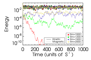
In figure 1, we plot the time history of the kinetic and magnetic energies for runs with resolution $32\times 64\times 32$. We identify three distinct regimes: (1) $Re<Re_{\text{crit}}$: the flow remains largely laminar and the initial perturbations die off, (2) $Re>Re_{\text{crit}}$ but $Rm<Rm_{\text{crit}}$: kinetic energy grows and sustains for sometime while the magnetic energy decays immediately after reaching the saturation state, (3) $Re>Re_{\text{crit}}$ and $Rm>Rm_{\text{crit}}$: Both kinetic and magnetic energy sustain growth. Fig. 1 shows that $Rm_{\text{crit}}\sim 1,200$. We estimated $Re_{\text{crit}}\sim 750$ for both hydrodynamic and MHD runs, which is consistent with the value found in the hydrodynamic simulations of PCF Manneville (2015) (note that the definition typically used in PCF literature is a factor of 2 smaller than our definition). These critical values have also been verified at a higher resolution of $64\times 128\times 64$. Note that the finite lifetime of turbulence as seen in the kinetic energy of $Re=Rm=1,000$ (red) run in fig. 1 is consistent with what has recently been found in hydrodynamic shear flow experiments Hof et al. (2006). Ref. Manneville (2015) suggests that turbulence in linear shear flows in small domains ($L_{y},L_{z}\sim L_{x}$) exhibit transient chaos, while large aspect ratio domains $L_{y},L_{z}\gg L_{x}$ would instead abruptly transition into steady turbulence. We do not explore extended domains herein so our results would represent a lower limit on the robustness of turbulence.

Figure 2: Same as 1 for $1\times 2\times 1$ (red, middle two lines), $1\times 2\times 4$ (green, top two lines), $4\times 8\times 4$ (blue, bottom two lines) at $Rm=10,000$.

II.2 Domain Size effects

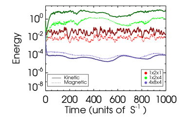
We plot the ratio of kinetic energy to magnetic energy in fig. 2 for three different domain sizes (see table 1 for description) $1\times 2\times 1$ ($64^{3}$), $1\times 2\times 4$ ($64\times 64\times 256$) and $4\times 8\times 4$ ($256^{3}$). The table also has data for a higher resolution run for the domain $1\times 2\times 1$, which suggests convergence for this aspect ratio. The magnetic energy is nearly an order of magnitude smaller than kinetic energy in $1\times 2\times 1$ and $1\times 2\times 4$ whereas in the the largest domain, $4\times 8\times 4$ the two are nearly equal. For the range of domains studied so far, this energy ratio therefore depends not only on the aspect ratio $L_{z}/L_{x}$ but increases with box size for a fixed aspect ratio.

Domain Size	Resolution	$\frac{\overline{[B^{2}]}}{\overline{[V^{2}]}}$	$\frac{\overline{\partial{\langle\mathcal{E}_{x}\rangle}/\partial z}^{z+}}{\overline{\langle SB_{x}\rangle}^{z+}}$	Rm
$1\times 2\times 1$	$64\times 64\times 64$	$0.204$	$0.017$	$10,000$
$1\times 2\times 1$	$128\times 128\times 128$	$0.211$	$0.007$	$10,000$
$1\times 2\times 4$	$64\times 64\times 256$	$0.062$	$0.002$	$10,000$
$4\times 8\times 4$	$256\times 256\times 256$	$2.413$	$0.011$	$40,000$

Table 1: Description of the three runs analyzed herein, with one higher resolution run done for convergence test. The third column is the ratio of magnetic to kinetic energies $\overline{[B^{2}]}/\overline{[V^{2}]}$ while the fourth column shows that the shear dominates the EMF derivative term $\partial{\overline{\langle\mathcal{E}_{x}\rangle}}/\partial z$ in the induction equation for the y-component of the magnetic field ($[Q]=$ volume average of $Q$, $\overline{Q}=$ time average of $Q$ from $100S^{-1}$ to $200S^{-1}$, $Q^{z+}$ represents the vertical average from $z=0$ to $z=+L_{z}/2$, and $xy$ average of Q is represented by $\langle Q\rangle$.). The last column lists the magnetic Reynolds number for the three different runs.

Figure 3: $xy$ averaged $\langle V_{x}\rangle$, $\langle V_{y}\rangle$, $\langle B_{x}\rangle$ and $\langle B_{y}\rangle$ for the run $1\times 2\times 1$ for the first $1000$ shear times. The x-axis is the time ($1/S$ units) and the y-axis is the vertical domain size in $L$ units.

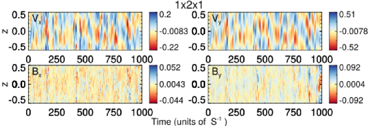
The velocity profiles $\langle V_{x}\rangle$, $\langle V_{y}\rangle$ and the magnetic field profiles $\langle B_{x}\rangle$, $\langle B_{y}\rangle$ averaged over $xy$ are plotted for the run with $1\times 2\times 1$ domain in fig. 3. Unlike the magnetic fields, we see that while the velocities are dominated by a sinusoidal profile in ‘z’ that varies in time. Furthermore, the $\langle B_{x}\rangle$ profile is more noisy than $\langle B_{y}\rangle$. The simulation began with a shear profile ${\bm{V}}_{\text{sh}}=-Sx{\bm{e}}_{y}$, and eventually reached a steady state with additional shear in the $z-$direction for the $xy$ averaged velocity fields, $\langle\bm{V}\rangle_{\text{ver. sh}}\sim\sin k_{z}z({\bm{e}}_{x}+{\bm{e}}_{y})$. This structure is a generic feature of hydrodynamic shear flows at and just above $Re_{\text{crit}}$. Recent work on the transition to turbulence suggests that as the domain size and $Re$ are increased, these structures disappear into ‘featureless’ turbulence Manneville (2015); Barkley and Tuckerman (2005).

Figure 4: $xy$ averaged $\langle B_{x}\rangle$ and $\langle B_{y}\rangle$ for the runs $1\times 2\times 4$ (left column) and $4\times 8\times 4$ (right column) for the first $1000$ shear times. The x-axis is in the units of $1/S$, while the y-axis represents the vertical domain in $L$ units. Note a strong anti-correlation between the $\langle B_{x}\rangle$ and $\langle B_{y}\rangle$ for both runs.

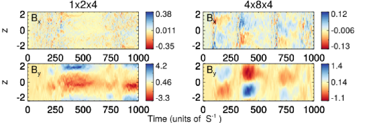
To explore possible generation of an organized magnetic field, we plot the magnetic field profiles for the two larger domains with $L_{z}=4$: $1\times 2\times 4$ and $4\times 8\times 4$ in fig. 4. The ‘y’ component of the magnetic field, $\langle B_{y}\rangle$ seems to be very coherent in both runs and $\langle B_{x}\rangle$ in the $4\times 8\times 4$ run displays considerable large scale organization compared to the corresponding plot for $1\times 2\times 4$. The magnetic fields are strongly correlated with the velocity fields (see Appendix) for $4\times 8\times 4$ since all of them have sinusoidal structure on the box scale. More interestingly, the magnetic to kinetic energy ratio is nearly unity (see table 1). This is in contrast to the $1\times 2\times 4$ run where the magnetic energy is more than an order of magnitude smaller than the kinetic energy and the $\langle B_{x}\rangle$ profile seems to be very noisy. The cross helicity of the $1\times 2\times 4$ run is close to unity for a significant duration, while that of $4\times 8\times 4$ is smaller in comparison and fluctuates about zero suggesting that the $1\times 2\times 4$ run is dominated by $k_{z}=1$ mode (see Appendix for plots).

The spatiotemporal profile of $\langle B_{y}\rangle$ in fig. 4 suggests the existence of a cycle period and thus a large scale dynamo. In the $xy$ averaged induction equation:

$$\frac{\partial\langle B_{x}\rangle}{\partial t} =-\frac{\partial}{\partial z}\langle V_{z}^{\prime}B_{x}^{\prime}-V_{x}^{\prime}B_{z}^{\prime}\rangle+\eta\frac{\partial^{2}}{\partial z^{2}}\langle B_{x}\rangle$$

$$\frac{\partial\langle B_{y}\rangle}{\partial t} =S\langle B_{x}\rangle+\frac{\partial}{\partial z}\langle V_{y}^{\prime}B_{z}^{\prime}-V_{z}^{\prime}B_{y}^{\prime}\rangle+\eta\frac{\partial^{2}}{\partial z^{2}}\langle B_{y}\rangle$$ (3)

the only terms that can contribute to the right side of the $\langle B_{y}\rangle$ equation are the EMF term $\partial_{z}\langle\mathcal{E}_{x}\rangle$ (where $\langle\bm{\mathcal{E}}\rangle=\langle\bm{V^{\prime}}\times\bm{B^{\prime}}\rangle$, $V^{\prime}$ and $B^{\prime}$ are fluctuations resulting from $xy$ averaging) and the ‘Omega’ term $S\langle B_{x}\rangle$ as seen in eq. 3 (the mean field term contribution, $\partial(\langle V\rangle\times\langle B\rangle)_{i}/\partial z\sim 0$, where $i=x,y$). We estimated the former to be roughly two orders of magnitude smaller than the shear term (table 1)

Figure 5: Power spectra of $xy$ averaged azimuthal velocity $\langle V_{y}\rangle$ and magnetic field $\langle B_{y}\rangle$ averaged from $501$ to $600$ shear times as a function of $k_{z}$ (in units of $(2\pi n_{z}/L_{z})$). The top (green) two lines represent $1\times 2\times 4$, while the middle (red) two represent $1\times 2\times 1$ and $4\times 8\times 4$ (blue) lines are at the bottom. The power spectra are normalized such that $\sum_{k_{z}}|\langle Q\rangle(k_{z})|^{2}=[Q^{2}]$.

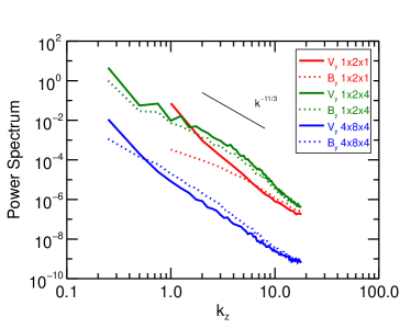
We plot the power spectra of the velocity and magnetic field averaged over $xy$ and Fourier transformed in ‘z’ in fig. 5. The predominance of the $k_{z}=1$ (in units of $(2\pi n_{z}/L_{z})$) mode is consistent with the nearly sinusoidal profile of $\langle V_{y}\rangle$ seen in fig. 3 and $\langle B_{y}\rangle$ in 4. The velocity spectrum for $1\times 2\times 4$ seems to follow the 1D Kolmogorov scaling $k^{-11/3}$ for intermediate wavemodes, which would imply that these modes represent the inertial range. However, the velocity power spectrum peaks at the box scale, which could be due to strong 2D vortex structures Xia et al. (2011). The velocity structures in the smallest domain $1\times 2\times 1$ do not seem to follow the 1D Kolmogorov scaling, while the largest domain $4\times 8\times 4$ has a steeper power law behavior for the most part but appears to have a flatter power law spectrum closer to the dissipation scale.

Since the velocity fields are dominated by box scale structures, it becomes a subtle matter to define and distinguish small vs. large scale dynamos Ebrahimi and Blackman (2016) or system scale dynamo Tobias et al. (2011). An additional caveat is that we are using periodic boundaries and thus the large power observed in box scale structures is an indication that the boundary conditions are strongly influencing the flow dynamics. It remains to be explored whether magnetic fields in such high $Re$ turbulent flows with a featureless velocity profile would show large scale organization. We do note that recent analytic theory for large scale field growth in shearing boxes shows that rotation is not necessary for dynamo action when a source of velocity fluctuations is present in a shear flow Ebrahimi and Blackman (2016). Our simulations satisfy their minimum sufficient conditions, although we focus on $xy$ averaging rather than the $yz$ averaging of their case.

III Conclusions

Using high resolution 3-D simulations of a shearing box with a pseudospectral code, we have demonstrated numerically for the first time that not only does shear driven turbulence sustain for high enough $Re$, but this turbulence amplifies and sustains magnetic energy when $Rm$ is large enough. This contrasts the work of Ref. Hawley et al. (1996) who did not identify sustained growth in magnetic energy because their $Rm$ was below the critical value we have found. The turbulence emergent in our simulations is self-sustained by the linear shear and thus distinct from a different class of work that employed stochastic forcing in addition to the non-rotating shear Yousef et al. (2008); Sridhar and Subramanian (2009); Shapovalov and Vishniac (2011); Tobias and Cattaneo (2013); Sridhar and Singh (2014); Squire and Bhattacharjee (2015a, b). Structures in both velocity and magnetic fields at the largest scales are seen in our largest domains and we have identified the EMF terms that sustain the latter. Whether the velocity structures break into featureless turbulence at even higher Reynolds numbers and domain sizes remains to be explored, but the minimum ingredients derived for large scale field growth Ebrahimi and Blackman (2016) are met.

Acknolwedgements:-

We thank F. Ebrahimi, P. Bhat, and S. Tobias for related discussions. The simulations reported on in this paper were done on the Blue Streak cluster hosted by the Center for Integrated Research Computing at the University of Rochester. FN acknowledges funding from the European Research Council under the European Union’s Seventh Framework Programme (FP/2007-2013) under ERC grant agreement 306614. EB acknowledges support from grants HST-AR-13916.002 and NSF-AST1515648.

IV Appendix

Figure 6: Time evolution of horizontally averaged cross helicity $\langle{\bf v}\cdot{\bf b}\rangle^{z+}$ vertically averaged from $z=0$ to $z=+L_{z}/2$ plotted for $1\times 2\times 1$ (red, solid), $1\times 2\times 4$ (green, dashed), $4\times 8\times 4$ (blue, dotted) for the first $1000S^{-1}$.

Figure 7: Same as fig. 6 but for $\langle{\bf v}\cdot{\bf b}\rangle^{z-}$ vertically averaged from $z=-L_{z}/2$ to $z=0$.

Figure 8: Same as fig. 6 but for $[{\bf v}\cdot{\bf b}]$ volume averaged.

Figure 9: $xy$ averaged $\langle V_{x}\rangle$ and $\langle V_{y}\rangle$ for the runs $1\times 2\times 4$ (left column) and $4\times 8\times 4$ (right column) for the first $1000$ shear times. Compare fig. 4 from the main paper.

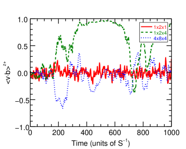
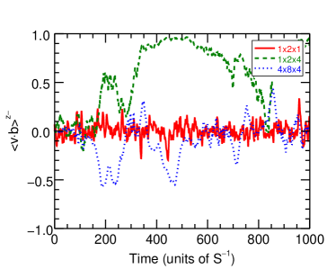
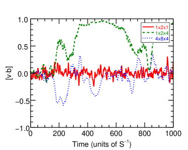
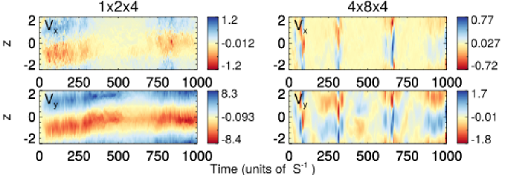
We plot the cross helicity averaged from $z=0$ to $z=+L_{z}/2$ represented by $\langle{\bf v}\cdot{\bf b}\rangle^{z+}$ ($\langle{\bf v}\cdot{\bf b}\rangle^{z-}$: $z=-L_{z}/2$ to $z=0$; $[{\bf v}\cdot{\bf b}]$: volume average) for the three runs in figs. 6, 7, 8. It appears that the $1\times 2\times 4$ run has a cross helicity dominated by the largest mode and thus has nearly maximal cross helicity with the same sign for different vertical sections of the box for a considerable duration of time. This is further supported by the velocity profiles of this run that are also attached in fig. 9. The velocity profiles for this run are all seemingly locked into $k_{z}=1$ state, similar to the magnetic field profiles in fig. 4 of the main text. Of the 3 runs, the $1\times 2\times 4$ is the only one with a dominant vertical extent ($L_{z}/L_{x}>1$). The large vertical extent seems to be required for the appearance of this large scale dominant mode.

References

- Liang et al. (2013) E. Liang, M. Boettcher, and I. Smith, ApJL 766, L19 (2013), arXiv:1111.3326 [astro-ph.HE] .
- Miesch and Toomre (2009) M. S. Miesch and J. Toomre, Annual Review of Fluid Mechanics 41, 317 (2009).
- Brüggen and Vazza (2015) M. Brüggen and F. Vazza, in Magnetic Fields in Diffuse Media, Astrophysics and Space Science Library, Vol. 407, edited by A. Lazarian, E. M. de Gouveia Dal Pino, and C. Melioli (2015) p. 599.
- Cally (2000) P. S. Cally, Sol. Phys. 194, 189 (2000).
- Brandenburg et al. (2012) A. Brandenburg, D. Sokoloff, and K. Subramanian, Space Sci. Rev. 169, 123 (2012), arXiv:1203.6195 [astro-ph.SR] .
- Mamatsashvili et al. (2014) G. R. Mamatsashvili, D. Z. Gogichaishvili, G. D. Chagelishvili, and W. Horton, Phys. Rev. E 89, 043101 (2014), arXiv:1409.8543 [physics.plasm-ph] .
- Manneville (2015) P. Manneville, European Journal of Mechanics - B/Fluids 49, Part B, 345 (2015), trends in Hydrodynamic Instability in honour of Patrick Huerre’s 65th birthday.
- Mullin (2011) T. Mullin, Annual Review of Fluid Mechanics 43, 1 (2011), http://dx.doi.org/10.1146/annurev-fluid-122109-160652 .
- Hawley et al. (1996) J. F. Hawley, C. F. Gammie, and S. A. Balbus, Astrophys. J. 464, 690 (1996).
- Shakura and Postnov (2015) N. Shakura and K. Postnov, MNRAS 448, 3697 (2015), arXiv:1412.1223 [astro-ph.HE] .
- Velikhov (1959) E. P. Velikhov, JETP 36, 995 (1959).
- Chandrasekhar (1960) S. Chandrasekhar, Proceedings of the National Academy of Science 46, 253 (1960).
- Balbus and Hawley (1991) S. A. Balbus and J. F. Hawley, Astrophys. J. 376, 214 (1991).
- Blackman and Nauman (2015) E. G. Blackman and F. Nauman, Journal of Plasma Physics 81, 395810505 (2015), arXiv:1501.00291 [astro-ph.HE] .
- Schekochihin et al. (2004) A. A. Schekochihin, S. C. Cowley, S. F. Taylor, J. L. Maron, and J. C. McWilliams, Astrophys. J. 612, 276 (2004), astro-ph/0312046 .
- Haugen et al. (2004) N. E. Haugen, A. Brandenburg, and W. Dobler, Phys. Rev. E 70, 016308 (2004), astro-ph/0307059 .
- Yousef et al. (2008) T. A. Yousef, T. Heinemann, A. A. Schekochihin, N. Kleeorin, I. Rogachevskii, A. B. Iskakov, S. C. Cowley, and J. C. McWilliams, Physical Review Letters 100, 184501 (2008), arXiv:0710.3359 .
- Sridhar and Subramanian (2009) S. Sridhar and K. Subramanian, Phys. Rev. E 79, 045305 (2009), arXiv:0812.3269 .
- Shapovalov and Vishniac (2011) D. S. Shapovalov and E. T. Vishniac, Astrophys. J. 738, 66 (2011).
- Tobias and Cattaneo (2013) S. M. Tobias and F. Cattaneo, Nature (London) 497, 463 (2013).
- Sridhar and Singh (2014) S. Sridhar and N. K. Singh, MNRAS 445, 3770 (2014), arXiv:1306.2495 .
- Squire and Bhattacharjee (2015a) J. Squire and A. Bhattacharjee, Physical Review Letters 115, 175003 (2015a), arXiv:1506.04109 [astro-ph.SR] .
- Squire and Bhattacharjee (2015b) J. Squire and A. Bhattacharjee, Astrophys. J. 813, 52 (2015b), arXiv:1507.03154 [astro-ph.HE] .
- Note (1) http://ipag.osug.fr/~lesurg/snoopy.html.
- Lesur and Longaretti (2011) G. Lesur and P.-Y. Longaretti, A&A 528, A17 (2011), arXiv:1012.2690 [astro-ph.EP] .
- Note (2) We do not conduct a detailed study on the critical amplitude required to trigger and sustain turbulence and simply use velocity perturbations of amplitude for all of our simulations.
- Hof et al. (2006) B. Hof, J. Westerweel, T. M. Schneider, and B. Eckhardt, Nature (London) 443, 59 (2006).
- Barkley and Tuckerman (2005) D. Barkley and L. S. Tuckerman, Physical Review Letters 94, 014502 (2005), physics/0403142 .
- Xia et al. (2011) H. Xia, D. Byrne, G. Falkovich, and M. Shats, Nature Physics 7, 321 (2011).
- Ebrahimi and Blackman (2016) F. Ebrahimi and E. G. Blackman, MNRAS 459, 1422 (2016), arXiv:1509.04572 [astro-ph.HE] .
- Tobias et al. (2011) S. M. Tobias, F. Cattaneo, and N. H. Brummell, The Astrophysical Journal 728, 153 (2011).