Millisecond radio pulsars with known masses: parameter values and equation of state models

Abstract

The recent fast growth of a population of millisecond pulsars with precisely measured mass provides an excellent opportunity to characterize these compact stars at an unprecedented level. This is because the stellar parameter values can be accurately computed for known mass and spin rate and an assumed equation of state (EoS) model. For each of the 16 such pulsars and for a set of EoS models from nucleonic, hyperonic, strange quark matter and hybrid classes, we numerically compute fast spinning stable stellar parameter values considering the full effect of general relativity. This first detailed catalogue of the computed parameter values of observed millisecond pulsars provides a testbed to probe the physics of compact stars, including their formation, evolution and EoS. We estimate uncertainties on these computed values from the uncertainty of the measured mass, which could be useful to quantitatively constrain EoS models. We note that the largest value of the central density $\rho_{\rm c}$ in our catalogue is $\sim 5.8$ times the nuclear saturation density $\rho_{\rm sat}$, which is much less than the expected maximum value $13\rho_{\rm sat}$. We argue that the $\rho_{\rm c}$-values of at most a small fraction of compact stars could be much larger than $5.8\rho_{\rm sat}$. Besides, we find that the constraints on EoS models from accurate radius measurements could be significantly biased for some of our pulsars, if stellar spinning configurations are not used to compute the theoretical radius values.

1 Introduction

Compact stars, commonly known as “neutron stars”, are possibly the densest objects in the universe apart from black holes. A class of such compact stars, pulsars, show periodic variation of intensity in their electromagnetic emission. In fact, compact stars were discovered from such periodic radio pulses (Hewish et al., 1968). The first reported fast spinning pulsar, i.e., the millisecond (ms) pulsar, was PSR B1937+21 (Backer et al., 1982). It was immediately proposed that such pulsars could be spun up by accretion-induced angular momentum transfer in low-mass X-ray binaries (LMXBs; Radhakrishnan & Srinivasan, 1982; Alpar et al., 1982). This model was strengthened by the discovery of an accretion-powered X-ray ms pulsar SAX J1808.4-3658 (Wijnands & van der Klis, 1998; Chakrabarty & Morgan, 1998). This is because this X-ray pulsar showed that compact stars could be spun up in LMXBs. However, a clear evolutionary connection between radio ms pulsars and LMXBs would be established if a compact star had shown both LMXB phase and radio pulsations possibly in a non-accreting phase. Recently, three such sources, called transitional pulsars, have been discovered (Archibald et al., 2009; Papitto et al., 2013; de Martino et al., 2013). These findings strongly show that ms pulsars are spun up in LMXBs. However, the detailed mechanism of this spin evolution, which depends on accretion processes and the interaction between the accretion disc and the stellar magnetosphere, is somewhat poorly understood. Testing the models of these physical processes against the precisely measured parameter values of observed ms pulsars will be very useful to understand the physics of compact star evolution.

Another poorly understood aspect of compact stars is their internal composition, especially the physics of their cores. The densities of these degenerate cores are well above the nuclear saturation density $\rho_{\rm sat}\approx 2.6\times 10^{14}$ g cm^-3. Consequently (see, e.g., Bombaci, 2007) various particle species (apart from neutrons, protons, electrons and muons) and phases of dense matter are expected in the stellar interior. Thus different types of compact stars (nucleonic, hyperonic, strange matter, hybrid) are hypothesized to exist. Therefore compact stars can be considered as natural laboratories that allow us to investigate the constituents of matter and their interactions under extreme conditions that cannot be reproduced in any terrestrial laboratory. Understanding the nature of supra-nuclear core matter remains a fundamental problem of physics, even after almost 50 years since the discovery of the first pulsar.

The standard way attempted to solve this problem is the following. Assuming the constituents of the stellar matter and the interactions among them, an equation of state (EoS) is computed using different many-body approaches. The EoS is given by the thermodynamical relation between the matter pressure $P$, the mass density $\rho$ and the temperature $T$. The temperature could be considered equal to zero a few minutes after the compact star birth (Burrows & Lattimer, 1986; Bombaci et al., 1995; Prakash et al., 1997). Many such EoS models exist in the literature.

In order to understand the superdense matter of compact star cores, it is required to identify the “correct” EoS model. How can one do that? For a proposed EoS model, one can compute the stable stellar structure. For doing this, one needs to solve the Tolman-Oppenheimer-Volkoff (TOV) equations (Oppenheimer & Volkoff, 1939; Tolman, 1939) for nonspinning compact stars. For fast spinning stars, however, one needs to follow a numerical formalism described and used in this paper. Once the stable stellar structure is computed, it is possible to calculate the values of various stellar parameters, such as mass, radius, spin rate, etc. One needs to compare these computed values with the measured values to reject some proposed EoS models. By rejection of many EoS models, one can attempt to identify the “correct” EoS model as accurately as possible. In order to achieve this goal, one needs to measure three independent parameters of the same ms pulsar.

So far, for no compact star three parameters have been precisely measured. However, precise measurements of two parameters, mass and spin rate, have been done for a fast growing population of ms pulsars in recent years. This, for the first time, provides a unique opportunity to characterize a number of observed ms pulsars with an unprecedented accuracy. Note that previous authors explored the stable structure of compact stars, which provided general information about the fast spinning compact star parameters (e.g., Cook et al., 1994). Some authors went a step further, considered the measured spin rate of an ms pulsar, and computed a constant spin sequence for that pulsar (e.g., Datta et al., 1998; Bhattacharyya et al., 2016). But such a sequence gives large ranges of other parameter values for a given EoS model. Therefore, while this sequence gives an insight about the general properties of ms pulsars, it does not give very useful additional information about the parameters of the considered ms pulsar. Furthermore, since these large ranges of parameter values overlap for various EoS models, such spin sequences are not very useful to constrain EoS models. With two parameters known, we can now accurately estimate the other parameter values of observed ms pulsars for a given EoS model. In this paper, we do this estimation for 16 ms pulsars and eight diverse EoS models from four different classes, and make a catalogue. This catalogue not only will be useful to constrain EoS models, but also will provide a testbed to probe the physical processes of compact star evolution. We also discuss the ways to constrain EoS models using measured radius values.

In § 2, we mention and discuss the ms pulsars and EoS models we consider. In § 3, we describe the procedure to compute stable fast spinning compact star structure. § 4 includes our catalogue of computed ms pulsar parameters and a detailed discussion on their implications. In § 5, we summarize our results and conclusions.

2 Pulsars and equations of state

As mentioned in § 1, in this work we use a special sample of ms pulsars, that is those with precisely measured mass values. Here we define pulsars with spin periods less than 10 ms as ms pulsars. Masses of these pulsars in binary stellar systems were measured from the estimation of post-Keplerian parameters or the spectroscopic observations of the companion white dwarf stars (see Özel & Freire (2016) and references therein). We choose ms pulsars with quoted mass error less than a quarter of a solar mass. We list the spin rates, measured masses with errors and the references on spin and mass measurements for these pulsars in Table 1. It is interesting to see that masses of all these pulsars are distributed within the $1-2M_{\odot}$ range.

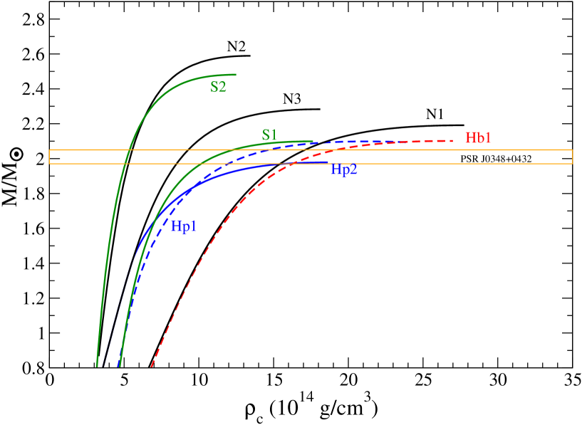
Figure 2: Compact star gravitational mass versus central density curves. Eight curves for non-spinning stars (§ 3) are for eight EoS models (marked by names given in Table 2). The horizontal lines show the mass ($2.01\pm 0.04M_{\odot}$) of the relatively slowly spinning (spin period $=39$ ms) pulsar PSR J0348+0432.

In this paper, we consider eight EoS models from four different classes (Table 2). We carefully chose these EoS models keeping various points in mind. For example, three of our EoS models are nucleonic, two are hyperonic, two are strange quark matter and one is hybrid, and hence the set is truly diverse. Moreover, the discovery of the massive pulsar PSR J0348+0432 with a precisely measured mass ($2.01\pm 0.04M_{\odot}$; Antoniadis et al. (2013)) demands that the “correct” EoS must be able to support this high mass. All our EoS models pass this test (Figs. 1, 2 and Table 2). We also note that the discoveries of this pulsar and another massive pulsar (PSR J1614-2230; Demorest et al. (2010); see also Table 1) essentially constrained the radius space from the lower side. This is because, within a certain class of EoS models (e.g., nucleonic or strange matter), a harder EoS which can support a higher maximum mass gives a higher radius value for a given mass (see Fig. 1). Therefore, as indicated by this figure, EoS models with radius values less than a certain limit in the observed $1-2M_{\odot}$ mass range (Table 1) may not be able to support the high mass values of PSR J0348+0432 and PSR J1614-2230, thus effectively shrinking the radius space. Our EoS models nicely fill this shrunken radius space (see Fig. 1).

Here we give a brief description for each EoS model.
(1) Nucleonic matter: The first nucleonic EoS model (N1), denoted by A18+$\delta v$+UIX (Akmal et al. (1998); Table 2), is based on the Argonne $v_{18}$ model A18 (Wiringa et al., 1995) of two-nucleon interaction. The A18 model fits very well the phase shifts for nucleon-nucleon scattering of the Nijmegen database (Stoks et al., 1993). The A18+$\delta v$+UIX model additionally includes three-nucleon interactions described by the Urbana IX [UIX] model (Pudliner et al., 1995) and the effect of relativistic boost corrections. The second nucleonic EoS model (N2; Sahu et al. (1993); Table 2), which is harder (§ 1) than N1, is a field theoretical EoS for nucleonic matter in $\beta$-equilibrium based on the chiral sigma model. The model includes an isoscalar vector field generated dynamically. The third nucleonic EoS model (N3; Sugahara & Toki (1994); Providencia & Rabhi (2013); Table 2) is based on a relativistic mean field (RMF) approach in which nucleons ($n$, $p$) interact via the exchange of $\sigma$, $\omega$ and $\rho$ mesons. In particular, in the present work we use the parameters set denoted as TM1-2 in Table I of Providencia & Rabhi (2013). All the nucleonic EoS models used in our calculations reproduce the empirical saturation point of nuclear matter $n_{sat}=0.16\pm 0.01~{}{\rm fm}^{-3}$, $E/A|_{n_{sat}}=-16.0\pm 1.0~{}{\rm MeV}$ (e.g., Logoteta et al., 2015) and the empirical value of the nuclear symmetry energy $E_{sym}(n_{sat})=28$ – $33$ MeV, at saturation density.
(2) Hyperonic matter: The first hyperonic EoS model (Hp1; Banik et al., 2014) is based on a RMF approach in which nucleons and $\Lambda$ hyperons interact via the exchange of $\sigma$, $\omega$ and $\rho$ mesons with the additional contribution of the hidden-strangeness meson $\phi(1020)$ and using density dependent coupling constant. The second hyperonic EoS model (Hp2; Providencia & Rabhi, 2013) is also based on a RMF approach, which includes all the members of the $J^{\pi}=(1/2)^{+}$ baryon octet (i.e. $n$, $p$, $\Lambda$, $\Sigma^{-}$, $\Sigma^{0}$, $\Sigma^{+}$, $\Xi^{-}$ and $\Xi^{0}$) interacting via $\sigma$, $\omega$, $\rho$ and hidden-strangeness $\sigma^{*}$ and $\phi(1020)$ meson exchange. Among the different hyperonic EoS parametrizations reported in Providencia & Rabhi (2013), in the present work we use the one corresponding to the TM1-2 parameters set for the nucleonic sector, without $\sigma^{*}$ mesons, with $\Lambda_{\omega}=0$ and taking for the potential energy depths for the $\Lambda$, $\Sigma$, and $\Xi$ hyperons in symmetric nuclear matter at saturation density $n_{\rm sat}$ with the values $U_{\Lambda}=-28~{}{\rm MeV}$, $U_{\Sigma}=30~{}{\rm MeV}$, $U_{\Xi}=18~{}{\rm MeV}$ respectively (see Table II in Providencia & Rabhi, 2013).
(3) Strange quark matter: These EoS models are the simple version of the MIT bag model, which was extended to include perturbative corrections due to quark interactions, up to the second order in the strong structure constant (Fraga et al., 2001; Alford et al., 2005; Weissenborn et al., 2011). These EoS models are characterized with two parameters: effective bag constant ($B_{\rm eff}$) and perturbative QCD corrections term parameter ($a_{4}$). The value $a_{4}=1$ corresponds to the ideal relativistic Fermi gas EoS. For the first model (S1), $B_{\rm eff}^{1/4}=138$ MeV, $a_{4}=0.8$, while for the second model (S2), $B_{\rm eff}^{1/4}=125$ MeV, $a_{4}=0.5$ (Bhattacharyya et al., 2016). Note that S2 is harder (§ 1) than S1.
(4) Hybrid (nuclear+quark) matter: In this class of models, one assumes the occurence of the quark deconfinement phase transition in the neutron star core. Following Glendenning (1992, 1996), we model the nuclear to quark matter transition as a first order phase transition occuring in a multicomponent system with two conserved “charges” (the electric charge and the baryon number). The specific hybrid star matter EoS model (Hb1) considered in the present paper, has been obtained using the A18+$\delta v$+UIX EoS (Akmal et al., 1998) for the nuclear matter phase and the extended MIT bag model EoS (Fraga et al., 2001; Alford et al., 2005; Weissenborn et al., 2011) for the quark phase with $B_{\rm eff}^{1/4}=138$ MeV, $a_{4}=0.4$.

3 Fast spinning stellar structure computation

Here we briefly mention the method to compute fast spinning stable compact star structures, the corresponding stellar parameters and the equilibrium sequences. A detailed description of the method can be found in Cook et al. (1994). Such computation requires a general relativistic treatment. The general spacetime of such a star is (using $c=G=1$; Bardeen (1970); Cook et al. (1994)):

$${\rm d}s^{2}=-{\rm e}^{\gamma+\rho}{\rm d}t^{2}+{\rm e}^{2\alpha}({\rm d}r^{2}+r^{2}{\rm d}\theta^{2})+{\rm e}^{\gamma-\rho}r^{2}\sin^{2}\theta$$

$$({\rm d}\phi-\omega{\rm d}t)^{2},$$ (1)

where $t$, $r$ and $\theta$ are temporal, quasi-isotropic radial and polar angular coordinates respectively, $\gamma$, $\rho$, $\alpha$ are metric potentials, and $\omega$ is the angular speed of the stellar fluid relative to the local inertial frame. Einstein’s field equations are solved to compute the $r$ and $\theta$ dependent $\gamma$, $\rho$, $\alpha$ and $\omega$, as well as the stable stellar structure, for a given EoS model, and assumed values of two parameters, such as stellar central density ($\rho_{\rm c}$) and polar radius to equatorial radius ratio (Cook et al., 1994; Datta et al., 1998; Bombaci et al., 2000; Bhattacharyya et al., 2000, 2001a, 2001b, 2001c; Bhattacharyya, 2002, 2011). This equilibrium solution is then used to compute compact star parameters, such as gravitational mass ($M_{\rm G}$), rest mass ($M_{\rm 0}$), equatorial circumferential radius ($R_{\rm e}$), spin frequency ($\nu$), total angular momentum ($J$), moment of inertia ($I$), total spinning kinetic energy ($T$) and total gravitational energy ($W$) (Cook et al., 1994; Datta et al., 1998).

The radius $r_{\rm ISCO}$ of the innermost stable circular orbit (ISCO) is calculated in the following way. The radial equation of motion around such a compact star is ṙ${}^{2}\equiv{\rm e}^{2\alpha+\gamma+\rho}({\rm d}r/{\rm d}\tau)^{2}=$Ẽ${}^{2}-$Ṽ², where, ${\rm d}\tau$ is the proper time, Ẽ is the specific energy, which is a constant of motion, and Ṽ is the effective potential. The effective potential is given by Ṽ${}^{2}={\rm e}^{\gamma+\rho}[1+\frac{l^{2}/r^{2}}{{\rm e}^{\gamma-\rho}}]+2\omega$Ẽ$l-\omega^{2}l^{2}$. Here $l$ is the specific angular momentum and a constant of motion. We determine $r_{\rm ISCO}$ using the condition Ṽ_,rr = 0, where a comma followed by one $r$ represents a first-order partial derivative with respect to $r$ and so on (Thampan and Datta, 1998).

We compute the static or nonspinning limit, where $\nu\rightarrow 0$ and $J\rightarrow 0$, for all EoS models (see Figs. 1 and 2). The main aim of this paper is to compute various parameter values of all the 16 pulsars mentioned in Table 1. We obtain the stable configuration for known mass and spin rate of each ms pulsar and for each EoS model using multi-iteration runs of our numerical code. Such multi-iteration runs include computations of the constant $\nu$ equilibrium sequence. Then various parameter values describing this equilibrium configuration are obtained. It is also useful to obtain the uncertainties in these parameters. Note that measurement errors of $\nu$ values are sufficiently small (e.g., spin period $\sim 5.7574518191(9)$ ms for PSR J0437-4715; Johnston et al. (1993)). So the uncertainties of the computed parameters essentially come from the measurement errors of stellar mass values. These errors of $M_{\rm G}$ for each ms pulsar, as quoted in Table 1, give lower ($M_{\rm G}^{\rm l}$) and upper ($M_{\rm G}^{\rm u}$) mass values. We compute the two limits of each computed parameter for each pulsar and EoS model using $M_{\rm G}=M_{\rm G}^{\rm l}$ and $M_{\rm G}=M_{\rm G}^{\rm u}$ and the measured $\nu$. These two limits for a parameter give the uncertainties quoted in Table 3.

4 Results and discussion

4.1 Properties of millisecond pulsars

Here we present our results in Table 3, and discuss their implications. This table displays a catalogue of numerically computed parameter values of 16 ms pulsars (from Table 1) with precisely measured mass. For each pulsar, we calculate parameter values with error bars for each of eight EoS models (Table 2), using the procedure mentioned in § 3.

Since we compute stellar parameter values for diverse EoS models, the numbers given in Table 3 characterize observed ms pulsars at an unprecedented level. Moreover, since our sample pulsars have diverse mass and spin values, they may be representative enough for using this knowledge to understand other compact stars, including some of the fast spinning accreting stars in LMXBs. Therefore, the catalogue will provide a unique testbed to probe the physics of compact stars, including their formation, evolution and EoS, specifically for the 16 ms pulsars (Table 3). Below we discuss what we learn about a number of properties of these 16 ms pulsars, and their implications, based on detailed general relativistic computation of their structures using their measured masses and spin rates, and realistic EoS models.

(1) Central density ($\rho_{\rm c}$):

The central part of a compact star harbours possibly the densest matter in the universe, which is not hiding behind an event horizon. So it is tantalizing to know how dense this matter can be for observed compact stars, especially those with measured mass values. The knowledge of the range of this maximum density for compact stars with known masses should have impact on our understanding of constituents and physics of the dense matter. Such knowledge will also characterize the compact star populations, and will be important to understand their formation and evolution. This is because the $\rho_{\rm c}$-value at the birth is expected to depend on the astrophysical process related to the compact star formation. Moreover, this initial $\rho_{\rm c}$ evolves into our inferred $\rho_{\rm c}$-value, because ms pulsars acquire mass and angular momentum during their LMXB phases (e.g., Bejger et al., 2011).

The issue of the largest possible density $\rho_{\rm max}$ in compact stars has been previously investigated in Lattimer & Prakash (2005), where the authors report the calculated maximum mass ($M_{\rm G}^{\rm max}$) for non-spinning compact stars versus the corresponding central density for various EoS models. In addition, they make the conjecture that the analytic Tolman VII solution (Tolman, 1939) of the TOV equations marks the upper limit for the density reachable inside a compact star. The present accurate mass measurements for PSR J0348+0432 with $M=2.01\pm 0.04M_{\odot}$ (Antoniadis et al., 2013), using the argument of Lattimer & Prakash (2005) (see their Fig. 1), implies $\rho_{\rm max}\sim 13\rho_{\rm sat}$. Here, $\rho_{\rm sat}$ is the nuclear saturation density ($\approx 2.6\times 10^{14}$ g cm^-3). More recently, this argument has been also discussed in Lattimer & Prakash (2010), where the authors discuss also the limiting case of the so-called “maximally compact EoS” (Haensel & Zdunik, 1989); but again they get $\rho_{\rm max}\sim 13\rho_{\rm sat}$.

Table 3 displays the $\rho_{\rm c}$-ranges of 16 ms pulsars, each for eight EoS models. This table shows that a harder EoS model within an EoS class has a lower $\rho_{\rm c}$ for given gravitational mass ($M_{\rm G}$) and spin frequency ($\nu$) values. This is because the interaction between the stellar constituents is more repulsive for harder EoS models and hence it is more difficult to compress the matter. Here we note that, within the hyperonic class, Hp2 is harder below a certain density, and Hp1 is harder above this density. This could be possible because, while Hp1 includes only Lambda hyperons, Hp2 includes both Lambda and Sigma hyperons. This is why the $\rho_{\rm c}$ value is higher for Hp1 (compared to that for Hp2) except for the highest mass pulsar PSR J1614-2230 in Table 3. This table also shows that a more massive ms pulsar has higher $\rho_{\rm c}$ due to larger gravitational compression (compare, for example, the numbers for PSR J1946+3417 and PSR J1911-5958A, which have similar $\nu$ values).

Table 3 shows that the maximum $\rho_{\rm c}$-value for our sample of pulsars and our sample of diverse EoS models is $15.13_{-0.32}^{+0.34}\times 10^{14}$ g cm^-3 or $\approx 5.8_{-0.1}^{+0.1}\rho_{\rm sat}$. This value, which corresponds to the most massive pulsar (PSR J1614-2230) and a soft EoS model Hb1 of Table 3, is significantly lower than the currently believed highest possible $\rho_{\rm c}$-value ($\sim 13\rho_{\rm sat}$; Lattimer & Prakash (2005, 2010)). Can the $\rho_{\rm c}$-value of a compact star be much larger than the maximum value we find here? We discuss this point below.

Fig. 2 shows that the mass ($M_{\rm G}$) versus $\rho_{\rm c}$ curve for each EoS has a positive slope with two distinct parts: (1) one with high slope (almost vertical for harder EoS models), which occupies almost the entire mass range; and (2) one with low slope (almost horizontal), in which the $\rho_{\rm c}$-value significantly increases in a small mass range near the maximum mass that can be supported by a given EoS model. Now let us imagine an EoS model, which is the “correct” EoS model. This model cannot be much softer than the soft EoS models of our sample, because then it would not be able support the mass of the observed most massive pulsar (PSR J0348+0432; see Fig. 2). Therefore, Fig. 2 strongly suggests that the high-slope part of the $M_{\rm G}-\rho_{\rm c}$ curve of the “correct” EoS model cannot give a $\rho_{\rm c}$-value much larger than the maximum value ($\approx 5.8\rho_{\rm sat}$) we find here. The low-slope part for the “correct” EoS model could, however, provide a much larger $\rho_{\rm c}$-value. But since the low-slope part occupies a small mass range, only a small fraction of all compact stars, which have masses close to the maximum allowed mass, could have $\rho_{\rm c}$-values much larger than $5.8\rho_{\rm sat}$. However, if the “correct” EoS model is as hard as one of our harder EoS models (e.g., N2, S2), which can be confirmed if the mass of a more massive compact star is precisely measured in the future, then the $\rho_{\rm c}$-value of no compact star can be as high as $5.8\rho_{\rm sat}$. Therefore, we conclude that the $\rho_{\rm c}$-values of at most a small fraction of compact stars could be much larger than the maximum value we find here.

(2) Rest mass ($M_{0}$):

The rest mass (also referred to as baryonic mass) of a compact star is an important parameter. It can be written as $M_{0}=m_{u}N_{B}$, where $m_{u}=931.49$ MeV is the atomic mass unit and $N_{B}$ ($\sim$ a few $10^{57}$) is the total number of baryons in the star. For an isolated compact star, as a consequence of the baryon number conservation, $M_{0}$ is constant, whereas the corresponding values of the stellar gravitational mass $M_{G}$ and of the total stellar binding energy $B=M_{0}-M_{G}$ depend on the EoS (Bombaci & Datta, 2000) and on the stellar spin frequency. Thus, a non-accreting compact star evolves conserving its $M_{0}$ value (Cook et al., 1994).

The evolution of an accreting compact star depends on the binary properties and on the accretion processes which determine the accreted mass $\Delta M_{0}$ in a certain time span $\Delta t$. However, for a given accreted rest mass $\Delta M_{0}$, the increase $\Delta M_{\rm G}$ of the stellar gravitational mass will always be smaller than $\Delta M_{0}$ and will depend on the EoS. In fact, one has

$$\Delta M_{\rm G}=\Delta M_{0}-\Delta B<\Delta M_{0}\,,$$ (2)

where $\Delta B$ is the increase of the stellar binding energy due to accretion (Bagchi, 2011). This energy can be radiated by the system during the accretion stage not only as electromagnetic radiation (mostly X-rays), but also via neutrino emission, since the change in the total stellar rest mass due to accretion alters the $\beta$-equilibrium conditions in the stellar core.

One finds from Table 3 that strange matter EoS models have much higher $B$ values than nucleonic, hyperonic and hybrid EoS models. Besides, a softer EoS model has higher $B$ value than a harder EoS model within a class. We find $B$ in the range $\sim 0.1-0.5M_{\odot}$ for our sample of pulsars and EoS models. This is $\sim 7-30\%$ of the $M_{\rm G}$ values ($\sim 6-23\%$ of the $M_{0}$ values) of our sample pulsars, which is consistent with an upper limit of 25% of $M_{0}$ reported by Lattimer & Prakash (2010). This shows that a significant fraction of the accreted matter (rest-mass energy) was lost from the binary system via radiation, and via neutrino emission, for our 16 ms pulsars during their LMXB phases. This shows the importance of considering such loss of accreted matter in the modeling of binary evolution of these ms pulsars.

Since the effect of the total binding energy $B$ on the evolution of compact star spin rate and other properties is important, it is useful to have a simple relation between $M_{\rm G}$, $M_{0}$ and $J$ to compute the stellar spin evolution. Such a relation was proposed by Cipolletta et al. (2015) in their Eq. (20). A similar relation was earlier given by Eq. (93) of Prakash et al. (1997) for the total binding energy of non-spinning stars. We check that for our nucleonic, hyperonic and hybrid EoS models, the relation by Cipolletta et al. (2015) gives values consistent with 2% accuracy (as claimed by those authors), but the error is $\sim 6-12\%$ for our strange matter EoS models. This relation also usually works better for harder EoS models within a class.

(3) Radius and oblateness:

Attempts are being made for decades to measure the radii of compact stars using various spectroscopic and timing methods (e.g., van Paradijs, 1978; Gendre et al., 2003; Bhattacharyya et al., 2005; Bogdanov et al., 2007). Such a measurement is expected to be very useful to constrain EoS models. In Table 3, we list computed equatorial radius ($R_{\rm e}$) and polar radius ($R_{\rm p}$) values with errors of 16 ms pulsars for each of eight EoS models. These values can be used to constrain these models, if the radius of any of these pulsars is observationally estimated. Table 3 gives a radius range of $\approx 11-16$ km for all pulsars and EoS models, which implies that this is roughly the radius range which one needs to constrain. This range is consistent with previous findings (e.g., Hebeler et al., 2013). Besides, note that the knowledge of oblateness of a spinning compact star may be important to understand its physics, and to constrain its EoS models using various techniques (e.g., Miller & Lamb, 2015; Bauböck et al., 2013). The $R_{\rm p}/R_{\rm e}$ value, which determines the oblateness, decreases with increasing spin rate. For example, our fastest spinning pulsar has $R_{\rm p}/R_{\rm e}\approx 0.89$ for our hardest nucleonic EoS model, and our slowest spinning pulsar has $R_{\rm p}/R_{\rm e}$ value consistent with $1.00$ for the two strange matter EoS models (Table 3). This table gives an idea about typical $R_{\rm p}/R_{\rm e}$ values of our 16 ms pulsars, which can be incorporated in techniques to constrain EoS models.

(4) Radius-to-mass ratio ($R_{\rm e}/r_{\rm g}$):

Measurement of stellar radius-to-mass ratio, which is the inverse of stellar compactness, is an alternative to radius measurement for constraining EoS models. Here, $r_{\rm g}$ ($=GM_{\rm G}/c^{2}$) is the Schwarzschild radius. Plausible detection and identification of an atomic spectral line from the stellar surface can provide the cleanest way to measure this parameter, even when the line is broad and skewed due to spin-induced Doppler effect (Bhattacharyya et al., 2006). This is because the surface gravitational redshift depends on this parameter. The intensity variation due to one or more hot spots on the spinning stellar surface can also constrain $R_{\rm e}/r_{\rm g}$ (Bhattacharyya et al., 2005). Table 3 shows that this parameter has a larger value for harder EoS models within a class. This value of the dimensionless $R_{\rm e}/r_{\rm g}$ is in the range $\approx 3.9-8.4$ for all 16 ms pulsars and eight EoS models of our sample (Table 3). This suggests that these compact stars are not compact enough, i.e., $R_{\rm e}/r_{\rm g}>3.5$. A photon emitted from the stellar surface is deflected by more than $180^{\rm o}$ in the Schwarzschild spacetime (Pechenick et al., 1983) for $R_{\rm e}/r_{\rm g}<3.5$, which implies multiple paths of photons from the surface to the observer. Such multiple paths can make the numerical computation of ray tracing, which is required to model the spectral and timing features of the stellar surface and hence to constrain EoS models (Bhattacharyya et al., 2005), substantially more complex. Our finding suggests that such complex modeling may not be required for our sample of pulsars, and in view of the diversity of our mass and EoS samples, possibly for most compact stars.

(5) Innermost stable circular orbit (ISCO) radius:

ISCO is a general relativistic prediction, and it is of enormous interest not only for testing general relativity, but also for probing accretion processes and stellar evolution. This is because the accretion disc can extend at most up to ISCO, and matter has to plunge onto the compact star beyond that. The ISCO radius is $r_{\rm ISCO}=6GM_{\rm G}/c^{2}$ for the Schwarzschild spacetime, and this value is somewhat different for spinning stars (see § 3 for computation procedure). Note that for $R_{\rm e}\geq r_{\rm ISCO}$, the disc can extend up to the stellar surface, and hence in Table 3, we list the values of $r_{\rm orb}$, which is $r_{\rm ISCO}$ or $R_{\rm e}$, whichever is bigger (§ 3). In this table, we also list $r_{\rm orb}-R_{\rm e}$, which is the extent of the gap between the accretion disc and the compact star. This gap can be very useful to understand the accretion process and the resulting stellar evolution, as well as to interpret the X-ray energy spectrum from accreting compact stars (Bhattacharyya et al., 2000). Therefore, $r_{\rm orb}$ and $r_{\rm orb}-R_{\rm e}$ values are important for accreting compact stars. But, since the masses of these accreting stars have so far not been accurately measured, the estimation of $r_{\rm orb}$ for them can suffer from large systematic errors. In Table 3, although we list the $r_{\rm orb}$ and $r_{\rm orb}-R_{\rm e}$ values of non-accreting ms pulsars, these will be useful even to probe accreting stars, because these ms pulsars were spun up via accretion in LMXB phases. It is also very important to know whether the accretion disc terminates at ISCO ($r_{\rm orb}-R_{\rm e}>0$) or at the stellar surface ($r_{\rm orb}-R_{\rm e}=0$), in order to use relativistic spectral lines observed from the disc to constrain EoS models (Bhattacharyya, 2011). Table 3 shows that, for a given stellar mass, $r_{\rm orb}-R_{\rm e}$ is larger for softer EoS models, because $R_{\rm e}$ is smaller. This table also shows that, unless the stellar mass is high, $r_{\rm orb}-R_{\rm e}$ is usually consistent with zero, which means that the disc touches the star.

(6) Angular momentum ($J$):

The spin-up of a compact star to the millisecond period (see § 1) depends on how much $J$ it gained. The $J$ value of an ms pulsar is essentially equal to this net gain in angular momentum, because the initial stellar $J$ value is expected to be small as $J$ is roughly proportional to the spin frequency. Therefore, the $J$ values of 16 ms pulsars for eight EoS models, which we list in Table 3, also indicate the net gain in $J$ in their LMXB phase, and may provide a testbed to understand the torque mechanisms and the accretion processes in that phase. This is because the net gain in $J$ depends on the spin-up and spin-down torques and the specific process of accretion. Here we note that the $J$ value of a compact star may increase in the accretion phase, and may decrease in the propeller phase and via electromagnetic radiation (Ghosh and Lamb, 1978; Ghosh, 1995), and the nature of the corresponding torques are not yet fully understood. From Table 3, we find that the $J$ values are higher for higher stellar mass and spin rate, as expected. They are also higher (can be by $>50$%) for harder EoS models (Table 3). This means, in order to attain a given mass and spin rate, a compact star with a harder EoS model may require a significantly larger angular momentum transfer. This could, in principle, provide a way to distinguish between EoS models using computation of the LMXB evolution.

The dimensionless angular momentum parameter ($a=cJ/GM_{\rm G}^{2}$) is very important to model the observable effects of spin on the spacetime, as well as to compare the properties of compact stars and black holes (Bhattacharyya, 2011). Table 3 lists the computed $a$ values for 16 ms pulsars for eight EoS models. Some of these compact stars, having known masses and spin rates, can be promising sources to constrain EoS models (for example, using a timing feature from the stellar surface; Bogdanov, 2013). Since $a$ affects such a timing feature, it is useful to know at least a range of $a$ values for these pulsars. Table 3 provides such a range for each of 16 ms pulsars.

(7) Moment of inertia ($I$):

Moment of inertia of Pulsar A of the double pulsar system PSR J0737-3039 could be measured with up to 10% accuracy in near future (Lyne et al., 2004; Kramer & Wex, 2009; Lattimer & Schutz, 2005). This will be a promising way to constrain compact star EoS models. Therefore, it may be interesting to check the $I$-values and their dependencies on other parameters for the pulsars we consider in this paper. From Table 3, we find that $I$ is larger for greater stellar masses and spin rates and for harder EoS models. This is because $I\sim M_{\rm G}R_{\rm e}^{2}$, and $R_{\rm e}$ increases with spin rate and EoS hardness. Table 3 shows that $I$ is in the range of $(1.0-3.6)\times 10^{45}$ g cm² for our sample of ms pulsars and EoS models. It can be useful to estimate the value of $A$ in $I=AM_{\rm G}R_{\rm e}^{2}$, especially for the computation of evolution of compact stars in the LMXB phase. We find the average value of $A$ for our sample of ms pulsars and EoS models is $0.38\pm 0.05$. Note that this is consistent with the value for a uniform sphere. However, the $A$-values for our strange matter EoS models are significantly higher than those for other EoS models in our sample.

(8) Stellar stability:

A gravitational radiation driven nonaxisymmetric instability may set in at a high value of the ratio of the total spinning kinetic energy to the total gravitational energy ($T/W$; Cook et al. (1994)) of compact stars. This high value is $\sim 0.08$ based on Newtonian results (Friedman et al., 1986). Table 3 shows that the upper limit of $T/W$ for all 16 ms pulsars for all eight EoS models is $\approx 0.03$. This indicates that none of these pulsars is susceptible to triaxial instabilities.

4.2 On constraining EoS models

The “correct” EoS model can be narrowed down by rejecting as many theoretically proposed EoS models as possible. For this, three independent parameters of the same compact star are to be measured (see § 1). In order to check if an EoS model can be rejected, one needs to compute the stable stellar configuration for that EoS model using two measured parameter values. Then the computed value and the measured value of the third parameter are to be compared. If an appropriate error bar on the measured value of the third parameter can be assigned, then one can estimate the significance with which the EoS model can be rejected. This way the EoS model rejection can be quantitatively done by a simple comparison in one-parameter space. This shows why compact star structure computation using measured parameter values, as reported in this paper, is essential. However, note that the error bar on the above mentioned third parameter involves two errors: (1) the uncertainty in the third parameter measurement, and (2) the uncertainties in first and second parameter measurements, which are converted into a third parameter uncertainty. The latter is essential to estimate the significance of EoS model rejection in one-parameter space. In this paper, we not only demonstrate how to convert the uncertainty of a measured parameter (i.e., gravitational mass) into that of other parameters (see § 3), but also give the first extensive catalogue of these parameters with uncertainties (Table 3). One of these “other” parameters (e.g., radius) of some of our sample compact stars could be measured in the future (e.g., with NICER; Gendreau et al., 2012), thus constraining EoS models quantitatively.

While it is useful to reject individual EoS models as mentioned above, it may be more important to be able to reject entire EoS classes. This could be quantitatively done using the above procedure involving compact star structure computation, if three parameters for two or more compact stars are measured. For example, the mass-radius curves for nucleonic and strange matter EoS models have usually quite different slopes in most part of the relevant mass range (see Fig. 1). Such different slopes imply, while the mass-radius curves for a nucleonic and a strange matter EoS models can cross each other at one mass value, these curves can be far apart in the radius space at a sufficiently different mass value (e.g., N1 and S2 curves in Fig. 1). Therefore, measurement of parameters of two compact stars with sufficiently different masses could be useful to distinguish nucleonic EoS models from strange matter EoS models. This points towards the necessity to discover many low-mass compact stars, along with high mass stars.

4.3 Spinning versus non-spinning configurations

We now briefly discuss if it was required to make the catalogue (Table 3) computing the spinning configurations of compact stars, or would the easier computation of non-spinning configurations be sufficient? This question may arise because the spin frequency values of the ms pulsars considered here are in the range $\approx 132-465$ Hz; these are not as high as those of some of the fastest pulsars and are well below the mass-shed limits for the considered EoS models. We note that the precisely measured mass values of a number of ms pulsars provide a tantalizing opportunity to characterize these compact stars at an unprecedented level, and the aim of this paper is to utilize this opportunity, which requires calculation of spinning configurations.

In addition, computation of spinning configurations is essential to estimate the values of some stellar parameters given in our catalogue, such as stellar oblateness, total and dimensionless angular momenta and the stability indicator. The importance of these parameters have been discussed in § 4.1. For example, a knowledge of the total angular momentum of an observed ms pulsar, which is essentially the angular momentum transferred in the LMXB phase, can be very useful to understand the stellar and binary evolution.

For constraining EoS models using the radius measurements of radio ms pulsars, for example with NICER, it is generally argued that the relatively slow spin rates (although faster than 10 ms period) of such compact stars minimally affect the radius. However, the amount of the spin-related systematic error depends on what accuracy one aims to measure the equatorial radius ($R_{\rm e}$) with. Such desired accuracy ($\xi$) is about $5$% (Lattimer & Prakash, 2001), and NICER could also measure the stellar radius with a similar accuracy (e.g., Gendreau et al., 2012). We, therefore, compute the radius ($R$) values of our sample of ms pulsars for all eight EoS models for non-spinning configurations (Table 4), and calculate the percentage difference $\eta$ between $R$ and $R_{\rm e}$ using the $R_{\rm e}$-values for spinning configurations (Table 3). If the EoS models are constrained using a $R_{\rm e}$-value measured with a percentage accuracy of $\pm\xi$ and using theoretical non-spinning configurations, then there may be $(\eta/2\xi)\times 100$% of systematic error or bias in the allowed EoS models (Table 4). This means, $\sim(\eta/2\xi)\times 100$% of the allowed EoS models would be falsely allowed because of the systematic difference between $R$ and $R_{\rm e}$, while a similar number of EoS models would be falsely ruled out. This bias is quite high for the faster spinning pulsars of our sample for our EoS models (e.g., $19-47$% for PSR J1903+0327; Table 4). Note that even though the bias is smaller for slower pulsars, estimation of such a bias, as given in Table 4, will be required to know the reliability of constraints on EoS models. Moreover, for a given $\eta$ value, $\xi$ is expected to decrease with the availability of better instruments in the future. This will increase the bias values given in Table 4, which shows the usefulness of the first extensive tabulation of these values and the computation of spinning configurations in this paper.

5 Summary and conclusions

In this paper, we report a catalogue of the computed parameter values of a number of observed ms pulsars. This, to the best of our knowledge, is the first such catalogue of this kind and extent, and gives the best characterization of observed ms pulsars so far. Note that the EoS models used to make this catalogue are chosen from different classes, and they can support the maximum observed compact star mass. Such a catalogue could be made, because recent precise mass measurements of a number of ms pulsars has created a sizable population of compact stars with two precisely known parameters. From these two parameters, and an assumed EoS model, we compute other parameter values of ms pulsars. We also estimate uncertainties of these parameters from the errors in measured stellar masses. These parameters, which are calculated for different EoS models, can be useful to constrain these models. Furthermore, the catalogue may provide a testbed to probe the physical processes governing the compact star evolution.

We also discuss how an individual EoS model can be quantitatively rejected in one-parameter space by converting the uncertainty of a measured parameter into an uncertainty of another parameter for that EoS model. In addition to constraining individual EoS models, it is important to constrain EoS classes. Here we suggest that radius measurements with shorter observations of at least two ms pulsars, ideally one of low mass and another of high mass, could be more useful to discriminate between nucleonic and strange matter EoS models than the radius measurement with observation of one ms pulsar utilizing the entire observation time. Therefore, while high mass compact stars are usually searched for to constrain EoS models, finding a population of low mass ms pulsars can also be rewarding.

For our sample of ms pulsars and diverse EoS models, we find that the largest value of the central density is $\rho_{\rm c}\sim 5.8\rho_{\rm sat}$ in the case of PSR J1614-2230, i.e., the ms pulsar in our sample with the largest gravitational mass. This is much less than the expected maximum value $13\rho_{\rm sat}$ (see Lattimer & Prakash, 2005, 2010). We argue that the $\rho_{\rm c}$-values of at most a small fraction of compact stars could be much larger than the largest value found in this paper. The lower density values favored by our computations can have implications for stellar formation and evolution, for the constituents of stellar cores, and for mapping of observables to the parametrized EoS models in an attempt to constrain these models (Raithel et al., 2016).

An important point of this paper is the computation of neutron star properties such as oblateness, angular momentum and the stability indicator that cannot be obtained from computations of non-spinning configurations. We also compute the bias values in the allowed EoS models, if the EoS models are constrained using a stellar equatorial radius measured with $\pm 5$% accuracy and using theoretical non-spinning configurations. This, to the best of our knowledge, is heretofore the most detailed study of this bias, and will be useful to reliably constrain EoS models. We find that this bias could be significant for certain combinations of parameter values. But even when it is smaller, it should be estimated to know the reliability of constraints on EoS models. Such estimation requires computation of stellar spinning configurations.

Table 1: List of ms pulsars with measured gravitational mass and less than 10 ms spin-period (see § 2).

No.	Pulsar	Spin-period [frequency]	Mass	References
	name	(ms [Hz])	$(M_{\odot})$
1	J1903+0327	2.15 [465.1]	$1.667_{-0.021}^{+0.021}$	1, 2
2	J2043+1711	2.40 [416.7]	$1.41_{-0.18}^{+0.21}$	3, 4, 5
3	J0337+1715	2.73 [366.0]	$1.4378_{-0.0013}^{+0.0013}$	6
4	J1909-3744	2.95 [339.0]	$1.540_{-0.027}^{+0.027}$	7, 8
5	J1614-2230	3.15 [317.5]	$1.928_{-0.017}^{+0.017}$	9, 5
6	J1946+3417	3.17 [315.5]	$1.832_{-0.028}^{+0.028}$	10, 11
7	J1911-5958A	3.27 [305.8]	$1.33_{-0.11}^{+0.11}$	12, 13
8	J0751+1807	3.48 [287.4]	$1.64_{-0.15}^{+0.15}$	14, 8
9	J2234+0611	3.58 [279.3]	$1.393_{-0.013}^{+0.013}$	15, 11
10	J1807-2500B	4.19 [238.7]	$1.3655_{-0.0021}^{+0.0021}$	16
11	J1713+0747	4.57 [218.9]	$1.33_{-0.08}^{+0.09}$	17, 8
12	J1012+5307	5.26 [190.1]	$1.83_{-0.11}^{+0.11}$	18, 11
13	B1855+09	5.36 [186.6]	$1.30_{-0.10}^{+0.11}$	19, 5
14	J0437-4715	5.76 [173.6]	$1.44_{-0.07}^{+0.07}$	20, 21
15	J1738+0333	5.85 [170.9]	$1.47_{-0.06}^{+0.07}$	22, 23
16	J1918-0642	7.60 [131.6]	$1.18_{-0.09}^{+0.10}$	24, 5

¹[1] Champion et al. (2008); [2] Freire et al. (2011); [3] Abdo et al. (2010); [4] Guillemot et al. (2012); [5] Fonseca et al. (2016); [6] Ransom et al. (2014); [7] Jacoby et al. (2003); [8] Desvignes et al. (2016); [9] Demorest et al. (2010); [10] Barr et al. (2013); [11] Özel & Freire (2016); [12]D’Amico et al. (2001); [13] Corongiu et al. (2012); [14] Lundgren et al. (1993); [15] Deneva et al. (2013); [16] Lynch et al. (2012); [17] Foster et al. (1993); [18] Nicastro et al. (1995); [19] Segelstein et al. (1986); [20] Johnston et al. (1993); [21] Reardon et al. (2016); [22] Jacoby et al. (2007); [23] Antoniadis et al. (2012); [24] Edwards & Bailes (2001).

Table 2: List of used EoS models and the maximum gravitational mass each model can support in non-spinning configuration (see § 2).

No.	EoS	Type	Brief	Maximum	References
	model	of EoS	description	non-spinning
				mass ($M_{\odot}$)
1	N1	Nucleonic	A18+$\delta v$+UIX	2.199	1
2	N2	Nucleonic	Chiral sigma model	2.589	2
3	N3	Nucleonic	Relativistic mean field (RMF) model	2.282	3, 4
4	Hp1	Hyperonic	RMF model: n,p,$\Lambda$	2.099	5
5	Hp2	Hyperonic	RMF model: n,p,$\Lambda$,$\Sigma^{-}$,$\Sigma^{0}$,$\Sigma^{+}$,$\Xi^{-}$,$\Xi^{0}$	1.976	4
6	S1	Strange matter	$B_{\rm eff}^{1/4}=138$ MeV, $a_{4}=0.8$	2.093	6, 7, 8, 9
7	S2	Strange matter	$B_{\rm eff}^{1/4}=125$ MeV, $a_{4}=0.5$	2.479	6, 7, 8, 9
8	Hb1	Hybrid	A18+$\delta v$+UIX and $B_{\rm eff}^{1/4}=138$ MeV, $a_{4}=0.4$	2.103	1, 9, 10, 11

¹[1] Akmal et al. (1998); [2] Sahu et al. (1993); [3] Sugahara & Toki (1994); [4] Providencia & Rabhi (2013); [5] Banik et al. (2014); [6] Fraga et al. (2001); [7] Alford et al. (2005); [8] Weissenborn et al. (2011); [9] Bhattacharyya et al. (2016); [10] Glendenning (1992); [11] Glendenning (1996).

Table 3: Theoretically computed parameter values of pulsars (Table 1) for different EoS models (§ 2 and 4).

EoS	$\rho_{\rm c}$	$M_{\rm 0}$	$R_{\rm e}$	$R_{\rm e}/r_{\rm g}$	$R_{\rm p}$	$R_{\rm p}/R_{\rm e}$	$r_{\rm orb}$	$r_{\rm orb}-R_{\rm e}$	$J$	$cJ/GM_{\rm G}^{2}$	$I$	$T/W$
	($10^{14}$	($M_{\odot}$)	(km)		(km)		(km)	(km)	($10^{49}$		($10^{45}$
	g cm-3)								g cm2 s-1)		g cm2)
(1) PSR J1903+0327: $M_{\rm G}$$=1.667_{-0.021}^{+0.021}M_{\odot}$, $\nu$$=465.1$ Hz
N1	$11.58_{-0.17}^{+0.18}$	$1.89_{-0.03}^{+0.03}$	$11.64_{-0.02}^{+0.02}$	$4.73_{-0.07}^{+0.07}$	$11.22_{-0.01}^{+0.01}$	$0.96_{-0.00}^{+0.00}$	$13.40_{-0.16}^{+0.16}$	$1.76_{-0.18}^{+0.18}$	$0.51_{-0.01}^{+0.01}$	$0.21_{-0.00}^{+0.00}$	$1.74_{-0.03}^{+0.03}$	$0.01_{-0.00}^{+0.00}$
N2	$4.35_{-0.04}^{+0.04}$	$1.83_{-0.03}^{+0.03}$	$15.73_{-0.01}^{+0.01}$	$6.39_{-0.08}^{+0.08}$	$14.24_{-0.02}^{+0.02}$	$0.89_{-0.00}^{+0.00}$	$15.73_{-0.01}^{+0.01}$	$0.00_{-0.00}^{+0.00}$	$0.87_{-0.02}^{+0.02}$	$0.36_{-0.00}^{+0.00}$	$2.99_{-0.05}^{+0.06}$	$0.03_{-0.00}^{+0.00}$
N3	$6.28_{-0.09}^{+0.10}$	$1.84_{-0.03}^{+0.03}$	$14.95_{-0.03}^{+0.03}$	$6.07_{-0.09}^{+0.09}$	$13.80_{-0.00}^{+0.00}$	$0.91_{-0.00}^{+0.00}$	$14.95_{-0.03}^{+0.03}$	$0.00_{-0.00}^{+0.00}$	$0.75_{-0.01}^{+0.01}$	$0.31_{-0.00}^{+0.00}$	$2.57_{-0.04}^{+0.04}$	$0.02_{-0.00}^{+0.00}$
Hp1	$7.59_{-0.15}^{+0.16}$	$1.86_{-0.03}^{+0.03}$	$13.65_{-0.02}^{+0.02}$	$5.54_{-0.08}^{+0.08}$	$12.83_{-0.00}^{+0.00}$	$0.93_{-0.00}^{+0.00}$	$13.65_{-0.02}^{+0.02}$	$0.00_{-0.00}^{+0.00}$	$0.67_{-0.01}^{+0.01}$	$0.27_{-0.00}^{+0.00}$	$2.28_{-0.04}^{+0.04}$	$0.02_{-0.00}^{+0.00}$
Hp2	$6.66_{-0.17}^{+0.18}$	$1.84_{-0.03}^{+0.03}$	$14.92_{-0.04}^{+0.04}$	$6.06_{-0.09}^{+0.09}$	$13.79_{-0.01}^{+0.01}$	$0.91_{-0.00}^{+0.00}$	$14.92_{-0.04}^{+0.04}$	$0.00_{-0.00}^{+0.00}$	$0.75_{-0.01}^{+0.01}$	$0.31_{-0.00}^{+0.00}$	$2.56_{-0.03}^{+0.03}$	$0.02_{-0.00}^{+0.00}$
S1	$6.91_{-0.10}^{+0.11}$	$2.09_{-0.03}^{+0.03}$	$12.15_{-0.03}^{+0.02}$	$4.93_{-0.05}^{+0.05}$	$11.52_{-0.03}^{+0.03}$	$0.94_{-0.00}^{+0.00}$	$13.22_{-0.16}^{+0.15}$	$1.08_{-0.13}^{+0.13}$	$0.66_{-0.01}^{+0.01}$	$0.27_{-0.00}^{+0.00}$	$2.27_{-0.04}^{+0.04}$	$0.02_{-0.00}^{+0.00}$
S2	$4.09_{-0.03}^{+0.04}$	$1.95_{-0.03}^{+0.03}$	$14.12_{-0.04}^{+0.04}$	$5.74_{-0.06}^{+0.05}$	$12.88_{-0.04}^{+0.04}$	$0.90_{-0.00}^{+0.00}$	$14.12_{-0.04}^{+0.04}$	$0.00_{-0.00}^{+0.00}$	$0.87_{-0.02}^{+0.02}$	$0.36_{-0.00}^{+0.00}$	$2.98_{-0.06}^{+0.06}$	$0.03_{-0.00}^{+0.00}$
Hb1	$11.74_{-0.18}^{+0.18}$	$1.89_{-0.03}^{+0.03}$	$11.52_{-0.02}^{+0.02}$	$4.68_{-0.06}^{+0.07}$	$11.12_{-0.01}^{+0.01}$	$0.96_{-0.00}^{+0.00}$	$13.41_{-0.17}^{+0.16}$	$1.90_{-0.18}^{+0.18}$	$0.50_{-0.01}^{+0.01}$	$0.21_{-0.00}^{+0.00}$	$1.73_{-0.03}^{+0.03}$	$0.01_{-0.00}^{+0.00}$
(2) PSR J2043+1711: $M_{\rm G}=1.41_{-0.18}^{+0.21}M_{\odot}$, $\nu=416.7$ Hz
N1	$9.80_{-1.07}^{+1.46}$	$1.56_{-0.22}^{+0.27}$	$11.80_{-0.17}^{+0.12}$	$5.67_{-0.80}^{+0.90}$	$11.37_{-0.08}^{+0.04}$	$0.96_{-0.01}^{+0.01}$	$11.80_{-0.00}^{+1.34}$	$0.00_{-0.00}^{+1.51}$	$0.36_{-0.06}^{+0.07}$	$0.21_{-0.02}^{+0.02}$	$1.39_{-0.23}^{+0.28}$	$0.01_{-0.00}^{+0.00}$
N2	$3.96_{-0.26}^{+0.35}$	$1.53_{-0.21}^{+0.25}$	$15.42_{-0.12}^{+0.12}$	$7.41_{-0.91}^{+1.02}$	$14.09_{-0.26}^{+0.25}$	$0.91_{-0.01}^{+0.01}$	$15.42_{-0.12}^{+0.12}$	$0.00_{-0.00}^{+0.00}$	$0.60_{-0.11}^{+0.14}$	$0.34_{-0.02}^{+0.02}$	$2.30_{-0.42}^{0.52}$	$0.03_{-0.00}^{+0.00}$
N3	$5.32_{-0.61}^{+0.82}$	$1.53_{-0.21}^{+0.25}$	$15.09_{-0.24}^{+0.21}$	$7.24_{-1.03}^{+1.17}$	$13.93_{-0.02}^{+0.00}$	$0.91_{-0.01}^{+0.01}$	$15.09_{-0.24}^{+0.21}$	$0.00_{-0.00}^{+0.00}$	$0.55_{-0.08}^{+0.10}$	$0.31_{-0.03}^{+0.03}$	$2.08_{-0.32}^{+0.37}$	$0.02_{-0.00}^{+0.00}$
Hp1	$6.20_{-0.64}^{+1.14}$	$1.54_{-0.21}^{+0.26}$	$13.65_{-0.07}^{+0.01}$	$6.55_{-0.88}^{+0.97}$	$12.86_{-0.11}^{+0.05}$	$0.94_{-0.01}^{+0.01}$	$13.65_{-0.07}^{+0.01}$	$0.00_{-0.00}^{+0.00}$	$0.47_{-0.08}^{+0.10}$	$0.27_{-0.02}^{+0.02}$	$1.80_{-0.32}^{+0.37}$	$0.02_{-0.00}^{+0.00}$
Hp2	$5.32_{-0.61}^{+1.09}$	$1.53_{-0.21}^{+0.25}$	$15.09_{-0.25}^{+0.21}$	$7.24_{-1.04}^{+1.18}$	$13.93_{-0.02}^{+0.00}$	$0.91_{-0.01}^{+0.01}$	$15.09_{-0.25}^{+0.21}$	$0.00_{-0.00}^{+0.00}$	$0.55_{-0.08}^{+0.10}$	$0.31_{-0.03}^{+0.03}$	$2.08_{-0.32}^{+0.36}$	$0.02_{-0.00}^{+0.00}$
S1	$5.95_{-0.49}^{+0.79}$	$1.73_{-0.24}^{+0.29}$	$11.69_{-0.38}^{+0.34}$	$5.61_{-0.58}^{+0.61}$	$11.14_{-0.42}^{+0.37}$	$0.95_{-0.00}^{+0.00}$	$11.69_{-0.38}^{+1.19}$	$0.00_{-0.00}^{+0.85}$	$0.46_{-0.09}^{+0.10}$	$0.26_{-0.02}^{+0.02}$	$1.75_{-0.34}^{+0.41}$	$0.02_{-0.00}^{+0.00}$
S2	$3.73_{-0.22}^{+0.31}$	$1.63_{-0.22}^{+0.27}$	$13.46_{-0.48}^{+0.47}$	$6.46_{-0.65}^{+0.68}$	$12.43_{-0.49}^{+0.52}$	$0.91_{-0.00}^{+0.01}$	$13.46_{-0.48}^{+0.47}$	$0.00_{-0.00}^{+0.00}$	$0.59_{-0.12}^{-0.15}$	$0.34_{-0.02}^{+0.02}$	$2.26_{-0.44}^{+0.56}$	$0.03_{-0.00}^{+0.00}$
Hb1	$9.87_{-1.08}^{+1.51}$	$1.56_{-0.22}^{+0.27}$	$11.65_{-0.13}^{+0.08}$	$5.59_{-0.78}^{+0.86}$	$11.23_{-0.06}^{+0.00}$	$0.96_{-0.01}^{+0.01}$	$11.65_{-0.00}^{+1.50}$	$0.00_{-0.00}^{+1.64}$	$0.36_{-0.06}^{+0.07}$	$0.21_{-0.02}^{+0.02}$	$1.37_{-0.24}^{+0.28}$	$0.01_{-0.00}^{+0.00}$
(3) PSR J0337+1715: $M_{\rm G}=1.4378_{-0.0013}^{+0.0013}M_{\odot}$, $\nu=366.0$ Hz
N1	$10.01_{-0.01}^{+0.01}$	$1.59_{-0.00}^{+0.00}$	$11.73_{-0.00}^{+0.00}$	$5.52_{-0.01}^{+0.01}$	$11.40_{-0.00}^{+0.00}$	$0.97_{-0.00}^{+0.00}$	$11.82_{-0.01}^{+0.01}$	$0.09_{-0.01}^{+0.01}$	$0.32_{-0.00}^{+0.00}$	$0.18_{-0.00}^{+0.00}$	$1.42_{-0.00}^{+0.00}$	$0.01_{-0.00}^{+0.00}$
N2	$4.03_{-0.00}^{+0.00}$	$1.56_{-0.00}^{+0.00}$	$15.27_{-0.00}^{+0.00}$	$7.19_{-0.01}^{+0.01}$	$14.28_{-0.00}^{+0.00}$	$0.93_{-0.00}^{+0.00}$	$15.27_{-0.00}^{+0.00}$	$0.00_{-0.00}^{+0.00}$	$0.54_{-0.00}^{+0.00}$	$0.29_{-0.00}^{+0.00}$	$2.33_{-0.00}^{+0.00}$	$0.02_{-0.00}^{+0.00}$
N3	$5.47_{-0.00}^{+0.00}$	$1.56_{-0.00}^{+0.00}$	$14.89_{-0.00}^{+0.00}$	$7.01_{-0.01}^{+0.01}$	$14.04_{-0.00}^{+0.00}$	$0.94_{-0.00}^{+0.00}$	$14.89_{-0.00}^{+0.00}$	$0.00_{-0.00}^{+0.00}$	$0.48_{-0.00}^{+0.00}$	$0.27_{-0.00}^{+0.00}$	$2.10_{-0.00}^{+0.00}$	$0.02_{-0.00}^{+0.00}$
Hp1	$6.38_{-0.01}^{+0.01}$	$1.58_{-0.00}^{+0.00}$	$13.55_{-0.00}^{+0.00}$	$6.38_{-0.01}^{+0.01}$	$12.96_{-0.00}^{+0.00}$	$0.95_{-0.00}^{+0.00}$	$13.55_{-0.00}^{+0.00}$	$0.00_{-0.00}^{+0.00}$	$0.42_{-0.00}^{+0.00}$	$0.23_{-0.00}^{+0.00}$	$1.84_{-0.00}^{+0.00}$	$0.01_{-0.00}^{+0.00}$
Hp2	$5.47_{-0.00}^{+0.00}$	$1.56_{-0.00}^{+0.00}$	$14.89_{-0.00}^{+0.00}$	$7.01_{-0.01}^{+0.01}$	$14.04_{-0.00}^{+0.00}$	$0.94_{-0.00}^{+0.00}$	$14.89_{-0.00}^{+0.00}$	$0.00_{-0.00}^{+0.00}$	$0.48_{-0.00}^{+0.00}$	$0.27_{-0.00}^{+0.00}$	$2.10_{-0.00}^{+0.00}$	$0.02_{-0.00}^{+0.00}$
S1	$6.07_{-0.00}^{+0.00}$	$1.77_{-0.00}^{+0.00}$	$11.68_{-0.00}^{+0.00}$	$5.50_{-0.00}^{+0.00}$	$11.30_{-0.00}^{+0.00}$	$0.96_{-0.00}^{+0.00}$	$11.68_{-0.00}^{+0.00}$	$0.00_{-0.00}^{+0.00}$	$0.41_{-0.00}^{+0.00}$	$0.23_{-0.00}^{+0.00}$	$1.78_{-0.00}^{+0.00}$	$0.01_{-0.00}^{+0.00}$
S2	$3.80_{-0.00}^{+0.00}$	$1.67_{-0.00}^{+0.00}$	$13.43_{-0.00}^{+0.00}$	$6.32_{-0.00}^{+0.00}$	$12.68_{-0.00}^{+0.00}$	$0.94_{-0.00}^{+0.00}$	$13.43_{-0.00}^{+0.00}$	$0.00_{-0.00}^{+0.00}$	$0.53_{-0.00}^{+0.00}$	$0.29_{-0.00}^{+0.00}$	$2.30_{-0.00}^{+0.00}$	$0.02_{-0.00}^{+0.00}$
Hb1	$10.10_{-0.01}^{+0.01}$	$1.60_{-0.00}^{+0.00}$	$11.58_{-0.00}^{+0.00}$	$5.45_{-0.01}^{+0.01}$	$11.27_{-0.00}^{+0.00}$	$0.97_{-0.00}^{+0.00}$	$11.82_{-0.01}^{+0.01}$	$0.24_{-0.01}^{+0.01}$	$0.32_{-0.00}^{+0.00}$	$0.18_{-0.00}^{+0.00}$	$1.40_{-0.00}^{+0.00}$	$0.01_{-0.00}^{+0.00}$
(4) PSR J1909-3744: $M_{\rm G}=1.540_{-0.027}^{+0.027}M_{\odot}$, $\nu=339.0$ Hz
N1	$10.71_{-0.18}^{+0.20}$	$1.72_{-0.03}^{+0.04}$	$11.63_{-0.02}^{+0.02}$	$5.12_{-0.10}^{+0.10}$	$11.38_{-0.01}^{+0.01}$	$0.97_{-0.00}^{+0.00}$	$12.69_{-0.21}^{+0.21}$	$1.05_{-0.22}^{+0.24}$	$0.33_{-0.01}^{+0.01}$	$0.16_{-0.00}^{+0.00}$	$1.55_{-0.04}^{+0.04}$	$0.01_{-0.00}^{+0.00}$
N2	$4.22_{-0.04}^{+0.05}$	$1.68_{-0.03}^{+0.03}$	$15.27_{-0.02}^{+0.02}$	$6.71_{-0.11}^{+0.11}$	$14.47_{-0.03}^{+0.03}$	$0.94_{-0.00}^{+0.00}$	$15.27_{-0.02}^{+0.02}$	$0.00_{-0.00}^{+0.00}$	$0.55_{-0.01}^{+0.01}$	$0.26_{-0.00}^{+0.00}$	$2.56_{-0.06}^{+0.07}$	$0.02_{-0.00}^{+0.00}$
N3	$5.90_{-0.11}^{+0.11}$	$1.69_{-0.03}^{+0.03}$	$14.72_{-0.02}^{+0.02}$	$6.47_{-0.12}^{+0.13}$	$14.08_{-0.01}^{+0.00}$	$0.95_{-0.00}^{+0.00}$	$14.72_{-0.02}^{+0.02}$	$0.00_{-0.00}^{+0.00}$	$0.48_{-0.01}^{+0.01}$	$0.23_{-0.00}^{+0.00}$	$2.26_{-0.05}^{+0.05}$	$0.01_{-0.00}^{+0.00}$
Hp1	$6.94_{-0.15}^{+0.16}$	$1.70_{-0.03}^{+0.03}$	$13.49_{-0.01}^{+0.01}$	$5.93_{-0.11}^{+0.11}$	$13.01_{-0.00}^{+0.00}$	$0.96_{-0.00}^{+0.00}$	$13.49_{-0.01}^{+0.01}$	$0.00_{-0.00}^{+0.00}$	$0.43_{-0.01}^{+0.01}$	$0.21_{-0.00}^{+0.00}$	$2.01_{-0.05}^{+0.05}$	$0.01_{-0.00}^{+0.00}$
Hp2	$6.01_{-0.16}^{+0.17}$	$1.68_{-0.03}^{+0.03}$	$14.72_{-0.03}^{+0.03}$	$6.47_{-0.12}^{+0.13}$	$14.08_{-0.01}^{+0.01}$	$0.95_{-0.00}^{+0.00}$	$14.72_{-0.03}^{+0.03}$	$0.00_{-0.00}^{+0.00}$	$0.48_{-0.01}^{+0.01}$	$0.23_{-0.00}^{+0.00}$	$2.26_{-0.05}^{+0.05}$	$0.01_{-0.00}^{+0.00}$
S1	$6.47_{-0.11}^{+0.11}$	$1.91_{-0.04}^{+0.04}$	$11.84_{-0.04}^{+0.04}$	$5.20_{-0.07}^{+0.07}$	$11.51_{-0.05}^{+0.04}$	$0.97_{-0.00}^{+0.00}$	$12.44_{-0.21}^{+0.21}$	$0.60_{-0.17}^{+0.17}$	$0.42_{-0.01}^{+0.01}$	$0.20_{-0.00}^{+0.00}$	$1.98_{-0.05}^{+0.05}$	$0.01_{-0.00}^{+0.00}$
S2	$3.96_{-0.04}^{+0.04}$	$1.80_{-0.03}^{+0.04}$	$13.62_{-0.06}^{+0.06}$	$5.99_{-0.08}^{+0.08}$	$12.99_{-0.06}^{+0.06}$	$0.95_{-0.00}^{+0.00}$	$13.62_{-0.06}^{+0.06}$	$0.00_{-0.00}^{+0.00}$	$0.54_{-0.02}^{+0.02}$	$0.26_{-0.00}^{+0.00}$	$2.55_{-0.07}^{+0.07}$	$0.02_{-0.00}^{+0.00}$
Hb1	$10.83_{-0.20}^{+0.20}$	$1.73_{-0.04}^{+0.03}$	$11.50_{-0.02}^{+0.02}$	$5.05_{-0.09}^{+0.10}$	$11.26_{-0.01}^{+0.01}$	$0.98_{-0.00}^{+0.00}$	$12.69_{-0.22}^{+0.21}$	$1.19_{-0.24}^{+0.23}$	$0.33_{-0.01}^{+0.01}$	$0.16_{-0.00}^{+0.00}$	$1.54_{-0.04}^{+0.04}$	$0.01_{-0.00}^{+0.00}$

¹Equation of state models (Table 2 and Fig. 1).

²Central density.

³Rest mass.

⁴Equatorial radius.

⁵Inverse of stellar compactness. Here, $r_{\rm g}$ is the Schwarzschild radius.

⁶Polar radius.

⁷Radius of the innermost stable circular orbit, or the stellar equatorial radius, whichever is bigger.

⁸Total angular momentum.

⁹Dimensionless angular momentum parameter; $c$ is the speed of light in vacuum, and $G$ is the gravitational constant.

¹⁰Moment of inertia.

¹¹Ratio of the total spinning kinetic energy to the total gravitational energy.

¹²Gravitational mass.

¹³Spin frequency.

Table 3 is continued on the next page.

Table 3 (continued)
EoS $\rho_{\rm c}$ $M_{\rm 0}$ $R_{\rm e}$ $R_{\rm e}/r_{\rm g}$ $R_{\rm p}$ $R_{\rm p}/R_{\rm e}$ $r_{\rm orb}$ $r_{\rm orb}-R_{\rm e}$ $J$ $cJ/GM_{\rm G}^{2}$ $I$ $T/W$ ($10^{14}$ ($M_{\odot}$) (km) (km) (km) (km) ($10^{49}$ ($10^{45}$ g cm^-3) g cm² s^-1) g cm²) (5) PSR J1614-2230: $M_{\rm G}=1.928_{-0.017}^{+0.017}M_{\odot}$, $\nu=317.5$ Hz N1 $14.58_{-0.25}^{+0.25}$ $2.25_{-0.03}^{+0.02}$ $11.19_{-0.03}^{+0.03}$ $3.93_{-0.04}^{+0.05}$ $11.05_{-0.03}^{+0.03}$ $0.98_{-0.00}^{+0.00}$ $15.99_{-0.15}^{+0.14}$ $4.79_{-0.18}^{+0.17}$ $0.41_{-0.00}^{+0.00}$ $0.13_{-0.00}^{+0.00}$ $2.06_{-0.02}^{+0.02}$ $0.00_{-0.00}^{+0.00}$ N2 $5.06_{-0.05}^{+0.04}$ $2.16_{-0.02}^{+0.02}$ $15.43_{-0.00}^{+0.00}$ $5.42_{-0.04}^{+0.05}$ $14.83_{-0.01}^{+0.01}$ $0.96_{-0.00}^{+0.00}$ $15.90_{-0.19}^{+0.38}$ $0.47_{-0.19}^{+0.37}$ $0.71_{-0.01}^{+0.01}$ $0.22_{-0.00}^{+0.00}$ $3.57_{-0.05}^{+0.04}$ $0.01_{-0.00}^{+0.00}$ N3 $7.94_{-0.11}^{+0.13}$ $2.17_{-0.02}^{+0.02}$ $14.25_{-0.03}^{+0.03}$ $5.00_{-0.05}^{+0.05}$ $13.84_{-0.02}^{+0.02}$ $0.97_{-0.00}^{+0.00}$ $15.76_{-0.12}^{+0.13}$ $1.51_{-0.14}^{+0.16}$ $0.59_{-0.01}^{+0.01}$ $0.18_{-0.00}^{+0.00}$ $2.95_{-0.03}^{+0.03}$ $0.01_{-0.00}^{+0.00}$ Hp1 $10.70_{-0.28}^{+0.31}$ $2.20_{-0.02}^{+0.02}$ $13.01_{-0.05}^{+0.04}$ $4.57_{-0.06}^{+0.06}$ $12.74_{-0.04}^{+0.03}$ $0.98_{-0.00}^{+0.00}$ $15.80_{-0.14}^{+0.15}$ $2.79_{-0.19}^{+0.19}$ $0.51_{-0.00}^{+0.00}$ $0.16_{-0.00}^{+0.00}$ $2.58_{-0.02}^{+0.02}$ $0.01_{-0.00}^{+0.00}$ Hp2 $11.46_{-0.58}^{+0.71}$ $2.18_{-0.02}^{+0.02}$ $13.66_{-0.13}^{+0.11}$ $4.80_{-0.09}^{+0.08}$ $13.34_{-0.11}^{+0.09}$ $0.97_{-0.00}^{+0.00}$ $15.78_{-0.13}^{+0.14}$ $2.12_{-0.25}^{+0.27}$ $0.54_{-0.00}^{+0.00}$ $0.16_{-0.00}^{+0.00}$ $2.69_{-0.02}^{+0.01}$ $0.01_{-0.00}^{+0.00}$ S1 $9.22_{-0.22}^{+0.23}$ $2.47_{-0.03}^{+0.03}$ $12.17_{-0.00}^{+0.00}$ $4.27_{-0.04}^{+0.04}$ $11.95_{-0.00}^{+0.00}$ $0.98_{-0.00}^{+0.00}$ $15.67_{-0.15}^{+0.14}$ $3.50_{-0.14}^{+0.15}$ $0.54_{-0.01}^{+0.01}$ $0.16_{-0.00}^{+0.00}$ $2.69_{-0.03}^{+0.03}$ $0.01_{-0.00}^{+0.00}$ S2 $4.79_{-0.05}^{+0.05}$ $2.31_{-0.02}^{+0.02}$ $14.27_{-0.02}^{+0.02}$ $5.01_{-0.03}^{+0.04}$ $13.82_{-0.03}^{+0.02}$ $0.96_{-0.00}^{+0.00}$ $15.36_{-0.14}^{+0.13}$ $1.09_{-0.12}^{+0.11}$ $0.72_{-0.01}^{+0.01}$ $0.22_{-0.00}^{+0.00}$ $3.59_{-0.05}^{+0.05}$ $0.01_{-0.00}^{+0.00}$ Hb1 $15.13_{-0.32}^{+0.34}$ $2.25_{-0.03}^{+0.02}$ $11.08_{-0.03}^{+0.03}$ $3.89_{-0.05}^{+0.05}$ $10.95_{-0.03}^{+0.03}$ $0.99_{-0.00}^{+0.00}$ $15.99_{-0.15}^{+0.15}$ $4.91_{-0.18}^{+0.18}$ $0.41_{-0.00}^{+0.00}$ $0.12_{-0.00}^{+0.00}$ $2.03_{-0.02}^{+0.02}$ $0.00_{-0.00}^{+0.00}$ (6) PSR J1946+3417: $M_{\rm G}=1.832_{-0.028}^{+0.028}M_{\odot}$, $\nu=315.5$ Hz N1 $13.34_{-0.32}^{+0.32}$ $2.11_{-0.04}^{+0.04}$ $11.33_{-0.04}^{+0.04}$ $4.19_{-0.08}^{+0.08}$ $11.18_{-0.03}^{+0.03}$ $0.98_{-0.00}^{+0.00}$ $15.17_{-0.24}^{+0.23}$ $3.84_{-0.28}^{+0.27}$ $0.38_{-0.01}^{+0.01}$ $0.13_{-0.00}^{+0.00}$ $1.93_{-0.04}^{+0.04}$ $0.00_{-0.00}^{+0.00}$ N2 $4.82_{-0.06}^{+0.06}$ $2.04_{-0.04}^{+0.03}$ $15.39_{-0.01}^{+0.01}$ $5.69_{-0.08}^{+0.08}$ $14.78_{-0.01}^{+0.01}$ $0.96_{-0.00}^{+0.00}$ $15.39_{-0.01}^{+0.01}$ $0.00_{-0.00}^{+0.00}$ $0.66_{-0.02}^{+0.01}$ $0.22_{-0.00}^{+0.00}$ $3.31_{-0.08}^{+0.07}$ $0.01_{-0.00}^{+0.00}$ N3 $7.32_{-0.16}^{+0.16}$ $2.05_{-0.04}^{+0.04}$ $14.38_{-0.04}^{+0.03}$ $5.31_{-0.09}^{+0.10}$ $13.94_{-0.03}^{+0.02}$ $0.97_{-0.00}^{+0.00}$ $14.94_{-0.59}^{+0.00}$ $0.56_{-0.56}^{+0.00}$ $0.55_{-0.01}^{+0.01}$ $0.19_{-0.00}^{+0.00}$ $2.78_{-0.05}^{+0.05}$ $0.01_{-0.00}^{+0.00}$ Hp1 $9.35_{-0.32}^{+0.34}$ $2.07_{-0.04}^{+0.04}$ $13.20_{-0.05}^{+0.04}$ $4.88_{-0.09}^{+0.09}$ $12.90_{-0.04}^{+0.03}$ $0.97_{-0.00}^{+0.00}$ $15.01_{-0.23}^{+0.23}$ $1.81_{-0.28}^{+0.27}$ $0.49_{-0.01}^{+0.01}$ $0.17_{-0.00}^{+0.00}$ $2.47_{-0.04}^{+0.04}$ $0.01_{-0.00}^{+0.00}$ Hp2 $9.07_{-0.46}^{+0.54}$ $2.05_{-0.04}^{+0.04}$ $14.13_{-0.11}^{+0.09}$ $5.22_{-0.12}^{+0.11}$ $13.73_{-0.09}^{+0.07}$ $0.97_{-0.00}^{+0.00}$ $15.15_{-0.43}^{+0.13}$ $1.02_{-0.52}^{+0.24}$ $0.53_{-0.01}^{+0.00}$ $0.18_{-0.00}^{+0.00}$ $2.67_{-0.03}^{+0.02}$ $0.01_{-0.00}^{+0.00}$ S1 $8.20_{-0.23}^{+0.26}$ $2.33_{-0.04}^{+0.04}$ $12.15_{-0.02}^{+0.01}$ $4.49_{-0.06}^{+0.06}$ $11.91_{-0.02}^{+0.02}$ $0.98_{-0.00}^{+0.00}$ $14.87_{-0.23}^{+0.24}$ $2.72_{-0.22}^{+0.22}$ $0.50_{-0.01}^{+0.01}$ $0.17_{-0.00}^{+0.00}$ $2.53_{-0.05}^{+0.05}$ $0.01_{-0.00}^{+0.00}$ S2 $4.54_{-0.07}^{+0.06}$ $2.18_{-0.04}^{+0.04}$ $14.13_{-0.05}^{+0.04}$ $5.22_{-0.06}^{+0.07}$ $13.67_{-0.05}^{+0.04}$ $0.96_{-0.00}^{+0.00}$ $14.57_{-0.27}^{+0.23}$ $0.44_{-0.22}^{+0.19}$ $0.66_{-0.02}^{+0.01}$ $0.22_{-0.00}^{+0.00}$ $3.32_{-0.09}^{+0.07}$ $0.01_{-0.00}^{+0.00}$ Hb1 $13.62_{-0.35}^{+0.39}$ $2.12_{-0.04}^{+0.04}$ $11.23_{-0.04}^{+0.03}$ $4.15_{-0.08}^{+0.08}$ $11.08_{-0.03}^{+0.03}$ $0.98_{-0.00}^{+0.00}$ $15.17_{-0.24}^{+0.25}$ $3.94_{-0.27}^{+0.28}$ $0.38_{-0.01}^{+0.01}$ $0.13_{-0.00}^{+0.00}$ $1.92_{-0.04}^{+0.04}$ $0.00_{-0.00}^{+0.00}$ (7) PSR J1911-5958A: $M_{\rm G}=1.33_{-0.11}^{+0.11}M_{\odot}$, $\nu=305.8$ Hz N1 $9.38_{-0.63}^{+0.68}$ $1.46_{-0.13}^{+0.14}$ $11.73_{-0.06}^{+0.06}$ $5.97_{-0.48}^{+0.57}$ $11.49_{-0.04}^{+0.03}$ $0.98_{-0.00}^{+0.00}$ $11.73_{-0.00}^{+0.22}$ $0.00_{-0.00}^{+0.28}$ $0.24_{-0.03}^{+0.03}$ $0.16_{-0.01}^{+0.01}$ $1.27_{-0.14}^{+0.14}$ $0.01_{-0.00}^{+0.00}$ N2 $3.89_{-0.16}^{+0.17}$ $1.44_{-0.13}^{+0.13}$ $15.02_{-0.10}^{+0.09}$ $7.64_{-0.54}^{+0.64}$ $14.30_{-0.15}^{+0.14}$ $0.95_{-0.00}^{+0.00}$ $15.02_{-0.10}^{+0.09}$ $0.00_{-0.00}^{+0.00}$ $0.39_{-0.05}^{+0.05}$ $0.25_{-0.01}^{+0.01}$ $2.04_{-0.25}^{+0.26}$ $0.01_{-0.00}^{+0.00}$ N3 $5.14_{-0.36}^{+0.39}$ $1.43_{-0.13}^{+0.13}$ $14.81_{-0.09}^{+0.08}$ $7.54_{-0.62}^{+0.72}$ $14.16_{-0.01}^{+0.01}$ $0.95_{-0.00}^{+0.01}$ $14.81_{-0.09}^{+0.08}$ $0.00_{-0.00}^{+0.00}$ $0.36_{-0.04}^{+0.04}$ $0.23_{-0.01}^{+0.01}$ $1.88_{-0.20}^{+0.19}$ $0.01_{-0.00}^{+0.00}$ Hp1 $5.97_{-0.37}^{+0.47}$ $1.45_{-0.13}^{+0.13}$ $13.44_{-0.02}^{+0.01}$ $6.84_{-0.52}^{+0.61}$ $13.00_{-0.05}^{+0.04}$ $0.96_{-0.00}^{+0.00}$ $13.44_{-0.02}^{+0.01}$ $0.00_{-0.00}^{+0.00}$ $0.31_{-0.04}^{+0.04}$ $0.20_{-0.01}^{+0.01}$ $1.63_{-0.19}^{+0.20}$ $0.01_{-0.00}^{+0.00}$ Hp2 $5.14_{-0.37}^{+0.39}$ $1.43_{-0.13}^{+0.13}$ $14.81_{-0.09}^{+0.08}$ $7.54_{-0.62}^{+0.72}$ $14.16_{-0.01}^{+0.02}$ $0.95_{-0.00}^{+0.01}$ $14.81_{-0.09}^{+0.08}$ $0.00_{-0.00}^{+0.00}$ $0.36_{-0.04}^{+0.04}$ $0.23_{-0.01}^{+0.01}$ $1.88_{-0.20}^{+0.19}$ $0.01_{-0.00}^{+0.00}$ S1 $5.77_{-0.29}^{+0.34}$ $1.62_{-0.15}^{+0.15}$ $11.42_{-0.24}^{+0.22}$ $5.81_{-0.34}^{+0.39}$ $11.15_{-0.27}^{+0.22}$ $0.97_{-0.00}^{+0.00}$ $11.42_{-0.24}^{+0.22}$ $0.00_{-0.00}^{+0.00}$ $0.30_{-0.04}^{+0.04}$ $0.19_{-0.01}^{+0.01}$ $1.56_{-0.20}^{+0.21}$ $0.01_{-0.00}^{+0.00}$ S2 $3.68_{-0.13}^{+0.15}$ $1.53_{-0.14}^{+0.14}$ $13.06_{-0.30}^{+0.27}$ $6.65_{-0.38}^{+0.43}$ $12.54_{-0.31}^{+0.34}$ $0.96_{-0.00}^{+0.01}$ $13.06_{-0.30}^{+0.27}$ $0.00_{-0.00}^{+0.00}$ $0.38_{-0.05}^{+0.05}$ $0.25_{-0.01}^{+0.01}$ $1.99_{-0.26}^{+0.27}$ $0.01_{-0.00}^{+0.00}$ Hb1 $9.45_{-0.64}^{+0.70}$ $1.46_{-0.13}^{+0.14}$ $11.57_{-0.04}^{+0.03}$ $5.89_{-0.47}^{+0.55}$ $11.33_{-0.02}^{+0.01}$ $0.98_{-0.00}^{+0.00}$ $11.57_{-0.00}^{+0.37}$ $0.00_{-0.00}^{+0.41}$ $0.24_{-0.03}^{+0.03}$ $0.15_{-0.01}^{+0.01}$ $1.25_{-0.14}^{+0.15}$ $0.01_{-0.00}^{+0.00}$ (8) PSR J0751+1807: $M_{\rm G}=1.64_{-0.15}^{+0.15}M_{\odot}$, $\nu=287.4$ Hz N1 $11.51_{-1.11}^{+1.39}$ $1.85_{-0.19}^{+0.20}$ $11.51_{-0.15}^{+0.11}$ $4.75_{-0.45}^{+0.53}$ $11.36_{-0.13}^{+0.07}$ $0.98_{-0.00}^{+0.00}$ $13.62_{-1.21}^{+1.28}$ $2.11_{-1.33}^{+1.43}$ $0.30_{-0.04}^{+0.04}$ $0.13_{-0.01}^{+0.01}$ $1.67_{-0.20}^{+0.20}$ $0.00_{-0.00}^{+0.00}$ N2 $4.43_{-0.27}^{+0.31}$ $1.80_{-0.18}^{+0.18}$ $15.23_{-0.11}^{+0.09}$ $6.28_{-0.49}^{+0.58}$ $14.70_{-0.15}^{+0.11}$ $0.96_{-0.00}^{+0.00}$ $15.23_{-0.11}^{+0.09}$ $0.00_{-0.00}^{+0.00}$ $0.50_{-0.07}^{+0.07}$ $0.21_{-0.01}^{+0.01}$ $2.78_{-0.37}^{+0.39}$ $0.01_{-0.00}^{+0.00}$ N3 $6.37_{-0.63}^{+0.74}$ $1.81_{-0.18}^{+0.19}$ $14.53_{-0.15}^{+0.12}$ $6.00_{-0.56}^{+0.66}$ $14.11_{-0.10}^{+0.07}$ $0.97_{-0.00}^{+0.00}$ $14.53_{-0.00}^{+0.20}$ $0.00_{-0.00}^{+0.35}$ $0.44_{-0.05}^{+0.05}$ $0.18_{-0.01}^{+0.01}$ $2.42_{-0.27}^{+0.27}$ $0.01_{-0.00}^{+0.00}$ Hp1 $7.64_{-0.93}^{+1.28}$ $1.83_{-0.19}^{+0.19}$ $13.37_{-0.14}^{+0.05}$ $5.52_{-0.51}^{+0.58}$ $13.06_{-0.09}^{+0.01}$ $0.97_{-0.00}^{+0.00}$ $13.54_{-0.12}^{+1.20}$ $0.18_{-0.18}^{+1.34}$ $0.39_{-0.05}^{+0.04}$ $0.17_{-0.01}^{+0.01}$ $2.17_{-0.26}^{+0.23}$ $0.01_{-0.00}^{+0.00}$ Hp2 $6.82_{-1.03}^{+1.66}$ $1.81_{-0.18}^{+0.19}$ $14.50_{-0.29}^{+0.14}$ $5.99_{-0.61}^{+0.67}$ $14.09_{-0.23}^{+0.09}$ $0.97_{-0.00}^{+0.00}$ $14.50_{-0.00}^{-0.17}$ $0.00_{-0.00}^{+0.46}$ $0.43_{-0.05}^{+0.04}$ $0.18_{-0.02}^{+0.01}$ $2.41_{-0.26}^{+0.21}$ $0.01_{-0.00}^{+0.00}$ S1 $6.96_{-0.65}^{+0.93}$ $2.05_{-0.21}^{+0.21}$ $11.94_{-0.23}^{+0.16}$ $4.93_{-0.35}^{+0.39}$ $11.72_{-0.24}^{+0.17}$ $0.98_{-0.00}^{+0.00}$ $13.35_{-1.28}^{+1.25}$ $1.41_{-1.06}^{+1.09}$ $0.39_{-0.05}^{+0.05}$ $0.16_{-0.01}^{+0.01}$ $2.16_{-0.29}^{+0.29}$ $0.01_{-0.00}^{+0.00}$ S2 $4.16_{-0.25}^{+0.31}$ $1.93_{-0.19}^{+0.20}$ $13.76_{-0.32}^{+0.27}$ $5.68_{-0.37}^{+0.43}$ $13.34_{-0.33}^{+0.28}$ $0.97_{-0.00}^{+0.00}$ $13.76_{-0.32}^{+0.66}$ $0.00_{-0.00}^{+0.38}$ $0.50_{-0.07}^{+0.07}$ $0.21_{-0.01}^{+0.01}$ $2.78_{-0.40}^{+0.41}$ $0.01_{-0.00}^{+0.00}$ Hb1 $11.65_{-1.15}^{+1.49}$ $1.86_{-0.19}^{+0.20}$ $11.40_{-0.14}^{+0.09}$ $4.71_{-0.45}^{+0.52}$ $11.24_{-0.11}^{+0.06}$ $0.98_{-0.00}^{+0.00}$ $13.64_{-1.24}^{+1.27}$ $2.24_{-1.33}^{+1.41}$ $0.30_{-0.04}^{+0.04}$ $0.13_{-0.01}^{+0.01}$ $1.66_{-0.20}^{+0.20}$ $0.00_{-0.00}^{+0.00}$ (9) PSR J2234+0611: $M_{\rm G}=1.393_{-0.013}^{+0.013}M_{\odot}$, $\nu=279.3$ Hz N1 $9.79_{-0.08}^{+0.08}$ $1.54_{-0.02}^{+0.02}$ $11.68_{-0.01}^{+0.01}$ $5.67_{-0.06}^{+0.06}$ $11.48_{-0.01}^{+0.01}$ $0.98_{-0.00}^{+0.00}$ $11.68_{-0.00}^{+0.06}$ $0.00_{-0.00}^{+0.06}$ $0.24_{-0.00}^{+0.00}$ $0.14_{-0.00}^{+0.00}$ $1.35_{-0.02}^{+0.02}$ $0.01_{-0.00}^{+0.00}$ N2 $4.00_{-0.02}^{+0.02}$ $1.51_{-0.02}^{+0.02}$ $15.01_{-0.01}^{+0.01}$ $7.30_{-0.06}^{+0.06}$ $14.44_{-0.02}^{+0.02}$ $0.96_{-0.00}^{+0.00}$ $15.01_{-0.01}^{+0.01}$ $0.00_{-0.00}^{+0.00}$ $0.38_{-0.01}^{+0.01}$ $0.22_{-0.00}^{+0.00}$ $2.18_{-0.03}^{+0.03}$ $0.01_{-0.00}^{+0.00}$ N3 $5.38_{-0.05}^{+0.05}$ $1.51_{-0.02}^{+0.02}$ $14.70_{-0.01}^{+0.01}$ $7.15_{-0.07}^{+0.07}$ $14.21_{-0.00}^{+0.00}$ $0.96_{-0.00}^{+0.00}$ $14.70_{-0.01}^{+0.01}$ $0.00_{-0.00}^{+0.00}$ $0.35_{-0.00}^{+0.00}$ $0.20_{-0.00}^{+0.00}$ $1.97_{-0.02}^{+0.02}$ $0.01_{-0.00}^{+0.00}$ Hp1 $6.24_{-0.06}^{+0.06}$ $1.52_{-0.02}^{+0.02}$ $13.41_{-0.00}^{+0.00}$ $6.52_{-0.06}^{+0.06}$ $13.05_{-0.00}^{+0.00}$ $0.97_{-0.00}^{+0.00}$ $13.41_{-0.00}^{+0.00}$ $0.00_{-0.00}^{+0.00}$ $0.30_{-0.00}^{+0.00}$ $0.18_{-0.00}^{+0.00}$ $1.73_{-0.02}^{+0.02}$ $0.01_{-0.00}^{+0.00}$ Hp2 $5.38_{-0.04}^{+0.05}$ $1.51_{-0.01}^{+0.02}$ $14.70_{-0.01}^{+0.01}$ $7.15_{-0.07}^{+0.07}$ $14.21_{-0.00}^{+0.00}$ $0.96_{-0.00}^{+0.00}$ $14.70_{-0.01}^{+0.01}$ $0.00_{-0.00}^{+0.00}$ $0.35_{-0.00}^{+0.00}$ $0.20_{-0.00}^{+0.00}$ $1.97_{-0.02}^{+0.02}$ $0.01_{-0.00}^{+0.00}$ S1 $5.98_{-0.04}^{+0.04}$ $1.71_{-0.02}^{+0.02}$ $11.53_{-0.03}^{+0.02}$ $5.60_{-0.04}^{+0.04}$ $11.31_{-0.03}^{+0.03}$ $0.98_{-0.00}^{+0.00}$ $11.53_{-0.03}^{+0.02}$ $0.00_{-0.00}^{+0.00}$ $0.29_{-0.00}^{+0.00}$ $0.17_{-0.00}^{+0.00}$ $1.68_{-0.02}^{+0.03}$ $0.01_{-0.00}^{+0.00}$ S2 $3.77_{-0.02}^{+0.02}$ $1.61_{-0.02}^{+0.02}$ $13.19_{-0.03}^{+0.03}$ $6.41_{-0.04}^{+0.04}$ $12.78_{-0.03}^{+0.03}$ $0.97_{-0.00}^{+0.00}$ $13.19_{-0.03}^{+0.03}$ $0.00_{-0.00}^{+0.00}$ $0.38_{-0.01}^{+0.01}$ $0.22_{-0.00}^{+0.00}$ $2.14_{-0.03}^{+0.03}$ $0.01_{-0.00}^{+0.00}$ Hb1 $9.86_{-0.08}^{+0.08}$ $1.54_{-0.01}^{+0.02}$ $11.53_{-0.00}^{+0.00}$ $5.60_{-0.05}^{+0.06}$ $11.34_{-0.00}^{+0.00}$ $0.98_{-0.00}^{+0.00}$ $11.62_{-0.08}^{+0.11}$ $0.09_{-0.09}^{+0.11}$ $0.23_{-0.00}^{+0.00}$ $0.14_{-0.00}^{+0.00}$ $1.33_{-0.02}^{+0.02}$ $0.00_{-0.00}^{+0.00}$ (10) PSR J1807-2500B: $M_{\rm G}=1.3655_{-0.0021}^{+0.0021}M_{\odot}$, $\nu=238.7$ Hz N1 $9.64_{-0.01}^{+0.01}$ $1.51_{-0.00}^{+0.00}$ $11.66_{-0.00}^{+0.00}$ $5.78_{-0.01}^{+0.01}$ $11.51_{-0.00}^{+0.00}$ $0.99_{-0.00}^{+0.00}$ $11.66_{-0.00}^{+0.00}$ $0.00_{-0.00}^{+0.00}$ $0.20_{-0.00}^{+0.00}$ $0.12_{-0.00}^{+0.00}$ $1.31_{-0.00}^{+0.00}$ $0.00_{-0.00}^{+0.00}$ N2 $3.97_{-0.00}^{+0.00}$ $1.48_{-0.00}^{+0.00}$ $14.90_{-0.00}^{+0.00}$ $7.39_{-0.01}^{+0.01}$ $14.50_{-0.00}^{+0.00}$ $0.97_{-0.00}^{+0.00}$ $14.90_{-0.00}^{+0.00}$ $0.00_{-0.00}^{+0.00}$ $0.31_{-0.00}^{+0.00}$ $0.19_{-0.00}^{+0.00}$ $2.09_{-0.01}^{+0.00}$ $0.01_{-0.00}^{+0.00}$ N3 $5.31_{-0.01}^{+0.01}$ $1.48_{-0.00}^{+0.00}$ $14.64_{-0.00}^{+0.00}$ $7.26_{-0.01}^{+0.01}$ $14.28_{-0.00}^{+0.00}$ $0.97_{-0.00}^{+0.00}$ $14.64_{-0.00}^{+0.00}$ $0.00_{-0.00}^{+0.00}$ $0.29_{-0.00}^{+0.00}$ $0.17_{-0.00}^{+0.00}$ $1.91_{-0.00}^{+0.00}$ $0.01_{-0.00}^{+0.00}$ Hp1 $6.15_{-0.01}^{+0.01}$ $1.49_{-0.00}^{+0.00}$ $13.36_{-0.00}^{+0.00}$ $6.62_{-0.01}^{+0.01}$ $13.09_{-0.00}^{+0.00}$ $0.98_{-0.00}^{+0.00}$ $13.36_{-0.00}^{+0.00}$ $0.00_{-0.00}^{+0.00}$ $0.25_{-0.00}^{+0.00}$ $0.15_{-0.00}^{+0.00}$ $1.68_{-0.00}^{+0.00}$ $0.01_{-0.00}^{+0.00}$ Hp2 $5.31_{-0.01}^{+0.01}$ $1.48_{-0.00}^{+0.00}$ $14.63_{-0.00}^{+0.00}$ $7.26_{-0.01}^{+0.01}$ $14.28_{-0.00}^{+0.00}$ $0.97_{-0.00}^{+0.00}$ $14.63_{-0.00}^{+0.00}$ $0.00_{-0.00}^{+0.00}$ $0.29_{-0.00}^{+0.00}$ $0.17_{-0.00}^{+0.00}$ $1.91_{-0.00}^{+0.00}$ $0.01_{-0.00}^{+0.00}$ S1 $5.91_{-0.01}^{+0.01}$ $1.68_{-0.00}^{+0.00}$ $11.44_{-0.00}^{+0.00}$ $5.67_{-0.01}^{+0.01}$ $11.35_{-0.00}^{+0.00}$ $0.99_{-0.00}^{+0.00}$ $11.44_{-0.00}^{+0.00}$ $0.00_{-0.00}^{+0.00}$ $0.24_{-0.00}^{+0.00}$ $0.15_{-0.00}^{+0.00}$ $1.61_{-0.00}^{+0.00}$ $0.01_{-0.00}^{+0.00}$ S2 $3.75_{-0.00}^{+0.00}$ $1.58_{-0.00}^{+0.00}$ $13.08_{-0.01}^{+0.01}$ $6.48_{-0.01}^{+0.01}$ $12.79_{-0.01}^{+0.01}$ $0.98_{-0.00}^{+0.00}$ $13.08_{-0.01}^{+0.01}$ $0.00_{-0.00}^{+0.00}$ $0.31_{-0.00}^{+0.00}$ $0.19_{-0.00}^{+0.00}$ $2.06_{-0.01}^{+0.01}$ $0.01_{-0.00}^{+0.00}$ Hb1 $9.71_{-0.01}^{+0.01}$ $1.51_{-0.00}^{+0.00}$ $11.51_{-0.00}^{+0.00}$ $5.71_{-0.01}^{+0.01}$ $11.37_{-0.00}^{+0.00}$ $0.99_{-0.00}^{+0.00}$ $11.51_{-0.00}^{+0.00}$ $0.00_{-0.00}^{+0.00}$ $0.19_{-0.00}^{+0.00}$ $0.12_{-0.00}^{+0.00}$ $1.29_{-0.00}^{+0.00}$ $0.00_{-0.00}^{+0.00}$

Table 3 is continued on the next page.

Table 3 (continued)
EoS $\rho_{\rm c}$ $M_{\rm 0}$ $R_{\rm e}$ $R_{\rm e}/r_{\rm g}$ $R_{\rm p}$ $R_{\rm p}/R_{\rm e}$ $r_{\rm orb}$ $r_{\rm orb}-R_{\rm e}$ $J$ $cJ/GM_{\rm G}^{2}$ $I$ $T/W$ ($10^{14}$ ($M_{\odot}$) (km) (km) (km) (km) ($10^{49}$ ($10^{45}$ g cm^-3) g cm² s^-1) g cm²) (11) PSR J1713+0747: $M_{\rm G}=1.33_{-0.08}^{+0.09}M_{\odot}$, $\nu=218.9$ Hz N1 $9.43_{-0.47}^{+0.55}$ $1.46_{-0.10}^{+0.11}$ $11.67_{-0.04}^{+0.03}$ $5.94_{-0.40}^{+0.40}$ $11.54_{-0.04}^{+0.03}$ $0.99_{-0.00}^{+0.00}$ $11.67_{-0.00}^{+0.30}$ $0.00_{-0.00}^{+0.35}$ $0.17_{-0.01}^{+0.02}$ $0.11_{-0.00}^{+0.00}$ $1.26_{-0.10}^{+0.12}$ $0.00_{-0.00}^{+0.00}$ N2 $3.92_{-0.12}^{+0.14}$ $1.44_{-0.09}^{+0.10}$ $14.83_{-0.09}^{+0.10}$ $7.55_{-0.43}^{+0.44}$ $14.49_{-0.11}^{+0.09}$ $0.97_{-0.00}^{+0.00}$ $14.83_{-0.09}^{+0.10}$ $0.00_{-0.00}^{+0.00}$ $0.28_{-0.02}^{+0.03}$ $0.18_{-0.01}^{+0.01}$ $2.01_{-0.18}^{+0.21}$ $0.01_{-0.00}^{+0.00}$ N3 $5.19_{-0.27}^{+0.33}$ $1.44_{-0.09}^{+0.11}$ $14.62_{-0.05}^{+0.05}$ $7.45_{-0.50}^{+0.50}$ $14.31_{-0.02}^{+0.00}$ $0.98_{-0.00}^{+0.00}$ $14.62_{-0.05}^{+0.05}$ $0.00_{-0.00}^{+0.00}$ $0.25_{-0.02}^{+0.02}$ $0.16_{-0.01}^{+0.01}$ $1.84_{-0.14}^{+0.16}$ $0.01_{-0.00}^{+0.00}$ Hp1 $6.01_{-0.29}^{+0.39}$ $1.45_{-0.09}^{+0.11}$ $13.33_{-0.02}^{+0.01}$ $6.78_{-0.42}^{+0.42}$ $13.10_{-0.03}^{+0.03}$ $0.98_{-0.00}^{+0.00}$ $13.33_{-0.02}^{+0.01}$ $0.00_{-0.00}^{+0.00}$ $0.22_{-0.02}^{+0.02}$ $0.14_{-0.01}^{+0.00}$ $1.61_{-0.14}^{+0.16}$ $0.00_{-0.00}^{+0.00}$ Hp2 $5.20_{-0.27}^{+0.32}$ $1.44_{-0.09}^{+0.11}$ $14.62_{-0.05}^{+0.05}$ $7.44_{-0.49}^{+0.50}$ $14.31_{-0.02}^{+0.00}$ $0.98_{-0.00}^{+0.00}$ $14.62_{-0.05}^{+0.05}$ $0.00_{-0.00}^{+0.00}$ $0.25_{-0.02}^{+0.02}$ $0.16_{-0.01}^{+0.01}$ $1.84_{-0.14}^{+0.16}$ $0.01_{-0.00}^{+0.00}$ S1 $5.81_{-0.22}^{+0.28}$ $1.63_{-0.11}^{+0.12}$ $11.36_{-0.18}^{+0.18}$ $5.78_{-0.28}^{+0.27}$ $11.28_{-0.18}^{+0.18}$ $0.99_{-0.00}^{+0.00}$ $11.36_{-0.18}^{+0.31}$ $0.00_{-0.00}^{+0.13}$ $0.21_{-0.02}^{+0.02}$ $0.14_{-0.00}^{+0.00}$ $1.54_{-0.15}^{+0.17}$ $0.00_{-0.00}^{+0.00}$ S2 $3.70_{-0.10}^{+0.12}$ $1.53_{-0.10}^{+0.11}$ $12.94_{-0.22}^{+0.23}$ $6.59_{-0.31}^{+0.30}$ $12.80_{-0.22}^{+0.23}$ $0.99_{-0.00}^{+0.00}$ $12.94_{-0.22}^{+0.23}$ $0.00_{-0.00}^{+0.00}$ $0.27_{-0.03}^{+0.03}$ $0.17_{-0.00}^{+0.00}$ $1.95_{-0.19}^{+0.22}$ $0.01_{-0.00}^{+0.00}$ Hb1 $9.50_{-0.47}^{+0.56}$ $1.46_{-0.10}^{+0.11}$ $11.51_{-0.03}^{+0.02}$ $5.86_{-0.38}^{+0.39}$ $11.38_{-0.02}^{+0.01}$ $0.99_{-0.00}^{+0.00}$ $11.51_{-0.00}^{+0.46}$ $0.00_{-0.00}^{+0.49}$ $0.17_{-0.01}^{+0.02}$ $0.11_{-0.00}^{+0.00}$ $1.24_{-0.10}^{+0.12}$ $0.00_{-0.00}^{+0.00}$ (12) PSR J1012+5307: $M_{\rm G}=1.83_{-0.11}^{+0.11}M_{\odot}$, $\nu=190.1$ Hz N1 $13.41_{-1.13}^{+1.46}$ $2.11_{-0.15}^{+0.16}$ $11.28_{-0.16}^{+0.12}$ $4.17_{-0.29}^{+0.31}$ $11.22_{-0.15}^{+0.11}$ $0.99_{-0.00}^{+0.00}$ $15.57_{-0.95}^{+0.96}$ $4.29_{-1.07}^{+1.11}$ $0.23_{-0.02}^{+0.02}$ $0.08_{-0.00}^{+0.00}$ $1.92_{-0.15}^{+0.14}$ $0.00_{-0.00}^{+0.00}$ N2 $4.88_{-0.24}^{+0.28}$ $2.04_{-0.14}^{+0.14}$ $15.21_{-0.07}^{+0.03}$ $5.63_{-0.31}^{+0.34}$ $14.95_{-0.04}^{+0.05}$ $0.98_{-0.00}^{+0.00}$ $15.46_{-0.31}^{+0.76}$ $0.25_{-0.25}^{+0.73}$ $0.39_{-0.04}^{+0.03}$ $0.13_{-0.00}^{+0.00}$ $3.26_{-0.30}^{+0.28}$ $0.00_{-0.00}^{+0.00}$ N3 $7.40_{-0.59}^{+0.75}$ $2.05_{-0.14}^{+0.14}$ $14.22_{-0.15}^{+0.11}$ $5.26_{-0.35}^{+0.38}$ $14.06_{-0.11}^{+0.10}$ $0.99_{-0.00}^{+0.00}$ $15.42_{-0.94}^{+0.87}$ $1.20_{-1.05}^{+1.03}$ $0.33_{-0.02}^{+0.02}$ $0.11_{-0.01}^{+0.01}$ $2.74_{-0.20}^{+0.18}$ $0.00_{-0.00}^{+0.00}$ Hp1 $9.49_{-1.13}^{+1.66}$ $2.07_{-0.14}^{+0.15}$ $13.09_{-0.22}^{+0.13}$ $4.84_{-0.35}^{+0.36}$ $12.98_{-0.21}^{+0.12}$ $0.99_{-0.00}^{+0.00}$ $15.44_{-0.95}^{+0.96}$ $2.35_{-1.08}^{+1.18}$ $0.29_{-0.02}^{+0.02}$ $0.10_{-0.01}^{+0.01}$ $2.43_{-0.16}^{+0.13}$ $0.00_{-0.00}^{+0.00}$ Hp2 $9.29_{-1.56}^{+3.34}$ $2.05_{-0.14}^{+0.14}$ $13.96_{-0.60}^{+0.28}$ $5.16_{-0.50}^{+0.44}$ $13.81_{-0.55}^{+0.26}$ $0.99_{-0.00}^{+0.00}$ $15.42_{-0.93}^{+0.95}$ $1.46_{-1.21}^{+1.55}$ $0.31_{-0.02}^{+0.00}$ $0.11_{-0.01}^{+0.01}$ $2.62_{-0.13}^{+0.00}$ $0.00_{-0.00}^{+0.00}$ S1 $8.34_{-0.85}^{+1.29}$ $2.33_{-0.16}^{+0.16}$ $12.07_{-0.09}^{+0.02}$ $4.46_{-0.24}^{+0.25}$ $12.02_{-0.09}^{+0.02}$ $0.99_{-0.00}^{+0.00}$ $15.32_{-0.96}^{+0.96}$ $3.25_{-0.87}^{+0.94}$ $0.30_{-0.02}^{+0.02}$ $0.10_{-0.00}^{+0.00}$ $2.49_{-0.20}^{+0.18}$ $0.00_{-0.00}^{+0.00}$ S2 $4.61_{-0.25}^{+0.30}$ $2.18_{-0.15}^{+0.15}$ $13.99_{-0.19}^{+0.16}$ $5.17_{-0.24}^{+0.26}$ $13.89_{-0.19}^{+0.16}$ $0.99_{-0.00}^{+0.00}$ $14.99_{-0.93}^{+0.93}$ $0.99_{-0.75}^{+0.77}$ $0.39_{-0.04}^{+0.04}$ $0.13_{-0.00}^{+0.00}$ $3.25_{-0.30}^{+0.30}$ $0.00_{-0.00}^{+0.00}$ Hb1 $13.70_{-1.25}^{+1.80}$ $2.12_{-0.15}^{+0.16}$ $11.18_{-0.17}^{+0.11}$ $4.13_{-0.29}^{+0.31}$ $11.12_{-0.16}^{+0.11}$ $0.99_{-0.00}^{+0.00}$ $15.57_{-0.95}^{+0.96}$ $4.39_{-1.06}^{+1.13}$ $0.23_{-0.02}^{+0.02}$ $0.08_{-0.00}^{+0.00}$ $1.90_{-0.14}^{+0.14}$ $0.00_{-0.00}^{+0.00}$ (13) PSR B1855+09: $M_{\rm G}=1.30_{-0.10}^{+0.11}M_{\odot}$, $\nu=186.6$ Hz N1 $9.26_{-0.57}^{+0.67}$ $1.42_{-0.12}^{+0.14}$ $11.66_{-0.05}^{+0.04}$ $6.07_{-0.50}^{+0.53}$ $11.56_{-0.04}^{+0.03}$ $0.99_{-0.00}^{+0.00}$ $11.66_{-0.00}^{+0.31}$ $0.00_{-0.00}^{+0.36}$ $0.14_{-0.01}^{+0.02}$ $0.10_{-0.00}^{+0.01}$ $1.23_{-0.13}^{+0.14}$ $0.00_{-0.00}^{+0.00}$ N2 $3.89_{-0.15}^{+0.17}$ $1.40_{-0.12}^{+0.13}$ $14.76_{-0.12}^{+0.12}$ $7.68_{-0.54}^{+0.58}$ $14.51_{-0.14}^{+0.11}$ $0.98_{-0.00}^{+0.00}$ $14.76_{-0.12}^{+0.12}$ $0.00_{-0.00}^{+0.00}$ $0.23_{-0.03}^{+0.03}$ $0.15_{-0.01}^{+0.01}$ $1.93_{-0.22}^{+0.26}$ $0.01_{-0.00}^{+0.00}$ N3 $5.11_{-0.33}^{+0.39}$ $1.40_{-0.12}^{+0.13}$ $14.58_{-0.05}^{+0.05}$ $7.59_{-0.61}^{+0.67}$ $14.35_{-0.03}^{+0.01}$ $0.98_{-0.00}^{+0.00}$ $14.58_{-0.05}^{+0.05}$ $0.00_{-0.00}^{+0.00}$ $0.21_{-0.02}^{+0.02}$ $0.14_{-0.01}^{+0.01}$ $1.78_{-0.17}^{+0.19}$ $0.00_{-0.00}^{+0.00}$ Hp1 $5.91_{-0.33}^{+0.46}$ $1.41_{-0.12}^{+0.13}$ $13.29_{-0.03}^{+0.02}$ $6.92_{-0.53}^{+0.56}$ $13.12_{-0.04}^{+0.03}$ $0.99_{-0.00}^{+0.00}$ $13.29_{-0.03}^{+0.02}$ $0.00_{-0.00}^{+0.00}$ $0.18_{-0.02}^{+0.02}$ $0.12_{-0.01}^{+0.01}$ $1.55_{-0.17}^{+0.19}$ $0.00_{-0.00}^{+0.00}$ Hp2 $5.10_{-0.33}^{+0.39}$ $1.40_{-0.12}^{+0.13}$ $14.58_{-0.05}^{+0.05}$ $7.60_{-0.62}^{+0.66}$ $14.35_{-0.03}^{+0.01}$ $0.98_{-0.00}^{+0.00}$ $14.58_{-0.05}^{+0.05}$ $0.00_{-0.00}^{+0.00}$ $0.21_{-0.02}^{+0.02}$ $0.14_{-0.01}^{+0.01}$ $1.78_{-0.17}^{+0.19}$ $0.00_{-0.00}^{+0.00}$ S1 $5.74_{-0.26}^{+0.33}$ $1.59_{-0.13}^{+0.15}$ $11.29_{-0.23}^{+0.22}$ $5.88_{-0.35}^{+0.36}$ $11.24_{-0.23}^{+0.23}$ $0.99_{-0.00}^{+0.00}$ $11.29_{-0.23}^{+0.42}$ $0.00_{-0.00}^{+0.20}$ $0.17_{-0.02}^{+0.02}$ $0.12_{-0.00}^{+0.00}$ $1.48_{-0.18}^{+0.20}$ $0.00_{-0.00}^{+0.00}$ S2 $3.67_{-0.12}^{+0.15}$ $1.49_{-0.12}^{+0.14}$ $12.85_{-0.28}^{+0.29}$ $6.69_{-0.39}^{+0.40}$ $12.75_{-0.28}^{+0.29}$ $0.99_{-0.00}^{+0.00}$ $12.85_{-0.28}^{+0.29}$ $0.00_{-0.00}^{+0.00}$ $0.22_{-0.03}^{+0.03}$ $0.15_{-0.00}^{+0.00}$ $1.87_{-0.23}^{+0.27}$ $0.01_{-0.00}^{+0.00}$ Hb1 $9.33_{-0.57}^{+0.68}$ $1.43_{-0.12}^{+0.14}$ $11.50_{-0.03}^{+0.02}$ $5.99_{-0.48}^{+0.51}$ $11.40_{-0.02}^{+0.01}$ $0.99_{-0.00}^{+0.00}$ $11.50_{-0.00}^{+0.46}$ $0.00_{-0.00}^{+0.49}$ $0.14_{-0.02}^{+0.02}$ $0.09_{-0.00}^{+0.00}$ $1.20_{-0.13}^{+0.14}$ $0.00_{-0.00}^{+0.00}$ (14) PSR J0437-4715: $M_{\rm G}=1.44_{-0.07}^{+0.07}M_{\odot}$, $\nu=173.6$ Hz N1 $10.12_{-0.43}^{+0.47}$ $1.60_{-0.09}^{+0.09}$ $11.59_{-0.04}^{+0.03}$ $5.45_{-0.27}^{+0.29}$ $11.51_{-0.03}^{+0.03}$ $0.99_{-0.00}^{+0.00}$ $12.26_{-0.60}^{+0.59}$ $0.67_{-0.63}^{+0.63}$ $0.15_{-0.01}^{+0.01}$ $0.08_{-0.00}^{+0.00}$ $1.40_{-0.09}^{+0.09}$ $0.00_{-0.00}^{+0.00}$ N2 $4.11_{-0.11}^{+0.12}$ $1.57_{-0.08}^{+0.08}$ $14.89_{-0.07}^{+0.06}$ $7.00_{-0.30}^{+0.33}$ $14.67_{-0.08}^{+0.08}$ $0.98_{-0.00}^{+0.00}$ $14.89_{-0.07}^{+0.06}$ $0.00_{-0.00}^{+0.00}$ $0.25_{-0.02}^{+0.02}$ $0.13_{-0.00}^{+0.00}$ $2.25_{-0.17}^{+0.17}$ $0.00_{-0.00}^{+0.00}$ N3 $5.62_{-0.26}^{+0.27}$ $1.57_{-0.08}^{+0.08}$ $14.51_{-0.04}^{+0.03}$ $6.82_{-0.33}^{+0.37}$ $14.33_{-0.03}^{+0.03}$ $0.99_{-0.00}^{+0.00}$ $14.51_{-0.04}^{+0.03}$ $0.00_{-0.00}^{+0.00}$ $0.22_{-0.01}^{+0.01}$ $0.12_{-0.00}^{+0.00}$ $2.02_{-0.13}^{+0.13}$ $0.00_{-0.00}^{+0.00}$ Hp1 $6.52_{-0.32}^{+0.37}$ $1.58_{-0.09}^{+0.09}$ $13.30_{-0.01}^{+0.00}$ $6.25_{-0.29}^{+0.32}$ $13.17_{-0.01}^{+0.01}$ $0.99_{-0.00}^{+0.00}$ $13.30_{-0.01}^{+0.00}$ $0.00_{-0.00}^{+0.00}$ $0.20_{-0.01}^{+0.01}$ $0.11_{-0.00}^{+0.00}$ $1.80_{-0.13}^{+0.12}$ $0.00_{-0.00}^{+0.00}$ Hp2 $5.63_{-0.27}^{+0.37}$ $1.57_{-0.08}^{+0.08}$ $14.51_{-0.04}^{+0.03}$ $6.82_{-0.33}^{+0.36}$ $14.33_{-0.03}^{+0.03}$ $0.99_{-0.00}^{+0.00}$ $14.51_{-0.04}^{+0.03}$ $0.00_{-0.00}^{+0.00}$ $0.22_{-0.01}^{+0.01}$ $0.12_{-0.00}^{+0.00}$ $2.02_{-0.13}^{+0.12}$ $0.00_{-0.00}^{+0.00}$ S1 $6.18_{-0.23}^{+0.26}$ $1.78_{-0.10}^{+0.10}$ $11.57_{-0.13}^{+0.12}$ $5.44_{-0.20}^{+0.21}$ $11.52_{-0.14}^{+0.12}$ $0.99_{-0.00}^{+0.00}$ $12.03_{-0.59}^{+0.60}$ $0.45_{-0.45}^{+0.48}$ $0.19_{-0.01}^{+0.01}$ $0.10_{-0.00}^{+0.00}$ $1.74_{-0.13}^{+0.13}$ $0.00_{-0.00}^{+0.00}$ S2 $3.87_{-0.10}^{+0.11}$ $1.67_{-0.09}^{+0.09}$ $13.21_{-0.18}^{+0.16}$ $6.21_{-0.21}^{+0.23}$ $13.12_{-0.18}^{+0.16}$ $0.99_{-0.00}^{+0.00}$ $13.21_{-0.18}^{+0.16}$ $0.00_{-0.00}^{+0.00}$ $0.24_{-0.02}^{+0.02}$ $0.13_{-0.00}^{+0.00}$ $2.22_{-0.17}^{+0.18}$ $0.00_{-0.00}^{+0.00}$ Hb1 $10.21_{-0.45}^{+0.49}$ $1.60_{-0.09}^{+0.09}$ $11.45_{-0.03}^{+0.02}$ $5.38_{-0.26}^{+0.28}$ $11.38_{-0.02}^{+0.02}$ $0.99_{-0.00}^{+0.00}$ $12.26_{-0.59}^{+0.60}$ $0.81_{-0.61}^{+0.63}$ $0.15_{-0.01}^{+0.01}$ $0.08_{-0.00}^{+0.00}$ $1.38_{-0.09}^{+0.09}$ $0.00_{-0.00}^{+0.00}$ (15) PSR J1738+0333: $M_{\rm G}=1.47_{-0.06}^{+0.07}M_{\odot}$, $\nu=170.9$ Hz N1 $10.32_{-0.38}^{+0.49}$ $1.64_{-0.07}^{+0.09}$ $11.57_{-0.04}^{+0.03}$ $5.33_{-0.26}^{+0.24}$ $11.50_{-0.03}^{+0.03}$ $0.99_{-0.00}^{+0.00}$ $12.52_{-0.51}^{+0.60}$ $0.95_{-0.54}^{+0.64}$ $0.15_{-0.01}^{+0.01}$ $0.08_{-0.00}^{+0.00}$ $1.44_{-0.08}^{+0.09}$ $0.00_{-0.00}^{+0.00}$ N2 $4.16_{-0.10}^{+0.12}$ $1.60_{-0.07}^{+0.08}$ $14.91_{-0.06}^{+0.06}$ $6.87_{-0.28}^{+0.27}$ $14.71_{-0.07}^{+0.08}$ $0.99_{-0.00}^{+0.00}$ $14.91_{-0.06}^{+0.06}$ $0.00_{-0.00}^{+0.00}$ $0.25_{-0.02}^{+0.02}$ $0.13_{-0.00}^{+0.00}$ $2.32_{-0.14}^{+0.16}$ $0.00_{-0.00}^{+0.00}$ N3 $5.73_{-0.23}^{+0.28}$ $1.60_{-0.07}^{+0.08}$ $14.49_{-0.04}^{+0.03}$ $6.67_{-0.32}^{+0.30}$ $14.32_{-0.03}^{+0.03}$ $0.99_{-0.00}^{+0.00}$ $14.49_{-0.04}^{+0.03}$ $0.00_{-0.00}^{+0.00}$ $0.22_{-0.01}^{+0.01}$ $0.12_{-0.00}^{+0.00}$ $2.08_{-0.11}^{+0.12}$ $0.00_{-0.00}^{+0.00}$ Hp1 $6.67_{-0.30}^{+0.40}$ $1.62_{-0.07}^{+0.09}$ $13.30_{-0.01}^{+0.00}$ $6.12_{-0.28}^{+0.26}$ $13.17_{-0.01}^{+0.00}$ $0.99_{-0.00}^{+0.00}$ $13.30_{-0.01}^{+0.00}$ $0.00_{-0.00}^{+0.00}$ $0.20_{-0.01}^{+0.01}$ $0.10_{-0.00}^{+0.00}$ $1.85_{-0.11}^{+0.12}$ $0.00_{-0.00}^{+0.00}$ Hp2 $5.77_{-0.27}^{+0.42}$ $1.60_{-0.07}^{+0.08}$ $14.49_{-0.05}^{+0.03}$ $6.67_{-0.32}^{+0.30}$ $14.32_{-0.04}^{+0.03}$ $0.99_{-0.00}^{+0.00}$ $14.49_{-0.05}^{+0.03}$ $0.00_{-0.00}^{+0.00}$ $0.22_{-0.01}^{+0.01}$ $0.12_{-0.00}^{+0.00}$ $2.08_{-0.11}^{+0.12}$ $0.00_{-0.00}^{+0.00}$ S1 $6.29_{-0.21}^{+0.28}$ $1.82_{-0.08}^{+0.10}$ $11.63_{-0.11}^{+0.12}$ $5.35_{-0.19}^{+0.18}$ $11.58_{-0.11}^{+0.12}$ $1.00_{-0.00}^{+0.00}$ $12.30_{-0.52}^{+0.60}$ $0.67_{-0.41}^{+0.49}$ $0.19_{-0.01}^{+0.01}$ $0.10_{-0.00}^{+0.00}$ $1.80_{-0.12}^{+0.13}$ $0.00_{-0.00}^{+0.00}$ S2 $3.92_{-0.09}^{+0.11}$ $1.71_{-0.08}^{+0.09}$ $13.27_{-0.14}^{+0.16}$ $6.11_{-0.21}^{+0.19}$ $13.19_{-0.14}^{+0.16}$ $0.99_{-0.00}^{+0.00}$ $13.27_{-0.14}^{+0.16}$ $0.00_{-0.00}^{+0.00}$ $0.25_{-0.02}^{+0.02}$ $0.13_{-0.00}^{+0.00}$ $2.29_{-0.15}^{+0.18}$ $0.00_{-0.00}^{+0.00}$ Hb1 $10.41_{-0.40}^{+0.51}$ $1.64_{-0.08}^{+0.09}$ $11.44_{-0.03}^{+0.02}$ $5.27_{-0.26}^{+0.24}$ $11.37_{-0.03}^{+0.02}$ $0.99_{-0.00}^{+0.00}$ $12.52_{-0.52}^{+0.61}$ $1.08_{-0.54}^{+0.64}$ $0.15_{-0.01}^{+0.01}$ $0.08_{-0.00}^{+0.00}$ $1.42_{-0.08}^{+0.09}$ $0.00_{-0.00}^{+0.00}$ (16) PSR J1918-0642: $M_{\rm G}=1.18_{-0.09}^{+0.10}M_{\odot}$, $\nu=131.6$ Hz N1 $8.60_{-0.48}^{+0.56}$ $1.28_{-0.11}^{+0.12}$ $11.68_{-0.04}^{+0.03}$ $6.70_{-0.54}^{+0.58}$ $11.62_{-0.03}^{+0.03}$ $0.99_{-0.00}^{+0.00}$ $11.68_{-0.04}^{+0.03}$ $0.00_{-0.00}^{+0.00}$ $0.09_{-0.01}^{+0.01}$ $0.07_{-0.00}^{+0.00}$ $1.06_{-0.11}^{+0.12}$ $0.00_{-0.00}^{+0.00}$ N2 $3.72_{-0.13}^{+0.15}$ $1.26_{-0.10}^{+0.12}$ $14.54_{-0.10}^{+0.13}$ $8.35_{-0.58}^{+0.63}$ $14.42_{-0.14}^{+0.13}$ $0.99_{-0.00}^{+0.00}$ $14.54_{-0.10}^{+0.13}$ $0.00_{-0.00}^{+0.00}$ $0.14_{-0.02}^{+0.02}$ $0.11_{-0.00}^{+0.00}$ $1.65_{-0.19}^{+0.22}$ $0.00_{-0.00}^{+0.00}$ N3 $4.73_{-0.28}^{+0.33}$ $1.26_{-0.10}^{+0.12}$ $14.57_{-0.04}^{+0.03}$ $8.35_{-0.67}^{+0.72}$ $14.42_{-0.01}^{+0.03}$ $0.99_{-0.00}^{+0.00}$ $14.57_{-0.04}^{+0.03}$ $0.00_{-0.00}^{+0.00}$ $0.13_{-0.01}^{+0.01}$ $0.11_{-0.01}^{+0.01}$ $1.56_{-0.16}^{+0.17}$ $0.00_{-0.00}^{+0.00}$ Hp1 $5.53_{-0.25}^{+0.32}$ $1.27_{-0.10}^{+0.12}$ $13.20_{-0.04}^{+0.04}$ $7.58_{-0.57}^{+0.60}$ $13.11_{-0.04}^{+0.04}$ $0.99_{-0.00}^{+0.00}$ $13.20_{-0.04}^{+0.04}$ $0.00_{-0.00}^{+0.00}$ $0.11_{-0.01}^{+0.01}$ $0.09_{-0.00}^{+0.00}$ $1.34_{-0.15}^{+0.17}$ $0.00_{-0.00}^{+0.00}$ Hp2 $4.73_{-0.28}^{+0.33}$ $1.26_{-0.10}^{+0.12}$ $14.57_{-0.04}^{+0.03}$ $8.36_{-0.68}^{+0.71}$ $14.42_{-0.01}^{+0.03}$ $0.99_{-0.00}^{+0.00}$ $14.57_{-0.04}^{+0.03}$ $0.00_{-0.00}^{+0.00}$ $0.13_{-0.01}^{+0.01}$ $0.11_{-0.01}^{+0.01}$ $1.56_{-0.16}^{+0.17}$ $0.00_{-0.00}^{+0.00}$ S1 $5.44_{-0.21}^{+0.26}$ $1.43_{-0.12}^{+0.13}$ $11.01_{-0.24}^{+0.24}$ $6.31_{-0.37}^{+0.38}$ $10.98_{-0.23}^{+0.24}$ $1.00_{-0.00}^{+0.00}$ $11.01_{-0.24}^{+0.24}$ $0.00_{-0.00}^{+0.00}$ $0.10_{-0.01}^{+0.01}$ $0.09_{-0.00}^{+0.00}$ $1.27_{-0.15}^{+0.18}$ $0.00_{-0.00}^{+0.00}$ S2 $3.54_{-0.10}^{+0.12}$ $1.35_{-0.11}^{+0.12}$ $12.50_{-0.28}^{+0.28}$ $7.17_{-0.40}^{+0.42}$ $12.45_{-0.28}^{+0.28}$ $1.00_{-0.00}^{+0.00}$ $12.50_{-0.28}^{+0.28}$ $0.00_{-0.00}^{+0.00}$ $0.13_{-0.02}^{+0.02}$ $0.11_{-0.00}^{+0.00}$ $1.60_{-0.20}^{+0.22}$ $0.00_{-0.00}^{+0.00}$ Hb1 $8.66_{-0.47}^{+0.56}$ $1.28_{-0.11}^{+0.12}$ $11.49_{-0.01}^{+0.01}$ $6.60_{-0.52}^{+0.55}$ $11.44_{-0.01}^{+0.00}$ $0.99_{-0.00}^{+0.00}$ $11.49_{-0.01}^{+0.01}$ $0.00_{-0.00}^{+0.00}$ $0.09_{-0.01}^{+0.01}$ $0.07_{-0.00}^{+0.00}$ $1.04_{-0.11}^{+0.13}$ $0.00_{-0.00}^{+0.00}$

Table 4: Theoretically computed radius values of pulsars (Table 1) for non-spinning configurations, and the corresponding percentage bias in the allowed EoS models, if the EoS models are constrained using an accurate ($\pm 5$%) equatorial radius measurement (see § 4.3).

Pulsar	$M_{\rm G}$	$\nu$	EoS models
no.			N1		N2		N3		Hp1		Hp2		S1		S2		Hb1
			$R$	Bias	$R$	Bias	$R$	Bias	$R$	Bias	$R$	Bias	$R$	Bias	$R$	Bias	$R$	Bias
	($M_{\odot}$)	(Hz)	(km)	(%)	(km)	(%)	(km)	(%)	(km)	(%)	(km)	(%)	(km)	(%)	(km)	(%)	(km)	(%)
1	1.667	465.1	11.41	20.0	14.99	47.1	14.27	45.1	13.18	33.8	14.22	47.1	11.90	19.9	13.68	31.6	11.29	19.4
2	1.41	416.7	11.56	20.4	14.76	43.0	14.42	44.5	13.23	31.0	14.42	44.5	11.50	15.8	13.12	25.6	11.42	19.3
3	1.438	366.0	11.55	15.3	14.79	31.7	14.41	32.4	13.23	23.3	14.41	32.4	11.55	10.9	13.18	18.4	11.41	14.4
4	1.540	339.0	11.49	12.0	14.89	24.8	14.36	24.7	13.23	18.8	14.35	25.1	11.73	9.3	13.42	14.9	11.37	11.4
5	1.928	317.5	11.11	7.8	15.13	19.5	14.01	17.0	12.82	14.4	13.32	25.3	12.07	8.8	14.10	11.9	10.99	7.8
6	1.832	315.5	11.24	8.1	15.08	20.1	14.12	17.8	13.02	14.0	13.84	20.7	12.05	8.0	13.96	11.7	11.14	7.9
7	1.33	305.8	11.60	11.6	14.67	23.4	14.45	24.7	13.21	17.2	14.45	24.7	11.34	6.8	12.91	11.7	11.44	11.0
8	1.64	287.4	11.43	7.6	14.97	16.5	14.29	16.5	13.20	12.6	14.25	17.3	11.87	5.9	13.62	9.6	11.31	7.6
9	1.393	279.3	11.57	9.3	14.74	18.2	14.42	18.8	13.23	13.9	14.42	18.8	11.47	5.4	13.07	9.5	11.43	8.7
10	1.366	238.7	11.58	6.9	14.71	13.2	14.43	13.7	13.22	10.3	14.43	13.7	11.42	1.9	13.00	5.7	11.43	6.6
11	1.33	218.8	11.60	6.1	14.67	11.3	14.45	11.9	13.21	8.8	14.45	11.8	11.34	1.6	12.91	1.9	11.44	5.7
12	1.83	190.1	11.24	3.4	15.08	8.6	14.13	6.8	13.02	5.3	13.85	8.0	12.05	2.1	13.96	2.2	11.14	3.3
13	1.30	186.6	11.61	4.6	14.63	8.3	14.46	8.8	13.20	6.6	14.46	8.8	11.28	1.1	12.83	1.3	11.45	4.4
14	1.44	173.6	11.55	3.8	14.79	6.7	14.41	7.0	13.23	5.4	14.40	7.0	11.56	1.1	13.18	1.7	11.41	3.4
15	1.47	170.9	11.53	3.5	14.82	6.1	14.39	6.7	13.24	5.1	14.39	6.6	11.61	1.1	13.26	1.3	11.40	3.3
16	1.18	131.6	11.65	2.7	14.49	4.1	14.49	5.5	13.15	3.6	14.49	5.6	11.00	0.5	12.49	0.6	11.46	2.5

¹Pulsar numbers from Table 1.

²Gravitational mass of pulsars.

³Spin frequency of pulsars.

⁴Equation of state models (Table 2 and Fig. 1).

⁵Radii of pulsars for non-spinning configurations.

⁶This quantity gives the percentage bias in the allowed EoS models, if the EoS models are constrained using a stellar equatorial radius measured with $\pm 5$% accuracy and using theoretical non-spinning configurations (see § 4.3).

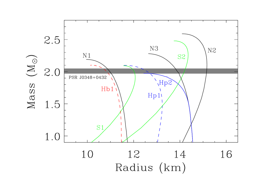
Figure 1: Compact star gravitational mass versus radius curves. Eight curves for non-spinning stars (§ 3) are for eight EoS models (marked by names given in Table 2). The horizontal band shows the mass ($2.01\pm 0.04M_{\odot}$) of the relatively slowly spinning (spin period $=39$ ms) pulsar PSR J0348+0432. This figure shows that all our EoS models can support the mass of this massive pulsar (see § 2).

References

- Abdo et al. (2010) Abdo A. A., Ackermann M., Ajello M., et al. 2010, ApJS, 188, 405
- Akmal et al. (1998) Akmal A., Pandharipande V. R., Ravenhall D. G. 1998, Phys. Rev. C, 58, 1804
- Alford et al. (2005) Alford M., Braby M., Paris M., Reddy S., 2005, ApJ, 629, 969
- Alpar et al. (1982) Alpar M. A., Cheng A. F., Ruderman M. A., Shaham J., 1982, Nature, 300, 728
- Antoniadis et al. (2012) Antoniadis J., van Kerkwijk M. H., Koester D., Freire P. C. C., Wex N., Tauris T. M., Kramer M., Bassa C. G., 2012, MNRAS, 423, 3316
- Antoniadis et al. (2013) Antoniadis J., Freire P. C. C., Wex N., et al., 2013, Science, 340, 448
- Archibald et al. (2009) Archibald A. M., Stairs I. H., Ransom S. M., et al., 2009, Science, 324, 1411
- Backer et al. (1982) Backer D. C., Kulkarni S. R., Heiles C., Davis M. M., Goss W. M., 1982, Nature, 300, 615
- Bagchi (2011) Bagchi M., 2011, MNRAS, 413, L47
- Banik et al. (2014) Banik S., Hempel M., Bandyopadhyay D., 2014, ApJS, 214, 22
- Bardeen (1970) Bardeen J.M., 1970, ApJ, 162, 71
- Barr et al. (2013) Barr E. D., Champion D. J., Kramer M., et al., 2013, MNRAS, 435, 2234
- Bauböck et al. (2013) Bauböck M., Berti E., Psaltis D., Özel F., 2013, ApJ, 777, 68
- Bejger et al. (2011) Bejger M., Zdunik J. L., Haensel P., Fortin M., 2011, A&A, 536, A92
- Bhattacharyya (2002) Bhattacharyya S., 2002, A&A, 383, 524
- Bhattacharyya (2011) Bhattacharyya S., 2011, MNRAS, 415, 3247
- Bhattacharyya et al. (2001a) Bhattacharyya S., Bhattacharya D., Thampan A.V., 2001a, MNRAS, 325, 989
- Bhattacharyya et al. (2016) Bhattacharyya S., Bombaci I., Logoteta D., Thampan A. V., 2016, MNRAS, 457, 3101
- Bhattacharyya et al. (2006) Bhattacharyya S., Miller M. C., Lamb F. K., 2006, ApJ, 644, 1085
- Bhattacharyya et al. (2001b) Bhattacharyya S., Misra R., Thampan A.V., 2001b, ApJ, 550, 841
- Bhattacharyya et al. (2005) Bhattacharyya S., Strohmayer T. E., Miller M. C., Markwardt C. B., 2005, ApJ, 619, 483
- Bhattacharyya et al. (2001c) Bhattacharyya S., Thampan A.V., Bombaci I., 2001c, A&A, 372, 925
- Bhattacharyya et al. (2000) Bhattacharyya S., Thampan A.V., Misra R., Datta B., 2000, ApJ, 542, 473
- Bogdanov et al. (2007) Bogdanov S., Rybicki G. B., Grindlay J. E., 2007, ApJ, 670, 668
- Bogdanov (2013) Bogdanov S., 2013, ApJ, 762, 96
- Bombaci (2007) Bombaci I., 2007, Eur. Phys. J., 31, 810
- Bombaci & Datta (2000) Bombaci I., Datta B., 2000, ApJ, 539, L69
- Bombaci et al. (1995) Bombaci I., Prakash M., Prakash M., Ellis P. J., Lattimer J. M., Brown G. E., 1995, Nucl. Phys. A, 583, C623
- Bombaci et al. (2000) Bombaci I., Thampan A.V., Datta B., 2000, 2000, ApJ, 541, L71
- Burrows & Lattimer (1986) Burrows A., Lattimer J. M. 1986, ApJ, 307, 178
- Chakrabarty & Morgan (1998) Chakrabarty D., Morgan E. H. 1998, Nature, 394, 346
- Champion et al. (2008) Champion D. J., Ransom S. M., Lazarus, P., et al., 2008, AIP Conference Proceedings, 983, 448
- Cipolletta et al. (2015) Cipolletta F., Cherubini C., Filippi S., et al., 2015, Phys. Rev. D, 92, 023007
- Cook et al. (1994) Cook G. B., Shapiro S. L., Teukolsky S. A., 1994, ApJ, 424, 823
- Corongiu et al. (2012) Corongiu A., Burgay M., Possenti A., et al., 2012, ApJ, 760, 100
- D’Amico et al. (2001) D’Amico N., Lyne A. G., Manchester R. N., Possenti A., Camilo F., 2001, ApJ, 548, L171
- Datta et al. (1998) Datta B., Thampan A.V., Bombaci I., 1998, A&A, 334, 943
- de Martino et al. (2013) de Martino D., Belloni T., Falanga M., et al., 2013, A&A, 550, A89
- Demorest et al. (2010) Demorest P., Pennucci T., Ransom S., Roberts M., Hessels J., 2010, Nature, 467, 1081
- Deneva et al. (2013) Deneva J. S., Stovall K., McLaughlin M. A., Bates S. D., Freire P. C. C., Martinez J. G., Jenet F., Bagchi M., 2013, ApJ, 775, 51
- Desvignes et al. (2016) Desvignes G., Caballero R. N., Lentati L., et al. 2016, MNRAS, 458, 3341
- Edwards & Bailes (2001) Edwards R. T., Bailes M., 2001, ApJ, 547, L37
- Fonseca et al. (2016) Fonseca E., Pennucci T. T., Ellis J. A., et al., 2016 (arXiv:1603.00545)
- Foster et al. (1993) Foster R. S., Wolszczan A., Camilo F., 1993, ApJ, 410, L91
- Fraga et al. (2001) Fraga E., Pisarki R.D., Schaffner-Bielich J., 2001, Phys. Rev. D, 63, 121702(R)
- Freire et al. (2011) Freire P. C. C., Bassa C. G., Wex N., 2011, MNRAS, 412, 2763
- Friedman et al. (1986) Friedman J. F., Ipser J. R., Parker L., 1986, ApJ, 304, 115
- Gendre et al. (2003) Gendre B., Barret D., Webb N., A&A, 403, L11, 2003
- Gendreau et al. (2012) Gendreau K. C., Arzoumanian Z., Okajima T., 2012, Proc. SPIE 8443, Space Telescopes and Instrumentation 2012: Ultraviolet to Gamma Ray, 844313
- Ghosh (1995) Ghosh P., 1995, JAA, 16, 289
- Ghosh and Lamb (1978) Ghosh P., Lamb F. K., 1978, ApJ, 223, L83
- Glendenning (1992) Glendenning, N.K 1992, Phys. Rev. D, 46, 1274
- Glendenning (1996) Glendenning, N.K., 1996, Compact Stars: Nuclear Physics, Particle Physics, and General Relativity, Springer Verlag
- Guillemot et al. (2012) Guillemot L., Freire P. C. C., Cognard I., et al., 2012, MNRAS, 422, 1294
- Haensel & Zdunik (1989) Haensel P. Zdunik J. L., 1989, Nature, 340, 617
- Hebeler et al. (2013) Hebeler K., Lattimer J. M., Pethick C. J., Schwenk A., 2013, ApJ, 773, 11
- Hewish et al. (1968) Hewish A., Bell S. J., Pilkington J. D. H., Scott P. F., Collins R. A., 1968, Nature, 217, 709
- Jacoby et al. (2003) Jacoby B. A., Bailes M., van Kerkwijk M. H., Ord S., Hotan A., Kulkarni S. R., Anderson S. B., 2003, ApJ, 599, L99
- Jacoby et al. (2007) Jacoby B. A., Bailes M., Ord S. M., Knight H. S., Hotan A. W., 2007, ApJ, 656, 408
- Johnston et al. (1993) Johnston S., Lorimer D. R., Harrison P. A., et al., 1993, Nature, 361, 613
- Kramer & Wex (2009) Kramer M., Wex N., 2009, Classical and Quantum Gravity, 26, 073001
- Lattimer & Prakash (2001) Lattimer J. M., Prakash M., 2001, ApJ, 550, 426
- Lattimer & Prakash (2005) Lattimer J. M., Prakash M., 2005, Phys. Rev Lett., 94, 111101
- Lattimer & Prakash (2010) Lattimer J. M., Prakash M., 2010, in From Nuclei to Stars, ed. S. Lee, Singapore: WorldScientific, 275
- Lattimer & Schutz (2005) Lattimer J. M., Schutz B. F., 2005, ApJ, 629, 979
- Logoteta et al. (2015) Logoteta D., Vidaña I., Bombaci I., Kievsky A., 2015, Phys. Rev C, 91, 064001
- Lundgren et al. (1993) Lundgren S. C., Zepka A. F., Cordes J. M., 1993, IAU Circ., 5878, 2
- Lynch et al. (2012) Lynch R. S.; Freire P. C. C., Ransom S. M., Jacoby B. A., 2012, ApJ, 745, 109
- Lyne et al. (2004) Lyne A. G., Burgay M., Kramer M., et al., 2004, Science, 303, 1153
- Miller & Lamb (2015) Miller M. C., Lamb F. K., 2015, ApJ, 808, 31
- Nicastro et al. (1995) Nicastro L., Lyne A. G., Lorimer D. R., Harrison P. A., Bailes M., Skidmore B. D., 1995, MNRAS, 273, L68
- Oppenheimer & Volkoff (1939) Oppenheimer J. R., Volkoff G. M., 1939, Physical Review, 55, 374
- Özel & Freire (2016) Özel F., Freire P., 2016, ARAA (arXiv:1603.02698)
- Papitto et al. (2013) Papitto A., Ferrigno C., Bozzo E., et al., 2013, Nature, 501, 517
- Pechenick et al. (1983) Pechenick K. R., Ftaclas C., Cohen J. M., 1983, ApJ, 274, 846
- Prakash et al. (1997) Prakash M., Bombaci I., Prakash M., Ellis P. J., Lattimer J. M., Knorren R., 1997, Phys. Rep. 280, 1
- Providencia & Rabhi (2013) Providência C., Rabhi A., 2013, Phys. Rev. C, 87, 055801
- Pudliner et al. (1995) Pudliner B. S., Pandharipande V. R., Carlson J., Wiringa R. B., 1995, Phys. Rev. Lett., 74, 4396
- Radhakrishnan & Srinivasan (1982) Radhakrishnan V., Srinivasan, G., 1982, Current Science, 51, 1096
- Ransom et al. (2014) Ransom S. M., Stairs I. H., Archibald A. M., et al., 2014, Nature, 505, 520
- Raithel et al. (2016) Raithel C. A.,Özel F., Psaltis D., 2016, arXiv:1605.03591
- Reardon et al. (2016) Reardon D. J., Hobbs G., Coles W., et al., 2016, MNRAS 455, 1751
- Sahu et al. (1993) Sahu P. K., Basu R., Datta B. 1993, ApJ, 416, 267
- Segelstein et al. (1986) Segelstein D. J., Taylor J. H., Rawley L. A., Stinebring D. R., 1986, IAUC, 4162, 2
- Stoks et al. (1993) Stoks V. G. J., Klomp R. A. M., Rentmeester M. C. M., de Swart J. J., 1993, Phys. Rev. C, 48, 792
- Sugahara & Toki (1994) Sugahara Y, Toki H., 1994, Nucl. Phys. A, 579, 557
- Thampan and Datta (1998) Thampan A.V., Datta, B., 1998, MNRAS, 297, 570
- Tolman (1939) Tolman R. C., 1939, Physical Review, 55, 364
- van Paradijs (1978) van Paradijs J., Nature, 274, 650, 1978
- Weissenborn et al. (2011) Weissenborn S., Sagert I., Pagliara G., Hempel M., Schaffner-Bielich J., 2011, ApJ, 740, L14
- Wijnands & van der Klis (1998) Wijnands R., van der Klis M., 1998, Nature, 394, 344
- Wiringa et al. (1995) Wiringa R. B., Stoks V. G. J., Schiavilla R., 1995, Phys. Rev. C, 51, 38