Statistical Mechanics and Hydrodynamics of Self-Propelled Hard Spheres

Abstract

Starting from a microscopic model of self-propelled hard spheres we use tools of non-equilibrium statistical mechanics and the kinetic theory of hard spheres to derive a Smoluchowski equation for interacting Active Brownian particles. We illustrate the utility of the statistical mechanics framework developed with two applications. First, we derive the steady state pressure of the hard sphere active fluid in terms of the microscopic parameters and second, we identify the critical density for the onset of motility-induced phase separation in this system. We show that both these quantities agree well with overdamped simulations of active Brownian particles with excluded volume interactions given by steeply repulsive potentials. The results presented here can be used to incorporate excluded volume effects in diverse models of self-propelled particles.

I Introduction

In recent years, the study of active materials has been on the forefront of research in soft condensed matter physics. A particular class of active materials is one composed of self propelled particles that convert energy from a local bath into persistent motion. Self propelled particles describe systems on many length scales, ranging from bacteria Cates (2012); Berg (2001), synthetic colloids F. et al. (2015); Hong et al. (2007); Palacci et al. (2013), vibrated granular rods Narayan et al. (2007), to schools of fish Marchetti et al. (2013); Ballerini et al. (2008). Despite the fact that there exists continual energy consumption and dissipation at the level of individual particles, collections of self-propelled particles form large-scale, stable, coherent structures Ramaswamy (2010). Phenomena exhibited include athermal phase separation among purely repulsive particles Buttinoni et al. (2013); Cates and Tailleur (2015); Redner et al. (2013); Putzig and Baskaran (2014), anomalous mechanical properties Yang et al. (2014); Takatori et al. (2014); Solon et al. (2015a); Mallory et al. (2014), emergent structures and pattern formation Hagan and Baskaran (2016); Gopinath et al. (2012); Farrell et al. (2012).

Theoretical progress in understanding active materials has been propelled by the study of minimal models for self-propelled particles. The most widely studied of these minimal models is known as an active Brownian particle (ABP). ABPs travel with constant velocity along their body axis and the orientation of their body axis changes through ordinary rotational diffusion. While numerical investigations of ABPs abound in the literature and have led to a significant understanding of the dynamics of this system, analytical progress for interacting particles has been difficult. The reason that analytical descriptions of the collective behavior remain elusive is that interactions have a finite collision time, which in turn would result in intractable many body effects. To overcome this challenge, authors have taken phenomenological approaches such as incorporating the effect of interactions in a density dependence of the self propulsion speed Cates and Tailleur (2015, 2013); Cates (2012); Tailleur and Cates (2009); Solon et al. (2015b) and a mean field version of dynamical density functional theory Bialke et al. (2013); Speck et al. (2014, 2015).

In this paper, we aim to capture these many body effects by applying the well developed theoretical framework of hard-sphere liquids van Beijeren and Ernst (1979); Hansen and McDonald (1990) to a fluid consisting of ABPs. Starting with underdamped Langevin equations to describe the dynamics of self-propelled particles that interact with hard core instantaneous collisions, we systematically coarse grain the microdynamics to obtain a description applicable on longer length and time scales after which we take the limit of large friction to obtain an effective description for an overdamped systems of ABPs. The primary theoretical result in this work is a first principles derivation of the statistical mechanics of self-propelled hard spheres. To illustrate the utility of this result, we compute two well studied emergent properties in fluids of ABPs: the mechanical pressure and the phase boundary that determines the onset of athermal phase separation into a dense liquid and a dilute gas. We then compare our results to those in the literature obtained from numerical studies and more phenomenological theoretical approaches and use this comparison to place the context of our work within the existing body of work.

II Theoretical Framework

II.1 Microdynamics

We consider self propelled hard disks in two dimensions with particle diameter $\sigma$, unit mass, and moment of inertia $I$. The microstate of $N$ such hard disks is given by $\Gamma=\{\mathbf{r}_{1}(t),\dots,\mathbf{r}_{n}(t),\mathbf{v}_{1}(t),\dots,\mathbf{v}_{n}(t),\omega_{1}(t),\dots,\omega_{n}(t),\theta_{1}(t),\dots,\theta_{n}(t)\}$. Here the variables ($\mathbf{r}_{i}$, $\mathbf{v}_{i}$, $\theta_{i}$, $\omega_{i}$) are the position, velocity, orientation, and angular velocity respectively of the $i$ th particle. The equations of motion in this case are given by $\partial_{t}\mathbf{r}_{i}=\mathbf{v}_{i}$ and $\partial_{t}\theta_{i}=\omega_{i}$ where the linear and angular velocities evolve according to

$$\frac{\partial\mathbf{v}_{i}}{\partial t}=\sum_{j\neq i}T(i,j)\mathbf{v}_{i}+F\hat{\mathbf{u}}_{i}-\nabla V(\mathbf{r})-\xi\mathbf{v}_{i}+\bm{\eta}_{i}(t)$$ (1)

$$\frac{\partial\omega_{i}}{\partial t}=-\xi_{R}\omega_{i}+\eta_{i}^{R}(t).$$ (2)

Here, the unit vector $\hat{\mathbf{u}}=(\cos(\theta),\sin(\theta))$ is the orientation of the particle’s body axis along which a propulsive force of strength $F$ acts and $V(\mathbf{r})$ is some external potential. The binary collision operator $T(i,j)$ generates the instantaneous linear momentum transfer between disks at contact and is given by van Beijeren and Ernst (1979)

$$T(i,j)=\sigma\int d\hat{\bm{\sigma}}\Theta(-\mathbf{V}_{ij}\cdot\hat{\bm{\sigma}})|\mathbf{V}_{ij}\cdot\hat{\bm{\sigma}}|\delta(\mathbf{r}_{ij}-\bm{\sigma})(b_{ij}-1)$$ (3)

where $\hat{\bm{\sigma}}$ is the unit normal at the point of contact directed from disk $j$ to disk $i$ and $\mathbf{V}_{ij}=\mathbf{v}_{i}-\mathbf{v}_{j}$. The operator $b_{ij}$ replaces pre-collisional velocities with post-collisional velocities, e.g., $b_{12}\mathbf{v}_{1}=\mathbf{v}_{1}-(\mathbf{V}_{12}\cdot\hat{\bm{\sigma}})\hat{\bm{\sigma}}$   for collisions which conserve energy and momentum. The spatial delta function ensures that particles are in contact. The prefactors that depend on the relative velocities $\mathbf{V}_{ij}$ ensures that the incoming flux of colliding particles is taken into account correctly. The random forces $\bm{\eta}_{i}(t)$ and $\eta_{i}^{R}(t)$ are Gaussian white noise variables with correlations given by $\langle\eta_{i}^{\alpha}(t)\eta_{j}^{\beta}(t^{\prime})\rangle=2k_{B}T\xi\delta_{\alpha\beta}\delta_{ij}\delta(t-t^{\prime})$ and $\langle\eta_{i}^{R}(t)\eta_{j}^{R}(t^{\prime})\rangle=2k_{B}T_{R}\xi_{R}\delta_{ij}\delta(t-t^{\prime})$ respectively. Latin indices label the particle number, while Greek indices label the vector components of the noise. The noise amplitudes depend on parameters $T,T_{R}$ that have the units of temperature. These parameters need not be the same as $T_{R}$ is an intrinsic quantity describing the reorientation of the active drive.

Thus, Eqs.(1-2) are the Langevin equations for $N$ interacting self-propelled hard disks. For a single particle in the high friction limit these equations would reduce to the well studied Redner et al. (2013); Fily and Marchetti (2012); Cates (2012); Romanczuk et al. (2012); Cates and Tailleur (2015); Marchetti et al. (2013); Yang et al. (2014); Takatori et al. (2014); Solon et al. (2015a); Mallory et al. (2014); Farage et al. (2015); Marini Bettolo Marconi and Maggi (2015); Cates and Tailleur (2013); Solon et al. (2015b); Bialke et al. (2013); Tailleur and Cates (2009) overdamped Langevin equations $\partial_{t}\mathbf{r}=v_{0}\hat{\mathbf{u}}+\bar{\bm{\eta}}$ and $\partial_{t}\theta=\bar{\eta}^{R}$ where the self-propulsion velocity is given by $v_{0}=F/\xi$ and the noise terms are given by $\bar{\bm{\eta}}=\bm{\eta}/\xi$ and $\bar{\eta}^{R}=\eta^{R}/\xi_{R}$.

II.2 Statistical Mechanics

Illustration of Coarse-graining Technique: We seek to derive the statistical mechanics of this system of self-propelled hard disks in the large friction limit. One could derive the statistical mechanics from the overdamped Langevin equation mentioned at the end of the previous subsection rather straightforwardly. In this work, we are using hard disks to be able to tractably incorporate the physics of excluded volume interactions into the statistical mechanics. In this case, the large friction limit needs to be taken at the level of the Fokker-Planck equation. In order to illustrate the technique involved, let us begin by considering a collection of noninteracting particles (described by Eqs.(1-2) without the binary collision operator). In this case the statistical mechanics is given by the one particle probability distribution function $f(\mathbf{r},\theta,\mathbf{v},\omega,t)$ of finding a particle with some position $\mathbf{r}$, orientation $\theta$, velocity $\mathbf{v}$, and angular velocity $\omega$ at time $t$. This PDF obeys the Fokker-Planck equation given by Baskaran and Marchetti (2010)

$$\partial_{t}f(\mathbf{r},\theta,\mathbf{v},\omega,t)+\mathcal{D}f(\mathbf{r},\theta,\mathbf{v},\omega,t)=0$$ (4)

and the Fokker-Planck operator $\mathcal{D}$ is given by

$$\mathcal{D}=\mathbf{v}\cdot\nabla_{\mathbf{r}}+\omega\partial_{\theta}+F\hat{\mathbf{u}}\cdot\nabla_{\mathbf{v}}-\nabla_{\mathbf{r}}V(\mathbf{r})\cdot\nabla_{\mathbf{v}}-\xi\nabla_{\mathbf{v}}\cdot\mathbf{v}-\xi_{R}\partial_{\omega}\omega-k_{B}T\xi\nabla_{\mathbf{v}}^{2}-k_{B}T_{R}\xi_{R}\partial_{\omega}^{2}.$$ (5)

Let us define the particle concentration $c(\mathbf{r},\theta,t)=\int d\mathbf{v}d\omega f(\mathbf{r},\theta,\mathbf{v},\omega,t)$, a translational current $\mathbf{J}^{T}=\int d\mathbf{v}d\omega\mathbf{v}f(\mathbf{r},\theta,\mathbf{v},\omega,t)$, and a rotational current $J^{R}=\int d\mathbf{v}d\omega\omega f(\mathbf{r},\theta,\mathbf{v},\omega,t)$. By taking appropriate velocity moments of Eq.(4), one finds that the concentration field obeys a conservation law of the form

$$\partial_{t}c+\nabla_{\mathbf{r}_{1}}\cdot\mathbf{J}^{T}+\partial_{\theta}J^{R}=0.$$ (6)

In the large friction limit, the currents are given by

$$\lim_{t\gg 1/\xi}\mathbf{J}^{T}=-\frac{1}{\xi}\big{[}-F\hat{\mathbf{u}}c+c\nabla V(\mathbf{r})+\nabla\cdot\langle\mathbf{v}\otimes\mathbf{v}\rangle+\partial_{\theta}\langle\omega\mathbf{v}\rangle\big{]}$$ (7a)

$$\lim_{t\gg 1/\xi_{R}}J^{R}=-\frac{1}{\xi_{R}}\big{[}\nabla\cdot\langle\omega\mathbf{v}\rangle+\partial_{\theta}\langle\omega^{2}\rangle\big{]}$$ (7b)

where the brackets in the above represent averages over linear and angular velocities. In order to have a closed equation for the concentration we must evaluate the averages in Eqs.(7a-7b). We assume the PDF can be written as

$$f(\mathbf{r},\theta,\mathbf{v},\omega,t)=\frac{1}{2\pi k_{B}T}\sqrt{\frac{1}{2\pi k_{B}T_{R}}}c(\mathbf{r},\theta,t)e^{-\frac{(\mathbf{v}-v_{0}\hat{\mathbf{u}})^{2}}{2k_{B}T}}e^{-\frac{\omega^{2}}{2k_{B}T_{R}}}$$ (8)

with $v_{0}=F/\xi$. This assumption says that in this large friction regime, there exists separation of time scales for spatial relaxations and velocity relaxations, the latter being fast and so at late times, the velocity distribution has relaxed to its local equilibrium form Baskaran and Marchetti (2010). The velocity averages can then be evaluated and the dynamical equation reads

$$\partial_{t}c+v_{0}\hat{\mathbf{u}}\cdot\nabla c-\xi^{-1}\nabla\cdot\big{[}c\nabla V(\mathbf{r})\big{]}-\nabla\cdot\tensor{\mathbf{D}}\cdot\nabla c-D_{r}\partial_{\theta}^{2}c=0$$ (9)

In the above $D_{r}=\frac{k_{B}T_{R}}{\xi_{r}}$ and the diffusion tensor is of the following form $D_{\alpha\beta}=D_{\parallel}\hat{u}_{\alpha}\hat{u}_{\beta}+D_{\perp}(\delta_{\alpha\beta}-\hat{u}_{\alpha}\hat{u}_{\beta})$. With $D_{\parallel}=v_{0}^{2}\xi^{-1}+k_{B}T\xi^{-1}$ and $D_{\perp}=k_{B}T\xi^{-1}$. Note that in the completely thermal limit we recover ordinary isotropic diffusion $D_{\alpha\beta}=\xi^{-1}k_{B}T\delta_{\alpha\beta}=D_{t}\delta_{\alpha\beta}$. In the purely self-propelled limit we obtain $D_{\alpha\beta}=\xi^{-1}v_{0}^{2}\hat{u}_{1\alpha}\hat{u}_{1\beta}$ as was reported in Baskaran and Marchetti (2010) for self-propelled hard rods. This procedure yields the well studied Smoluchowski equation for ABPs that others have obtained Romanczuk et al. (2012); Solon et al. (2015b); Bialke et al. (2013).

Result: Now, repeating the calculation but retaining the hard core interactions (see Appendix A), the Smoluchowski equation is of the following form

$$\partial_{t}c+\nabla_{\mathbf{r}}\cdot\mathbf{J}^{T}-D_{r}\partial_{\theta}^{2}c=0$$ (10)

Note that the rotational part of the Smoluchowksi equation remains unchanged because no torques are exerted in a collision of smooth disks. However, the translational current has the form

$$\mathbf{J}^{T}=v_{0}\hat{\mathbf{u}}c-\xi^{-1}c\nabla V(\mathbf{r})-\tensor{\mathbf{D}}\cdot\nabla c+\xi^{-1}\big{(}\mathbf{I}^{thermal}+\mathbf{I}^{sp}+\mathbf{I}^{cross}\big{)}.$$ (11)

The first three terms of Eq.(11) are equivalent to the terms in Eq.(9) and the additional terms in Eq.(11) are collisional contributions to the translational current. They are given by

$$I_{\alpha}^{thermal}=\frac{4\pi^{2}\sigma(k_{B}T)^{3}}{(2\pi k_{B}T+v_{0}^{2})^{2}}\int_{\hat{\bm{\sigma}},\theta_{2}}c^{(2)}(\mathbf{r}_{1},\theta_{1},\mathbf{r}_{1}-\bm{\sigma},\theta_{2},t)\hat{\sigma}_{\alpha}$$ (12a)

$$I_{\alpha}^{sp}=\frac{\sigma v_{0}^{6}}{(2\pi k_{B}T+v_{0}^{2})^{2}}\int_{\hat{\bm{\sigma}},\theta_{2}}\Theta(-\hat{\mathbf{u}}_{12}\cdot\hat{\bm{\sigma}})(\hat{\mathbf{u}}_{12}\cdot\hat{\bm{\sigma}})^{2}c^{(2)}(\mathbf{r}_{1},\theta_{1},\mathbf{r}_{1}-\bm{\sigma},\theta_{2},t)\hat{\sigma}_{\alpha}$$ (12b)

$$I_{\alpha}^{cross}=\frac{\sigma}{(2\pi k_{B}T+v_{0}^{2})^{2}}\int_{\hat{\bm{\sigma}},\theta_{2}}c^{(2)}(\mathbf{r}_{1},\theta_{1},\mathbf{r}_{1}-\bm{\sigma},\theta_{2},t)$$ (12c)

$$\times[2\pi(k_{B}T)^{2}v_{0}^{2}+\pi k_{B}Tv_{0}^{4}((\hat{\mathbf{u}}_{1}\cdot\hat{\bm{\sigma}})^{2}+(\hat{\mathbf{u}}_{2}\cdot\hat{\bm{\sigma}})^{2})-\sqrt{8\pi(k_{B}T)^{3}}v_{0}^{3}\hat{\mathbf{u}}_{12}\cdot\hat{\bm{\sigma}}]\hat{\sigma}_{\alpha}$$

and where $\hat{\mathbf{u}}_{12}=\hat{\mathbf{u}}_{1}-\hat{\mathbf{u}}_{2}$.

Discussion:

1. The above collisional contributions in Eq.(10) all have the form of a mean field force, $I_{\alpha}=\int_{\hat{\bm{\sigma}},\theta_{2}}F_{\alpha}(\theta_{1},\theta_{2},\hat{\bm{\sigma}})c^{(2)}(\mathbf{r}_{1},\theta_{1},\mathbf{r}_{1}-\bm{\sigma},\theta_{2},t)$. Where $F_{\alpha}(\theta_{1},\theta_{2},\hat{\bm{\sigma}})$ is some orientation dependent force density and $c^{(2)}(\mathbf{r}_{1},\theta_{1},\mathbf{r}_{1}-\bm{\sigma},\theta_{2},t)$ is the two body probability distribution function of finding particle 1 with position $\mathbf{r}_{1}$ and orientation $\theta_{1}$ and particle 2 with position $\mathbf{r}_{1}-\bm{\sigma}$ and orientation $\theta_{2}$ at a time $t$ (see fig.1).

   

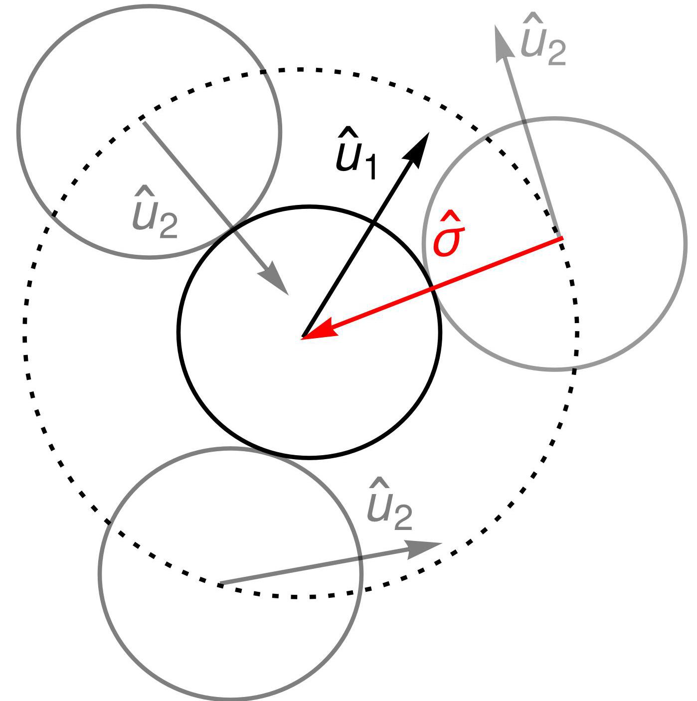
   Figure 1: (color online) An illustration of a collision between particle 1 with orientation $\hat{\mathbf{u}}_{1}(\theta_{1})$ and particle 2 with orientation $\hat{\mathbf{u}}_{2}(\theta_{2})$ . The unit normal vector $\hat{\bm{\sigma}}$ at the point of contact is directed from particle 2 to particle 1. A collision can occur when the center of particle 2 lies anywhere on the dotted line, as illustrated by the gray spheres. The mean field force is obtained by integrating over all configurations $\hat{\mathbf{u}}_{1}$,$\hat{\mathbf{u}}_{2}$ and $\hat{\bm{\sigma}}$

2. In the completely thermal limit ($v_{0}=0$) the only term that would contribute to the collision integral is Eq.(12a) and would reproduce the statistical mechanics of thermal hard spheres in the overdamped limit. This is precisely the contribution one would find starting from the revised Enskog theory Balescu (1975); Lachowicz et al. (1991); Chapman and Cowling (1970).

3. Eq.(12b) is a contribution from collisions arising from self-propulsion alone. Within this equation is a theta function which constrains the range of allowed orientations of the self-propulsion direction of the second particle. That is, the theta function is nonzero only for orientations that would result in a collision.

4. Eq.(12c) is a collisional contribution that arises from the coupling of thermal noise and self-propulsion and contains the leading order contribution to the translational current from the collisions among particles (see Appendix A).

In this section we have outlined the systematic derivation of the statistical mechanics of self-propelled hard spheres. The results described above should be useful to describe any collection of active particles that interact through strongly repulsive short range interactions, as will be shown in later sections. We now illustrate the applicability of the derived statistical mechanics by investigating some macroscopic properties of a fluid of active particles.

III Steady State Mechanical Properties

As a first illustration, we seek to use the statistical mechanics developed above to calculate a steady state property of this system. Let us consider the pressure of an active fluid. As has been shown in Solon et al. (2015a) this is indeed a state variable for self-propelled particles in the absence of any torques as is the case for smooth hard disks considered here. Mechanically one can then define pressure by considering the system as being confined by a wall at some position $x_{w}\gg 0$ (see fig.2).

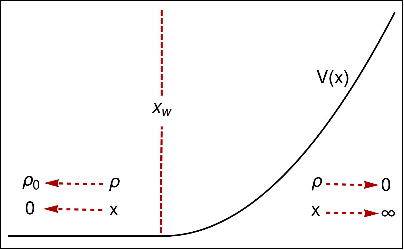
Figure 2: (color online) An illustration of the confining potential

represented by some confining potential $V(x)$ and where $x=0$ is taken to be deep in the bulk of the active particle fluid. We assume that deep in the bulk of the fluid the density has a constant bulk value $\rho_{0}$, far beyond $x_{w}$ the density vanishes, and that the system stays uniform in the $\hat{y}$-direction. By Newton’s 3rd Law, the pressure can be computed from the total force acting on the wall,

$$P=\int_{0}^{\infty}\rho(x)\partial_{x}V(x)dx.$$ (13)

Using the procedure developed in Solon et al. (2015a) (see Appendix B for details), we arrive at the following expression for the pressure

$$P=P_{0}+\int d\theta\bigg{[}\frac{v_{0}}{D_{r}}\hat{u}_{x}(I_{x}^{thermal}+I_{x}^{sp}+I_{x}^{cross})\bigg{|}_{x=0}+\int_{0}^{\infty}(I_{x}^{thermal}+I_{x}^{sp}+I_{x}^{cross})dx\bigg{]}.$$ (14)

In the above, $P_{0}=\big{(}\frac{v_{0}^{2}\xi}{2D_{r}}+\frac{v_{0}^{2}}{2}+k_{B}T\big{)}\rho_{0}$ is the pressure of noninteracting self-propelled particles and $I$’s are the collision kernels given in Eqs. (12a-12c).

To make any further analytic progress we must evaluate integrals over the collisional contributions which involve the two body distribution $c^{\left(2\right)}$. We now make the ansatz that this two body distribution can be written as a functional of the one body distributions in the following way,

$$c^{(2)}(\mathbf{r}_{1},\theta_{1},\mathbf{r}_{2},\theta_{2},t)=g(\mathbf{r}_{1},\mathbf{r}_{2}\big{|}\rho(\mathbf{r},t))c(\mathbf{r}_{1},\theta_{1},t)c(\mathbf{r}_{2},\theta_{2},t),$$ (15)

where $g(\mathbf{r}_{1},\mathbf{r}_{2}\big{|}\rho(\mathbf{r},t))$ is a functional of the density field. For thermal hard spheres, this function $g$ is the equilibrium pair correlation function and it provides an exact functional relationship between the one and two body distributions. In the case of self-propelled particles, this ansatz cannot be exact as we expect orientational correlations to play some role. Such orientational correlations were in fact characterized in Bialke et al. (2013) through the use of density functional theory and simulations. A systematic estimation of $g$, even in the limited form we have chosen is a hard problem that is beyond the scope of the present work. In the following, we use the form of $g$ associated with thermal hard spheres at contact. That is, we assume orientational correlations can be neglected and that positional correlations are accounted for in the same way as for thermal hard spheres. The test of the validity of this assumption will be the comparison to numerical simulations considered later in this presentation. For the rest of the paper we use the well known estimate of the contact pair-correlation function known as the Carnahan-Starling pair-correlation function in 2 dimensions Balescu (1975).

$$g\left(\mathbf{r}_{1},\mathbf{r}_{2}\big{|}\rho(\mathbf{r},t)\right)=g(\sigma|\rho)=\frac{1-\frac{7}{16}\phi}{(1-\phi)^{2}},$$ (16)

where $\phi=\frac{\pi}{4}\rho\sigma^{2}$ is the packing fraction. This estimate is known to give an accurate description of the fluid phase of hard spheres and consequently, this approximation will not capture crystallization effects. We also note that one can choose other estimates of the pair correlation function, such as the Hypernetted Chain Balescu (1975), to approximate density correlations in different parameter regimes. With the ansatz above, the computation of the pressure in Eq.(14) reduces to integrals over the one particle distribution function $c\left(r,\theta\right)$ which is in turn the steady state solution to the Smoluchowski equation Eq.(10). Using the standard procedure Solon et al. (2015b); Baskaran and Marchetti (2008) of representing the distribution as a harmonic expansion in terms of the angular moments, $c=\frac{\rho}{2\pi}+\frac{1}{\pi}\mathbf{P}\cdot\hat{\mathbf{u}}+\tensor{\mathbf{Q}}:(\hat{\mathbf{u}}\hat{\mathbf{u}}-\frac{1}{2}\mathbf{I})+\dots$ where $\mathbf{P}=\int d\theta\hat{\mathbf{u}}c$, is the first moment, $\tensor{\mathbf{Q}}=\int d\theta(\hat{\mathbf{u}}\hat{\mathbf{u}}-\frac{1}{2}\mathbf{I})c$ is the second moment, and assuming a low-moment closure (i.e., truncating the moment expansion at some order, see appendix C for details) we can now evaluate the integrals in Eq.(14) with the result

$$P=P_{0}+\lambda_{D}g(\sigma)\rho_{0}^{2}-g(\sigma)\frac{\xi v_{0}}{D_{r}}\lambda_{I}\rho_{0}^{2}.$$ (17)

In the above, the constants $\lambda_{D}$ and $\lambda_{I}$ control the strength of the collisional contributions to the pressure and depend on the microscopic parameters (see appendix D for the explicit forms). In order to understand the structure of this result, it is useful to consider some limits of Eq.(17). First, in the absence of the self-propulsion (i.e. $v_{0}=0$) we have.

$$P=k_{B}T\rho_{0}\bigg{(}1+\frac{\pi\sigma^{2}g(\sigma)}{2}\rho_{0}\bigg{)}$$ (18)

This is precisely what one would find when calculating the pressure for a hard sphere gas when using Revised-Enskog theory Baskaran et al. (2007); Garzó and Dufty (1999). It consists of the ideal gas term plus an additional correction due to the hard core interactions. In the athermal limit (i.e. $k_{B}T=0$) we obtain

$$P=\frac{v_{0}^{2}}{2D_{r}\xi^{-1}}\rho_{0}+\frac{v_{0}^{2}}{2}\rho_{0}+\frac{3\pi}{16}v_{o}^{2}\sigma^{2}g(\sigma)\rho_{0}^{2}-\frac{2}{3}\frac{v_{0}^{3}\sigma}{D_{r}}g(\sigma)\rho_{0}^{2}$$ (19)

This limit ($k_{B}T=0$) has been simulated in Solon et al. (2015a) using the Weeks-Chandler-Andersen (WCA) potential. Even though this interaction has a finite collision time we find that our expression captures the computed pressure well for low to moderate densities (see fig.3), thus illustrating the validity of our results for systems with short-range strongly repulsive interactions.

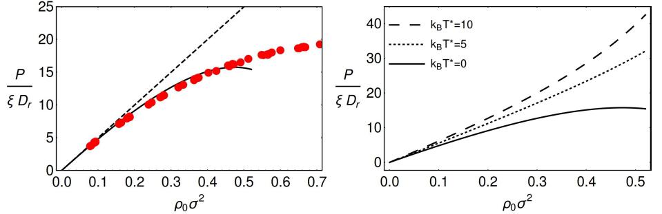
Figure 3: (color online) In this figure Eq.(19) was made dimensionless by $P=P^{\ast}\xi D_{r}$, $v_{0}=v_{0}^{\ast}\sigma D_{r}$, $\rho_{0}=\rho_{0}^{\ast}\sigma^{-2}$, $k_{B}T=k_{B}T^{\ast}\xi\sigma^{2}D_{r}$. Left: The pressure in the athermal limit. The dots are the simulated results of ABPs interacting via the WCA potential. The solid black line is the theoretical expression (Eq.(19)) with a fit parameter $\alpha=D_{r}/\xi=.027$. The dashed line is the noninteracting pressure. Right: The pressure when temperature is included (Eq.(17)) leading to an increase in the pressure as the temperature is increased.

Finally, we compare our result for the pressure with those already in the literature for an overdamped system of ABPs interacting with repulsive potentials. In Solon et al. (2015c), the authors use fluctuating hydrodynamics to derive expressions for the pressure of interacting ABPs in terms of correlation functions between moments of $c(\mathbf{r},\theta,t)$. They find that the pressure can be written as the sum of three terms $P=P_{0}+P_{I}+P_{D}$ where $P_{0}$ is the ideal active pressure and the ”indirect pressure” $P_{I}$ and ”direct pressure” $P_{D}$ are given respectively by $P_{I}=\frac{v_{0}}{D_{r}}\int d^{2}r^{\prime}F_{x}(\mathbf{r}^{\prime})\langle\rho(\mathbf{r}^{\prime})P_{x}(0)\rangle$ and $P_{D}=\int_{0}^{\infty}dx\int d^{2}r^{\prime}F_{x}(\mathbf{r^{\prime}}-\mathbf{r})\langle\rho(\mathbf{r}^{\prime})\rho(\mathbf{r})\rangle$ where $F_{x}$ is the component of the interaction force between particles and the angular brackets here represent an average over the noise. In our theory, we start with a noise averaged dynamical equation. The analogous contributions for the pressure in our case are as follows. The second term in Eq. (14) is the indirect pressure $P_{I}$ and is indeed the evaluation of the corresponding correlation function over the solution of the Smoluchowski equation for the case of hard spheres. The third term in Eq. (14) is the direct pressure $P_{D}$ evaluated for our hard core interactions. We also note that in Solon et al. (2015c) the authors prove that the sum $P_{0}+P_{I}$ is equivalent to the ”swim pressure” investigated by Yang et al. (2014); Takatori et al. (2014) and the same equivalence holds between our theory and the swim pressure as well.

Summarizing, in this section, we have used the statistical mechanics of self propelled hard spheres to tractably evaluate the interaction contributions to the pressure of an active fluid. We have found good agreement with numerical simulations of the pressure of ABPs interacting via a steeply repulsive potential with a finite collision time, thus illustrating the usefulness of the derived statistical mechanics for a variety of model active fluids.

IV Hydrodynamics and Phase Separation

As a second illustration of the utility of the nonequilibrium statistical mechanics constructed here, we derive and characterize a dynamical description of an active fluid on length scales long compared to the particle diameter and time scale long compared to the mean free time. In this regime, the relevant dynamical variables are the conserved quantities and quantities associated with any possible broken symmetries that couple to them. The only conserved quantity is the density of particles given by the zeroth moment of the probability distribution

$$\rho(\mathbf{r},t)=\int d\theta c(\mathbf{r},\theta,t).$$ (20)

The other relevant dynamical quantities are higher angular moments of concentration field. Of these moments, the only relevant quantity that couples to the hydrodynamic field is the polarization described by the first moment of the probability distribution.

$$P_{\alpha}(\mathbf{r},t)=\int d\theta\hat{u}_{\alpha}c(\mathbf{r},\theta,t).$$ (21)

We seek to identify the dynamical equations obeyed by these two quantities.

To derive the continuum equations for the relevant macroscopic fields we must take the corresponding moments of the Smoluchowski equation and they are of the form

$$\partial_{t}\rho=-\nabla\cdot\mathbf{J}$$ (22)

$$\partial_{t}P_{\beta}=-\partial_{\alpha}J_{\alpha\beta}-D_{r}P_{\beta}$$ (23)

where

$$\begin{pmatrix}J_{\alpha}\\ J_{\alpha\beta}\end{pmatrix}=\int d\theta\begin{pmatrix}1\\ \hat{u}_{\beta}\end{pmatrix}J_{\alpha}^{T}.$$ (24)

The fluxes in Eq.(24) are again moments of the two particle distribution as in the case of the pressure calculation above. In order to evaluate these fluxes, we proceed as in the preceding section by assuming the simplest phenomenological closure of the Smoluchowksi equation, that the two particle distribution function can be written as the product of one particle distributions $c^{(2)}(\mathbf{r}_{1},\theta_{1},\mathbf{r}_{1}-\bm{\sigma},\theta_{2},t)=g(\sigma)c^{(1)}(\mathbf{r}_{1},\theta_{1},t)c^{(1)}(\mathbf{r}_{1}-\bm{\sigma},\theta_{2},t)$ and give the one particle distribution function a series representation in terms of its angular moments (Appendix B). As before, we are using the Carnahan-Starling estimate for $g(\sigma)$. Since we are interested in a long wavelength description of the system the nonlocal dependence of the concentration field is expanded in gradients

$$c(\mathbf{r}-\bm{\sigma},\theta_{2},t)=c(\mathbf{r},\theta_{2},t)-\sigma_{\alpha}\partial_{\alpha}c(\mathbf{r},\theta_{2},t)+\dots$$ (25)

Using the above gradient expansion coupled with a low moment closure we arrive the following equations

$$\partial_{t}\rho+v_{0}\nabla\cdot\mathbf{P}-\nabla\cdot[\mathcal{D}(\rho)\nabla\rho]+D_{p}\nabla\nabla:\mathbf{P}\mathbf{P}=0$$ (26)

$$\partial_{t}P_{\gamma}+D_{r}P_{\gamma}+\nabla_{\gamma}\mathcal{P}(\rho)-D_{\perp}\nabla^{2}P_{\gamma}+2\lambda_{I}\big{[}P_{\gamma}(\nabla\cdot\mathbf{P})+(\mathbf{P}\cdot\nabla)P_{\gamma}\big{]}$$ (27)

$$= \nabla\cdot\big{[}\tensor{\mathbf{L}}(P_{\gamma})\nabla\rho\big{]}+\lambda_{2}\big{[}(\nabla\cdot\mathbf{P})\nabla_{\gamma}\rho+(\mathbf{P}\cdot\nabla)\nabla_{\gamma}\rho+\nabla_{\gamma}\left(\mathbf{P}\cdot\nabla\rho\right)\big{]}$$

$$-\nabla\cdot\big{[}K(\rho)\nabla_{\gamma}\mathbf{P}\big{]}-\nabla_{\gamma}\big{[}K(\rho)\nabla\cdot\mathbf{P}\big{]}$$

where the explicit expressions for all the macroscopic parameters and the functions $\mathcal{D}(\rho)$, $K\left(\rho\right)$ and $L_{\alpha\beta}\left(P_{\gamma}\right)$ in terms of the microscopic parameters of the model are given in Appendix D.

These macroscopic equations are complex and nonlinear, with the effect of the repulsive interactions showing up in the coefficients and in the detailed form of the nonlinearities. While careful study of the phase behavior predicted by these equations is warranted, we defer this to future work and make only a few remarks about the structure of these equations. The density equation above has a similar form to those written down for non-interacting ABPs but with a density dependent diffusion coefficient $\mathcal{D}(\rho)$ and a term analogous to the curvature induced flux term found in hydrodynamic theories of orientable active particles Aditi Simha et al. (2003), signifying the fact that the orientation comes with a physical velocity and hence its fluctuations can result in a diffusive flux. The polarization equation does not have a homogeneous nonlinearity reflecting the fact that the interactions among smooth particles are non-aligning, but still has the complex nonlinearities one expects in Toner-Tu type hydrodynamic theories Toner and Tu (1998). Note that $v_{0}\mathbf{P}$ is a measure of the collective self-propulsion velocity of the system and thus encompasses a compressible flow. This is reflected by the presence of the hydrostatic pressure through $\mathcal{P}=\frac{D_{r}}{v_{0}\xi}P$, together with additional Euler order terms $K(\rho)\nabla\cdot\mathbf{P}-\lambda_{2}\mathbf{P}\cdot\nabla\rho$ in the dynamical equation for this flow.

Note that the relaxation of time of Eq.(27) is given by $t=1/D_{R}$. In the rest of this section, we focus on the behavior of this system on times much longer than this characteristic relaxation time. For such times it is reasonable to assume that the polarization has relaxed to its steady state value, i.e., $\partial_{t}\mathbf{P}=0$. Solving for $\mathbf{P}$ in Eq.(27) and substituting into Eq.(26) we find, neglecting higher order gradient terms, the following diffusion equation for the density,

$$\partial_{t}\rho=\nabla\cdot[D_{eff}(\rho)]\nabla\rho],$$ (28)

where the effective density dependent diffusion coefficient is given by

$$D_{eff}(\rho)=\frac{v_{0}^{2}}{2D_{r}}+\mathcal{D}(\rho)-\frac{2v_{0}}{D_{r}}\lambda_{I}\rho.$$ (29)

In the limit $k_{B}T\rightarrow 0$, this effective diffusion coefficient becomes (putting in the explicit forms for $\mathcal{D}(\rho)$ and $\lambda_{I}$ from Appendix D)

$$D_{eff}(\rho)=\frac{v_{0}^{2}}{2D_{r}}+\frac{v_{0}^{2}}{2\xi}+g(\sigma)\frac{3\pi}{8\xi}v_{0}^{2}\sigma^{2}\rho-g(\sigma)\frac{4}{3}\frac{v_{0}^{3}\sigma\rho}{D_{r}\xi}$$ (30)

The last term in Eqs.(29-30) is negative and there exists a critical density $\rho_{c}$ or equivalently a critical packing fraction $\phi_{c}=\rho_{c}\frac{\pi}{4}\sigma^{2}$ above which this diffusion coefficient becomes negative. This signals the onset of clustering in the system that has been referred to in the literature as Motility Induced Phase Separation (MIPS). Using the Carnahan-Starling estimate (Eq.(24)) for $g(\sigma)$ one can identify this critical density as a function of system parameters and this is shown by the black line in fig.4.

To better understand this critical density, it is useful to take some limits. First consider the limit of high Peclet number, in this limit the critical density predicted by Eq.(29) is of the form to $\phi_{c}=\frac{1}{\text{Pe}}\frac{\pi(37+21\alpha)}{224\alpha}$, where $\alpha=\xi/D_{r}$. In the limit $k_{B}T\rightarrow 0$, (i.e., no translational diffusion in the overdamped limit) we obtain the following expression for the critical density,

$$\phi_{c}=-\frac{4\left(-64\alpha+\frac{6\pi(\alpha-2)}{\text{Pe}}+\sqrt{4096\alpha^{2}+\frac{81\pi^{2}\alpha^{2}}{\text{Pe}^{2}}-\frac{243\pi^{2}\alpha}{\text{Pe}^{2}}-\frac{1440\pi\alpha^{2}}{\text{Pe}}+\frac{864\pi\alpha}{\text{Pe}}}\right)}{224\alpha+\frac{\pi(48-15\alpha)}{\text{Pe}}},$$

which again for high enough Peclet number goes as $\phi_{c}\sim\text{Pe}^{-1}$. This $1/\text{Pe}$ behavior has also been seen through phenomenological theories Cates and Tailleur (2015); Marchetti et al. (2016) and in kinetic estimates of the critical density for the onset of MIPS Redner et al. (2013). Finally in fig.4, we compare the estimate provided by this theory against the data from simulations of a system of ABPs interacting through a WCA potential treating $\alpha=\frac{\xi}{D_{r}}$ as a fit parameter and we find good agreement with the data, again illustrating the validity of the result to systems with short range strongly repulsive interactions.

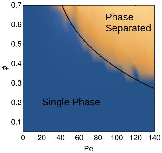
Figure 4: (color online) Numerical results for the phase boundary taken from Redner et al. (2013). Black line is the critical density at which Eq.(29) becomes zero. Here we find good agreement when using $\alpha=.01$ and the dimensionless temperature $k_{B}T^{\ast}=25$. Below the line is the $\mathcal{D}(\rho)>0$ region, above the line is the $\mathcal{D}(\rho)<0$ region.

V Summary & Discussion

In this paper we have provided a derivation of the statistical mechanics for self-propelled hard disks starting from first principles. We then considered two applications of the derived statistical mechanics. First is computing the steady state mechanical pressure of a hard sphere active fluid. In the athermal limit ($k_{B}T=0$) we find good agreement with existing numerical simulations Solon et al. (2015a) of ABPs for low to moderate densities. In the absence of activity ($v_{0}=0$) we reproduce the pressure one finds for thermal hard spheres by using Revised Enskog theory Baskaran et al. (2007). We then derived the hydrodynamic equations describing self-propelled hard spheres and identified the critical density for the onset of MIPS in this system. We find that our prediction fits well the numerical data Redner et al. (2013) from ABP simulations and agrees with earlier phenomenological estimates Redner et al. (2013); Marchetti et al. (2016); Cates and Tailleur (2015) in the large Peclet number regime.

This work uses the theory of hard spheres to circumvent the finite collision time problem and hence many-body effects present in arbitrary repulsive potentials. While an idealization, the results obtained in this paper should be useful for any system of self-propelled particles interacting through strongly repulsive potentials and can be useful for incorporating excluded volume effects into diverse models for active systems. This can be seen in the two applications presented, where we have obtained good agreement with numerical simulations of the overdamped dynamics of ABPs interacting the WCA potential. The statistical mechanics presented here transcends to the two applications we have used to illustrate its utility and is potentially useful in diverse active materials modeling.

Appendix A Derivation of the Smoluchowski equation

We provide a complete derivation of the overdamped dynamics of self-propelled hard disks. Our starting point will be the coupled Langevin equations

$$m\partial_{t}\mathbf{v}_{i}=m\sum_{j\neq i}T(i,j)\mathbf{v}_{i}-\xi\mathbf{v}_{i}+F\hat{\mathbf{u}}_{i}+\bm{\eta}_{i}$$ (31)

$$\partial_{t}\omega_{i}=-\xi_{R}\omega_{i}+\eta_{i}^{R}$$ (32)

where $T(i,j)$ is the binary collision operator given in Eq.(3). The noise function $\bm{\eta}_{i}$ and $\eta_{i}^{R}$ are both Gaussian white noise variables with zero mean and the same correlations defined in the main body of text . The phase space variables associated with the above Langevin dynamics are the position $\mathbf{r}_{n}(t)$, the velocity $\mathbf{v}_{n}(t)$, the angular velocity $\bm{\omega}_{n}(t)$ and the orientation $\theta_{n}(t)$ of the n particles. We begin by considering an arbitrary phase space function $A(\Gamma)$ evaluated at some phase point $\Gamma_{t}=\left\{\mathbf{r}_{1}(t),\dots,\mathbf{r}_{n}(t),\mathbf{v}_{1}(t),\dots,\mathbf{v}_{n}(t),\bm{\omega}_{1}(t),\dots,\bm{\omega}_{n}(t),\theta_{1}(t),\dots,\theta_{n}(t)\right\}$ which has evolved from an initial configuration $\Gamma=\left\{\mathbf{r}_{1},\dots,\mathbf{r}_{n},\mathbf{v}_{1},\dots,\mathbf{v}_{n},\bm{\omega}_{1},\dots,\bm{\omega}_{n},\theta_{1},\dots,\theta_{n}\right\}$. A phase space function at some time t can be expressed in terms of a generator for the dynamics in the following way

$$A(\Gamma_{t})=e^{Lt}A(\Gamma).$$ (33)

In the above equation, $L$ is the sum of generators for translations and rotations for each particle coordinate. For a system with pairwise additive, conservative, non-singular interactions the operator L can be written as

$$L=L_{0}+\frac{1}{2}\sum_{i,j\neq i}m^{-1}\mathbf{F}(r_{ij})\cdot(\nabla_{\mathbf{v}_{i}}-\nabla_{\mathbf{v}_{j}}),$$ (34)

where the single particle component for self propelled particles with a propulsion force $F^{sp}$ along its body axis is given by

$$\begin{split}L_{0}=&\sum_{i}^{N}\{\mathbf{v}_{i}\cdot\nabla_{\mathbf{r}_{i}}+\omega_{i}\partial_{\theta_{i}}+\frac{F^{sp}}{m}\hat{\mathbf{u}}\cdot\nabla_{\mathbf{v}_{i}}-\frac{\xi}{m}\mathbf{v}_{i}\cdot\nabla_{\mathbf{v}_{i}}-\xi_{R}\omega_{i}\partial_{\omega_{i}}\\ &+\frac{1}{m}\bm{\eta}_{i}\cdot\nabla_{\mathbf{v}_{i}}+\eta_{i}^{r}\partial_{\omega_{i}}-\frac{k_{B}T\xi}{m^{2}}\nabla_{\mathbf{v}_{i}}^{2}-\frac{k_{B}T_{R}\xi_{R}}{I}\partial_{\omega_{i}}^{2}\}.\end{split}$$ (35)

The inclusion of the last two terms in the above generator results from using Ito calculus to correctly incorporate the stochastic component of the dynamics. Eq.(35) is the generalization of the completely deterministic case, in which the dynamics are governed by Hamilton’s equations. One can verify that, for Hamiltonian systems, the generator L changes the positions and velocities according to Hamilton’s equations. In this case, L is the linear operator representing the Poisson bracket of its operand with the Hamiltonian for the system Dufty and Baskaran (2005). However, we are considering the stochastic dynamics of elastic hard spheres, thus the interactions must be taking into account via the binary collision operator $T(i,j)$. In this case the operator L becomes

$$L=L_{0}+\frac{1}{2}\sum_{i,j\neq i}T(i,j).$$ (36)

The above formalism completely determines the stochastic dynamics of any observable $A(\Gamma)$ for given initial conditions in phase space. In this study, we would like to write down not the stochastic observable, but its ensemble averaged value for a given ensemble of initial conditions $\hat{\rho}(\Gamma)$. This is represented by the following phase space average

$$\langle A(\Gamma)\rangle_{ens}=\int d\Gamma\hat{\rho}(\Gamma)A(\Gamma,t).$$ (37)

One can equivalently treat the phase space density as the dynamical variable Zwanzig (2001)

$$\langle A(\Gamma)\rangle_{ens}=\int d\Gamma\hat{\rho}(\Gamma,t)A(\Gamma),$$ (38)

and taking the time derivative of both equation yields

$$\int d\Gamma\partial_{t}\hat{\rho}(\Gamma,t)A(\Gamma)=\int d\Gamma\hat{\rho}(\Gamma)\partial_{t}A(\Gamma,t)$$

$$=\int d\Gamma\hat{\rho}(\Gamma)LA(\Gamma,t)$$

$$=-\int d\Gamma\mathcal{L}\hat{\rho}(\Gamma)A(\Gamma,t).$$

Where $\mathcal{L}$ is the adjoint operator to L. The result of this simple manipulation is a Liouville-like equation for the phase space probability density

$$(\partial_{t}+\mathcal{L})\hat{\rho}(\Gamma,t)=0,$$ (39)

with the adjoint operator is given by

$$\begin{split}\mathcal{L}=&\sum_{i}^{N}\{\mathbf{v}_{i}\cdot\nabla_{\mathbf{r}_{i}}+\omega_{i}\partial_{\theta_{i}}+\frac{F^{sp}}{m}\hat{\mathbf{u}}\cdot\nabla_{\mathbf{v}_{i}}-\frac{\xi}{m}\nabla_{\mathbf{v}_{i}}\cdot\mathbf{v}_{i}-\xi_{R}\partial_{\omega_{i}}\omega_{i}\\ &+\frac{1}{m}\bm{\eta}_{i}\cdot\nabla_{\mathbf{v}_{i}}+\eta_{i}^{r}\partial_{\omega_{i}}-\frac{k_{B}T\xi}{m^{2}}\nabla_{\mathbf{v}_{i}}^{2}-\frac{k_{B}T_{R}\xi_{R}}{I}\partial_{\omega_{i}}^{2}\}-\frac{1}{2}\sum_{i,j\neq i}\bar{T}(i,j).\end{split}$$ (40)

In Eq.(40), the single particle component has been identified by an integration by parts, while the collision operator $\bar{T}(i,j)$ has been explicitly constructed using the restituting collisions Baskaran and Marchetti (2010)

$$\bar{T}(i,j)=\sigma\int d\hat{\bm{\sigma}}\Theta(\mathbf{V}_{ij}\cdot\hat{\bm{\sigma}})(\mathbf{V}_{ij}\cdot\hat{\bm{\sigma}})[b_{ij}^{-1}\delta(\mathbf{r}_{ij}-\bm{\sigma})-\delta(\mathbf{r}_{ij}+\bm{\sigma})].$$ (41)

In the above, $b_{ij}^{-1}$ is the generator of restituting collisions $(b_{ij}^{-1}A(x_{i}^{\prime},x_{j}^{\prime})=A(x_{i},x_{j}))$ which replaces post collisional velocities with its pre-collisional values. Finally, we average over the noise $\rho=\langle\hat{\rho}\rangle$. The resulting equation is given by

$$(\partial_{t}+\mathcal{L})\rho(\Gamma,t)=0,$$ (42)

with the operator $\mathcal{L}$ given by

$$\begin{split}\mathcal{L}=&\sum_{i}^{N}\{\mathbf{v}_{i}\cdot\nabla_{\mathbf{r}_{i}}+\omega_{i}\partial_{\theta_{i}}+\frac{F^{sp}}{m}\hat{\mathbf{u}}\cdot\nabla_{\mathbf{v}_{i}}-\frac{\xi}{m}\nabla_{\mathbf{v}_{i}}\cdot\mathbf{v}_{i}-\xi_{R}\partial_{\omega_{i}}\omega_{i}\\ &-\frac{k_{B}T\xi}{m^{2}}\nabla_{\mathbf{v}_{i}}^{2}-\frac{k_{B}T_{R}\xi_{R}}{I}\partial_{\omega_{i}}^{2}\}-\frac{1}{2}\sum_{i,j\neq i}\bar{T}(i,j).\end{split}$$ (43)

The above equation governs the time evolution of the phase space density of N self-propelled hard spheres. To proceed, we now introduce reduced distribution functions

$$f^{(n)}(\Gamma_{1},\dots,\Gamma_{n},t)=\frac{N!}{(N-n)!}\int d\Gamma_{n+1}\dots d\Gamma_{N}\rho(\Gamma_{1}\dots,\Gamma_{N},t)$$ (44)

and consider the first equation of the resulting hierarchy

$$\partial_{t}f^{(1)}(\Gamma_{1},t)+\mathcal{D}f^{(1)}(\Gamma_{1},t)=\int d\Gamma_{2}\bar{T}(1,2)f^{(2)}(\Gamma_{1},\Gamma_{2},t).$$ (45)

Where the one particle operator $\mathcal{D}$ in Eq.(45) is given by

$$\mathcal{D}=\mathbf{v}_{i}\cdot\nabla_{\mathbf{r}_{i}}+\bm{\omega}_{i}\cdot\partial_{\theta_{i}}+\frac{F^{sp}}{m}\hat{\mathbf{u}}\cdot\nabla_{\mathbf{v}_{i}}-\frac{\xi}{m}\nabla_{\mathbf{v}_{i}}\cdot\mathbf{v}_{i}-\xi_{R}\partial_{\omega_{i}}\omega_{i}-\frac{k_{B}T\xi}{m^{2}}\nabla_{\mathbf{v}_{i}}^{2}-\frac{k_{B}T_{R}\xi_{R}}{I}\partial_{\omega_{i}}^{2}.$$ (46)

The goal of this section is to obtain a dynamical equation for the local concentration field by

$$c^{(1)}(\mathbf{r}_{1},\theta_{1},t)=\int d\mathbf{v}_{1}f^{(1)}(\mathbf{r}_{1},\mathbf{v}_{1},\theta_{1},\bm{\omega}_{1},t).$$ (47)

For convenience, we introduce a translational and rotational current defined as the velocity moments of the 1-particle distribution function

$$\mathbf{J}^{T}=\int d\omega_{1}d\mathbf{v}_{1}\mathbf{v}_{1}f^{(1)}(\mathbf{r}_{1},\mathbf{v}_{1},\theta_{1},\bm{\omega}_{1},t)$$ (48)

$$J^{R}=\int d\omega_{1}d\mathbf{v}_{1}\omega_{1}f^{(1)}(\mathbf{r}_{1},\mathbf{v}_{1},\theta_{1},\bm{\omega}_{1},t).$$ (49)

Taking velocity moments of Eq.(45), we arrive at the following equations

$$\partial_{t}c^{(1)}+\nabla_{\mathbf{r}_{1}}\cdot\mathbf{J}^{T}+\partial_{\theta_{1}}J^{R}=0$$ (50)

$$\partial_{t}J_{\alpha}^{T}+\frac{\xi}{m}J_{\alpha}^{T}-\frac{F^{sp}}{m}\hat{u}_{1\alpha}c^{(1)}+\partial_{\mathbf{r}_{1}\beta}\langle v_{1\alpha}v_{1\beta}\rangle+\partial_{\theta_{1}}\langle\omega_{1}v_{1\alpha}\rangle=I_{\alpha}^{T}$$ (51)

$$\partial_{t}J^{R}+\xi_{R}J^{R}+\partial_{\mathbf{r}_{1}\beta}\langle\omega_{1}v_{1\beta}\rangle+\partial_{\theta_{1}}\langle\omega_{1}^{2}\rangle=I^{R}.$$ (52)

In the above,

$$\langle v_{1\alpha}v_{1\beta}\rangle=\int d\omega_{1}d\mathbf{v}_{1}v_{1\alpha}v_{1\beta}f^{(1)}(\mathbf{r}_{1},\mathbf{v}_{1},\theta_{1},\bm{\omega}_{1},t)$$ (53)

$$\langle\omega_{1}v_{1\alpha}\rangle=\int d\omega_{1}d\mathbf{v}_{1}\omega_{1}v_{1\alpha}f^{(1)}(\mathbf{r}_{1},\mathbf{v}_{1},\theta_{1},\bm{\omega}_{1},t)$$ (54)

$$\langle\omega_{1}^{2}\rangle=\int d\omega_{1}d\mathbf{v}_{1}\omega_{1}^{2}f^{(1)}(\mathbf{r}_{1},\mathbf{v}_{1},\theta_{1},\bm{\omega}_{1},t),$$ (55)

are the second velocity moments of the probability distribution function. Also present are the following terms

$$I_{\alpha}^{T}=\int d\Gamma_{2}\int d\omega_{1}d\mathbf{v}_{1}v_{1\alpha}\bar{T}(1,2)f^{(2)}(\Gamma_{1},\Gamma_{2},t)$$ (56)

$$I^{R}=\int d\Gamma_{2}\int d\omega_{1}d\mathbf{v}_{1}\omega_{1}\bar{T}(1,2)f^{(2)}(\Gamma_{1},\Gamma_{2},t)=0.$$ (57)

Eq.(56) arises from the linear momentum transfer due to collisions. The integral in Eq.(57) equates to zero because these are smooth hard discs and therefore, no angular momentum is transferred in a collision. The translational and rotational currents in the above equations are subject to frictional damping and as such relax on time scales of order $m/\xi$. On time scales $t\gg m/\xi$ the flux can be approximated as

$$\lim_{t\gg m/\xi}J_{\alpha}^{T}=-\frac{m}{\xi}\big{[}-\frac{F^{sp}}{m}\hat{u}_{1\alpha}+\partial_{\mathbf{r}_{1}\beta}\langle v_{1\alpha}v_{1\beta}\rangle+\partial_{\theta_{1}}\langle\omega_{1}v_{1\alpha}\rangle-I_{\alpha}^{T}\big{]}$$ (58)

$$\lim_{t\gg 1/\xi_{R}}J_{=}^{R}-\frac{1}{\xi_{R}}\big{[}\partial_{\mathbf{r}_{1}\beta}\langle\omega_{1}v_{1\beta}\rangle+\partial_{\theta_{1}}\langle\omega_{1}^{2}\rangle\big{]}$$ (59)

Velocity Integration

To complete the derivation of the Smoluchowski equation, we must evaluate the velocity integrals in Eqs.(58-59). As outlined in section II of the main text, we assume that on these timescales the velocity distributions have relaxed to their local equilibrium form. Explicitly we have that

$$f(\mathbf{v})f(\omega)=Ne^{\frac{-m}{2k_{B}T}(\mathbf{v}-v_{0}\hat{\mathbf{u}})^{2}}e^{-\frac{I\omega^{2}}{2k_{B}T_{R}}},$$ (60)

where N is a normalization factor. With this distribution, it is readily shown that

$$\langle\omega_{1}v_{1\alpha}\rangle=\langle\omega_{1}v_{1\beta}\rangle=0$$ (61)

$$\langle\omega_{1}^{2}\rangle=\frac{k_{B}T}{I}$$ (62)

$$\langle v_{\alpha}v_{\beta}\rangle=(v_{0}^{2}+\frac{k_{B}T}{m})\hat{u}_{\alpha}\hat{u}_{\beta}+\frac{k_{B}T}{m}(\delta_{\alpha\beta}-\hat{u}_{\alpha}\hat{u}_{\beta}).$$ (63)

The above averages are exact for the one-body terms, but for the collision integral (which depends on the orientation of the colliding particles and an integration over the two body distribution), the exact evaluation of the velocity integrals is not possible. To continue further, we make the following asymptotic approximation that accurately captures the physics in the limits that $v_{0}^{2}\gg k_{B}T/m$ (or $k_{B}T/m\gg v_{0}^{2}$)

$$f(v)=\frac{1}{2\pi k_{B}Tm^{-1}+v_{0}^{2}}(e^{-\frac{mv^{2}}{2k_{B}T}}+v_{0}^{2}\delta(\mathbf{v}-v_{0}\hat{\mathbf{u}})).$$ (64)

The delta function enforces that the particle will have a self-propulsion velocity $v_{0}$ along its body axis $\hat{\mathbf{u}}$ and reproduces the the correct distribution in the athermal limit. The Maxwellian accounts for thermal noise and reproduces the statistical mechanics of thermal hard spheres in the limit of zero self-propulsion.

The last step is to perform the velocity averaging in Eq.(56). Explicitly we must evaluate the following,

$$\int d\mathbf{v}_{1}d\mathbf{v}_{2}v_{1\alpha}\bar{T}(1,2)f(\mathbf{v}_{1})f(\mathbf{v}_{2}).$$ (65)

This evaluation of this integral leads to Eqs.(12a-12c) for $I^{thermal}_{\alpha}$, $I^{active}_{\alpha}$, and $I^{cross}_{\alpha}$. To evaluate $I^{cross}_{\alpha}$, which comes from the cross terms in the multiplication of the velocity distributions, one must make an additional approximation. Contained within the integral for the cross terms, one finds terms like

$$\int d\mathbf{v}_{1}\Theta(\mathbf{v}_{1}\cdot\hat{\bm{\sigma}}-v_{0}\hat{\mathbf{u}}_{2}\cdot\hat{\bm{\sigma}}).$$ (66)

Since the integral is over all possible velocities, to good approximation we have

$$\int d\mathbf{v}_{1}\Theta(\mathbf{v}_{1}\cdot\hat{\bm{\sigma}}-v_{0}\hat{\mathbf{u}}_{2}\cdot\hat{\bm{\sigma}})\approx\int d\mathbf{v}_{1}\Theta(\mathbf{v}_{1}\cdot\hat{\bm{\sigma}}).$$ (67)

Using this approximation, the integrals can be computed. The integrals leading to $I^{thermal}_{\alpha}$ and $I^{active}_{\alpha}$ can be computed exactly. These are the most important contributions since, in the limits of purely self-propelled or purely thermal, these are the only contributing factors. This completes the derivation of the Smoluchowski equation. Combining Eq.(50), Eqs.(58-59) and the velocity averages yields Eqs.(10-11) in the main text.

Appendix B Derivation of Pressure

To evaluate this expression we start with the Smoluchowski equation (Eq.(10)). In steady state, the Smoluchowksi equation takes the following form

$$\nabla\cdot\big{[}v_{0}\hat{\mathbf{u}}c-\xi^{-1}\nabla V(\mathbf{r})c-\tensor{\mathbf{D}}\cdot\nabla c+\xi^{-1}\big{(}\mathbf{I}^{thermal}+\mathbf{I}^{sp}+\mathbf{I}^{cross}\big{)}\big{]}+D_{r}\partial_{\theta}^{2}c=0.$$ (68)

Because of the translational invariance in $\hat{y}$, in steady state, the only spatial dependence in the above is through the x-coordinate. Integrating Eq.(68) over the orientations $\theta$, on can see clearly that the resulting equation is of the form $\partial_{x}J^{T}=0$ with $J^{T}$ being the particle current. Since this system has impermeable boundary conditions ($J^{T}=0$ at the wall), the only admissible solution is that $J^{T}=0$ everywhere. Written explicitly we have,

$$\int d\theta c\partial_{x}V=\xi\int d\theta\big{[}v_{0}\hat{u}_{x}c-D_{xx}\partial_{x}c+\xi^{-1}(I^{thermal}_{x}+I^{sp}_{x}+{I}^{cross}_{x})\big{]}.$$ (69)

Rewriting the left hand side of Eq.(69) in terms of the density by noting that $\rho=\int cd\theta$ and by integrating over x, we obtain the pressure (Eq.(13)) written in terms of the concentration field

$$P=\int_{0}^{\infty}dx\int d\theta\xi[v_{0}\hat{u}_{x}c-D_{xx}\partial_{x}c+\xi^{-1}(I^{thermal}_{x}+I^{sp}_{x}+I^{cross}_{x})].$$ (70)

Now let us multiply Eq.(68) by $\hat{u}_{x}$ and integrate over $\theta$

$$D_{r}\int d\theta\hat{u}_{x}c=-\partial_{x}\int d\theta\big{[}\hat{u}_{x}\hat{u}_{x}v_{0}c-\xi^{-1}\hat{u}_{x}c\partial_{x}V-\hat{u}_{x}D_{xx}\partial_{x}c+\xi^{-1}\hat{u}_{x}(I^{thermal}_{x}+I^{sp}_{x}+I^{cross}_{x})\big{]},$$ (71)

and now integrate Eq.(71) over x. Note that the right hand side of Eq.(71) is given as a total derivative and therefore trivially integrated. Aside from the interaction terms in Eq.(71), the only surviving term is the angular integral over $\hat{u}_{x}\hat{u}_{x}c$ which is proportional $\rho/2$. The remaining terms vanish because there can be no orientational order in the bulk of the fluid $(x=0)$ or at $x=\infty$. With these facts, we have that

$$D_{r}\int_{0}^{\infty}dx\int d\theta\hat{u}_{x}c=\frac{v_{0}}{2}\rho_{0}+\int d\theta\xi^{-1}\hat{u}_{x}(I^{thermal}_{x}+I^{sp}_{x}+I^{cross}_{x})\bigg{|}_{x=0}.$$ (72)

Using Eq.(72) to eliminate the first term on the right hand side of Eq.(70) we recover Eq.(14)

$$P=P_{0}+\int d\theta\bigg{[}\frac{v_{0}}{D_{r}}\hat{u}_{x}(I^{thermal}_{x}+I^{sp}_{x}+I^{cross}_{x})\bigg{|}_{x=0}+\int_{0}^{\infty}(I^{thermal}_{x}+I^{sp}_{x}+I^{cross}_{x})dx\bigg{]}.$$ (73)

Appendix C Evaluation of Mean-Field Force and Low Moments Closure

In this section we give the explicit evaluation of the mean-field force (Eqs.(12a-12c)) and an outline of the low moment closure procedure used in the text. To construct the low moment closure we first represent the concentration field as the following harmonic expansion Ahmadi et al. (2006)

$$c(\mathbf{r},\theta,t)=\sum_{m=0}^{\infty}a^{m}_{i_{1}\dots i_{m}}(\mathbf{r},t)T^{m}_{i_{1}\dots i_{m}}(\theta),$$ (74)

where the irreducible tensors $T^{m}_{i_{1}\dots i_{m}}(\theta)$ are equivalent to the spherical harmonics but expressed here in Cartesian coordinates. For illustrative purposes, the first four irreducible tensors are given by

$$T^{0}=1$$ (75)

$$T^{1}_{i}=\hat{u}_{i}$$ (76)

$$T^{2}_{ij}=\hat{u}_{i}\hat{u}_{j}-\frac{1}{2}\delta_{ij}$$ (77)

$$T^{3}_{ijk}=\hat{u}_{i}\hat{u}_{j}\hat{u}_{k}-\frac{1}{4}(\delta_{ij}\hat{u}_{k}+\delta_{ik}\hat{u}_{j}+\delta_{jk}\hat{u}_{i}).$$ (78)

The $m$ th order moment $a^{m}_{i_{1}\dots i_{m}}(\mathbf{r},t)$ of the concentration is given by

$$a^{m}_{i_{1}\dots i_{m}}(\mathbf{r},t)=\frac{1}{2\pi}\int d\theta T^{m}_{i_{1}\dots i_{m}}(\theta)c(\mathbf{r},\theta,t).$$ (79)

The dynamical equation for the $m$ th moment can then be obtained by taking moments of the Smoluchowksi equation (Eq.(10)), with the result

$$\partial_{t}a^{m}_{i_{1}\dots i_{m}}(\mathbf{r},t)=-m^{2}D_{r}a^{m}_{i_{1}\dots i_{m}}(\mathbf{r},t)-\partial_{\alpha}\int d\theta T^{m}_{i_{1}\dots i_{m}}(\theta)J^{T}_{\alpha}.$$ (80)

We see that when written in this form, the density and polarization are just given as the zeroth and first moment of the concentration field. The low moment closure is the approximation that $c(\mathbf{r}_{1},\theta_{1},t)$ can be expressed as a functional of the first two moments $c^{(1)}(\theta_{1};\{\rho(\mathbf{r},t),P_{\alpha}(\mathbf{r},t)\})$. The motivation for this closure is the following: One can see from Eq.(80) that all moments greater than the zeroth moment have a finite relaxation rate given by $m^{2}Dr$. Thus, these moments will relax to values that depend on gradients of the local concentration. When the values of the higher moments are substituted into the density equation they result in terms that are irrelevant compared to the terms resulting from the polarization equation, i.e., contain more powers of gradients and fields. Therefore, we close the expansion by assuming that the second and higher moments can be neglected. This implies that $\int d\theta\hat{u}_{i}\hat{u}_{j}c=\frac{1}{2}\delta_{ij}\rho$ and $\int d\theta\hat{u}_{i}\hat{u}_{j}\hat{u}_{k}c=\frac{1}{4}(\delta_{ij}P_{k}+\delta_{ik}P_{j}+\delta_{jk}P_{i})$. We note that this is a valid closure in the absence of aligning interactions because the density and polarization represent the relevant macroscopic fields. To accurately capture the effects of aligning interactions one must include the second moment as is done in Farrell et al. (2012); Baskaran and Marchetti (2008); Hancock and Baskaran (2015). With this we can now evaluate the mean field force. The mean field force consists of three parts $I_{\alpha}^{thermal}$, $I_{\alpha}^{sp}$, and $I_{\alpha}^{cross}$. To evaluate these quantities we first make the functional ansatz used in the main body of the text, namely that $c^{(2)}(\mathbf{r}_{1},\theta_{1},\mathbf{r}_{1}-\bm{\sigma},\theta_{2},t)=g(\sigma)c(\mathbf{r}_{1},\theta_{1},t)c(\mathbf{r}_{1}-\bm{\sigma},\theta_{2},t)$. We then gradient expand the nonlocal dependence of the concentration field $c(\mathbf{r}-\bm{\sigma},\theta_{2},t)=c(\mathbf{r},\theta_{2},t)-\sigma_{\alpha}\partial_{\alpha}c(\mathbf{r},\theta_{2},t)+\dots$ , which is valid in a long wavelength (hydrodynamic) description of the system. To first order in gradients the integrals can be evaluated. The result of this integration is

$$I_{\alpha}^{thermal}=-\frac{\sigma^{2}4\pi^{2}(k_{B}T)^{3}}{(2\pi k_{B}T+v_{0}^{2})^{2}}g(\sigma)\partial_{\alpha}\rho(\mathbf{r},t)c(\mathbf{r}_{1},\theta_{1},t)$$ (81)

$$I_{\alpha}^{sp}=g(\sigma)\frac{\sigma v_{0}^{6}}{(2\pi k_{B}T+v_{0}^{2})^{2}}\bigg{[}-\frac{4}{3}\hat{u}_{1\alpha}\rho+\frac{4}{3}P_{\alpha}-\frac{\pi\sigma}{4}\big{(}\hat{u}_{1\alpha}\hat{u}_{1\beta}\partial_{\beta}\rho+\hat{u}_{1\beta}\partial_{\beta}P_{\alpha}+\hat{u}_{1\alpha}\partial_{\beta}P_{\beta}-\partial_{\alpha}\rho\big{)}\bigg{]}c(\mathbf{r}_{1},\theta_{1},t)$$ (82)

$$I_{\alpha}^{cross}=g(\sigma)\frac{\sigma k_{B}T}{(2\pi k_{B}T+v_{0}^{2})^{2}}\bigg{[}2\pi(k_{B}T)^{1/2}v_{0}^{3}\big{(}P_{\alpha}-\hat{u}_{1\alpha}\rho\big{)}-\sigma\big{(}2\pi^{2}k_{B}Tv_{0}^{2}+\frac{8+\pi}{4}\pi v_{0}^{4}\big{)}\partial_{\alpha}\rho$$ (83)

$$+\frac{\sigma\pi^{2}}{2}v_{0}^{4}\hat{u}_{1\alpha}\hat{u}_{1\beta}\partial_{\beta}\rho\bigg{]}c(\mathbf{r}_{1},\theta_{1},t).$$

Appendix D Constants and functions used in the hydrodynamics and pressure

For convenience, let us call $A=(2\pi k_{B}T+v_{0}^{2})^{-1}$ and $a=(1+\frac{v_{0}^{2}}{2k_{B}T})$. The constants in the hydrodynamic equations and pressure are then given by

$$D_{p}=\frac{1}{\xi}\frac{\pi}{4}g(\sigma)\sigma^{2}A^{2}v_{0}^{6}$$ (84)

$$\lambda_{I}=\frac{1}{2\xi}A^{2}\sigma g(\sigma)[\frac{4}{3}v_{0}^{6}+v_{0}^{3}(2\pi k_{B}T)^{3/2}]$$ (85)

$$\lambda_{D}=\xi(\mathcal{D}(\rho_{0})-\frac{D_{\parallel}}{2}-D_{\perp}\big{)}$$ (86)

$$\lambda_{2}=\frac{D_{p}}{4}+\frac{1}{3}v_{0}^{4}\sigma^{2}A^{2}\pi\frac{k_{B}T}{\xi}g(\sigma)$$ (87)

and the functions are given by

$$K(\rho)=\frac{1}{2}D_{p}\rho$$ (88)

$$L_{\alpha\beta}(P_{\gamma})=\frac{A^{2}k_{B}Tg(\sigma)\sigma^{2}}{\xi}P_{\gamma}\delta_{\alpha\beta}\bigg{[}a(2\pi k_{B}T)^{2}+(\frac{3\pi^{2}}{8}+2)v_{0}^{4}+\frac{(2+3\pi)\pi-16}{4\pi}\frac{v_{0}^{6}\pi}{k_{B}T}\bigg{]}$$ (89)

$$\mathcal{D}(\rho)=\big{(}\frac{D_{\parallel}}{2}+D_{\perp}\big{)}+\bigg{(}a(2\pi k_{B}T)^{2}+\frac{3}{8}\frac{v_{0}^{6}\pi}{k_{B}T}+\frac{\pi+4}{2}v_{0}^{4}\bigg{)}\frac{A^{2}k_{B}Tg(\sigma)\sigma^{2}}{\xi}\rho$$ (90)

References

- Cates (2012) M. E. Cates, Rep. Prog. Phys. 75, 042601 (2012).
- Berg (2001) H. E. Berg, E. Coli in Motion, Springer (2001).
- F. et al. (2015) G. F., I. Theurkauff, D. Levis, C. Ybert, L. Bocquet, L. Berthier, and C. Cottin-Bizzone, Phys. Rev. X 5, 011004 (2015).
- Hong et al. (2007) Y. Hong, N. M. K. Blackman, N. D. Kopp, A. Sen, and D. Velegol, Phys. Rev. Lett. 99, 178103 (2007).
- Palacci et al. (2013) J. Palacci, S. Sacanna, A. P. Steinberg, D. J. Pine, and P. M. Chaikin, Science 339, 936 (2013).
- Narayan et al. (2007) V. Narayan, S. Ramaswamy, and N. Menon, Science 317, 105 (2007).
- Marchetti et al. (2013) M. C. Marchetti, J. F. Joanny, S. Ramaswamy, T. B. Liverpool, J. Prost, M. Rao, and R. A. Simha, Rev. Mod. Phys. 85, 1143 (2013).
- Ballerini et al. (2008) M. Ballerini, N. Cabibbo, R. Candelier, A. Cavagna, E. Cisbani, I. Giardina, V. Lecomte, A. Orlandi, G. Parisi, A. Procaccini, M. Viale, and V. Zdravkovic, PNAS 105, 1232 (2008).
- Ramaswamy (2010) S. Ramaswamy, Ann. Rev. Cond. Mat. Phys. 1, 323 (2010).
- Buttinoni et al. (2013) I. Buttinoni, J. Bialke, F. Kümmel, H. Löwen, C. Bechinger, and T. Speck, Phys. Rev. Lett. 110, 238301 (2013).
- Cates and Tailleur (2015) M. E. Cates and J. Tailleur, Ann. Rev. Cond. Matt. Phys. 6, 219 (2015).
- Redner et al. (2013) G. S. Redner, M. F. Hagan, and A. Baskaran, Phys. Rev. Lett. 110, 055701 (2013).
- Putzig and Baskaran (2014) E. Putzig and A. Baskaran, Phys. Rev. E. 90, 042304 (2014).
- Yang et al. (2014) X. Yang, M. L. Manning, and M. C. Marchetti, Soft Matter 10, 6477 (2014).
- Takatori et al. (2014) S. C. Takatori, W. Yan, and J. F. Brady, Phys. Rev. Lett 113, 028103 (2014).
- Solon et al. (2015a) A. P. Solon, Y. Fily, A. Baskaran, M. E. Cates, Y. Kafri, M. Kardar, and J. Tailleur, Nat. Phys. 11, 673 (2015a).
- Mallory et al. (2014) S. A. Mallory, A. Šarić, C. Valeriani, and A. Cacciuto, Phys. Rev. E 89, 052303 (2014).
- Hagan and Baskaran (2016) M. F. Hagan and A. Baskaran, Current Opinion in Cell Biology (2016).
- Gopinath et al. (2012) A. Gopinath, M. F. Hagan, M. C. Marchetti, and A. Baskaran, Phys. Rev. E 85, 061903 (2012).
- Farrell et al. (2012) F. D. C. Farrell, M. C. Marchetti, D. Marenduzzo, and J. Tailleur, Phys. Rev. Lett. 108, 248101 (2012).
- Cates and Tailleur (2013) M. E. Cates and J. Tailleur, EPL 101, 20010 (2013).
- Tailleur and Cates (2009) J. Tailleur and M. Cates, EPL 86, 60002 (2009).
- Solon et al. (2015b) A. P. Solon, M. E. Cates, and J. Tailleur, EPJ ST 224, 1231 (2015b).
- Bialke et al. (2013) J. Bialke, H. Lowen, and T. Speck, EPL 103, 3 (2013).
- Speck et al. (2014) T. Speck, J. Bialké, A. M. Menzel, and H. Löwen, Phys. Rev. Lett. 112, 218304 (2014).
- Speck et al. (2015) T. Speck, A. M. Menzel, J. Bialké, and H. Löwen, J. Chem. Phys. 142, 224109 (2015).
- van Beijeren and Ernst (1979) H. van Beijeren and M. Ernst, Journal Stat. Phys. 21, 2 (1979).
- Hansen and McDonald (1990) J. Hansen and I. McDonald, Theory of Simple Liquids, Academic Press, USA (1990).
- Fily and Marchetti (2012) Y. Fily and M. C. Marchetti, Phys. Rev. Lett. 108, 235702 (2012).
- Romanczuk et al. (2012) P. Romanczuk, M. Bär, W. Ebeling, B. Lindner, and L. Schimansky-Geier, EPJ ST 202, 1 (2012).
- Farage et al. (2015) T. F. F. Farage, P. Krinninger, and J. M. Brader, Phys. Rev. E. 91, 042310 (2015).
- Marini Bettolo Marconi and Maggi (2015) U. Marini Bettolo Marconi and C. Maggi, Soft Matter 11, 8768 (2015).
- Baskaran and Marchetti (2010) A. Baskaran and M. C. Marchetti, J. Stat. Mech. 2010, P04019 (2010).
- Balescu (1975) R. Balescu, Equilibrium and Nonequilibrium Statistical Mechanics, John Wiley and Sons, New York (1975).
- Lachowicz et al. (1991) M. Lachowicz, N. Bellomo, and J. Polewczak, Mathematical Topics in Nonllinear Kinetic Theory II: The Enskog Equation, World Scientific Publishing, USA (1991).
- Chapman and Cowling (1970) S. Chapman and T. Cowling, Mathematical Theory of Non-uniform Gases, Cambridge University Press, Cambridge (1970).
- Baskaran and Marchetti (2008) A. Baskaran and M. C. Marchetti, Phys. Rev. E 77, 011920 (2008).
- Baskaran et al. (2007) A. Baskaran, J. W. Dufty, and J. J. Brey, J. Stat. Mech. 2007, P12002 (2007).
- Garzó and Dufty (1999) V. Garzó and J. W. Dufty, Phys. Rev. E 59, 5895 (1999).
- Solon et al. (2015c) A. P. Solon, J. Stenhammar, R. Wittkowski, M. Kardar, Y. Kafri, M. E. Cates, and J. Tailleur, Phys. Rev. Lett. 114, 198301 (2015c).
- Aditi Simha et al. (2003) R. Aditi Simha, S. Ramaswamy, and J. Toner, EPL 62, 196 (2003).
- Toner and Tu (1998) J. Toner and Y. Tu, Phys. Rev. E 58, 4828 (1998).
- Marchetti et al. (2016) M. C. Marchetti, Y. Fily, S. Henkes, A. Patch, and D. Yllanes, Current Opinion in Colloid and Interface Science (2016).
- Dufty and Baskaran (2005) J. W. Dufty and A. Baskaran, Nonlinear Dynamics in Astronomy and Physics, S. Gottesman ed., Annals of the New York Academy of Sciences 1045 (2005).
- Zwanzig (2001) R. Zwanzig, Nonequilibrium Statistical Mechanics, Oxford University Press, USA (2001).
- Ahmadi et al. (2006) A. Ahmadi, M. C. Marchetti, and T. B. Liverpool, Phys. Rev. E 74, 061913 (2006).
- Hancock and Baskaran (2015) B. Hancock and A. Baskaran, Phys. Rev. E 92, 052143 (2015).