Plasmid segregation and accumulation

Abstract

The segregation of plasmids in a bacterial population is investigated. Hereby, a dynamical model is formulated in terms of a size-structured population using a hyperbolic partial differential equation incorporating non-local terms (the fragmentation equation). For a large class of parameter functions this PDE can be re-written as an infinite system of ordinary differential equations for the moments of its solution. We investigate the influence of different plasmid production modes, kinetic parameters, and plasmid segregation modes on the equilibrium plasmid distribution. In particular, at small plasmid numbers the distribution is strongly influenced by the production mode, while the kinetic parameters (cell growth rate resp. basic plasmid reproduction rate) influence the distribution mainly at large plasmid numbers. The plasmid transmission characteristics only gradually influence the distribution, but may become of importance for biologically relevant cases. We compare the theoretical findings with experimental results.

1 Introduction

Plasmids are self-replicating, extra-chromosomal DNA molecules most commonly found in bacteria. Genes coded on naturally occurring plasmids typically support the survival under various environmental conditions such as antibiotic resistance, specific degradation pathways, virulence, amongst others. In genetics and biotechnology plasmids serve as important tool to express particular genes e.g. for the recombinant production of proteins [30]. In low-copy plasmids the copy number ranges from 1-2 copies per cell. During cell division those plasmids are actively segregated like chromosomes via a so called partitioning system. The copy number of high-copy plasmids can be up to several hundred molecules per cell. Although it is questioned, the general assumption is, that high-copy plasmids without partitioning system segregate stochastically by random diffusion [19].

The dynamics of the plasmid distribution in a bacterial population is of interest, e.g., in order to understand the spread of new properties, but also in order to optimize processes in biotechnological engineering. In particular, recent experimental findings show an accumulation of high copy plasmids in some cells [22]. To understand the background of this accumulation is of large interest, as for biotechnological production techniques, neither cells with only few plasmids nor cells with too many plasmids are desired: cells with only few plasmids do not produce efficiently as they are insufficiently triggered to do so, and cells with too many plasmids will not produce well as the metabolic costs for plasmid reproduction are too high.

Modeling plasmid distributions has a rather long tradition. Most approaches are based on simulation models of a population structured by the number of plasmids per cell [1, 16, 10, 23]. Only few articles go to a continuum limit, and consider a hyperbolic partial differential equation [9]. All these models indicate that an unimodal distribution should be expected, resembling a gamma distribution. These papers do not address plasmid accumulation, but rather the condition of plasmid loss.

Experimental findings show that high copy plasmids are in general not equally distributed among the daughter cells, but often one of the daughters receives systematically a higher fraction of plasmids than the other daughter [22]. The implication of the characteristics of such an unequal transition from mother to daughter is unclear and under discussion [14]. Summers and Sheratt conjecture that this unequal transition also influences the plasmid distribution in a crucial way [27]. One hypothesis states that this characteristics is a key mechanism that leads to aggregation of many plasmids in some cells.

In order to address this hypothesis, we propose a simple model that focuses on the basic mechanisms. We do not consider horizontal transmission of plasmids (neither directly from cell to cell by competent cells, nor by de novo infection due to environmental plasmids), but only vertical spread from mothers to daughters. We also do not assume that the plasmid load affects the population dynamics of bacteria. We focus in particular on the interplay between plasmid and bacterial reproduction, taking into account the characteristics of plasmid segregation. We treat plasmids as an infectious disease that is exclusively spread by vertical transmission, that is, the infectivity is taken to zero. In contrast to epidemic models (and plasmids can be considered as infectious agents), in our model plasmid spread and cell reproduction are strongly intertwined, which leads to difficulties in separating information about population and plasmid dynamics. We obtain a hyperbolic partial differential equation, the so-called fragmentation equation, with a structure close cell size models [5, 12, 31, 32], see also the book of Perthame [24] and quotations therein. A lot of work is done for cell size models, in particular the asymptotic behaviour is well known. We give some overview about the most important existence results in section 3. In the present paper, the primarily aim is not to extend results about existence and asymptotic stability of an equilibrium distribution, but aim at a characterization of its asymptotic shape.
In order to disentangle plasmid and cell population dynamics, we focus on moments. The zero’th moment corresponds to the population size, the first moment to the amount of plasmids within the population etc. We find an infinite systems of ordinary differential equations for these moments.
At this point, we introduce two fundamentally different production mechanisms for plasmid production: In the plasmid-controlled mode (also called mass-controlled mode [16]) each plasmid reproduces itself, such that the reproduction rate is in lowest order proportional to the plasmid number. In the cell controlled mode, basically the cell determines the plasmid production rate, such that the rate is to a large extend independent on the number of plasmids present. For the plasmid controlled mode, we obtain a fundamental threshold theorem: the population loses plasmids if cell reproduction is faster than plasmid reproduction. Threshold theorems of this type are well known from the theory of communicable diseases. In the cell controlled mode, plasmids are of course never lost. Next we concentrate on the equilibrium distribution of plasmids in the population. In particular we aim to identify reasons that lead to aggregation of plasmids in cells. It turns out that aggregation of plasmids is first of all influenced by the ratio between basic plasmid reproduction rate and cell reproduction rate. If this factor is less than two, we find that the distribution tends to zero at the carrying capacity of plasmids. If this factor exceeds two, a singularity builds up at the carrying capacity: the distribution tends to infinity, indicating aggregation of many plasmids in some cells. The characteristics of plasmid segregation does influence this shape, but is only of minor importance.

The paper is structured as follows: in section 2 we introduce the discrete model and the continuum limes that yields the hyperbolic partial differential equation and discuss in section 3 some relevant literature and state some simple properties of the equation. In section 4 we reformulate the PDE in terms of moments, and analyze the shape of plasmid distribution in several scenarios for the plasmid reproduction. We deepen this discussion of the influence of parameters on the plasmid distribution in section 5, basically by means of numerical simulations. Section 6 compares theoretical and experimental results, and in the last section 7 we discuss our findings.

2 Model

2.1 Discrete Model

We start with a model discrete in state, similarly to [1]. The population size of bacteria containing $i$ plasmids at time $t$ is denoted by $x_{i}(t)$ (see also table 1 for the meaning of the parameters). The processes that mainly affect the dynamics of $x_{i}$ are cell division (and cell death) that decrease the number of plasmids per cell, and plasmid reproduction that increases the plasmid number per cell. Cell- and plasmid reproduction counteract and their interplay determines the plasmid distribution (see figure 1). The reproduction rate of plasmids within a cell already containing $i$ plasmids is $\tilde{b}(i)$. Later, we will specify $\tilde{b}(i)$ such that different scenarios can be analyzed.

Figure 1: Mechanisms implemented in the model: plasmids reproduce within cells, cells divide, and during cell division plasmids are transferred from mother to daughters.

Cells die at rate $\mu$, and reproduce at rate $\beta$. We assume that neither the death- nor the division rate is affected by the number of plasmids contained by a cell. At this point, it would be simple (and more realistic) to include a plasmid-dependence of these rates. However, as we restrict ourselves exclusively to constant rates in the present work, we stay with this basic case.
Next the transmission of plasmids from mother to daughter is modeled. Very often, bacteria are shaped like small cylinders. One side of the cylinder (bottom or top) is tagged - this is the pole of the cell. One of the daughter cells inherits the old pole of the mother cell. In this way, the two daughter cells can be distinguished. If the mother contained $i$ plasmids, we denote by $p(j;i)$ the probability that the daughter inheriting the mother’s pole obtains $j$ plasmids (consequently, the other daughter receives $i-j$ plasmids). The average number of daughters containing $j$ plasmids in case that the mother contains $i$ plasmids is given by $p(j;i)+p(i-j;i)$. We will identify different transmission characteristics and investigate their effect. Since we do not distinguish between the daughter cell incorporating the mothers pole and that incorporating a new pole, even an unequal segregation leads to a symmetric shape of $p(j;i)+p(i-j;i)$. Unequal segregation is likely to produce a bimodal shape, while equal segregation will in most biologically relevant cases result in an unimodal shape.
Cells divide at rate $\beta$, and in this, leave their population class $x_{i}$. This process yields a term $-\beta x_{i}$ in the model. The daughter cells are distributed to population classes with less or equal many plasmids. Equivalently, all daughters that receive $i$ plasmids enter $x_{i}$. Their mothers necessarily contained $i$ or more plasmids. These model assumptions lead to a description of the cell division (and only cell division) by the equation

$$x_{i}^{\prime}=-\beta x_{i}+\beta\sum_{i^{\prime}=i}^{\infty}[p(i;i^{\prime})+p(i^{\prime}-i;i^{\prime})]x_{i^{\prime}}.$$

We formally extend the sum to infinity, though in biologically relevant situations we expect a maximal number of plasmids a cell will contain, such that eventually $x_{i}=0$. Note that

$$\sum_{i=0}^{i^{\prime}}[p(i;i^{\prime})+p(i^{\prime}-i;i^{\prime})]=2$$ (1)

and

$$\sum_{i=0}^{i^{\prime}}i\,[p(i;i^{\prime})+p(i^{\prime}-i;i^{\prime})]=\sum_{i=0}^{i^{\prime}}i\,p(i;i^{\prime})-\sum_{i=0}^{i^{\prime}}(i^{\prime}-i)p(i^{\prime}-i;i^{\prime})+\sum_{i=0}^{i^{\prime}}i^{\prime}\,p(i;i^{\prime})\\ =i^{\prime}.$$

These two equations indicate that the number of cells is doubled and the number of plasmids is conserved in cell divisions.
All in all, we obtain for $x_{i}$ the system of ordinary differential equations

$$x_{i}^{\prime} = -(\beta+\mu)x_{i}+\tilde{b}(i-1)\,x_{i-1}-\tilde{b}(i)\,x_{i}$$

$$\qquad\qquad\qquad\qquad+\beta\sum_{i^{\prime}=i}^{\infty}[p(i;i^{\prime})+p(i^{\prime}-i;i^{\prime})]x_{i^{\prime}}$$

where we formally take $x_{-1}(t)\equiv 0$. As the experiments we will consider below are performed for high copy plasmids (that is, $x_{i}\not=0$ for $i$ large), we proceed towards the continuum limit. Since also the cell population is large, stochastic effects can be assumed to be negligible.

	discrete model	continuous model
Amount of plasmids	$i$	$z$
Population size at time $t$	$x_{i}(t)$	$u(z,t)$
Cell division rate	$\beta$	$\beta$
Cell death rate	$\mu$	$\mu$
Plasmid reproduction rate	$\tilde{b}(i)$	$b(z)$
Plasmid transmission kernel	$p(i;i^{\prime})+p(i^{\prime}-i;i^{\prime})$	$k(x,y)$

Table 1: Parameters for the discrete and the continuous model.

2.2 Continuum limit

In order to proceed to the continuum limit, we assume at the time being that there is a smooth function $u(z,t)$ such that for $h$ small

$$x_{i}(t)\approx\int_{i\,h-h/2}^{i\,h+h/2}u(z,t)\,dz\approx u(i\,h,t)\,h,$$

and that $\tilde{b}(i)\approx b(h\,i)/h$, $p(i;i^{\prime})+p(i^{\prime}-i;i^{\prime})\approx h\,k(i\,h,i^{\prime}\,h)$. Eqn. (1) indicates that

$$\int_{0}^{y}k(x,y)\,dx=2$$ (3)

and its definition implies a certain symmetry,

$$k(y-x,y)=k(x,y).$$

In the limit $h\rightarrow 0$, we obtain

$$\partial_{t}u(z,t)+\partial_{z}(b(z)u(z,t)) = -(\beta+\mu)u(z,t)+\beta\int_{z}^{\infty}k(z,z^{\prime})u(z^{\prime},t)\,dz^{\prime}$$ (4)

with $u(z,t)\in L^{1}$ for $t$ given. The plasmid reproduction rate $b(z)$ is the flux of this hyperbolic partial differential equation. We superimpose zero flux boundary conditions at $z=0$,

$$b(0)u(0,t)=0.$$ (5)

If $b(0)=0$, this condition is trivial, but we also intend to consider the rather extreme case that $b(z)\equiv b_{0}$ is constant. If $b(z)$ posses a strictly positive limit for $z\rightarrow 0+$, this boundary condition is required. We obtain the fragmentation equation as stated e.g. in the book of Perthame [24].

Remark 2.1

The structure of the model is unexpectedly different from most epidemic models, where the dynamics of the endemics is formulated as the fate of one subpopulation, the class of infected individuals. Here, instead, the dynamics (and the parameters) of the infection are hidden in the flux of the size structure. Epidemic models close to the present approach address e.g. explicitly the parasite load per individual [13]. Nevertheless, there is still a fundamental difference in spreading parasites and plasmids: An individual can transmit parasites horizontally to other individuals, while in our restricted model plasmids can be only passed from mother to daughter (vertical transmission). Standard epidemic models incorporate some aspect of irreducibility missing in the present context. In that aspect, a model that allows for plasmid release and uptake may be even more simple to handle than the present one.
One central issue below will be to separate and compare information about the population dynamics of bacteria and population dynamics of plasmids.

3 Existence results, simple properties

Fragmentation-aggregation processes did attract attention, particularly in recent years. We briefly indicate known results, particularly existence results; the main focus of the present paper is not existence results but properties of the long term behavior.

The fragmentation-aggregation equation we obtained has a structure close to cell size models [5, 12, 31, 32], see also the book of Perthame [24] and quotations therein. A lot of work is done for cell size models, in particular the asymptotic behavior is well known. In cell size models, a singularity appears if cells reach a critical size, as the rate at which cells divide tends to infinity at this size. This is a singularity in the reaction term of the equation. In the present case, the singularity appears in the plasmid dynamics within cells. That is, the flow of the hyperbolic equation becomes singular (i.e., the flow becomes zero). As stated in [7], often there is no biological justification to assume a non-singular flow in the transport equation, but only few articles address this problem, see e.g. [18, 6, 7, 20, 4].
As the model is linear, we expect in non-pathological cases that the solution approximates in the long run an exponentially growing solution. It is central to study the eigenvalue problem

$$\partial_{z}(b(z)U(z)) = -(\beta+\mu+\lambda)U(z)+\beta\int_{z}^{\infty}k(z,z^{\prime})U(z^{\prime})\,dz^{\prime}$$

$$b(0)U(0) = 0,\qquad\lambda\in\mathbb{R},\qquad U\geq 0,\quad U(z)\not\equiv 0.$$

Often, in addition it is assumed that $U$ is at least continuous; this condition rules out solutions that have a point mass at zero, and therefore it is often possible to obtain uniqueness results (even if $b(0)=0$). Convergence of the initial value problem towards $e^{\lambda t}\,c\,U(z)$ for $c\in\mathbb{R}$ suited are available in the case that $k(x,y)=2\,\delta(x-y/2)$, $b=1$, $\mu=0$, and $\beta$ is continuous [25], and can often be concluded by the “general relative entropy method” (see [24] for more general $k$).
Particularly, existence and convergence results are known in case that $b(z)$ is constant [24], $b(z)=z^{\alpha}$ [18, 3], or $b(z)$ has compact support (under the assumption that $\beta(0)=0$) [6]. In [7], more general parameter functions $b(z)$ are allowed, but e.g. $\beta(z)/b(z)$ needs to be integrable at $z=0$. To our knowledge, the existence of the solution $U(z)$ in case of logistic growth $b(z)=b_{0}z(1-z/z_{0})$ and $\beta$ constant is not exactly handled. As mentioned before, we also do not address the existence problem, but give an illustrative example for special parameters, where $U(z)$ can be explicitly determined.

In view of the biological question we aim to answer, we focus on properties of $U(z)$. Before we start with this investigation, we note some obvious properties of the model. As usual, we denote by $\mathbb{R}_{+}=\{x\geq 0\}$, $\|\varphi\|_{C^{1}(\mathbb{R}_{+})}=\sup_{x\in\mathbb{R}_{+}}(|\varphi(x)|+|\varphi^{\prime}(x)|)$, and $L^{1}(\mathbb{R}_{+})$ is the space of Lebesgue-integrable functions on $\mathbb{R}_{+}$. The first lemma indicates that an initial value with a compact support will always have a compact support.

Lemma 3.1

(a) Assume $b(z)=b_{0}z(1-z/z_{0})$ or $b(z)=b_{0}(1-z/z_{0})$, $z_{0}>0$. Let $u_{0}(z)\in L^{1}(\mathbb{R}_{+})$, ${\rm supp}(u_{0})\subset[0,z_{0}-\varepsilon]$. Then, for all $t\in\mathbb{R}_{0}$ there is a smooth, monotonously decreasing function $\varepsilon(t)>0$ such that ${\rm supp}(u(z,t))\subset[0,z_{0}-\varepsilon(t)]$.
(b) Assume $b(z)>0$ for $z>0$, and $\|b(z)\|_{C^{1}(\mathbb{R}_{+})}<\infty$. Let $u_{0}(z)\in L^{1}$, where ${\rm supp}(u_{0})$ is a compact interval. Then, for all $t\in\mathbb{R}_{0}$ ${\rm supp}(u_{0})$ stays compact.

Proof: ad a. First of all, if $b(z_{0})=0$ for some $z_{0}>0$ (first zero), then the position of the characteristic lines of the partial differential equation at hand indicates that ${\rm supp}(u(z,t)))\subset[0,z_{0}]$ for any initial condition with support in $[0,z_{0}]$. Since we assume that $b(z)$ is differentiable, we even know that the support of any solution bounded away from $z_{0}$ may get arbitrary close but stays away from $z_{0}$ (in finite time).
ad b. Since $\|b(z)\|_{C^{1}(\mathbb{R})}<\infty$, the solution of the characteristic equations cannot blow up in finite time, and the support of $u(z,t)$ stays finite. ∎

The simplicity of the population growth yields the following result.

Problem 3.2

Let the assumption of lemma 3.2 be given. Then,

$$\int_{0}^{\infty}u(z,t)\,dz=e^{(\beta-\mu)t}\int_{0}^{\infty}u(z,0)\,dz.$$

Proof: Integrating equation (4) from zero to infinity is equivalent with integrating over a finite interval, since the support of $u(z,t)$ for $t$ finite, given, is contained in a (growing, but for all times compact) interval. We find

$$\frac{d}{dt}\int_{0}^{\infty}u(z,t)\,dz = -b(z)u(z,t)\big{|}_{z=0}^{\infty}-(\beta+\mu)\int_{0}^{\infty}u(z,t)\,dz$$

$$\qquad+\beta\int_{0}^{\infty}\int_{z}^{\infty}k(z,z^{\prime})u(z^{\prime})\,dz^{\prime}\,dz$$

With $b(z)u(z,t)\big{|}_{z=0}^{\infty}=0-b(0)u(0,t)=0$ and

$$\int_{0}^{\infty}\int_{z}^{\infty}k(z,z^{\prime})u(z^{\prime})\,dz^{\prime}\,dz=\int_{0}^{\infty}\int_{0}^{z^{\prime}}k(z,z^{\prime})u(z^{\prime})\,dz\,dz^{\prime}=2\int_{0}^{\infty}u(z,t)\,dz$$

we obtain

$$\frac{d}{dt}\int_{0}^{\infty}u(z,t)\,dz = (\beta-\mu)\int_{0}^{\infty}u(z,t)\,dz$$

and the result follows.∎

Note that in general it is non-trivial to determine the exponential growth rate $\lambda$ (see e.g. [24]). The simplicity of our model assumptions yield the following proposition.

Corollary 3.3

Any solution of the form $u(z,t)=U(z)\,e^{\lambda t}$ with $U\in L^{1}(0,z_{0})$ necessarily has exponent $\lambda=\beta-\mu$.

4 Shape of the equilibrium plasmid distribution

We aim at the answer of two questions. (a) Are plasmids able to spread in the population, or does the average number of plasmids per cell tends to zero? (b) If plasmids stay abundant, how does the stationary distribution of plasmids look like? Respectively, can we identify factors that lead to an accumulation of plasmids in some cells?

We will disentangle the dynamics of plasmids and cell population up to a certain degree in addressing not directly the solution $u(z,t)$ respectively the function $U(z)$, but in focusing on the moments $M_{i}(t)=\int_{0}^{\infty}z^{i}\,u(z,t)\,dz$ respectively $P_{i}=\int_{0}^{\infty}z^{i}\,U(z)\,dz$. $M_{0}(t)$ indicates the total population size (regardless how many plasmids are present), $M_{1}(t)$ states the amount of plasmids contained by the total population (summarized over all cells), and $M_{2}(t)$ gives a hint about the variation of the plasmid distribution etc. In this way, the different aspects (population dynamics of bacteria resp. plasmids) can be – up to a certain degree – considered separately.

In order to reduce the partial differential equation for $u(z,t)$ to an infinite set of ordinary differential equations for $M_{i}(t)$, we first investigate moments of the kernel $k(x,y)$ (see also [24, Section 4.2] or [20, Section 1.2] for the next results).

Lemma 4.1

Assume $k(x,y)=k(y-x,y)$, and $\int_{0}^{y}k(x,y)\,dx=2$ for $y>0$. Then, $\int_{0}^{y}x\,k(x,y)\,dx=y$.

Proof: We find

$$\int_{0}^{y}x\,k(x,y)\,dx=\int_{0}^{y}(y-x)\,k(y-x,y)\,dx=\int_{0}^{y}(y-x)\,k(x,y)\,dx=2y-\int_{0}^{y}x\,k(x,y)\,dx.$$

Thus, $\int_{0}^{y}x\,k(x,y)\,dx=y$.∎

Definition 4.2

Let $k(x,y)\geq 0$, $\int_{0}^{y}|k(x,y)|\,dx<\infty$ for $y>0$. If the moments of $k(x,y)$ satisfy

$$\int_{0}^{y}x^{i}k(x,y)\,dx=y^{i}\alpha_{i}$$ (6)

with $\alpha_{i}=\int_{0}^{1}\xi^{i}k(\xi,1)\,d\xi$, $\alpha_{0}=2$, $\alpha_{1}=1$, $\alpha_{i}>\alpha_{i-1}$, and $\sum_{i=1}^{\infty}\alpha_{i}/i<\infty$ for $i\rightarrow\infty$, we call the kernel scalable.

Note that it is straightforward to formulate this definition not only for integrable kernels but also for kernels consisting of distributions (e.g. $\delta$-peaks). The condition $\sum_{i=1}^{\infty}\alpha_{i}/i<\infty$ forces $\alpha_{i}$ to converge sufficiently fast to zero; we will use this fact later in the paper. The next lemma explains why we call kernels characterized by definition 4.2 “scalable”. In particular, we find that the condition $\sum_{i=1}^{\infty}\alpha_{i}/i<\infty$ corresponds to a certain integrability condition for $k(x,y)$.

Lemma 4.3

Let $k(x,y)>0$, and $\int_{0}^{y}\ln(1/(1-x))\,k(x,y)\,dx<\infty$ for $y\in[0,1]$. If $\int_{0}^{y}k(x,y)\,dx=2$, $k(x,y)=k(y-x,y)$, and

$$k(x,y)=k(x/y,1)/y,$$

the kernel $k(x,y)$ is scalable.

Proof: Assume that $\int_{0}^{y}k(x,y)\,dx=1$, $k(x,y)=k(y-x,y)$, and $k(x,y)=k(x/y,1)/y$. Then,

$$\int_{0}^{y}x^{i}k(x,y)\,dx=\int_{0}^{y}x^{i}k(x/y,1)/y\,dx=y^{i}\int_{0}^{1}\xi^{i}k(\xi,1)\,d\xi.$$

We already know that $\alpha_{0}=2$ and $\alpha_{1}=1$ (equation (3) resp. lemma 4.1). The monotonicity of $\alpha_{i}$ and the fact that the sequence tends to zero follows from $\alpha_{i}=\int_{0}^{1}\xi^{i}k(\xi,1)\,d\xi$. Moreover,

$$\infty>\int_{0}^{1}\ln(1/(1-x))\,|k(x,1)|\,dx=\int_{0}^{1}\sum_{i=1}^{\infty}\frac{x^{i}}{i}k(x,1)\,dx=\sum_{i=1}^{\infty}\alpha_{i}/i.$$

∎

In difference to non-scalable kernels, scalable kernels distribute plasmids in a similar way to the daughter cells, independently on the amount of plasmids the mother cell contains. In the case of low copy plasmids, there are plasmid-distribution systems ensuring that all daughter cells receive at least one plasmid. If we have very few plasmids, the distribution law for plasmids may explicitly depend on the number of available plasmids in a non-scalable way. However, if there are more than only few plasmids present, we expect a scalable law to appear. In particular, as we consider the continuum limit for high copy plasmids, the assumption of scalable kernels seems to be reasonable.
We again indicate that the kernel $k(x,y)$ always inherits the symmetry $k(y,x)=k(x-y,x)$ as we do not distinguish between the two daughters. Unequal segregation can be recognized in biological sensible cases by bimodal, equal segregation by unimodal shapes of the kernel.

Example 4.4

$k(x,y)=2\,\delta(x-y/2)$, with

$$\alpha_{i}=\int_{0}^{1}x^{i}k(x,1)\,dx=2^{1-i}.$$

In this case, necessarily both daughter cells obtain the same number of plasmids. Plasmid segregation is necessarily symmetric.

Example 4.5

$k(x,y)=(2/y)\,\chi_{[0,y]}(x)$, with

$$\alpha_{i}=\int_{0}^{1}x^{i}k(x,1)\,dx=\frac{2}{i+1}.$$

Example 4.6

Now we give an example for an asymmetric plasmid distribution between the daughters. One daughter receives more plasmids, to be precise, $(1+a)y/2$ plasmids. Then, the other daughter cell receives $(1-a)y/2$ plasmids. This setup is modeled by the kernel $k(x,y)=\delta(x-(1-a)y/2)+\delta(x-(1+a)y/2)$, with $0\leq a<1$ and

$$\alpha_{i}=\int_{0}^{1}x^{i}k(x,1)\,dx=2^{-i}\left\{(1-a)^{i}+(1+a)^{i}\right\}.$$

Note that the kernel $k(x,y)$ still possesses a symmetric shape, though the underlying plasmid distribution mechanism is unsymmetrical. It is clear that there is also a symmetric plasmid segregation mechanism that yields the very same kernel.

From these examples we conclude that an unequal segregation mechanism is likely to increase the variance in the kernel. This observation allows to reformulate our initial problem: The question is, if a kernel with a high variance leads to accumulation of plasmids in a subpopulation, or if the variance has only a minor effect on the plasmid distribution.

Remark 4.7

Prescribe a sequence $(a_{i})_{i\in{\mathbb{N}}_{0}}$. The task to find a measure $\nu(x)$ with support $[0,1]$ such that $a_{i}=\int_{0}^{1}x^{i}\,d\nu(x)$ is called Hausdorff moment problem. Necessary and sufficient conditions are known that guarantee a solution for the problem. Moreover, if a solution exists, it is unique [28]. However, the moment problem is ill posed, such that naive numerical algorithms to reconstruct the measure from the moments are bound to fail. For us it is sufficient to note that the moments $\alpha_{i}$ defined above provide the complete information about a given, scalable kernel $k(x,y)$; in principle, it is possible to reconstruct $k(x,y)$ from the sequence $\alpha_{i}$.

The next theorem is the central step to reformulate the dynamics in terms of the moments $M_{i}(t)=\int_{0}^{\infty}z^{i}u(z,t)\,dz$. In a similar spirit, Wake et al. [31] consider a double Dirichlet series to investigate the fragmentation equation. The moment method is widely used in population genetics (see any text book about population genetics, e.g. Tavaré [29] or Durett [8]), and we will find that it also yields useful results for the problem addressed in the present paper.

Theorem 4.8

Let $z^{i}u(z,t)\in L^{1}$, $z^{i-1}b(z)u(z,t)\in L^{1}$, and $M_{i}(t)=\int_{0}^{\infty}z^{i}u(z,t)\,dz$. Assume furthermore that the kernel $k(x,y)$ is scalable with moments $\alpha_{i}$. Then,

$$M_{0}^{\prime}(t) = (\beta-\mu)M_{0}(t)$$

$$M_{1}^{\prime}(t) = \int_{0}^{\infty}b(z)u(z,t)\,dz-\mu\,M_{1}(t)$$

$$M_{i}^{\prime}(t) = i\,\int_{0}^{\infty}z^{i-1}b(z)u(z,t)\,dz-(\beta\,(1-\alpha_{i})+\mu)M_{i}(t)\quad\mbox{ for }i>1.$$

Proof: Multiplying equ. (4) by $z^{i}$ and integrating over $z$ yields

$$\frac{d}{dt}M_{i}(t)=\int_{0}^{\infty}z^{i}u_{t}(z,t)\,dz$$

$$= -\int_{0}^{\infty}z^{i}\partial_{z}(b(z)u(z,t))dz-(\beta+\mu)\int_{0}^{\infty}z^{i}\,u(z,t)\,dz$$

$$\qquad\qquad\qquad+\beta\,\int_{0}^{\infty}z^{i}\int_{z}^{\infty}k(z,z^{\prime})u(z^{\prime},t)\,dz^{\prime}\,dz$$

$$= -\int_{0}^{\infty}z^{i}(b(z)u(z,t))_{z}\,dz-(\beta+\mu)M_{i}(t)+\beta\int_{0}^{\infty}\int_{0}^{z^{\prime}}z^{i}k(z,z^{\prime})\,dz\,u(z^{\prime},t)\,dz^{\prime}$$

$$= -\int_{0}^{\infty}z^{i}(b(z)u(z,t))_{z}\,dz-(\beta+\mu)M_{i}(t)+\beta\int_{0}^{\infty}(z^{\prime})^{i}\alpha_{i}\,u(z^{\prime},t)\,dz^{\prime}$$

$$= -z^{i}b(z)u(z,t)\,|_{z=0}^{\infty}+i\,\int_{0}^{\infty}z^{i-1}b(z)u(z,t)\,dz-(\beta(1-\alpha_{i})+\mu)M_{i}(t).$$

The result follows with $b(0)u(0,t)=0$, $z^{i}u(z,t)\in L^{1}$, $\alpha_{0}=2$, and $\alpha_{1}=1$. ∎

Note that the model (4) preserves positivity, and hence all moments are non-negative if we start with a non-negative initial condition $u(z,0)$.
The equation for $M_{0}(t)$ – the total bacterial population size – decouples from all higher moments. Basically, this finding is equivalent with proposition 3.2. We state this result again, this time in terms of $M_{0}(t)$.

Problem 4.9

$M_{0}(t)=e^{(\beta-\mu)\,t}M_{0}(0).$

We use theorem 4.8 as the starting point to investigate the consequence of certain plasmid reproduction characteristics by different choices of $b(z)$ for the plasmid dynamics. We discuss four cases:

(a)	cell controlled mode	$b(z)=b_{0}$
(b)	plasmid controlled mode	$b(z)=b_{0}\,z$
(c)	cell controlled mode with carrying capacity	$b(z)=b_{0}\,(1-z/z_{0})$.
(d)	plasmid controlled mode with carrying capacity	$b(z)=b_{0}\,z(1-z/z_{0})$
	(logistic reproduction)

4.1 Plasmid- and cell controlled mode without carrying capacity

The cases investigated here give some general ideas about the long term behavior of the plasmid distribution; in particular, we develop ideas under which conditions the plasmids are lost by the population. We will use these ideas when we analyze logistic and cell controlled reproduction with carrying capacity in the next section.

4.1.1 Cell controlled mode

Let us assume that each cell produces plasmids at a constant rate, $b(z)=b_{0}$. We find

$$M_{1}^{\prime}=b_{0}M_{0}-\mu M_{1}.$$

Recall that $M_{1}(t)$ does not denote the number of plasmids per cell, but the amount of plasmids in the total population. Asymptotically, we have $M_{1}(t)\sim e^{(\beta-\mu)t}$. The number of cells and the number of plasmids eventually grow with the same exponent. As

$$\left(\frac{M_{1}(t)}{M_{0}(t)}\right)^{\prime}=b_{0}-\beta\left(\frac{M_{1}(t)}{M_{0}(t)}\right)$$

the number of plasmids per cell tends to $b_{0}/\beta$. It does not grow unlimited as cell division is in the present case effective enough to control the number of plasmids. This is a potential difference to the next case. Note that existence of an exponential solution $u(z,t)=e^{(\beta-\mu)t}U(z)$ is well known for this case [24].

4.1.2 Plasmid controlled mode

Every single plasmid replicates at rate $b_{0}$, such that $b(z)=b_{0}z$; even if a cell already contains many plasmids, the reproduction rate of a single plasmid is not decreased. This is a linear model in all aspects (cell replication as well as plasmid replication),

$$M_{1}^{\prime}=b_{0}M_{1}-\mu M_{1}.$$

The dynamics of $M_{0}$ and $M_{1}$ decouple. We have $M_{1}(t)=M_{1}(0)e^{(b_{0}-\mu)t}$ and the average number of plasmids per cell is given by

$$M_{1}(t)/M_{0}(t)=M_{1}(0)/M_{0}(0)\,\,e^{(b_{0}-\beta)t}.$$

Corollary 4.10

Let $b(z)=b_{0}\,z$. Then $M_{1}(t)/M_{0}(t)\rightarrow 0$ if $b_{0}<\beta$, and $M_{1}(t)/M_{0}(t)~{}\rightarrow~{}\infty$ if $b_{0}>\beta$.

This is a typical dichotomy we often find in epidemic models. We clearly see the consequence of the race between plasmid and bacterial reproduction visualized in Figure 1. The plasmids reproduce at rate $b_{0}$, and their number increase exponentially fast. Cell divisions distribute the plasmids to several cells, and decrease the number of plasmids per cell. In a thought experiment, we start with one single cell containing one single plasmid and disregard cell death and stochastic effects. Since the plasmid reproduction rate is constant per plasmid (and does not depend on the number of plasmids in a cell), after time $t$ the number of all plasmids that are descendants of this primary plasmid (in all cell) is given by $\exp(b_{0}\,t)$. The number of cells that are descendants of this first cell at time $t$ reads $\exp(\beta\,t)$. Hence, the average number of plasmids per cell in this sub-population is $\exp((b_{0}-\beta)t)$. As cell death affects bacteria and plasmids in the same way, it cancels out. The faster reproduction rate wins the race. There is no mechanism to stop the number of plasmids per cell to go to infinity if $b_{0}>\beta$. This will be different in the next section, where we incorporate a carrying capacity for plasmids in a cell. Note that the non-existence of an exponentially growing solution with a stable shape for the present case is already mentioned in [7].

4.2 Plasmid- and cell controlled mode with carrying capacity

4.2.1 Logistic production of plasmids

We proceed to a more realistic scenario: we assume logistic growth for the plasmids,

$$b(z)=b_{0}\,z(1-z/z_{0}).$$

For the present case, the existence of an asymptotic plasmid distribution $U(z)$ seems not to be established by now for $\beta$ constant. There are results for the case that $b(z)$ is logistic with $k\in L^{\infty}(\mathbb{R}^{2}_{+})$ and $\beta(0)=0$ [6], but the case that $k$ is not bounded and $\beta$ is a positive constant seems not to be considered.

Figure 2: Logistic plasmid reproduction and uniform distribution for $\theta=2\beta/b_{0}=0.5$ (solid line) and $\theta=1.2$ (dashed line). The functions are normalized such that their first moment agree.

Before we start with general considerations, it is instructive to investigate a situation where it is possible to explicitly compute $U(z)$: If we use $k(x,y)=1/y$ as kernel, the function $U(z)$ satisfies the integro-differential equation

$$(b_{0}z(1-z/z_{0}))U(z))_{z}+2\beta U(z)-2\beta\int_{z}^{z_{0}}k(z,z^{\prime})U(z^{\prime})\,dz^{\prime} = 0$$

$$\Rightarrow\quad(z(1-z/z_{0}))U(z))_{zz}+\theta U_{z}(z)+\theta U(z)/z = 0$$

with $\theta=2\beta/b_{0}$. We take $z_{0}=1$. There is an explicit solution of this linear ordinary differential equation, given by $U(z)=A\,z^{-1}+B\,z^{-\theta}\,(1-z)^{\theta-1}.$ The first part of the fundamental solution does not satisfy the integro-differential equation, the second part well. We have

$$U(z)=z^{-\theta}\,(1-z)^{\theta-1}.$$

For $\theta\geq 1$, the integrability of this function at $z=0$ is not given, such that the zero’th moment only exists for $\theta<1$. It is interesting to note that we always have a pole at $z=0$. This is a fundamental difference to the cell controlled plasmid production modes. For $\theta<1$, we find a bimodal distribution – cells tend to have either very few or many plasmids (see Figure 2). We may interpret this finding again in terms of the race between cell- and plasmid reproduction: for $z$ small, the reproduction of plasmids is outraced by the reproduction of cells. Therefore, cells with only few plasmids are washed towards $z=0$. If $z\approx 1$, the situation reverse: the plasmids reproduce much faster than the cells divide, and hence there the cells are driven towards large plasmid numbers. This mechanism could be used by a population to create subpopulations with few resp. many plasmids, fulfilling different tasks. Such division of labor is well known to be optimal in the context of switching environments (bet hedging, see e.g. [17, 21]). Depending on the properties the plasmid codes, this division of labor could be of advantage for the complete population.
As our interest is primarily the question if plasmids accumulate within cells, we investigate if the behavior of our example at $z=z_{0}$ is special or generic.

With the present choice of $b(x)$, we obtain a hierarchical system for the moments

$$M_{0}^{\prime}(t) = (\beta-\mu)\,M_{0}(t)$$ (7)

$$M_{1}^{\prime}(t) = (b_{0}-\mu)M_{1}(t)-b_{0}/z_{0}M_{2}(t)$$ (8)

$$M_{i}^{\prime}(t) = (i\,b_{0}-(1-\alpha_{i})\beta-\mu)M_{i}(t)-i\,b_{0}/z_{0}M_{i+1}(t)\quad\mbox{ for }i>1.$$ (9)

Note that $\alpha_{1}=1$, s.t. the second equation is a special case of the third equation. We expect for very few plasmids that $M_{i}$ is dominating $M_{i+1}$ (take, for example, $u(z,0)\approx\delta_{\varepsilon}(z)$, then $M_{i}(0)\approx\varepsilon^{i}$). Therefore, we expect in particular $M_{1}$ to grow with exponent $b_{0}-\mu$. This growth is eventual stopped if the plasmids spread and $M_{2}$ starts to grow. The structure we find here reminds of the linerization at the uninfected solution for a model for infectious diseases.

Asymptotically, it is likely that either the average number of plasmids per cell $M_{1}/M_{0}$ tends to zero (if $b_{0}<\beta$), or becomes constant (if $b_{0}>\beta$). The next proposition supports the first idea.

Theorem 4.11

[Threshold Theorem] If $b_{0}<\beta$ then $M_{1}(t)/M_{0}(t)\rightarrow 0$ for $t\rightarrow\infty$.

Proof: Since $M_{1}^{\prime}\leq~{}(b_{0}-\mu)~{}M_{1}$, we have the upper bound $~{}M_{1}(t)\leq~{}M_{1}(0)~{}e^{(b_{0}-\mu)t}$. And as $M_{0}(t)~{}M_{0}(0)~{}e^{(\beta-\mu)t}$ the result follows.∎

Now we turn to the case $b_{0}>\beta$: If we inspect the equation for $M_{i}^{\prime}(t)$, the constant in front of $M_{i}$ is $i\,b_{0}-(1-\alpha_{i})\beta-\mu$. Since $\alpha_{i}\rightarrow 0$ for $i\rightarrow\infty$, this term tends to infinity. One could think that the higher moments grow exponentially at a rate constant that is arbitrarily large. The following proposition shows that this is not the case.

Problem 4.12

Let $u(z,0)$ satisfy the conditions of lemma 3.1. Let furthermore $\beta<b_{0}$, $\xi_{1}=1$, and

$$\xi_{i}=\xi_{i-1}\,\,\frac{i-1}{z_{0}\,(i-1-(1-\alpha_{i})\,\beta/b_{0})}.$$

Then, $\xi_{i}>0$, and

$$\frac{d}{dt}\left(\sum_{i=1}^{\infty}\xi_{i}M_{i}\right)=(b_{0}-\mu)\,\left(\sum_{i=1}^{\infty}\xi_{i}M_{i}\right).$$

Moreover,

$$M_{i}(t)\leq z_{0}^{i}M_{0}(0)\,e^{(\beta-\mu)\,t}.$$

Proof: Since the conditions of Lemma 3.1 are given, we know that for any time $t$ there is $\varepsilon(t)>0$ such that ${\rm supp}(u_{0})\subset[0,z_{0}-\varepsilon(t)]$. Hence,

$$M_{i}=\int_{0}^{\infty}z^{i}u(z,t)\,dz=\int_{0}^{z_{0}-\varepsilon(t)}z^{i}u(z,t)\,dz\leq(z_{0}-\varepsilon(t))^{i}\,M_{0}(t)$$

which implies the upper bound for $M_{i}(t)$. Furthermore, the sequences we discuss in this proof do all converge uniformly. In particular, we are allowed to exchange the infinite sum and the derivative.

$$\frac{d}{dt}\sum_{i=1}^{\infty}\xi_{i}\,M_{i} = b_{0}\sum_{i=1}^{\infty}\xi_{i}\,\big{[}(i\,-(1-\alpha_{i})\beta/b_{0}-\mu/b_{0})M_{i}-i/z_{0}M_{i+1}\big{]}$$

$$= b_{0}\,(1-(1-\alpha_{1})\beta/b_{0})M_{1}+b_{0}\sum_{i=2}^{\infty}\xi_{i}\,(i-(1-\alpha_{i})\beta/b_{0})M_{i}$$

$$\qquad-\mu\sum_{i=1}^{\infty}\xi_{i}M_{i}-b_{0}\sum_{i=1}^{\infty}\xi_{i}(i/z_{0})M_{i+1}$$

At this point, we use $\alpha_{1}=1$ and proceed

$$b_{0}\,M_{1}+b_{0}\sum_{i=2}^{\infty}\xi_{i}\,(i-(1-\alpha_{i})\beta/b_{0})M_{i}-b_{0}\sum_{i=2}^{\infty}\xi_{i-1}((i-1)/z_{0})M_{i}-\mu\sum_{i=1}^{\infty}\xi_{i}M_{i}$$

$$= b_{0}\,M_{1}+b_{0}\sum_{i=2}^{\infty}\xi_{i}\,(i-(1-\alpha_{i})\beta/b_{0})M_{i}-b_{0}\sum_{i=2}^{\infty}\frac{(i-1)\,z_{0}\,(i-1-(1-\alpha_{i})\,\beta/b_{0})}{(i-1)\,z_{0}}\xi_{i}M_{i}$$

$$\qquad-\mu\sum_{i=1}^{\infty}\xi_{i}M_{i}$$

$$= b_{0}M_{1}+b_{0}\sum_{i=2}^{\infty}\xi_{i}\,\left[(i-(1-\alpha_{i})\beta/b_{0})-(i-1-(1-\alpha_{i})\,\beta/b_{0})\right]M_{i}-\mu\sum_{i=1}^{\infty}\xi_{i}M_{i}$$

$$= (b_{0}-\mu)\,\left(\sum_{i=1}^{\infty}\xi_{i}M_{i}\right)$$

∎

Before we reformulate this result in terms of $u(z,t)$, we state a simple result about the asymptotic behavior of a sequence constructed in a similar way as $\xi_{i}$.

Lemma 4.13

Let $a>0$, $b_{i}\geq 0$ with $\sum_{i=1}^{\infty}b_{i}/i<\infty$, and $1-a/i+b_{i}/i>0$ for all $i\in{\mathbb{N}}$,

$$y_{1}=1,\quad y_{i+1}=\frac{y_{i}}{1-a/i+b_{i}/i}.$$

Then, there are $c_{1},c_{2}\in\mathbb{R}$, $c_{1},c_{2}>0$ such that $c_{1}i^{a}\leq y_{i}\leq c_{2}i^{a}$.

Proof: Let $z_{i}=i^{-a}y_{i}$, then $z_{i+1}/{z_{i}}=(1+1/i)^{-a}\,\,(1-a/i+b_{i}/i)^{-1}$ and

$$-\ln(z_{i})=\sum_{\ell=1}^{i-1}\bigg{[}a\,\ln(1+1/\ell)+\ln(1-a/\ell+b_{\ell}/\ell)\bigg{]}.$$

We show that there is a uniform upper and lower bound for the sum at the r.h.s.
Lower bound: Since $a\,\ln(1+1/\ell)+\ln(1-a/\ell+b_{\ell}/\ell)\geq a\,\ln(1+1/\ell)+\ln(1-a/\ell)$ for $\ell$ sufficiently large to ensure that $1>a/\ell$, we define $g(a,x)=a\ln(1+x)+\ln(1-ax)$ and study $\sum_{\ell=\ell_{0}}^{i-1}g(a,1/\ell)$. Choose $\ell_{0}>10+1/a$. As $g(a,0)=\partial_{x}g(a,0)=0$, we find $c>0$ such that $|g(a,x)|\leq cx^{2}$ for $0\leq x<1/\ell_{0}$. Then, for $i>\ell_{0}$,

$$\sum_{\ell=1}^{i-1}g(a,1/\ell)=\sum_{\ell=1}^{\ell_{0}}g(a,1/\ell)+\sum_{\ell=\ell_{0}+1}^{i-1}g(a,1/\ell)\geq\sum_{\ell=1}^{\ell_{0}}g(a,1/\ell)-c\sum_{\ell=\ell_{0}+1}^{\infty}\ell^{-2}$$

and $\sum_{\ell=1}^{i-1}\bigg{[}a\,\ln(1+1/\ell)+\ln(1-a/\ell+b_{\ell}/\ell)\bigg{]}$ is uniformly bounded from below.
Upper bound: We have for $i>\ell_{0}$

$$\sum_{\ell=\ell_{0}}^{i-1}\bigg{[}a\,\ln(1+1/\ell)+\ln(1-a/\ell+b_{\ell}/\ell)\bigg{]}\leq\sum_{\ell=\ell_{0}}^{\infty}g(a,1/\ell)+\sum_{\ell=\ell_{0}}^{\infty}\ln\left(1+\frac{b_{\ell}/\ell}{1-a/\ell}\right).$$

The first sum on the r.h.s. is finite with the same argument we used above. Since for $\ell$ large, $\ln\left(1+\frac{b_{\ell}/\ell}{1-a/\ell}\right)\leq c\,b_{\ell}/\ell$ for some $c>1$, the condition $\sum_{i=1}^{\infty}b_{i}/i<\infty$ implies that also the second sum is bounded.

∎

Problem 4.14

Let $\varphi(z)=\sum_{i=1}^{\infty}\xi_{i}z^{i}$. If $b_{0}>\beta$, the convergence radius of this power series is $z_{0}$. Moreover, $\varphi(z)\rightarrow\infty$ for $z\rightarrow z_{0}-$. Let ${\rm supp}(u(z,0))\subset[0,z_{0}-\varepsilon]$, $\varepsilon>0$. Then we find

$$\frac{d}{dt}\int_{0}^{z_{0}}\varphi(z)u(z,t)\,dz=(b_{0}-\mu)\,\int_{0}^{z_{0}}\varphi(z)u(z,t)\,dz.$$

Proof: Since $\alpha_{1}=1$, and the sequence $\alpha_{i}$ is strictly monotonously decreasing, and therefore $\xi_{i}>0$ in case of $\beta\leq b_{0}$. As

$$\xi_{i}=\,\,\frac{\xi_{i-1}\,(i-1)}{z_{0}\,(i-1-(1-\alpha_{i})\,\beta/b_{0})}=\,\,\frac{\xi_{i-1}}{z_{0}\,(1-(\beta/b_{0})\,/(i-1)+(\beta/b_{0})\,\alpha_{i}/(i-1))}$$

the asymptotical behavior of $\xi_{i}$ can be determined via Lemma 4.13 (note that our definition of scalable kernels implies that $\sum\alpha_{i}/i<\infty$); we find $c_{1},c_{2}>0$ such that

$$c_{1}\,\,z_{0}^{-i}i^{\beta/b_{0}}>\xi_{i}>c_{2}\,\,z_{0}^{-i}i^{\beta/b_{0}}.$$

Hence $\varphi(z)$ is analytic in the complex circle $\{|z|<z_{0}\}$, and $\varphi(z)\rightarrow\infty$ for $z\rightarrow z_{0}-$. As (again, lemma 3.1 guarantees the proper convergence)

$$\sum_{i=1}^{\infty}\xi_{i}M_{i}(t)=\int_{0}^{z_{0}}\left(\sum_{i=1}^{\infty}\xi_{i}z^{i}\right)u(z,t)\,dz=\int_{0}^{z_{0}}\varphi(z)u(z,t)\,dz$$

we find with the help of proposition 4.12 the desired ordinary differential equation.∎

This proposition gives a first hint about the behaviour of $U(z)$ for $z\rightarrow z_{0}-$: The weighted sum of the moments tends exponentially fast to infinity with exponent $b_{0}-\mu$. We have the bound $M_{i}\leq z_{0}^{i}M_{0}(0)e^{(\beta-\mu)t}$ for each moment and in case $\beta<b_{0}$. Hence, we expect that $u(z,t)$ tends to a solution $U(z)e^{(\beta-\mu)t}$ where $\int_{0}^{\infty}U(z)\varphi(z)\,dz=\infty$. This proposition indicates that, even if $U(z)$ tends to zero for $z\rightarrow z_{0}-$, this function must not decline too fast. We utilize the system of ordinary differential equations (7)-(9) to obtain an idea how $U(z)$ may look like.

Problem 4.15

Assume that $u(z,t)=e^{(\beta-\mu)t}U(z)$ with $z^{\ell_{0}}U(z)\in L^{1}(0,z_{0})$ for some $\ell_{0}\in{\mathbb{N}}_{0}$. Let $P_{i}=\int_{0}^{\infty}z^{i}U(z)\,dz$ for $i\geq\ell_{0}$. Then $P_{i}=P_{\ell_{0}}\,\eta_{i}$ for $i>\ell_{0}$ with

$$\eta_{i}=z_{0}^{i-\ell_{0}}\prod_{j=\ell_{0}}^{i-1}\left(1-\frac{(2-\alpha_{j})\beta}{j\,b_{0}}\right).$$

Proof: Note that $z^{i}U(z)\in L^{1}(0,z_{0})$ if $z^{\ell_{0}}U(z)\in L^{1}(0,z_{0})$ and $i\geq\ell_{0}$. If $u(z,t)=e^{(\beta-\mu)t}U(z)$ is true, then $M_{i}(t)=e^{(\beta-\mu)t}P_{i}$, and due to equ. (9)

$$(\beta-\mu)P_{i}=(i\,b-(1-\alpha_{i})\beta-\mu)P_{i}-i\,b_{0}/z_{0}P_{i+1}.$$

Hence,

$$P_{i+1}=z_{0}\,\left(1-\frac{(2-\alpha_{i})\beta}{i\,b_{0}}\right)\,P_{i}.$$

∎

Problem 4.16

Let $P_{i}$ defined as in proposition 4.15. There are constants $c_{1},c_{2}>0$ such that

$$c_{1}\,\,i^{-2\beta/b_{0}}\,\,\leq P_{i}/z_{0}^{i-1}\leq c_{2}\,\,i^{-2\beta/b_{0}}.$$

Proof: The result is a consequence of Lemma 4.13, as $k(x,y)$ is assumed to be a scalable kernel, and

$$\left(\prod_{j=\ell_{0}}^{i-1}\left(1-\frac{(2-\alpha_{j})\beta}{j\,b_{0}}\right)\right)^{-1}=\prod_{j=\ell_{0}}^{i-1}\left(\frac{1}{1-(2\beta/b_{0})/j+(\alpha_{j}\beta/b_{0})/j}\right).$$

∎

The asymptotics of the moments give some hint about the shape of $U(z)$ for $z$ close to $z_{0}$, as $(z/z_{0})^{i}$ tends point wise to zero for $z<z_{0}$ and $i\rightarrow\infty$. It is instructive to compare with a function $V(z)$ with support in $[0,1]$ (take $z_{0}=1$) and moments $i^{-\theta}$.

Remark 4.17

The function

$$V(z)=\ln(1/z)^{\theta-1}/\Gamma(\theta),\qquad z\in(0,1),\quad\theta>0$$

has moments $\int_{0}^{1}z^{i}V(z)\,dz=(i+1)^{-\theta}$ for $i\in{\mathbb{N}}_{0}$ (see e.g. [2] or [11, p. 550, 4.272, 6.]). Then, $\lim_{z\rightarrow 0}V(z)=0$ for $\theta\in(0,1)$, $V(1)=1$ if $\theta=1$, and $V(z)\rightarrow\infty$ for $z\rightarrow 1-$ in case of $\theta>1$.

Heuristically, we identify $\theta=2\beta/b_{0}$ and expect a similar behavior for $U(z)$ at the right hand side of $[0,z_{0}]$ like $V(z)$ at $z=1$. In particular we expect that the asymptotics of $U(z)$ for $z\rightarrow z_{0}$ dramatically changes at $b_{0}=2\beta$. We may even expect that the asymptotics of $U(z)$ and $V(z)$ are similar. The following proposition supports this idea; we have seen this effect before in the introductory, explicit example at the beginning of this section.

Theorem 4.18

Assume that there is $\delta>0$ such that $U|_{[z_{0}-\delta,z_{0})}$ is continuous and monotonic. Then, $U(z)\rightarrow 0$ for $z\rightarrow z_{0}$ if $b_{0}\in(\beta,2\beta)$, and $U(z)\rightarrow\infty$ for $z\rightarrow z_{0}$ if $b_{0}>2\beta$.

Proof: Without restriction we take $z_{0}=1$. Assume that $b_{0}\in(\beta,2\beta)$, but $U(z)\not\rightarrow 0$ for $z\rightarrow 1$. As $U(z)$ is monotonic in $[1-\delta,1)$, we have $U(z)>c>0$ within this interval, and

$$P_{i}\geq\int_{1-\delta}^{1}x^{i}c\,dx=\frac{c}{1+i}\left(1-(1-\delta)^{i+1})\right)\quad\Rightarrow\quad\liminf_{i\rightarrow\infty}\,(i\,P_{i})\geq c>0.$$

As $P_{i}={\cal O}\left(i^{-2\beta/b_{0}}\right)$, we know that (note $2\beta/b_{0}>1$ if $b_{0}\in(\beta,2\beta)$)

$$\lim_{i\rightarrow\infty}i\,P_{i}=\lim_{i\rightarrow\infty}\left(P_{i}i^{2\beta/b_{0}}\right)i^{-2\beta/b_{0}+1}=0.$$

We obtain a contradiction, and hence $U(z)\rightarrow 0$ for $z\rightarrow 1$.
For the case $b_{0}>2\beta$, we use a similar argument. If $U(z)\leq c$ in $[1-\delta,1]$, then

$$P_{i}\leq\int_{0}^{1-\delta}x^{i}U(x)\,dx+c\,\int_{1-\delta}^{1}x^{i}\,dx\leq(1-\delta)^{i}P_{0}+c\frac{1-(1-\delta)^{i+1}}{1+i}$$

and hence $\limsup_{i\rightarrow\infty}i\,P_{i}\leq c$. However, we have in the present case $1-2\beta/b_{0}>0$, and thus

$$\limsup_{i\rightarrow\infty}i\,P_{i}=\limsup_{i\rightarrow\infty}\left(P_{i}i^{2\beta/b_{0}}\right)i^{-2\beta/b_{0}+1}=\infty.$$

∎

We combine this and the threshold theorem in the next corollary.

Corollary 4.19

Case 1: $b_{0}<\beta$. Then, $M_{1}(t)/M_{0}(t)\rightarrow 0$ for $t\rightarrow\infty$, i.e., plasmids are lost.
For case 2 and case 3 assume that there is $\delta>0$ such that here is a solution $u(z,t)=c\,e^{(\beta-\mu)t}U(z)$ and $U(z)|_{[z_{0}-\delta,z_{0})}$ is continuous and monotonic.
Case 2: $\beta<b_{0}<2\beta$. Then, $U(z)\rightarrow 0$ for $z\rightarrow z_{0}-$, i.e. plasmids do not accumulate at $z_{0}$.
Case 3: $2\beta<b_{0}$. Then, $U(z)\rightarrow\infty$ for $z\rightarrow z_{0}-$. That is, plasmids accumulate at $z_{0}$.

Remark 4.20

Note that the characteristics of the transition kernel $k(x,y)$ do not influence at all the thresholds stated in the corollary. However, also the segregation characteristics affects the shape of the equilibrium distribution. Assume that $P_{i}$ and $\tilde{P}_{i}$ are moments connected with kernels moments $\alpha_{i}$ and $\tilde{\alpha}_{i}$. Then,

$$P_{i}>\tilde{P}_{i}\quad\mbox{ if }\alpha_{i}\geq\tilde{\alpha}_{i}\mbox{ and }P_{\ell_{0}}=\tilde{P}_{\ell_{0}}.$$

Heuristically, a kernel that describes an unequal plasmid transition has larger moments $\alpha_{i}$, $i>2$, than an symmetric kernel. E.g., for $k(x,y)=\delta(x-y/2)$ we have

$$\alpha_{i}=2^{1-i}$$

while for $k(x,y)=\delta(x-(1-a)y/2)+\delta(x-(1+a)y/2)$, with $0<a<1$, we obtain

$$\tilde{\alpha}_{i} = \int_{0}^{1}x^{i}k(x,1)\,dx=2^{-i}\left((1-a)^{i}+(1+a)^{i}\right)$$

$$= 2^{-i}\left(\sum_{n=0}^{i}{i\choose n}(1+(-1)^{n})a^{n}\right)>2^{1-i}$$

for $i>1$. The moments $\tilde{\alpha}_{i}$, $i>2$, are strictly monotonously increasing in $a$, and therefore, also the moments $\tilde{P}_{i}$. This indicates that the distribution $U(z)$ moves its maximum to the right, towards an accumulation of plasmids in some cells. However, the kernel is never able to change the asymptotics of $U(z)$ for $z\rightarrow z_{0}-$.

4.2.2 Cell controlled mode with carrying capacity

In this last case, we assume that every cell replicates plasmids at constant rate $\beta$, but plasmid load reduces the reproduction rate, such that $b(z)=b_{0}(1-z/z_{0})$. Concerning the existence of a stable, asymptotic shape for the plasmid distribution, there is some indication in the book of Perthame [24], who considers $b(x)$ with a bounded support. There it is assumed that $b(x)$ is bounded away from zero on its support. Using perturbation methods, e.g. developed in [7], it is most likely possible to establish existence also for our choice of $b(x)$. However, as stated before, we investigate the shape of the asymptotic plasmid distribution, and take the existence for granted.

For the moments, we find the equations

$$M_{i}^{\prime}=b_{0}M_{i-1}-(\mu+\beta(1-\alpha_{i})+b_{0}/z0)M_{i}\quad\mbox{ for }i\geq 1.$$

Obviously, there is no way for the population to get rid of plasmids.

Problem 4.21

We find that for $i$ fixed

$$M_{i}(t)/e^{(\beta-\mu)\,t}\rightarrow P_{i}$$

where $P_{i}$ are constants that satisfy for $i_{0}>0$

$$P_{i+1}\,z_{0}=\frac{1}{1+z_{0}\frac{\beta(2-\alpha_{i})}{i\,b_{0}}}\,P_{i}\qquad\mbox{ for }i>1.$$

$\alpha_{i}$ denote the moments of a scalable kernel $k(x,y)$.

Proof: The asymptotic behavior of $M_{i}(t)$ follows from $M_{0}\sim e^{(\beta-\mu)t}$ together with induction. Asymptotically, we have $M_{i}=e^{(\beta-\mu)\,t}P_{i}$. Plugging this formula into the ordinary differential equation for $M_{i}$, we obtain the recursion formula for $P_{i}$

$$(\beta-\mu)P_{i}=b_{0}P_{i-1}-(\mu+\beta(1-\alpha_{i})+b_{0}/z0)P_{i},$$

which yields the representation of $P_{i}$. ∎

Note that we do not claim a uniform convergence of the moments, but only convergence for any moment with $i$ fixed. This difference may be of importance for the convergence of $u(z,t)$ for $t\rightarrow\infty$. An argument similar to Theorem 4.18 yields some information about the asymptotic behavior of $U(z)$ defined by $u(z,t)\sim e^{(\beta-\mu)t}U(z)$ for $z\rightarrow z_{0}$.

Problem 4.22

Assume that there is $\delta>0$ such that $U|_{[1-\delta,1)}$ is continuous and monotonic. Then, $U(z)\rightarrow 0$ for $z\rightarrow z_{0}$ if $b_{0}\in(\beta,2\beta\,z_{0})$, and $U(z)\rightarrow\infty$ for $z\rightarrow z_{0}$ if $b_{0}>2\beta\,z_{0}$.

The behavior of $U(z)$ at $z=0$ is determined by the boundary condition $b(0)u(0,t)=0$. We have $U(0)=0$. This is a central difference to the logistic case, where plasmid reproduction tends to zero for $z\rightarrow 0$. Therefore, in the logistic case, $U(z)$ is likely to blow up if $z$ tends to zero.

Figure 3: Shape of equilibrium plasmid distribution for cell controlled plasmid production with carrying capacity ($\beta=1.0$, $\mu=0$), uniform transmission kernel (upper row) and the $\delta$-peak as transmission kernel (lower row); the three columns correspond to the indicated value for $b_{0}$. The inlays show a comparison of the theoretical moments (open bullets) and numerical moments (cross).

5 Influence of model parameters on the plasmid distribution

We address here differences in the plasmid distribution caused by different model parameters. We do know the moments of the stationary plasmid distribution, and hence, in theory it is possible to reconstruct this distribution. However, as the Hausdorff moment problem is ill posed, we take another approach: We discretize the partial differential equation (4), i.e. return to equation (2.1). This equation is linear, i.e., can be written as $x^{\prime}=Ax$ where $A$ is a matrix and $x=(x_{1},..,x_{n})^{T}$ a vector. We then determine all eigenvectors of $A$, and pick the appropriate positive eigenvector. In case of cell controlled plasmid production, this eigenvector is unique due to the Perron-Frobenius theory; for the plasmid controlled case, the matrix $A$ is not irreducible, and two non-negative eigenvectors appear. In order to check the numerical approach, we compare the numerical moments of the resulting vector with the theoretical moments as computed above. The result is displayed in Figure 3. We find, first of all, an excellent agreement between numerical and theoretical moments. We furthermore find hardly a difference between the moments for different kernels and the same dynamic parameters (distributions in the same column), but a distinct difference between distributions for different kinetic parameters (distributions within one row). This weak dependence on the specific plasmid transmission kernel is a consequence of the ill posedness of the Hausdorff moment problem. However, the kernel ($\delta$-peak or uniform kernel) does have kind of second order an effect on the exact shape of the distribution, but the shape is by far more influenced by kinetic parameters (that is, by $b_{0}$ and $\beta$).

We visualize the effect of symmetric and non-symmetric transmission characteristics between mother and daughter cells, or, equivalently, the effect of the variance of the fragmentation kernel. Therefore, we consider the kernel $k(x,y)=\delta_{(1-a)y/2}(x)+\delta_{(1+a)y/2}(x)$, such that $a=0$ corresponds to a completely symmetric transmission, and $a=1$ a maximal non-symmetric transmission characteristics. We find in Figure 4 that non-symmetric plasmid transmission has its largest effect if the reproduction of plasmids $b_{0}$ is in the same range as the reproduction of cells. Most likely, this is the relevant case for many biological systems. In this range, a distinct non-symmetry is able to shift the peak of the distribution towards larger $z$-values, that is, cells tend to accumulate plasmids.

Figure 4: Effect of unequal plasmid transmission (for cell controlled plasmid production with carrying capacity). Parameter $a\in(0,1)$ indicates the degree of unequality. $\beta=1$, $\mu=0$, $b_{0}$ as indicated.

6 Experimental findings

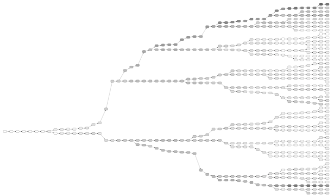
Figure 5: Result of time-lapse microscopy and single cell analysis for the example of one cell lineage tree. Grey color indicates the fluorescence due to mCherry, which is correlated to the amount of plasmids in a cell.

The employed data was derived from a time-lapse microscopy movie of growing Bacillus megaterium cells [22]. These cells were harboring a multi-copy plasmid that contained a xylose-inducible expression system [26]. The main components of this system consist of the xylose repressor gene xylR, the operator region where the XylR protein can bind and a target gene. In presence of xylose the repressor is removed which leads to an induction of expression of the target gene. In the applied plasmid xylR was fused with the mCherry fluorescence gene thus when XylR-mCherry is bound the plasmid is tagged and can be visualized in vivo via fluorescence microscopy. At a sufficient plasmid copy number the signal is high enough to quantify the plasmid abundance in single cells. Using image sequences it is possible to generate time-lapse movies and to follow up plasmid migration and segregation. Spatial and temporal tracking of cells as well as quantification of fluorescence is done by image processing software [15]. The final result is a cell lineage tree (see Figure 5).

We use these data to determine the mode of plasmid replication, and to determine the plasmid transmission characteristics. We intend to validate the model structure and not to do a detailed data analysis; therefore, the parameter are estimated by rather naive methods. Based upon these parameters, the model developed above predicts the plasmid distribution. The model predictions are compared with the experimental data.

Cell and plasmid reproduction.

A first look at the time course of the bacterial and total plasmid population size (we take the sum of all plasmids in all cells) show that plasmid population and cell population both grow exponentially with the same exponent (Figure 6, left panel). This could be a first hint for cell controlled plasmid production (recall the results of section 4.1). We use single cell data to investigate this idea. Surprisingly, a detailed analysis of the increase of plasmids during a cell cycle indicates an almost perfect agreement with an exponential grow (Figure 6, right panel). Therefore we dismiss the hypothesis of cell controlled reproduction in favor of plasmid controlled reproduction. The semi-logarithmic, linear fit reveals for the population growth the exponent $\beta=0.975/h$, and the reproduction rate for plasmids $b_{0}=1.01/h$. The two exponents are almost identical, which is an alternative explanation of the parallel increase of cells and plasmids in the left panel of figure 6. There is no obvious mechanism that couples plasmid- and cell reproduction, though it is rather unlikely that this precise agreement is pure coincidence. We take for the mortality $\mu=0$.

Figure 6: (a) Population dynamics (solid line) and total plasmid content (summarized over all individuals, dashed line). Data: fat lines, exponential fit: thin lines. (b) Exponential fit of the relative plasmid increase between two cell division events.

Transmission characteristics of plasmids from mother to daughter.

As cell-tracking yields information about mother- and daughter cells, we are able to compute the distribution of the relative fraction of plasmids in the two daughters, i.e. we are able to produce a histogram for the kernel density $k(x,1)$. Figure 7 (a) displays this density, together with a best fit of a normal distribution and a fit of a gamma distribution for the cells with more than $1/2$ of the mother’s plasmid, resp. less than $1/2$ of the mother’s plasmids. The gap in the histogram at $1/2$ attracts attention. It is possible to interpret this gap as one indication for an unequal distribution of plasmids between sister cells (see [22] for a more detailed data analysis and discussion). The variance in the distribution is another indication for an unequal plasmid distribution between then two daughter cells.

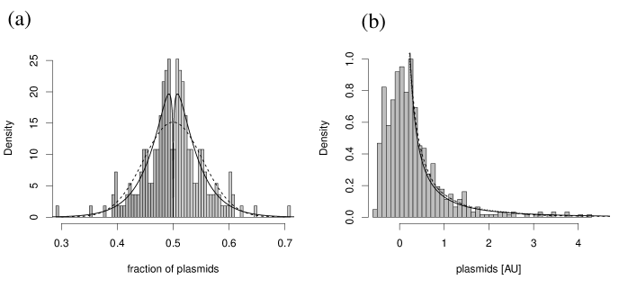
Figure 7: Left panel. Fraction of plasmids in the two daughter cells, together with a normal distribution (dashed line), and two gamma-distributions (solid lines), adapted to the data with more resp. with less than 50% of plasmids. Right panel. Empirical distribution and model-based distribution for three different plasmid transmission kernels (solid: estimated kernel, dashed: symmetric $\delta$-peak, dotted: uniform kernel; note that the solid and the dashed line are almost on top of each other).

Simulation of the data.

We feed these parameter in our population model. To compare the theoretical and the experimental distribution at the end of the experiment (after 4.5 h), we shift the fluorescence distribution by a constant offset to the left, in order to compensate for auto-fluorescence (note that this shift is slightly inconsistent, as the plasmid reproduction rate is determined from the unshifted data); we furthermore rescale the theoretical plasmid distribution with a scalar factor in such a way that the 75% quantile of empirical and simulated distribution agree (see Figure 7). The theoretical and empirical distributions seem to match nicely, in particular if we take into account that the data for low fluorescence are expected to be rather noisy. Other transmission kernels as a $\delta$-peak or a uniform kernel do not affect the outcome essentially. Our model seems to address the most fundamental principles of plasmid- and population dynamics in an appropriate way.
It is interesting to note that $b_{0}=\beta$ does not allow for an integrable equilibrium distribution. We expect a singularity to appear at zero, and (as the average number of plasmids per cell is constant) at the same time few cells to increase infinitely the number of plasmids they inherit. This observation may correlate with experimental observations of many cells with few plasmids, and few cells that accumulate plasmids.

7 Discussion

In this paper, we developed a model for plasmid dynamics in a bacterial population, based on ideas developed in [1]. Using a continuum limit, we obtained the fragmentation equation, as e.g. proposed in [24]. The special structure of our model allowed to convert the hyperbolic partial differential equation into an infinite set of ordinary differential equations for the moments. We then turned to investigate the shape of the equilibrium distributions of plasmids in dependence on different plasmid reproduction modes and plasmid transmission kernels. We defined two fundamental different plasmid reproduction modes: cell controlled production (a cell produces plasmids at a fairly constant rate, that is only decreased due to the plasmid load) and plasmid controlled reproduction (logistic growth). Kuo et al. [16] name the latter mode mass-controlled production, and also introduce a third mode, the “division-controlled mode”. In the “division-controlled mode” cells duplicate plasmids during cell division, such that all daughter cells have – from birth on– the same amount of plasmids as the mother. From the dynamical point of view, this mode is less interesting.
The analysis of the model indicates that the plasmid reproduction mode (production of plasmids per cell or reproduction of plasmids per plasmid) mainly influences the shape of the distribution at few plasmids, while the plasmid reproduction velocity mainly influences the distribution at the carrying capacity of a cell: We expect a pole of the distribution at zero plasmids in the plasmid controlled reproduction mode and that the distribution becomes small at small plasmid numbers for the cell controlled reproduction mode. At the carrying capacity, we expect the distribution to tend to zero if the plasmid reproduction rate is small in comparison with the cell reproduction rate, and to tend to infinity in the other case.

Our results hint that the exact transmission mechanism of plasmids from mother to daughter is only influential if it is distinctively unequal and plasmid reproduction is in the same range as cell reproduction. As the analysis of experimental data revealed, the latter requirement is given in biologically relevant systems. In all other cases, the plasmid segregation mode only leads to a minor correction in the shape of the equilibrium distribution. This finding is an indication that the accumulation of plasmids observed in experiments is not solely due to unequal plasmid segregation, but also due to the interplay of plasmid reproduction and cell reproduction. We expect in particular that cells with a higher plasmid load will reproduce less fast and, in this way, plasmids may have a longer time to accumulate within a cell. Therefore, these cells will divide even less often. In that, we find a positive feedback loop that offers an second mechanism for accumulation, apart of unequal plasmid segregation.

Acknowledgements: We thank Lirike Neziraj for intensive discussions. Part of this work was funded by the German Research Foundation (DFG) within the priority program SPP1617 “Phenotypic heterogeneity and sociobiology of bacterial populations”.

References

- [1] W. E. Bentley and O. E. Quiroga. Investigation of subpopulation heterogeneity and plasmid stability in recombinant Escherichia coli via a simple segregated model. Biotech. Bioengin., 42:224–234, 1992.
- [2] C. Berg and A. J. Durán. Some tranformations of Hausdorff moment sequences and harmonic numbers. Canad. J. Math., 57:941–960, 2005.
- [3] V. Calvez, M. Doumic, and P. Gabriel. Self-similarity in a general aggregation–fragmentation problem. application to fitness analysis. J. Math. Pures Appl., 98(1):1–27, Jul 2012.
- [4] F. Campillo, N. Champagnat, and C. Fritsch. Links between deterministic and stochastic approaches for invasion in growth-fragmentation-death models. Journal of Mathematical Biology, 73(6-7):1781–1821, Apr 2016.
- [5] O. Diekmann, H. A. Lauwerier, T. Aldenberg, and J. A. J. Metz. Growth, fission and the stable size distribution. J. Math. Biol., 18:135–148, 1983.
- [6] M. Doumic. Analysis of a population model structured by the cells molecular content. Math. Model. Nat. Phenom., 2:121–152, 2007.
- [7] M. Doumic and P. Gabriel. Eigenelements of a general aggregation-fragmentation model. Math. Models Methods Appl. Sci., 20(05):757–783, 2010.
- [8] R. Durrett. Probability Models for DNA Sequence Evolution. Springer, 2009.
- [9] V. V. Ganusov, A. V. Bril’kov, and N. S. Pechurkin. Mathematical modeling of population dynamics of unstable plasmid-bearing bacterial strains under continuous cultivation in a chemostat. Biophysics, 45:881–887, 2000.
- [10] P. Goss and J. Peccoud. Analysis of the stabilizing effect of ROM on the genetic network controlling COLE1 plasmid replication. Pac. Symp. Biocomp., 4:65–76, 1999.
- [11] I. Gradshteyn and I. Ryzhik. Table of Integrals, Series, and Products. Academic Press, 1980.
- [12] M. Gyllenberg and H. Heijmans. An abstract delay-differential equation modelling size dependent cell growth and division. SIAM J. Math. Anal., 18:74–88, 1987.
- [13] K. Hadeler and K. Dietz. Nonlinear hyperbolic partial differential equations for the dynamics of parasite populations. Computer Maths. Appl., 9:415–430, 1983.
- [14] B. G. Kim and M. L. Shuler. Kinetic analysis of the effects of plasmid multimerization on segregational instability of ColEl type plasmids in Escherichia coli B/r. Biotech. Bioengin., 37:1076–1086, 1991.
- [15] J. Klein, S. Leupold, I. Biegler, R. Biedendieck, R. Münch, and D. Jahn. Tlm-tracker: software for cell segmentation, tracking and lineage analysis in time-lapse microscopy movies. Bioinformatics, 28:2276–2277, 2012.
- [16] H. Kuo and J. D. Keasling. A Monte Carlo simulation of plasmid replication during the bacterial division cycle. Biotech. Bioengin., 52:633–647, 1996.
- [17] A. v. O. M. Acar, J.T. Mettetal. Stochastic switching as a survival strategy in fluctuating environments. Nat. Gen., 40:471– 475, 2007.
- [18] P. Michel. Existence of a solution to the cell division eigenproblem. Math. Models Methods Appl. Sci., 16:1125–1153, 2006.
- [19] S. Million-Weaver and M. Camps. Mechanisms of plasmid segregation: have multicopy plasmids been overlooked? Plasmid, 75:27–36, 2014.
- [20] S. Mischler and J. Scher. Spectral analysis of semigroups and growth-fragmentation equations. Annales de l’Institut Henri Poincare (C) Non Linear Analysis, In press, 2015.
- [21] J. Müller, B. Hense, T. Fuchs, M. Utz, and C. Pötzsche. Bet-hedging in stochastically switching environments. Journal of Theoretical Biology, 336:144 – 157, 2013.
- [22] K. M. Münch, J. Müller, S. Bergmann, S. Heyber, S. Wienecke, R. Biedendieck, R. Münch, and D. Jahn. Unequal plasmid distribution causing population heterogeneity during heterologous protein production in Bacillus megaterium. Applied and Environmental Microbiology, accepted, DOI:10.1128/AEM.00807-15, 2015.
- [23] K. Nordström. Plasmid R1–replication and its control. Plasmid, 55:1–26, 2006.
- [24] B. Perthame. Transport Euqations in Biology. Birkhäuser, 2007.
- [25] B. Perthame and L. Ryzhik. Exponential decay for the fragmentation or cell-division equation. Journal of Differential Equations, 210(1):155–177, Mar 2005.
- [26] S. Stammen, B. K. Müller, C. Korneli, R. Biedendieck, M. Gamer, E. Franco-Lara, and D. Jahn. High-yield intra- and extracellular protein production using bacillus megaterium. Appl Environ Microbiol, 76:4037–4046, 2010.
- [27] D. K. Summers and D. J. Sherratt. Multimerization of high copy number plasmids causes instability: ColEI encodes a determinant essential for plasmid monomerization and stability. Cell, 36:1097–1103, 1984.
- [28] G. Talenti. Recovering a function from a finite number of moments. Inverse Problems, 3:501–517, 1987.
- [29] S. Tavaré. Ancestral inference in population genetics. In J. Picard, editor, Lectures on Probability Theory and Statistics, pages 3–190. Springer, 2004.
- [30] K. Terpe. Overview of bacterial expression systems for heterologous protein production: from molecular and biochemical fundamentals to commercial systems. Appl Microbiol Biotechnol, 72:211–222, 2006.
- [31] G. Wake, A. A. Zaidi, and B. van Brunt. Tumour cell biology and some new non-local calculus. In M. Wakayama, R. Andersson, J. Cheng, Y. Fukumto, R. McKibbin, K. Polthier, T. Takagi, and K.-C. Toh, editors, The impact of applications on mathematics. Proceedings of the Forum of Mathematics for Industry 2013, pages 27–33, 2014.
- [32] A. Zaidi, B. van Bunt, and G. C. Wake. A model for asymmertical cell division. Math. Biosc. Engin., 12:491–501, 2015.