Error analysis of randomized Runge-Kutta methods for differential equations with time-irregular coefficients

Abstract.

This paper contains an error analysis of two randomized explicit Runge-Kutta schemes for ordinary differential equations (ODEs) with time-irregular coefficient functions. In particular, the methods are applicable to ODEs of Carathéodory type, whose coefficient functions are only integrable with respect to the time variable but are not assumed to be continuous. A further field of application are ODEs with coefficient functions that contain weak singularities with respect to the time variable.

The main result consists of precise bounds for the discretization error with respect to the $L^{p}(\Omega;{\mathbb{R}}^{d})$-norm. In addition, convergence rates are also derived in the almost sure sense. An important ingredient in the analysis are corresponding error bounds for the randomized Riemann sum quadrature rule. The theoretical results are illustrated through a few numerical experiments.

1. Introduction

In this paper we investigate the numerical solution of ordinary differential equations by randomized one-step methods. More precisely, let $T\in(0,\infty)$ and let $u\colon[0,T]\to{\mathbb{R}}^{d}$, $d\in{\mathbb{N}}$, denote the exact solution to the initial value problem

(1) $$\begin{split}\begin{cases}\dot{u}(t)&=f(t,u(t)),\quad t\in[0,T],\\ u(0)&=u_{0},\end{cases}\end{split}$$

where $u_{0}\in{\mathbb{R}}^{d}$ is the initial condition. Let us recall that the initial value problem (1) is said to be of Carathéodory type if the measurable coefficient function $f\colon[0,T]\times{\mathbb{R}}^{d}\to{\mathbb{R}}^{d}$ is (locally) integrable with respect to the temporal variable and continuous with respect to the state variable. If $f$ is additionally assumed to fulfill a (local) Lipschitz condition with respect to the state variable, then it is well-known that the initial value problem (1) admits a unique (local) solution $u$. Recall that a measurable mapping $u\colon[0,T]\to{\mathbb{R}}^{d}$ is called a (global) solution to (1) if $u$ is absolutely continuous and satisfies

(2) $$u(t)=u_{0}+\int_{0}^{t}f(s,u(s))\,\mathrm{d}s$$

for any $t\in[0,T]$. In particular, Equation (2) comes implicitly with the assumption that the mapping $[0,T]\ni t\mapsto f(t,u(t))\in{\mathbb{R}}^{d}$ is integrable. For instance, we refer to [17, Chap. I, Thm 5.3].

Our motivation for studying Carathéodory type initial value problems stems from the fact that certain stochastic differential equations [26, 28] or rough differential equations [11] that are driven by an additive noise can be transformed into a problem of the form (1). For instance, let $b\colon{\mathbb{R}}^{d}\to{\mathbb{R}}^{d}$ be Lipschitz continuous and let $v\colon[0,T]\to{\mathbb{R}}^{d}$ be the solution to a rough differential equation of the form

$$\,\mathrm{d}v(t)=b(v(t))\,\mathrm{d}t+\,\mathrm{d}r(t),\quad v(0)=v_{0},$$

where $r\colon[0,T]\to{\mathbb{R}}^{d}$ is a non-smooth but integrable perturbation. Then, the mapping $u\colon[0,T]\to{\mathbb{R}}^{d}$ given by $u(t):=v(t)-r(t)$, $t\in[0,T]$, solves an ODE of the form (1) with $f(t,x):=b(r(t)+x)$ for each $(t,x)\in[0,T]\times{\mathbb{R}}^{d}$. Depending on the smoothness of the perturbation $r$, the resulting mapping $f$ is then often only integrable or Hölder continuous with exponent $\gamma\in(0,1]$ with respect to the temporal variable $t$.

Due to the low regularity of the coefficient function $f$ the numerical approximation of the solution $u$ to Carathéodory type differential equations is a challenging task. Indeed, it can be shown that any deterministic numerical one-step method is in general divergent if it only uses finitely many point evaluations of $f$. This is easily seen from a simple adaptation of arguments presented in [27, Kap. 2.3]. We discuss this aspect in more depth in Section 1.1 below.

If the coefficient function $f$ enjoys slightly more regularity with respect to the temporal variable, say Hölder continuous with some exponent $\gamma\in(0,1]$ (compare with Assumption 5.1 further below), then classical deterministic numerical algorithms such as Runge-Kutta methods or linear multi-step methods become applicable and will converge to the exact solution. However, since $f$ is not assumed to be differentiable we cannot expect high order of convergence from these schemes. In fact, in [21] it is shown that if $\gamma=1$ then the minimum error of any deterministic method depending only on $N\in{\mathbb{N}}$ point evaluations of the coefficient function $f$ is of order $\mathcal{O}(N^{-1})$. Similarly, for arbitrary values of $\gamma\in(0,1)$ the minimum error among all deterministic algorithms that use at most $N\in{\mathbb{N}}$ point evaluations of $f$ decays only with order $\mathcal{O}(N^{-\gamma})$, see [19]. Therefore, especially in the case of small values for $\gamma$, deterministic methods may still be considered as impracticable.

For these reasons it is necessary to extend the class of considered numerical algorithms. For instance, the method could additionally make use of linear functionals of the coefficient function $f$, say integrals, instead of mere point evaluations. However, it is often not clear how to implement these methods if $f$ is not (piecewise) continuous. Here, we therefore follow a different path that considers randomized numerical methods. The prototype of this class of numerical algorithms is the classical Monte Carlo method, which converges already under an integrability condition.

In the literature, several randomized numerical methods have been developed for the specific initial value problem (1) under a variety of mild regularity assumptions. For instance, we mention the results in [7, 19, 20, 22, 30, 31] and the references therein. These randomized methods are usually found to be superior over corresponding deterministic methods in the sense that the resulting discretization error decays already with order $\mathcal{O}(N^{-\gamma-\frac{1}{2}})$ under the same smoothness assumptions as sketched above. Let us also mention that a further application of randomized methods to initial value problems in Banach spaces is found in [8, 18], while the approximation of stochastic ODEs by a randomized Euler-Maruyama method is considered in [29]. In [6] a related family of quasi-randomized methods is studied.

In this paper we present a precise error analysis for two randomized Runge-Kutta methods that are applicable to the numerical solution of ODEs with time-irregular coefficient functions. The purpose is to prove convergence of the two methods with an order of at least $\frac{1}{2}$ with respect to the $L^{p}(\Omega;{\mathbb{R}}^{d})$-norm under very mild conditions on the coefficient function $f$. Hereby we relax several conditions on $f$ often found in the literature. In particular, we do not assume that the coefficient function is (locally) bounded which allows to treat functions $f$ with a weak singularity of the form $|t-t_{0}|^{-\frac{1}{p}+\epsilon}$, $p\in[2,\infty)$, $\epsilon\in(0,\infty)$, $t,t_{0}\in[0,T]$. In addition, we also estimate the order of convergence in the almost sure sense. The precise conditions on the coefficient function are stated in Assumption 4.1 and Assumption 5.1.

We now introduce the two randomized Runge-Kutta methods in more detail. If the reader is not familiar with standard notations and concepts in probability we suggest to first consult Section 2.

Let $(\tau_{j})_{j\in{\mathbb{N}}}$ be a sequence of independent and $\mathcal{U}(0,1)$-distributed random variables on a probability space $(\Omega,{\mathcal{F}},{\mathbb{P}})$. Then, for any step size $h\in(0,1)$ we define $N_{h}\in{\mathbb{N}}$ to be the integer determined by $N_{h}h\leq T<(N_{h}+1)h$. Set $t_{j}=jh$ for every $j\in{\mathbb{N}}\cup\{0\}$. The first numerical approximation $(U^{j})_{j\in\{0,\ldots,N_{h}\}}$ of $u$ considered in this paper is determined by setting $U^{0}=u_{0}$ and by the recursion

(3) $$\begin{split}U^{j}&=U^{j-1}+hf(t_{j-1}+\tau_{j}h,U^{j-1}),\end{split}$$

for all $j\in\{1,\ldots,N_{h}\}$. This method is usually termed randomized Euler method and it is a particular case of a Runge-Kutta Monte Carlo method studied in [20, 30, 31]. Let us emphasize that, as it is customary for Monte Carlo methods, the result of the numerical scheme is a discrete time stochastic process defined on the same probability space as the random input $(\tau_{j})_{j\in{\mathbb{N}}}$.

The second randomized Runge-Kutta method $(V^{j})_{j\in\{0,\ldots,N_{h}\}}$ is determined by setting $V^{0}=u_{0}$ and by the recursion

(4) $$\begin{split}V^{j}_{\tau}&=V^{j-1}+h\tau_{j}f(t_{j-1},V^{j-1}),\\ V^{j}&=V^{j-1}+hf(t_{j-1}+\tau_{j}h,V^{j}_{\tau}),\end{split}$$

for all $j\in\{1,\ldots,N_{h}\}$. This scheme is a member of a family of methods that has been introduced in [7, 19].

The two methods (3) and (4) can indeed be interpreted as randomized Runge-Kutta methods. In fact, in the $j$-th step of (3) and (4) we randomly choose one particular Runge-Kutta method from the families with Butcher tableaux

(10) $$\begin{array}[]{c|c}\theta&0\\ \hline\cr&1\end{array}, \quad\begin{array}[]{c|cc}0&0&0\\ \theta&\theta&0\\ \hline\cr&0&1\end{array},$$ or

respectively, where the value of the parameter $\theta\in[0,1]$ is determined by the outcome of the random variable $\tau_{j}$. For more details on Runge-Kutta methods and their Butcher-tableaux [3] we refer to standard references, for example [4, 12, 16].

The remainder of this paper is organized as follows. In Section 2 we introduce our notation and recall some prerequisites from probability that are needed later. In Section 3 we state and prove precise error estimates for the randomized Riemann sum quadrature rule, which are an important ingredient in our error analysis for the randomized Runge-Kutta methods (3) and (4). Randomized quadrature rules are well-known to the literature, see [14, 15]. However, this is apparently the first time they are applied in the error analysis of randomized Runge-Kutta methods.

Section 4 contains the first main result of this paper. Here we prove that the randomized Euler method (3) converges to the exact solution of a Carathéodory type ODE (1) with order $\frac{1}{2}$ with respect to the norm in $L^{p}(\Omega;{\mathbb{R}}^{d})$. See Assumption 4.1 for a precise statement of the conditions on the coefficient function $f$. In addition we also derive the order of convergence in the almost sure sense, hereby generalizing results from [20] to unbounded coefficient functions. Note that the computationally more expensive method (4) does not offer any additional advantages in terms of convergence speed in case of possibly discontinuous coefficient functions. We therefore omit an error analysis in this situation.

In Section 5 we then consider the classical ODE setting with a Hölder continuous coefficient function $f$. We determine the order of convergence of the two numerical methods in dependence of the Hölder exponent $\gamma$ and with respect to the $L^{p}(\Omega;{\mathbb{R}}^{d})$-norm. We see that the randomized Runge-Kutta method (4) is superior to the randomized Euler method (3) if $\gamma\in(\frac{1}{2},1]$. These results generalize the error analysis from [7, 19] to the case $p>2$. Since they are based on the $L^{p}$-convergence result, we believe that our almost sure convergence rates are new to the literature as well. Lastly, we present several numerical experiments in the final section.

1.1. Divergence of deterministic algorithms

As announced in the introduction let us briefly follow a line of arguments from [27, Kap. 2.3]. Our aim is to give a sketch of proof that all deterministic algorithms that only use point evaluations of $f$ will in general diverge if applied to Carathéodory type ODEs.

To this end, let $T=1$, $d=1$, and $u_{0}=0$ and consider the problem (1) with the coefficient function $f_{1}(t,x)\equiv 1$ for all $t\in[0,T]$ and $x\in{\mathbb{R}}$. Clearly, in this case the exact solution $u_{1}$ satisfies $u_{1}(1)=1$. If we apply an arbitrary but fixed deterministic algorithm for the approximation of $u_{1}(1)$ with $N\in{\mathbb{N}}$ evaluations of $f_{1}$ it will return an approximation $U_{N}\in{\mathbb{R}}$. Let us assume that for the computation of $U_{N}$ the deterministic algorithm evaluated the coefficient function $f_{1}$ at the points $(t_{i}^{N},x_{i}^{N})\in[0,T]\times{\mathbb{R}}$, $i=1,\ldots,N$, in the extended phase space. For each number $N\in{\mathbb{N}}$ define now the set $B_{N}=\cup_{i=1}^{N}\{t_{i}^{N}\}\subset[0,T]$ as well as $B:=\cup_{n\in{\mathbb{N}}}B_{n}\subset[0,T]$.

Then, we consider a further initial value problem with the same initial condition $u_{0}$ but with the coefficient function $f_{2}(t,x):=\mathbb{I}_{B}(t)$ for all $(t,x)\in[0,T]\times{\mathbb{R}}$. Obviously, the mapping $f_{2}$ is also measurable and bounded. Since $f_{2}$ does not depend on the state variable, it also fits into the framework of Carathéodory type ODEs. In fact, the mapping $f_{2}$ fulfills all conditions of Assumption 4.1 further below. Because the set $B$ has Lebesgue measure zero the exact solution $u_{2}$ satisfies $u_{2}(1)=0$ in this case. However, if we now apply the same deterministic algorithm as above, it cannot distinguish between $f_{1}$ and $f_{2}$ and it will return the same numerical approximation $U_{N}\in{\mathbb{R}}$. Since this is true for any $N\in{\mathbb{N}}$ and since $u_{1}(1)=1\neq 0=u_{2}(1)$ the deterministic algorithm will not converge to the exact solution of at least one of the problems.

2. Preliminaries

In this section we collect a few important results and inequalities in particular from probability, which are needed later. But first we fix some notation and terminology that is frequently used throughout this paper.

As usual we denote by ${\mathbb{N}}$ the set of all positive integers and ${\mathbb{N}}_{0}={\mathbb{N}}\cup\{0\}$, while ${\mathbb{R}}$ denotes the set of all real numbers. By $|\cdot|$ we denote the standard norm on the Euclidean space ${\mathbb{R}}^{d}$, $d\in{\mathbb{N}}$. Further, for every $\gamma\in(0,1]$ we denote by $\mathcal{C}^{\gamma}([0,T]):=\mathcal{C}^{\gamma}([0,T];{\mathbb{R}}^{d})$ the set of all $\gamma$-Hölder continuous mappings $g\colon[0,T]\to{\mathbb{R}}^{d}$. Note that the space $\mathcal{C}^{\gamma}([0,T])$ becomes a Banach space if endowed with the Hölder norm

$$\|g\|_{\mathcal{C}^{\gamma}([0,T])}=\sup_{t\in[0,T]}|g(t)|+\sup_{\begin{subarray}{c}t,s\in[0,T]\\ t\neq s\end{subarray}}\frac{|g(t)-g(s)|}{|t-s|^{\gamma}}.$$

In particular, it then holds true that

$$|g(t)-g(s)|\leq\|g\|_{\mathcal{C}^{\gamma}([0,T])}|t-s|^{\gamma},\quad\text{ for all }t,s\in[0,T].$$

The next inequality is a useful tool to bound the error of a numerical approximation. For a proof and more general variants see for instance Proposition 4.1 in [9].

Lemma 2.1 (Discrete Gronwall’s inequality).

Consider two nonnegative sequences $(u_{n})_{n\in{\mathbb{N}}}$ and $(w_{n})_{n\in{\mathbb{N}}}$ which for some given $a\in[0,\infty)$ satisfy

$$u_{n}\leq a+\sum_{j=1}^{n-1}w_{j}u_{j},\quad\text{ for all }n\in{\mathbb{N}},$$

then for all $n\in{\mathbb{N}}$ it also holds true that

$$u_{n}\leq a\exp\Big{(}\sum_{j=1}^{n-1}w_{j}\Big{)}.$$

For the introduction and the error analysis of Monte Carlo methods, we also require some fundamental concepts from probability and stochastic analysis. For a general introduction readers are referred to standard monographs on this topic, for instance [23, 24, 28]. For the measure theoretical background see [1, 5].

First let us recall that a probability space $(\Omega,\mathcal{F},{\mathbb{P}})$ consists of a measurable space $(\Omega,\mathcal{F})$ endowed with a finite measure ${\mathbb{P}}$ satisfying ${\mathbb{P}}(\Omega)=1$. The value ${\mathbb{P}}(A)\in[0,1]$ is interpreted as the probability of the event $A\in{\mathcal{F}}$. A mapping $X\colon\Omega\to{\mathbb{R}}^{d}$ is called a random variable if $X$ is ${\mathcal{F}}/\mathcal{B}({\mathbb{R}}^{d})$-measurable, where $\mathcal{B}({\mathbb{R}}^{d})$ denotes the Borel-$\sigma$-algebra generated by the set of all open subsets of ${\mathbb{R}}^{d}$. More precisely, it holds true that

$$X^{-1}(B)=\big{\{}\omega\in\Omega\,:\,X(\omega)\in B\big{\}}\in\mathcal{F}$$

for all $B\in\mathcal{B}({\mathbb{R}}^{d})$. Every random variable induces a probability measure on its image space. In fact, the measure $\mu_{X}\colon\mathcal{B}({\mathbb{R}}^{d})\to[0,1]$ given by $\mu_{X}(B)={\mathbb{P}}(X^{-1}(B))$ for all $B\in\mathcal{B}({\mathbb{R}}^{d})$ is a probability measure on the measurable space $({\mathbb{R}}^{d},\mathcal{B}({\mathbb{R}}^{d}))$. Usually, $\mu_{X}$ is called the distribution of $X$.

In this paper, we frequently encounter a family of $\mathcal{U}(a,b)$-distributed random variables $(\tau_{j})_{j\in{\mathbb{N}}}$. This means that for each $j\in{\mathbb{N}}$ the real-valued mapping $\tau_{j}\colon\Omega\to{\mathbb{R}}$ is a random variable which is uniformly distributed on the interval $(a,b)$ with $a,b\in{\mathbb{R}}$, $a<b$. In particular, the distribution $\mu_{\tau_{j}}$ of $\tau_{j}$ is given by $\mu_{\tau_{j}}(A)=\frac{1}{(b-a)}\lambda\big{(}A\cap(a,b)\big{)}$, where $\lambda$ denotes the Lebesgue measure on the real line.

Next, let us recall that a random variable $X\colon\Omega\to{\mathbb{R}}^{d}$ is called integrable if $\int_{\Omega}|X(\omega)|\,\mathrm{d}{\mathbb{P}}(\omega)<\infty$. Then, the expectation of $X$ is defined as

$${\mathbb{E}}[X]:=\int_{\Omega}X(\omega)\,\mathrm{d}{\mathbb{P}}(\omega)=\int_{{\mathbb{R}}^{d}}x\,\mathrm{d}\mu_{X}(x).$$

Moreover, we write $X\in L^{p}(\Omega;{\mathbb{R}}^{d})$ with $p\in[1,\infty)$ if $\int_{\Omega}|X(\omega)|^{p}\,\mathrm{d}{\mathbb{P}}(\omega)<\infty$. In addition, the set $L^{p}(\Omega;{\mathbb{R}}^{d})$ becomes a Banach space if we identify all random variables which only differ on a set of measure zero (i.e. probability zero) and if we endow $L^{p}(\Omega;{\mathbb{R}}^{d})$ with the norm

$$\|X\|_{L^{p}(\Omega;{\mathbb{R}}^{d})}=\big{(}{\mathbb{E}}\big{[}|X|^{p}\big{]}\big{)}^{\frac{1}{p}}=\Big{(}\int_{\Omega}|X(\omega)|^{p}\,\mathrm{d}{\mathbb{P}}(\omega)\Big{)}^{\frac{1}{p}}.$$

This definition coincides with the definition of the standard spaces $L^{p}([0,T];{\mathbb{R}}^{d})$ of $p$-fold Lebesgue-integrable measurable functions. If $X\in L^{p}(\Omega;{\mathbb{R}}^{d})$ for some $p\in[1,\infty)$ the Chebyshev inequality yields for all $\lambda\in(0,\infty)$

(11) $${\mathbb{P}}\big{(}\{\omega\in\Omega\,:\,|X(\omega)|>\lambda\}\big{)}\leq\|X\|^{p}_{L^{p}(\Omega;{\mathbb{R}}^{d})}\lambda^{-p}.$$

Further, we say that a family of ${\mathbb{R}}^{d}$-valued random variables $(X_{n})_{n\in{\mathbb{N}}}$ is independent if for any finite subset $M\subset{\mathbb{N}}$ and for arbitrary events $(A_{m})_{m\in M}\subset\mathcal{B}({\mathbb{R}}^{d})$ we have the multiplication rule

$${\mathbb{P}}\Big{(}\bigcap_{m\in M}\{\omega\in\Omega\,:\,X_{m}(\omega)\in A_{m}\}\Big{)}=\prod_{m\in M}{\mathbb{P}}\big{(}\{\omega\in\Omega\,:\,X_{m}(\omega)\in A_{m}\}\big{)}.$$

On the level of the distributions of $(X_{m})_{m\in{\mathbb{N}}}$ this basically means that the joint distribution of each finite subfamily $(X_{m})_{m\in M}$ is equal to the product measure of the single distributions. From this we directly get the multiplication rule for the expectation

(12) $${\mathbb{E}}\Big{[}\prod_{m\in M}X_{m}\Big{]}=\prod_{m\in M}{\mathbb{E}}\big{[}X_{m}\big{]},$$

provided $X_{m}$ is integrable for each $m\in M$.

If we interpret the index as a time parameter, we say that a family of ${\mathbb{R}}^{d}$-valued random variables $(X_{m})_{m\in{\mathbb{N}}}$ is a discrete time stochastic process. A very important class of stochastic processes are martingales. Without stating a precise definition of martingales it suffices for the understanding of this paper to be aware of the fact that if $(X_{m})_{m\in{\mathbb{N}}}$ is an independent family of integrable random variables satisfying ${\mathbb{E}}[X_{m}]=0$ for each $m\in{\mathbb{N}}$, then the stochastic process defined by the partial sums

$$S_{n}:=\sum_{m=1}^{n}X_{m},\quad n\in{\mathbb{N}},$$

is a discrete time martingale. This enables us to apply powerful inequalities for martingales, such as the following discrete time version of the Burkholder–Davis–Gundy inequality, see [2].

Theorem 2.2 (Burkholder–Davis–Gundy inequality).

For each $p\in(1,\infty)$ there exist positive constants $c_{p}$ and $C_{p}$ such that for every discrete time martingale $(X_{n})_{n\in{\mathbb{N}}}$ and for every $n\in{\mathbb{N}}$ we have

$$c_{p}\|[X]_{n}^{{1}/{2}}\|_{L^{p}(\Omega;{\mathbb{R}})}\leq\big{\|}\max_{j\in\{1,\ldots,n\}}|X_{j}|\big{\|}_{L^{p}(\Omega;{\mathbb{R}})}\leq C_{p}\big{\|}[X]_{n}^{{1}/{2}}\big{\|}_{L^{p}(\Omega;{\mathbb{R}})},$$

where $[X]_{n}=|X_{1}|^{2}+\sum_{k=2}^{n}|X_{k}-X_{k-1}|^{2}$ denotes the quadratic variation of $(X_{n})_{n\in{\mathbb{N}}}$ up to $n$.

Another well-known lemma considers the limiting behaviour of sequences of sets under probability measure (see Theorem 2.7 in [24]).

Lemma 2.3 (Borel-Cantelli Lemma).

If $A_{1},A_{2},\cdots\in\mathcal{F}$ and $\sum_{n=1}^{\infty}{\mathbb{P}}(A_{n})<\infty$, then ${\mathbb{P}}(\limsup_{n\to\infty}A_{n})=0$, where

$$\limsup_{n\to\infty}A_{n}=\bigcap_{n=1}^{\infty}\bigcup_{i=n}^{\infty}A_{i}=\big{\{}\omega\in\Omega\,:\,\omega\in A_{i}\text{ for infinitely many $i\in{\mathbb{N}}$ }\big{\}}.$$

3. Error estimates for randomized Riemann sums

In this section we give precise error estimates for a randomized Riemann sum quadrature rule for integrals whose integrands have various degrees of smoothness. Randomized quadrature rules have been first introduced in [14, 15]. Usually, they consist of a randomized version of classical deterministic quadrature rules and are known to offer advantages if the integrand is not smooth. However, in contrast to most Monte Carlo methods, randomized quadrature rules still suffer from the curse of dimensionality in the same way as their deterministic counter-parts. The main field of application therefore is the numerical approximation of integrals with a non-smooth integrand over a low-dimensional domain. See also [10, Sec. 6.4.5] or [27, Sec. 5.5] for further details.

As in the introduction, for any step size $h\in(0,1)$ we define $N_{h}\in{\mathbb{N}}$ to be the integer determined by $N_{h}h\leq T<(N_{h}+1)h$. Let us recall that for every measurable function $g\colon[0,T]\to{\mathbb{R}}^{d}$ with $\|g\|_{L^{p}([0,T];{\mathbb{R}}^{d})}<\infty$ for some $p\in[2,\infty)$ the randomized Riemann sum approximation $Q_{\tau,h}^{n}[g]$ of $\int_{0}^{t_{n}}g(s)\,\mathrm{d}s$ with step size $h\in(0,1)$ is given by

(13) $$Q_{\tau,h}^{n}[g]:=h\sum_{j=1}^{n}g(t_{j-1}+h\tau_{j}),\quad n\in\{1,\ldots,N_{h}\},$$

where $t_{j}=jh$ and $(\tau_{j})_{j\in{\mathbb{N}}}$ is an independent family of $\mathcal{U}(0,1)$-distributed random variables on a probability space $(\Omega,{\mathcal{F}},{\mathbb{P}})$.

The first theorem contains an error estimate with respect to the $L^{p}(\Omega;{\mathbb{R}}^{d})$-norm. Further below, we also study the almost sure convergence of $Q_{\tau,h}^{n}[g]$.

Theorem 3.1 ($L^{p}$-error estimate).

Let $g\colon[0,T]\to{\mathbb{R}}^{d}$ be a measurable mapping satisfying $\|g\|_{L^{p}([0,T];{\mathbb{R}}^{d})}<\infty$ for some $p\in[2,\infty)$. Then, for every $h\in(0,1)$ and $n\in\{1,\ldots,N_{h}\}$ the randomized Riemann sum $Q_{\tau,h}^{n}[g]\in L^{p}(\Omega;{\mathbb{R}}^{d})$ is an unbiased estimator for the integral $\int_{0}^{t_{n}}g(s)\,\mathrm{d}s$, i.e., ${\mathbb{E}}[Q_{\tau,h}^{n}[g]]=\int_{0}^{t_{n}}g(s)\,\mathrm{d}s$. Further, for all $h\in(0,1)$ we have

(14) $$\Big{\|}\max_{n\in\{1,\ldots,N_{h}\}}\Big{|}\int_{0}^{t_{n}}g(s)\,\mathrm{d}s-Q_{\tau,h}^{n}[g]\Big{|}\,\Big{\|}_{L^{p}(\Omega;{\mathbb{R}})}\leq 2C_{p}T^{\frac{p-2}{2p}}\|g\|_{L^{p}([0,T];{\mathbb{R}}^{d})}h^{\frac{1}{2}}.$$

In addition, if the mapping $g$ is $\gamma$-Hölder continuous for some $\gamma\in(0,1]$, then for all $h\in(0,1)$ we have

(15) $$\Big{\|}\max_{n\in\{1,\ldots,N_{h}\}}\Big{|}\int_{0}^{t_{n}}g(s)\,\mathrm{d}s-Q_{\tau,h}^{n}[g]\Big{|}\,\Big{\|}_{L^{p}(\Omega;{\mathbb{R}})}\leq C_{p}\sqrt{T}\|g\|_{\mathcal{C}^{\gamma}([0,T])}h^{\frac{1}{2}+\gamma}.$$

Proof.

First, due to $\|g\|_{L^{p}([0,T];{\mathbb{R}}^{d})}<\infty$ and $\tau_{j}\sim\mathcal{U}(0,1)$ it follows

(16) $$h\big{\|}g(t_{j-1}+h\tau_{j})\big{\|}_{L^{p}(\Omega;{\mathbb{R}}^{d})}^{p}=\int_{t_{j-1}}^{t_{j}}|g(s)|^{p}\,\mathrm{d}s<\infty.$$

Hence, $Q_{\tau,h}^{n}[g]\in L^{p}(\Omega;{\mathbb{R}}^{d})$. After taking the expected value of $Q_{\tau,h}^{n}[g]$ we get

$${\mathbb{E}}\big{[}Q_{\tau,h}^{n}[g]\big{]} =h\sum_{j=1}^{n}{\mathbb{E}}\big{[}g(t_{j-1}+h\tau_{j})\big{]}=h\sum_{j=1}^{n}\int_{0}^{1}g(t_{j-1}+sh)\,\mathrm{d}s$$

$$=\sum_{j=1}^{n}\int_{t_{j-1}}^{t_{j}}g(s)\,\mathrm{d}s=\int_{0}^{t_{n}}g(s)\,\mathrm{d}s.$$

Thus, the randomized Riemann sum is an unbiased estimator for $\int_{0}^{t_{n}}g(s)\,\mathrm{d}s$. Further, by linearity of the integral we obtain for the error

$$E^{n}:=\int_{0}^{t_{n}}g(s)\,\mathrm{d}s-Q_{\tau,h}^{n}[g] =\sum_{j=1}^{n}\int_{t_{j-1}}^{t_{j}}\big{(}g(s)-g(t_{j-1}+h\tau_{j})\big{)}\,\mathrm{d}s.$$

Now, as above it follows that each summand is a centered random variable, that is

$${\mathbb{E}}\Big{[}\int_{t_{j-1}}^{t_{j}}\big{(}g(s)-g(t_{j-1}+h\tau_{j})\big{)}\,\mathrm{d}s\Big{]}=0$$

for every $j\in{\mathbb{N}}$. Moreover, the summands are mutually independent due to the independence of $(\tau_{j})_{j\in{\mathbb{N}}}$. In addition, we also obtain from (16) that

$$\Big{\|}\int_{t_{j-1}}^{t_{j}}\big{(}g(s)-g(t_{j-1}+h\tau_{j})\big{)}\,\mathrm{d}s\Big{\|}_{L^{p}(\Omega;{\mathbb{R}}^{d})}$$

$$\quad\leq\int_{t_{j-1}}^{t_{j}}|g(s)|\,\mathrm{d}s+h\big{\|}g(t_{j-1}+h\tau_{j})\big{\|}_{L^{p}(\Omega;{\mathbb{R}}^{d})}<\infty.$$

Therefore, $(E^{n})_{n\in\{1,\ldots,N_{h}\}}$ is a discrete time $L^{p}$-martingale. Thus, we can apply the Burkholder-Davis-Gundy inequality from Theorem 2.2 and obtain

$$\big{\|}\max_{n\in\{1,\ldots,N_{h}\}}|E^{n}|\big{\|}_{L^{p}(\Omega;{\mathbb{R}})}\leq C_{p}\big{\|}[E]^{\frac{1}{2}}_{N_{h}}\big{\|}_{L^{p}(\Omega;{\mathbb{R}})}.$$

After inserting the quadratic variation $[E]_{N_{h}}$ we arrive at

(17) $$\begin{split}&\big{\|}\max_{n\in\{1,\ldots,N_{h}\}}|E^{n}|\big{\|}_{L^{p}(\Omega;{\mathbb{R}})}\\ &\quad\leq C_{p}\Big{\|}\Big{(}\sum_{j=1}^{N_{h}}\Big{|}\int_{t_{j-1}}^{t_{j}}\big{(}g(s)-g(t_{j-1}+h\tau_{j})\big{)}\,\mathrm{d}s\Big{|}^{2}\Big{)}^{\frac{1}{2}}\Big{\|}_{L^{p}(\Omega;{\mathbb{R}})}\\ &\quad=C_{p}\Big{\|}\sum_{j=1}^{N_{h}}\Big{|}\int_{t_{j-1}}^{t_{j}}\big{(}g(s)-g(t_{j-1}+h\tau_{j})\big{)}\,\mathrm{d}s\Big{|}^{2}\,\Big{\|}_{L^{\frac{p}{2}}(\Omega;{\mathbb{R}})}^{\frac{1}{2}}\\ &\quad\leq C_{p}\Big{(}\sum_{j=1}^{N_{h}}\Big{\|}\int_{t_{j-1}}^{t_{j}}\big{(}g(s)-g(t_{j-1}+h\tau_{j})\big{)}\,\mathrm{d}s\Big{\|}_{L^{p}(\Omega;{\mathbb{R}}^{d})}^{2}\Big{)}^{\frac{1}{2}}.\end{split}$$

Now, by an application of the triangle inequality we get

$$\big{\|}\max_{n\in\{1,\ldots,N_{h}\}}|E^{n}|\big{\|}_{L^{p}(\Omega;{\mathbb{R}})}$$

$$\quad\leq C_{p}\Big{(}\sum_{j=1}^{N_{h}}\Big{|}\int_{t_{j-1}}^{t_{j}}g(s)\,\mathrm{d}s\Big{|}^{2}\Big{)}^{\frac{1}{2}}+C_{p}\Big{(}\sum_{j=1}^{N_{h}}h^{2}\big{\|}g(t_{j-1}+h\tau_{j})\big{\|}_{L^{p}(\Omega;{\mathbb{R}}^{d})}^{2}\Big{)}^{\frac{1}{2}}.$$

The first term is then bounded by

(18) $$\begin{split}\Big{(}\sum_{j=1}^{N_{h}}\Big{|}\int_{t_{j-1}}^{t_{j}}g(s)\,\mathrm{d}s\Big{|}^{2}\Big{)}^{\frac{1}{2}}&\leq h^{\frac{1}{2}}\Big{(}\sum_{j=1}^{N_{h}}\int_{t_{j-1}}^{t_{j}}\big{|}g(s)\big{|}^{2}\,\mathrm{d}s\Big{)}^{\frac{1}{2}}\leq\|g\|_{L^{2}([0,T];{\mathbb{R}}^{d})}h^{\frac{1}{2}}\\ &\leq T^{\frac{p-2}{2p}}\|g\|_{L^{p}([0,T];{\mathbb{R}}^{d})}h^{\frac{1}{2}},\end{split}$$

since $\|g\|_{L^{2}([0,T];{\mathbb{R}}^{d})}\leq T^{\frac{p-2}{2p}}\|g\|_{L^{p}([0,T];{\mathbb{R}}^{d})}$ by Hölder’s inequality.

If $p=2$ we directly obtain the same bound for the second term by making use of (16). If $p\in(2,\infty)$ we first apply Hölder’s inequality with exponents $\rho=\frac{p}{2}\in(1,\infty)$ and $\rho^{\prime}=\frac{p}{p-2}\in(1,\infty)$. This yields

(19) $$\begin{split}&\sum_{j=1}^{N_{h}}h^{2-\frac{2}{p}}\cdot h^{\frac{2}{p}}\big{\|}g(t_{j-1}+h\tau_{j})\big{\|}_{L^{p}(\Omega;{\mathbb{R}}^{d})}^{2}\\ &\quad\leq\Big{(}\sum_{j=1}^{N_{h}}h^{\rho^{\prime}(2-\frac{2}{p})}\Big{)}^{\frac{1}{\rho^{\prime}}}\Big{(}\sum_{j=1}^{N_{h}}h\big{\|}g(t_{j-1}+h\tau_{j})\big{\|}_{L^{p}(\Omega;{\mathbb{R}}^{d})}^{p}\Big{)}^{\frac{2}{p}}\\ &\quad\leq T^{\frac{1}{\rho^{\prime}}}h^{2(1-\frac{1}{p})-\frac{1}{\rho^{\prime}}}\big{\|}g\big{\|}_{L^{p}([0,T];{\mathbb{R}}^{d})}^{2},\end{split}$$

due to (16). Altogether, since $T^{\frac{1}{2\rho^{\prime}}}=T^{\frac{p-2}{2p}}$ and after noting that $h^{2(1-\frac{1}{p})-\frac{1}{\rho^{\prime}}}=h$ we derive from (17), (18) and (19) that

$$\big{\|}\max_{n\in\{1,\ldots,N_{h}\}}|E^{n}|\big{\|}_{L^{p}(\Omega;{\mathbb{R}})}\leq 2C_{p}T^{\frac{p-2}{2p}}\|g\|_{L^{p}([0,T];{\mathbb{R}}^{d})}h^{\frac{1}{2}}.$$

This completes the proof of (14).

Next, if in addition $g\in\mathcal{C}^{\gamma}([0,T])$, then we can improve the estimate in (17) by

$$\Big{\|}\int_{t_{j-1}}^{t_{j}}\big{(}g(s)-g(t_{j-1}+h\tau_{j})\big{)}\,\mathrm{d}s\Big{\|}_{L^{p}(\Omega;{\mathbb{R}}^{d})}$$

$$\quad\leq\int_{t_{j-1}}^{t_{j}}\big{\|}g(s)-g(t_{j-1}+h\tau_{j})\big{\|}_{L^{p}(\Omega;{\mathbb{R}}^{d})}\,\mathrm{d}s\leq\|g\|_{\mathcal{C}^{\gamma}([0,T])}h^{1+\gamma}.$$

Thus, inserting this into (17) gives

$$\big{\|}\max_{n\in\{0,1,\ldots,N_{h}\}}|E^{n}|\big{\|}_{L^{p}(\Omega;{\mathbb{R}})} \leq C_{p}\Big{(}\sum_{j=1}^{N_{h}}\|g\|_{\mathcal{C}^{\gamma}([0,T])}^{2}h^{2(1+\gamma)}\Big{)}^{\frac{1}{2}}$$

$$\leq C_{p}T^{\frac{1}{2}}\|g\|_{\mathcal{C}^{\gamma}([0,T])}h^{\frac{1}{2}+\gamma}.$$

This completes the proof of (15). ∎

Error estimates with respect to the $L^{p}$-norm are sometimes unsatisfactory, since they allow for the possibility that single realizations of the randomized Riemann sum may differ significantly from its expected value. But in practice often just one realization of the estimator is computed. To some extent this is justified by the next theorem. This indicates that already on the level of single “typical” realizations of $Q_{\tau,h}^{n}[g](\omega)$ we observe convergence provided the step size $h$ is sufficiently small. However, depending on the value of $p\in(2,\infty)$ the order of convergence may be significantly reduced.

Theorem 3.2 (Almost sure convergence).

Let $g\colon[0,T]\to{\mathbb{R}}^{d}$ be a given measurable mapping with $\|g\|_{L^{p}([0,T];{\mathbb{R}}^{d})}<\infty$ for some $p\in(2,\infty)$. Let $(h_{m})_{m\in{\mathbb{N}}}\subset(0,1)$ be an arbitrary sequence of step sizes with $\sum_{m=1}^{\infty}h_{m}<\infty$. Then, there exist a nonnegative random variable $m_{0}\colon\Omega\to{\mathbb{N}}_{0}$ and a measurable set $A\in{\mathcal{F}}$ with ${\mathbb{P}}(A)=1$ such that for all $\omega\in A$ and $m\geq m_{0}(\omega)$ we have

(20) $$\max_{n\in\{0,1,\ldots,N_{h_{m}}\}}\Big{|}\int_{0}^{t_{n}}g(s)\,\mathrm{d}s-Q_{\tau,h_{m}}^{n}[g](\omega)\Big{|}\leq h_{m}^{\frac{1}{2}-\frac{1}{p}}.$$

Moreover, if in addition $g\in\mathcal{C}^{\gamma}([0,T])$ for some $\gamma\in(0,1]$, then for every $\epsilon\in(0,\frac{1}{2})$ there exist a nonnegative random variable $m_{0}^{\epsilon}\colon\Omega\to{\mathbb{N}}_{0}$ and a measurable set $A_{\epsilon}\in{\mathcal{F}}$ with ${\mathbb{P}}(A_{\epsilon})=1$ such that for all $\omega\in A_{\epsilon}$ and $m\geq m_{0}^{\epsilon}(\omega)$ we have

(21) $$\max_{n\in\{0,1,\ldots,N_{h_{m}}\}}\Big{|}\int_{0}^{t_{n}}g(s)\,\mathrm{d}s-Q_{\tau,h_{m}}^{n}[g](\omega)\Big{|}\leq h_{m}^{\frac{1}{2}+\gamma-\epsilon}.$$

For the proof we need the following result, which is a simple consequence of the Borel-Cantelli lemma. It is a version of [25, Lemma 2.1], which in turn is based on a technique developed in [13].

Lemma 3.3.

Let $p\in[1,\infty)$ and $\rho\in(\frac{1}{p},\infty)$ be given. Consider an arbitrary sequence of step sizes $(h_{m})_{m\in{\mathbb{N}}}\subset(0,1)$ with $\sum_{m=1}^{\infty}h_{m}<\infty$. Then, for every sequence $(X_{m})_{m\in{\mathbb{N}}}\subset L^{p}(\Omega;{\mathbb{R}}^{d})$ satisfying

$$\sup_{m\in{\mathbb{N}}}h_{m}^{-\rho}\|X_{m}\|_{L^{p}(\Omega;{\mathbb{R}}^{d})}<\infty,$$

there exist a nonnegative random variable $m_{0}\colon\Omega\to{\mathbb{N}}_{0}$ and a measurable set $A\in{\mathcal{F}}$ with ${\mathbb{P}}(A)=1$ such that for every $\omega\in A$ and $m\geq m_{0}(\omega)$ it holds true that

$$|X_{m}(\omega)|\leq h_{m}^{\rho-\frac{1}{p}}.$$

Proof.

For each $m\in{\mathbb{N}}$ consider the event

$$A_{m}:=\big{\{}\omega\in\Omega\,:\,|X_{m}(\omega)|>h_{m}^{\rho-\frac{1}{p}}\big{\}}\in{\mathcal{F}}.$$

Then, by the Chebyshev inequality (11) it holds true that

$${\mathbb{P}}(A_{m}) \leq\|X_{m}\|^{p}_{L^{p}(\Omega;{\mathbb{R}}^{d})}h_{m}^{1-p\rho}$$

for all $m\in{\mathbb{N}}$. Consequently,

$$\sum_{m=1}^{\infty}{\mathbb{P}}(A_{m})\leq\sum_{m=1}^{\infty}\|X_{m}\|^{p}_{L^{p}(\Omega;{\mathbb{R}}^{d})}h_{m}^{1-p\rho}\leq\sup_{j\in{\mathbb{N}}}\Big{(}h_{j}^{-p\rho}\|X_{j}\|^{p}_{L^{p}(\Omega;{\mathbb{R}}^{d})}\Big{)}\sum_{m=1}^{\infty}h_{m}<\infty$$

due to our assumptions on $(X_{m})_{m\in{\mathbb{N}}}$ and $(h_{m})_{m\in{\mathbb{N}}}$. Thus, the Borel-Cantelli lemma (see Lemma 2.3) yields ${\mathbb{P}}(\limsup_{m\to\infty}A_{m})=0$. Since

$$\limsup_{m\to\infty}A_{m} =\big{\{}\omega\in\Omega\,:\,|X_{m}(\omega)|>h_{m}^{\rho-\frac{1}{p}}\text{ for infinitely many }m\in{\mathbb{N}}\big{\}}$$

the assertion follows with $A\in{\mathcal{F}}$ being the complement of $\limsup_{m\to\infty}A_{m}\in{\mathcal{F}}$. Finally, the random variable $m_{0}\colon\Omega\to{\mathbb{N}}_{0}$ is defined by

$$m_{0}(\omega):=\max\big{(}\{1\}\cup\big{\{}m\in{\mathbb{N}}\,:\,|X_{m}(\omega)|>h_{m}^{\rho-\frac{1}{p}}\big{\}}\big{)}<\infty,\quad\text{ for all }\omega\in A,$$

and $m_{0}(\omega)=0$ for all $\omega\in\Omega\setminus A$. ∎

Remark 3.4.

The result of Lemma 3.3 can equivalently be reformulated as follows: Under the same assumptions there exist a measurable set $A\in{\mathcal{F}}$ with ${\mathbb{P}}(A)=1$ and a nonnegative random variable $M\in L^{p}(\Omega;{\mathbb{R}})$ such that for all $m\in{\mathbb{N}}$ and $\omega\in A$ we have

$$|X_{m}(\omega)|\leq M(\omega)h_{m}^{\rho-\frac{1}{p}}.$$

Hence, it is possible to relax the $\omega$-dependent step size restriction in Lemma 3.3 in form of the random variable $m_{0}$ on the cost of introducing an $\omega$-dependent error constant $M(\omega)$. For further details we refer to the proof of [25, Lemma 2.1].

The proof of Theorem 3.2 is now a simple consequence of Theorem 3.1 and Lemma 3.3:

Proof of Theorem 3.2.

First, we assume that $g\in L^{p}([0,T];{\mathbb{R}}^{d})$ for some $p\in(2,\infty)$. Let $(h_{m})_{m\in{\mathbb{N}}}$ be an arbitrary sequence of step sizes with $\sum_{m=1}^{\infty}h_{m}<\infty$. Then define

$$X_{m}:=\max_{n\in\{1,\ldots,N_{h_{m}}\}}\Big{|}\int_{0}^{t_{n}}g(s)\,\mathrm{d}s-Q_{\tau,h_{m}}^{n}[g]\Big{|}$$

Clearly, $X_{m}\in L^{p}(\Omega;{\mathbb{R}})$ for each $m\in{\mathbb{N}}$. In particular, from (14) it follows that

$$\|X_{m}\|_{L^{p}(\Omega;{\mathbb{R}})}\leq 2C_{p}T^{\frac{p-2}{2p}}\|g\|_{L^{p}(\Omega;{\mathbb{R}})}h_{m}^{\frac{1}{2}}.$$

Thus, since $p>2$ the conditions of Lemma 3.3 are fulfilled with $\rho=\frac{1}{2}$ and assertion (20) follows directly.

Next, if we additionally assume that $g\in\mathcal{C}^{\gamma}([0,T])$ for some $\gamma\in(0,1]$ then we immediately have $g\in L^{p}([0,T];{\mathbb{R}}^{d})$ for every $p\in[2,\infty)$. Let $\epsilon\in(0,\frac{1}{2})$ be arbitrary. Choose a value for $p\in(2,\infty)$ such that $\frac{1}{p}<\epsilon$. Then, if we define $X_{m}$ as above we obtain from (15) that

$$\|X_{m}\|_{L^{p}(\Omega;{\mathbb{R}})}\leq C_{p}\sqrt{T}\|g\|_{\mathcal{C}^{\gamma}([0,T])}h_{m}^{\frac{1}{2}+\gamma}$$

for every $m\in{\mathbb{N}}$. Thus, a further application of Lemma 3.3 with $\rho=\frac{1}{2}+\gamma$ yields

$$|X_{m}(\omega)|\leq h_{m}^{\frac{1}{2}+\gamma-\frac{1}{p}}\leq h_{m}^{\frac{1}{2}+\gamma-\epsilon}$$

for all $m\geq m_{0}^{\epsilon}(\omega)$ with probability one. ∎

4. Numerical approximation of Carathéodory ODEs

In this section we investigate the numerical approximation of the exact solution $u$ to the Carathéodory type ordinary differential equation (1). In particular, we derive the order of convergence of the randomized Euler method (3) with respect to the norm in $L^{p}(\Omega;{\mathbb{R}}^{d})$. We also state the order of convergence in the almost sure sense. Throughout this section, we shall allow the following assumptions on the coefficient function $f$.

Assumption 4.1.

The coefficient function $f\colon[0,T]\times{\mathbb{R}}^{d}\to{\mathbb{R}}^{d}$ is assumed to be measurable. Further, there exist $p\in[1,\infty]$ and a measurable mapping $L\colon[0,T]\to[0,\infty)$ with $\|L\|_{L^{p}([0,T];{\mathbb{R}})}<\infty$ such that

(22) $$|f(t,x_{1})-f(t,x_{2})| \leq L(t)|x_{1}-x_{2}|$$

for almost all $t\in[0,T]$ and $x_{1},x_{2}\in{\mathbb{R}}^{d}$. In addition, there is a measurable mapping $K\colon[0,T]\to[0,\infty)$ with $\|K\|_{L^{p}([0,T];{\mathbb{R}})}<\infty$ such that

(23) $$|f(t,0)|\leq K(t)$$

for almost all $t\in[0,T]$.

Let us stress, that the mapping $f$ is not necessarily continuous with respect to the temporal variable $t$. In addition, the mappings $L$ and $K$ are not assumed to be bounded, in contrast to other results found in the literature [6, 20, 30, 31]. Moreover, from (22) and (23) we directly deduce the linear growth condition

(24) $$|f(t,x)|\leq\overline{K}(t)(1+|x|)$$

for almost all $t\in[0,T]$ and $x\in{\mathbb{R}}^{d}$. Here, $\overline{K}\colon[0,T]\to[0,\infty)$ is the $L^{p}$-integrable mapping determined by $\overline{K}(t):=\max(K(t),L(t))$, $t\in[0,T]$. Assumption 4.1 is more than sufficient to ensure the existence of a unique solution $u$ to the initial value problem (1), see [17, Chap. I, Thm 5.3].

In the following proposition we collect a few properties of the solution $u$ to (1).

Proposition 4.2.

Let Assumption 4.1 be fulfilled with $p\in[1,\infty]$. Then, the solution $u$ to the initial value problem (1) satisfies

(25) $$|u(t)|\leq\Big{(}|u_{0}|+\int_{0}^{T}\overline{K}(s)\,\mathrm{d}s\Big{)}\exp\Big{(}\int_{0}^{t}\overline{K}(s)\,\mathrm{d}s\Big{)},\quad t\in[0,T].$$

Moreover, if $p\in(1,\infty]$ then for any $0\leq s\leq t\leq T$ it holds true that

(26) $$|u(t)-u(s)|\leq\|\overline{K}\|_{L^{p}([0,T];{\mathbb{R}})}\Big{(}1+\sup_{z\in[0,T]}|u(z)|\Big{)}|t-s|^{1-\frac{1}{p}}.$$

In particular, $u$ is Hölder continuous with exponent $(1-\frac{1}{p})>0$.

Proof.

Let $u$ be the solution to (1). Then, from (2) and (24) we get that

$$|u(t)| \leq|u_{0}|+\int_{0}^{t}|f(s,u(s))|\,\mathrm{d}s$$

$$\leq|u_{0}|+\int_{0}^{t}\overline{K}(s)(1+|u(s)|)\,\mathrm{d}s$$

$$\leq|u_{0}|+\int_{0}^{T}\overline{K}(s)\,\mathrm{d}s+\int_{0}^{t}\overline{K}(s)|u(s)|\,\mathrm{d}s.$$

Then, an application of Gronwall’s inequality (see e.g. [17, Chap. I, Cor. 6.6]) yields the assertion (25).

Next, assume that $p\in(1,\infty)$ and let $0\leq s\leq t\leq T$ be arbitrary. Then, from (2) and (24) we further deduce that

$$|u(t)-u(s)| \leq\int_{s}^{t}|f(z,u(z))|\,\mathrm{d}z\leq\int_{s}^{t}\overline{K}(z)(1+|u(z)|)\,\mathrm{d}z.$$

Since $u$ is bounded and since the mapping $\overline{K}$ is $p$-fold integrable we obtain from the Hölder inequality with exponents $p$ and $p^{\prime}=\frac{p}{p-1}\in(1,\infty)$ that

$$|u(t)-u(s)| \leq\int_{0}^{T}\mathbb{I}_{[s,t]}(z)\overline{K}(z)(1+|u(z)|)\,\mathrm{d}z$$

$$\leq\Big{(}1+\sup_{z\in[0,T]}|u(z)|\Big{)}\Big{(}\int_{0}^{T}\overline{K}(z)^{p}\,\mathrm{d}z\Big{)}^{\frac{1}{p}}|t-s|^{\frac{1}{p^{\prime}}}$$

Due to $\frac{1}{p^{\prime}}=1-\frac{1}{p}$ this proves the asserted Hölder continuity of $u$ if $p\in(1,\infty)$. The case $p=\infty$ is treated similarly. ∎

Now we are well prepared to state the main result of this section. The following theorem provides an error estimate of the randomized Euler method (3) under Assumption 4.1 with respect to the norm in $L^{p}(\Omega;{\mathbb{R}}^{d})$. We give an explicit expression for the error constant further below.

Theorem 4.3 ($L^{p}$-error estimate).

Let Assumption 4.1 be fulfilled with $p\in[2,\infty)$. Let $u$ denote the exact solution to (1). For given $h\in(0,1)$ let $(U^{j})_{j\in\{0,1,\ldots,N_{h}\}}$ denote the numerical approximation determined by (3) with initial condition $U^{0}=u_{0}$. Then, there exists $C\in(0,\infty)$, independent of $h\in(0,1)$, such that

$$\big{\|}\max_{n\in\{0,1,\ldots,N_{h}\}}|u(t_{n})-U^{n}|\big{\|}_{L^{p}(\Omega;{\mathbb{R}})}\leq Ch^{\frac{1}{2}}.$$

Proof.

Let $h\in(0,1)$ and $n\in\{1,\ldots,N_{h}\}$ be arbitrary. Since $U^{0}=u_{0}$ and by using a telescopic sum argument as well as (2) and (3) and we get

$$u(t_{n})-U^{n} =u(0)-U^{0}+\sum_{j=1}^{n}\big{(}u(t_{j})-u(t_{j-1})-(U^{j}-U^{j-1})\big{)}$$

$$=\sum_{j=1}^{n}\Big{(}\int_{t_{j-1}}^{t_{j}}f(s,u(s))\,\mathrm{d}s-hf(t_{j-1}+\tau_{j}h,U^{j-1})\Big{)}.$$

In order to simplify the notation we write $\theta_{j}:=t_{j-1}+\tau_{j}h$. Note that the family of random variables $(\theta_{j})_{j\in{\mathbb{N}}}$ is independent and $\theta_{j}$ is uniformly distributed on the interval $[t_{j-1},t_{j}]$ for each $j\in\{1,\ldots,N_{h}\}$. Then, after adding and subtracting several terms we have to estimate the following three sums

(27) $$\begin{split}u(t_{n})-U^{n}&=\sum_{j=1}^{n}\Big{(}\int_{t_{j-1}}^{t_{j}}f(s,u(s))\,\mathrm{d}s-hf(\theta_{j},u(\theta_{j}))\Big{)}\\ &\quad+h\sum_{j=1}^{n}\Big{(}f\big{(}\theta_{j},u(\theta_{j})\big{)}-f\big{(}\theta_{j},u(t_{j-1})\big{)}\Big{)}\\ &\quad+h\sum_{j=1}^{n}\Big{(}f\big{(}\theta_{j},u(t_{j-1})\big{)}-f\big{(}\theta_{j},U^{j-1}\big{)}\Big{)}\\ &=:S_{1}^{n}+S_{2}^{n}+S_{3}^{n}.\end{split}$$

First, we give an estimate of the term $S_{3}^{n}$. To this end we apply (22) and arrive at

$$|S_{3}^{n}| \leq h\sum_{j=1}^{n}\Big{|}f\big{(}\theta_{j},u(t_{j-1})\big{)}-f\big{(}\theta_{j},U^{j-1}\big{)}\Big{|}$$

$$\leq h\sum_{j=1}^{n}L(\theta_{j})\big{|}u(t_{j-1})-U^{j-1}\big{|}$$

$$\leq h\sum_{j=1}^{n}L(\theta_{j})\max_{i\in\{0,1,\ldots,j-1\}}\big{|}u(t_{i})-U^{i}\big{|}.$$

Observe that this inequality is only valid in the almost sure sense, since (22) holds for almost all $t\in[0,T]$. However, this is sufficient, since the expected value will eventually be applied. Therefore, after taking the Euclidean norm $|\cdot|$ and the maximum over the time levels in (27) we obtain

$$\max_{i\in\{0,1,\ldots,n\}}\big{|}u(t_{i})-U^{i}\big{|} \leq\max_{j\in\{1,\ldots,N_{h}\}}|S_{1}^{j}|+\max_{j\in\{1,\ldots,N_{h}\}}|S_{2}^{j}|$$

$$\quad+h\sum_{j=1}^{n}L(\theta_{j})\max_{i\in\{0,1,\ldots,j-1\}}\big{|}u(t_{i})-U^{i}\big{|}$$

almost surely for every $n\in\{1,\ldots,N_{h}\}$. Next, we apply the $p$-th power of the $L^{p}(\Omega;{\mathbb{R}})$-norm to both sides of the inequality. From the fact that $(a+b)^{p}\leq 2^{p-1}(a^{p}+b^{p})$ for all $a,b\in[0,\infty)$ we then get

(28) $$\begin{split}&\big{\|}\max_{i\in\{0,1,\ldots,n\}}\big{|}u(t_{i})-U^{i}\big{|}\big{\|}_{L^{p}(\Omega;{\mathbb{R}})}^{p}\\ &\quad\leq 2^{p-1}\big{\|}\max_{n\in\{1,\ldots,N_{h}\}}|S_{1}^{n}|+\max_{n\in\{1,\ldots,N_{h}\}}|S_{2}^{n}|\big{\|}_{L^{p}(\Omega;{\mathbb{R}})}^{p}\\ &\qquad+2^{p-1}\Big{\|}h\sum_{j=1}^{n}L(\theta_{j})\max_{i\in\{0,1,\ldots,j-1\}}\big{|}u(t_{i})-U^{i}\big{|}\Big{\|}_{L^{p}(\Omega;{\mathbb{R}})}^{p}.\end{split}$$

The last term is further estimated by Hölder’s inequality as follows

$$\Big{\|}h\sum_{j=1}^{n}1\cdot L(\theta_{j})\max_{i\in\{0,1,\ldots,j-1\}}\big{|}u(t_{i})-U^{i}\big{|}\Big{\|}_{L^{p}(\Omega;{\mathbb{R}})}^{p}$$

$$\quad\leq h^{p}n^{p-1}\sum_{j=1}^{n}\big{\|}L(\theta_{j})\max_{i\in\{0,1,\ldots,j-1\}}\big{|}u(t_{i})-U^{i}\big{|}\big{\|}_{L^{p}(\Omega;{\mathbb{R}})}^{p}.$$

For the next step, first take note of

(29) $${\mathbb{E}}\big{[}L(\theta_{j})^{p}\big{]}=\frac{1}{h}\int_{t_{j-1}}^{t_{j}}L(s)^{p}\,\mathrm{d}s,$$

since $\theta_{j}\sim\mathcal{U}([t_{j-1},t_{j}])$. Moreover, we observe that $\theta_{j}$, and therefore also $L(\theta_{j})$, is independent of the errors at earlier time levels. Thus, from (12) we obtain

$$\big{\|}L(\theta_{j})\max_{i\in\{0,1,\ldots,j-1\}}\big{|}u(t_{i})-U^{i}\big{|}\big{\|}_{L^{p}(\Omega;{\mathbb{R}})}^{p}$$

$$\quad={\mathbb{E}}\big{[}L(\theta_{j})^{p}\big{]}{\mathbb{E}}\big{[}\max_{i\in\{0,1,\ldots,j-1\}}\big{|}u(t_{i})-U^{i}\big{|}^{p}\big{]}$$

$$\quad=\frac{1}{h}\int_{t_{j-1}}^{t_{j}}L(s)^{p}\,\mathrm{d}s\big{\|}\max_{i\in\{0,1,\ldots,j-1\}}\big{|}u(t_{i})-U^{i}\big{|}\big{\|}_{L^{p}(\Omega;{\mathbb{R}})}^{p}.$$

Inserting this into (28) yields

$$\big{\|}\max_{i\in\{0,1,\ldots,n\}}\big{|}u(t_{i})-U^{i}\big{|}\big{\|}_{L^{p}(\Omega;{\mathbb{R}})}^{p}$$

$$\quad\leq 2^{p-1}\big{\|}\max_{n\in\{1,\ldots,N_{h}\}}|S_{1}^{n}|+\max_{n\in\{1,\ldots,N_{h}\}}|S_{2}^{n}|\big{\|}_{L^{p}(\Omega;{\mathbb{R}})}^{p}$$

$$\qquad+2^{p-1}T^{p-1}\sum_{j=1}^{n}\int_{t_{j-1}}^{t_{j}}L(s)^{p}\,\mathrm{d}s\big{\|}\max_{i\in\{0,1,\ldots,j-1\}}\big{|}u(t_{i})-U^{i}\big{|}\big{\|}_{L^{p}(\Omega;{\mathbb{R}})}^{p}.$$

Therefore, an application of Lemma 2.1 results in

$$\big{\|}\max_{i\in\{0,1,\ldots,n\}}\big{|}u(t_{i})-U^{i}\big{|}\big{\|}_{L^{p}(\Omega;{\mathbb{R}})}^{p}$$

$$\quad\leq 2^{p-1}\big{\|}\max_{n\in\{1,\ldots,N_{h}\}}|S_{1}^{n}|+\max_{n\in\{1,\ldots,N_{h}\}}|S_{2}^{n}|\big{\|}_{L^{p}(\Omega;{\mathbb{R}})}^{p}\exp\Big{(}(2T)^{p-1}\|L\|_{L^{p}([0,T];{\mathbb{R}})}^{p}\Big{)}.$$

It remains to give estimates for the terms $S_{1}^{n}$ and $S_{2}^{n}$ with respect to the $L^{p}(\Omega;{\mathbb{R}}^{d})$-norm. For this we observe that the sum $S_{1}^{n}$ is the error of a randomized Riemann sum approximation. Since by (24)

$$\|f(\cdot,u(\cdot))\|_{L^{p}([0,T];{\mathbb{R}}^{d})} \leq\Big{(}\int_{0}^{T}\overline{K}^{p}(s)(1+|u(s)|)^{p}\,\mathrm{d}s\Big{)}^{\frac{1}{p}}$$

$$\leq\Big{(}1+\sup_{t\in[0,T]}|u(t)|\Big{)}\big{\|}\overline{K}\big{\|}_{L^{p}([0,T];{\mathbb{R}})}<\infty,$$

Theorem 3.1 is applicable and we deduce from (14) that

$$\big{\|}\max_{n\in\{1,\ldots,N_{h}\}}|S_{1}^{n}|\big{\|}_{L^{p}(\Omega;{\mathbb{R}}^{d})}\leq 2C_{p}T^{\frac{p-2}{2p}}\Big{(}1+\sup_{t\in[0,T]}|u(t)|\Big{)}\big{\|}\overline{K}\big{\|}_{L^{p}([0,T];{\mathbb{R}})}h^{\frac{1}{2}}.$$

Regarding the estimate of $S_{2}^{n}$ we make use of (22) and the $(1-\frac{1}{p})$-Hölder continuity of $u$ from (26). Then we obtain

(30) $$\begin{split}\max_{n\in\{1,\ldots,N_{h}\}}|S_{2}^{n}|&\leq h\sum_{j=1}^{N_{h}}\Big{|}f\big{(}\theta_{j},u(\theta_{j})\big{)}-f\big{(}\theta_{j},u(t_{j-1})\big{)}\Big{|}\\ &\leq h\sum_{j=1}^{N_{h}}L(\theta_{j})\big{|}u(\theta_{j})-u(t_{j-1})\big{|}\\ &\leq\big{\|}\overline{K}\big{\|}_{L^{p}([0,T];{\mathbb{R}})}\Big{(}1+\sup_{z\in[0,T]}|u(z)|\Big{)}h^{2-\frac{1}{p}}\sum_{j=1}^{N_{h}}L(\theta_{j}),\end{split}$$

where, as already noted above, this inequality is only valid in the almost sure sense. Next, by an application of Hölder’s inequality it holds true that

$$h\sum_{j=1}^{N_{h}}L(\theta_{j})\leq T^{1-\frac{1}{p}}\Big{(}h\sum_{j=1}^{N_{h}}L(\theta_{j})^{p}\Big{)}^{\frac{1}{p}}.$$

Together with (29) we conclude from (30) that

$$\big{\|}\max_{n\in\{1,\ldots,N_{h}\}}|S_{2}^{n}|\big{\|}_{L^{p}(\Omega;{\mathbb{R}})}$$

$$\quad\leq T^{1-\frac{1}{p}}\big{\|}\overline{K}\big{\|}_{L^{p}([0,T];{\mathbb{R}})}\|L\|_{L^{p}([0,T];{\mathbb{R}})}\Big{(}1+\sup_{z\in[0,T]}|u(z)|\Big{)}h^{1-\frac{1}{p}}.$$

This completes the proof. ∎

Remark 4.4.

Let us mention, that the proof of Theorem 4.3 admits an explicit expression of the error constant $C$, namely

$$C =2^{1-\frac{1}{p}}T^{\frac{1}{2}-\frac{1}{p}}\big{\|}\overline{K}\big{\|}_{L^{p}([0,T];{\mathbb{R}})}\exp\Big{(}\frac{1}{p}(2T)^{p-1}\|L\|_{L^{p}([0,T];{\mathbb{R}})}^{p}\Big{)}$$

$$\quad\times\Big{(}2C_{p}+T^{\frac{1}{2}}\|L\|_{L^{p}([0,T];{\mathbb{R}})}\Big{)}\Big{(}1+\sup_{z\in[0,T]}|u(z)|\Big{)}.$$

One could further estimate the supremum of $u$ by (25).

We observe that the error constant $C$ grows at least exponentially with $T$ and $\|L\|_{L^{p}([0,T];{\mathbb{R}})}$. This indicates that the numerical method requires very small values for the step size $h$ if applied to initial value problems on large time intervals $T\gg 1$ or with huge Lipschitz bounds $\|L\|_{L^{p}([0,T];{\mathbb{R}})}\gg 1$.

In the same way as in Theorem 3.2 we also have a result on the almost sure convergence of the randomized Euler method (3). Compare also with [20, Theorem 2], if the coefficient function $f$ is additionally assumed to be locally bounded.

Theorem 4.5 (Almost sure convergence).

Let Assumption 4.1 be fulfilled with $p\in(2,\infty)$ and let $u$ denote the exact solution to (1). For a given sequence $(h_{m})_{m\in{\mathbb{N}}}\subset(0,1)$ of step sizes with $\sum_{m=1}^{\infty}h_{m}<\infty$ let $(U^{j}_{m})_{j\in\{0,1,\ldots,N_{h_{m}}\}}$ denote the numerical approximation determined by (3) with initial condition $U^{0}_{m}=u_{0}$ and step size $h_{m}$, $m\in{\mathbb{N}}$. Then, there exist a random variable $m_{0}\colon\Omega\to{\mathbb{N}}_{0}$ and a measurable set $A\in{\mathcal{F}}$ with ${\mathbb{P}}(A)=1$ such that for every $\omega\in A$ and $m\geq m_{0}(\omega)$ it holds true that

$$\max_{n\in\{0,1,\ldots,N_{h_{m}}\}}|u(t_{n})-U^{n}_{m}(\omega)|\leq h_{m}^{\frac{1}{2}-\frac{1}{p}}.$$

Since the proof of Theorem 4.5 follows from the same steps as the proof of the first part of Theorem 3.2, it is omitted.

5. Randomized Runge-Kutta methods for ODEs

In this section, we consider initial value problems (1) whose coefficient function $f$ enjoys slightly more regularity with respect to the temporal variable $t$ than those considered in Section 4. However, we still do not assume any differentiability of $f$.

Assumption 5.1.

The coefficient function $f\colon[0,T]\times{\mathbb{R}}^{d}\to{\mathbb{R}}^{d}$ is assumed to be continuous. Further, there exists $L\in(0,\infty)$ such that

(31) $$|f(t,x_{1})-f(t,x_{2})| \leq L|x_{1}-x_{2}|$$

for all $t\in[0,T]$ and $x_{1},x_{2}\in{\mathbb{R}}^{d}$. In addition, there exist $K\in(0,\infty)$ and $\gamma\in(0,1]$ with

(32) $$|f(t_{1},x)-f(t_{2},x)| \leq K\big{(}1+|x|\big{)}|t_{1}-t_{2}|^{\gamma}$$

for all $t_{1},t_{2}\in[0,T]$ and $x\in{\mathbb{R}}^{d}$.

As a direct consequence of Assumption 5.1 we take note of the linear growth bound

$$|f(t,x)|\leq\overline{K}\big{(}1+|x|\big{)},\quad\text{ for all }t\in[0,T],\,x\in{\mathbb{R}}^{d},$$

with $\overline{K}:=\max(L,KT^{\gamma}+|f(0,0)|)$. Clearly, under Assumption 5.1 the initial value problem (1) is a classical ordinary differential equation. Therefore, there exists a (global) unique solution $u\colon[0,T]\to{\mathbb{R}}^{d}$. In particular, the solution $u$ is continuously differentiable with

(33) $$|u(t)| \leq\big{(}|u_{0}|+\overline{K}T\big{)}\exp\big{(}\overline{K}t\big{)}$$

for all $t\in[0,T]$, and

(34) $$|u(t)-u(s)| \leq\overline{K}\Big{(}1+\sup_{z\in[0,T]}|u(z)|\Big{)}|t-s|$$

for all $t,s\in[0,T]$.

The following theorem contains the error estimates for the randomized Euler method (3) and the randomized Runge-Kutta method (4) under Assumption 5.1. We provide explicit expressions for the error constants further below.

Theorem 5.2 ($L^{p}$-error estimate).

Let Assumption 5.1 be fulfilled with $\gamma\in(0,1]$. Let $u$ be the exact solution to (1). For given step size $h\in(0,1)$ we denote by $(U^{j})_{j\in\{0,1,\ldots,N_{h}\}}$ and $(V^{j})_{j\in\{0,1,\ldots,N_{h}\}}$ the sequences generated by the numerical methods (3) and (4), respectively. Then, for every $p\in[2,\infty)$ there exists a constant $C_{U}\in(0,\infty)$, independent of $h\in(0,1)$, such that

(35) $$\big{\|}\max_{n\in\{0,1,\ldots,N_{h}\}}|u(t_{n})-U^{n}|\big{\|}_{L^{p}(\Omega;{\mathbb{R}})}\leq C_{U}h^{\min(\frac{1}{2}+\gamma,1)}.$$

Moreover, for every $p\in[2,\infty)$ there exists a constant $C_{V}\in(0,\infty)$, independent of $h\in(0,1)$, such that

(36) $$\big{\|}\max_{n\in\{0,1,\ldots,N_{h}\}}|u(t_{n})-V^{n}|\big{\|}_{L^{p}(\Omega;{\mathbb{R}})}\leq C_{V}h^{\frac{1}{2}+\gamma}.$$

Proof.

Let $h\in(0,1)$ be an arbitrary step size. As in the proof of Theorem 4.3 we write $\theta_{j}:=t_{j-1}+\tau_{j}h$ for every $j\in\{1,\ldots,N_{h}\}$.

We first prove the error estimate (35) for the randomized Euler method (3). For this let $n\in\{1,\ldots,N_{h}\}$ be arbitrary. As in the proof of Theorem 4.3 in (27) we split the error into three sums of the form

(37) $$\begin{split}u(t_{n})-U^{n}&=\sum_{j=1}^{n}\Big{(}\int_{t_{j-1}}^{t_{j}}f(s,u(s))\,\mathrm{d}s-hf(\theta_{j},u(\theta_{j}))\Big{)}\\ &\quad+h\sum_{j=1}^{n}\Big{(}f\big{(}\theta_{j},u(\theta_{j})\big{)}-f\big{(}\theta_{j},u(t_{j-1})\big{)}\Big{)}\\ &\quad+h\sum_{j=1}^{n}\Big{(}f\big{(}\theta_{j},u(t_{j-1})\big{)}-f(\theta_{j},U^{j-1})\Big{)}\\ &=:S_{1}^{n}+S_{2}^{n}+S_{3}^{n}.\end{split}$$

Due to (31) we can estimate the term $S_{3}^{n}$ by

$$|S_{3}^{n}| \leq h\sum_{j=1}^{n}\Big{|}f\big{(}\theta_{j},u(t_{j-1})\big{)}-f(\theta_{j},U^{j-1})\Big{|}$$

$$\leq Lh\sum_{j=1}^{n}\max_{i\in\{0,1,\ldots,j-1\}}\big{|}u(t_{i})-U^{i}\big{|}.$$

Thus, applying the Euclidean norm and then taking the maximum over all time steps $n$ in (37) yields

$$\max_{i\in\{0,1,\ldots,n\}}\big{|}u(t_{i})-U^{i}\big{|} \leq\max_{j\in\{1,\ldots,N_{h}\}}|S_{1}^{j}|+\max_{j\in\{1,\ldots,N_{h}\}}|S_{2}^{j}|$$

$$\quad+Lh\sum_{j=1}^{n}\max_{i\in\{0,1,\ldots,j-1\}}\big{|}u(t_{i})-U^{i}\big{|}.$$

In contrast to the situation in Theorem 4.3 the Lipschitz constant $L$ is now deterministic. Thus, after applying the $L^{p}(\Omega;{\mathbb{R}})$-norm to this inequality we obtain

$$\big{\|}\max_{i\in\{0,1,\ldots,n\}}\big{|}u(t_{i})-U^{i}\big{|}\big{\|}_{L^{p}(\Omega;{\mathbb{R}})} \leq\big{\|}\max_{j\in\{1,\ldots,N_{h}\}}|S_{1}^{j}|+\max_{j\in\{1,\ldots,N_{h}\}}|S_{2}^{j}|\big{\|}_{L^{p}(\Omega;{\mathbb{R}})}$$

$$\quad+Lh\sum_{j=1}^{n}\big{\|}\max_{i\in\{0,1,\ldots,j-1\}}\big{|}u(t_{i})-U^{i}\big{|}\big{\|}_{L^{p}(\Omega;{\mathbb{R}})}.$$

Then, an application of Gronwall’s lemma (see Lemma 2.1) yields

$$\big{\|}\max_{i\in\{0,1,\ldots,N_{h}\}}\big{|}u(t_{i})-U^{i}\big{|}\big{\|}_{L^{p}(\Omega;{\mathbb{R}})}$$

$$\quad\leq\big{\|}\max_{j\in\{1,\ldots,N_{h}\}}|S_{1}^{j}|+\max_{j\in\{1,\ldots,N_{h}\}}|S_{2}^{j}|\big{\|}_{L^{p}(\Omega;{\mathbb{R}})}\exp\big{(}LT\big{)}$$

and it remains to estimate the norms of the sums $S_{1}^{n}$ and $S_{2}^{n}$.

Regarding the term $S_{1}^{n}$ it follows from (31) and (32) that

(38) $$\begin{split}\big{|}f(s,u(s))-f(t,u(t))\big{|}&\leq\big{|}f(s,u(s))-f(s,u(t))\big{|}+\big{|}f(s,u(t))-f(t,u(t))\big{|}\\ &\leq L\big{|}u(s)-u(t)\big{|}+K\Big{(}1+\sup_{z\in[0,T]}|u(z)|\Big{)}|t-s|^{\gamma}\end{split}$$

for all $t,s\in[0,T]$. Hence, due to (34) we see that the mapping $[0,T]\ni t\mapsto f(t,u(t))\in{\mathbb{R}}^{d}$ is $\gamma$-Hölder continuous. In particular,

$$\big{\|}f(\cdot,u(\cdot))\big{\|}_{\mathcal{C}^{\gamma}([0,T])}\leq\big{(}2+LT^{1-\gamma}\big{)}\overline{K}\Big{(}1+\sup_{z\in[0,T]}|u(z)|\Big{)}.$$

Therefore, we can apply the estimate (15) from Theorem 3.1 to $S_{1}^{n}$. This gives

$$\big{\|}\max_{j\in\{1,\ldots,N_{h}\}}|S_{1}^{j}|\big{\|}_{L^{p}(\Omega;{\mathbb{R}})}\leq C_{p}\sqrt{T}\big{\|}f(\cdot,u(\cdot))\big{\|}_{\mathcal{C}^{\gamma}([0,T])}h^{\frac{1}{2}+\gamma}.$$

Finally, the estimate of $S_{2}^{n}$ follows the same lines as in (30) but we additionally make use of the Lipschitz continuity (34) of $u$. Then we get

$$\max_{j\in\{1,\ldots,N_{h}\}}|S_{2}^{j}| \leq Lh\sum_{j=1}^{N_{h}}\big{|}u(\theta_{j})-u(t_{j-1})\big{|}\leq L\overline{K}T\Big{(}1+\sup_{z\in[0,T]}|u(z)|\Big{)}h.$$

This completes the proof of (35).

Let us now turn to the proof of the error estimate (36) for the randomized Runge-Kutta method (4). This time we apply a slightly modified version of (37):

(39) $$\begin{split}u(t_{n})-V^{n}&=\sum_{j=1}^{n}\Big{(}\int_{t_{j-1}}^{t_{j}}f(s,u(s))\,\mathrm{d}s-hf(\theta_{j},u(\theta_{j}))\Big{)}\\ &\quad+h\sum_{j=1}^{n}\Big{(}f\big{(}\theta_{j},u(\theta_{j})\big{)}-f\big{(}\theta_{j},u(t_{j-1})+h\tau_{j}f(t_{j-1},u(t_{j-1}))\big{)}\Big{)}\\ &\quad+h\sum_{j=1}^{n}\Big{(}f\big{(}\theta_{j},u(t_{j-1})+h\tau_{j}f(t_{j-1},u(t_{j-1}))\big{)}-f(\theta_{j},V^{j-1}_{\tau})\Big{)}\\ &=:S_{4}^{n}+S_{5}^{n}+S_{6}^{n}.\end{split}$$

Note that actually $S_{4}^{n}=S_{1}^{n}$ for all $n\in\{1,\ldots,N_{h}\}$. Thus we directly obtain

$$\big{\|}\max_{j\in\{1,\ldots,N_{h}\}}|S_{4}^{j}|\big{\|}_{L^{p}(\Omega;{\mathbb{R}})}\leq C_{p}\sqrt{T}\big{\|}f(\cdot,u(\cdot))\big{\|}_{\mathcal{C}^{\gamma}([0,T])}h^{\frac{1}{2}+\gamma}.$$

Moreover, due to (38) the estimate of $S_{5}^{n}$ reads as follows

$$\max_{n\in\{1,\ldots,N_{h}\}}|S_{5}^{n}| \leq Lh\sum_{j=1}^{N_{h}}\big{|}u(\theta_{j})-u(t_{j-1})-h\tau_{j}f(t_{j-1},u(t_{j-1}))\big{|}$$

$$\leq Lh\sum_{j=1}^{N_{h}}\int_{t_{j-1}}^{t_{j-1}+h\tau_{j}}\big{|}f(s,u(s))-f(t_{j-1},u(t_{j-1}))\big{|}\,\mathrm{d}s$$

$$\leq LT\big{\|}f(\cdot,u(\cdot))\big{\|}_{\mathcal{C}^{\gamma}([0,T])}h^{1+\gamma}.$$

For the last step recall the definition of $V_{\tau}^{n}$ from (4). Thus, by using (31) we get

$$\Big{|}f\big{(}\theta_{j},u(t_{j-1})+h\tau_{j}f(t_{j-1},u(t_{j-1}))\big{)}-f(\theta_{j},V^{j-1}_{\tau})\Big{|}$$

$$\quad\leq L\big{|}u(t_{j-1})+h\tau_{j}f(t_{j-1},u(t_{j-1}))-\big{(}V^{j-1}+h\tau_{j}f(t_{j-1},V^{j-1})\big{)}\big{|}$$

$$\quad\leq L(1+hL)\big{|}u(t_{j-1})-V^{j-1}\big{|}.$$

Consequently, since $h\in(0,1)$ we have

$$|S_{6}^{n}|\leq L(1+L)h\sum_{j=1}^{n}\max_{i\in\{1,\ldots,j-1\}}\big{|}u(t_{i})-V^{i}\big{|}$$

for every $n\in\{1,\ldots,N_{h}\}$. Then, the error estimate (36) follows from a further application of Lemma 2.1 as demonstrated above. ∎

Remark 5.3.

As in the previous section, the proof of Theorem 5.2 also admits an explicit expressions of the error constants $C_{U}$ and $C_{V}$, namely

$$C_{U} =\exp(LT)\overline{K}\sqrt{T}\Big{(}C_{p}\big{(}2+LT^{1-\gamma}\big{)}+L\sqrt{T}\Big{)}\Big{(}1+\sup_{z\in[0,T]}|u(z)|\Big{)}$$

and

$$C_{V} =\exp\big{(}L(1+L)T\big{)}\overline{K}\big{(}C_{p}\sqrt{T}+LT\big{)}\big{(}2+LT^{1-\gamma}\big{)}\Big{(}1+\sup_{z\in[0,T]}|u(z)|\Big{)},$$

where the supremum of $u$ can be further estimated by (33).

Again, we take note of the fact that the error constants $C_{U}$ and $C_{V}$ both grow at least exponentially with the final time $T$ and the Lipschitz constant $L$. Both methods are therefore not necessarily well-suited for long-time simulations or if the ODE is stiff.

We close this section with the following result on the almost sure convergence of the randomized Euler method (3) and the randomized Runge-Kutta method (4).

Theorem 5.4 (Almost sure convergence).

Let Assumption 5.1 be fulfilled for some $\gamma\in(0,1]$ and let $u$ denote the exact solution to (1). For a given sequence $(h_{m})_{m\in{\mathbb{N}}}\subset(0,1)$ of step sizes with $\sum_{m=1}^{\infty}h_{m}<\infty$ let $(U^{j}_{m})_{j\in\{0,1,\ldots,N_{h_{m}}\}}$ and $(V^{j}_{m})_{j\in\{0,1,\ldots,N_{h_{m}}\}}$ denote the numerical approximations determined by (3) and (4) with initial condition $u_{0}$ and step size $h_{m}$, $m\in{\mathbb{N}}$, respectively. Then, for every $\epsilon\in(0,\frac{1}{2})$ there exist a random variable $m_{U}\colon\Omega\to{\mathbb{N}}_{0}$ and a measurable set $A_{U}\in{\mathcal{F}}$ with ${\mathbb{P}}(A_{U})=1$ such that for every $\omega\in A_{U}$ and $m\geq m_{U}(\omega)$ we have

$$\max_{n\in\{0,1,\ldots,N_{h_{m}}\}}|u(t_{n})-U^{n}_{m}(\omega)|\leq h_{m}^{\min(1,\frac{1}{2}+\gamma)-\epsilon}.$$

In addition, for every $\epsilon\in(0,\frac{1}{2})$ there exist a random variable $m_{V}\colon\Omega\to{\mathbb{N}}_{0}$ and a measurable set $A_{V}\in{\mathcal{F}}$ with ${\mathbb{P}}(A_{V})=1$ such that for every $\omega\in A_{V}$ and $m\geq m_{U}(\omega)$ we have

$$\max_{n\in\{0,1,\ldots,N_{h_{m}}\}}|u(t_{n})-V^{n}_{m}(\omega)|\leq h_{m}^{\frac{1}{2}+\gamma-\epsilon}.$$

The proof of Theorem 5.4 is similar to the proof of the second part of Theorem 3.2 and is therefore omitted.

6. Numerical Examples

In this section we illustrate our theoretical results through a few numerical experiments.

6.1. State-independent case with weak singularities

Consider the following ODE with a state-independent coefficient function

(40) $$\begin{split}\begin{cases}\dot{u}(t)&=(T-t)^{-1/\gamma},\quad t\in[0,T],\\ u(0)&=0,\end{cases}\end{split}$$

with varying values for the parameter $\gamma$. In dependence of $\gamma$ we have different regularity of the coefficient function $g(t):=(T-t)^{-1/\gamma}$ in terms of the $L^{p}$-spaces. It is not hard to see that the exact solution at the final time $T$ is given by $\frac{T}{1-1/\gamma}$. In the experiment, we take $\gamma$ to be $2,3,5,8$ and $10$, $T=1$ and simulate the solutions via scheme (3), which in fact simplifies to the randomized Riemann sum (13). We approximate the error of the quadrature rule with respect to the $L^{2}$-norm at terminal time $T=1$ by a Monte Carlo simulation with $1000$ independent samples. The result is shown in Figure 1.

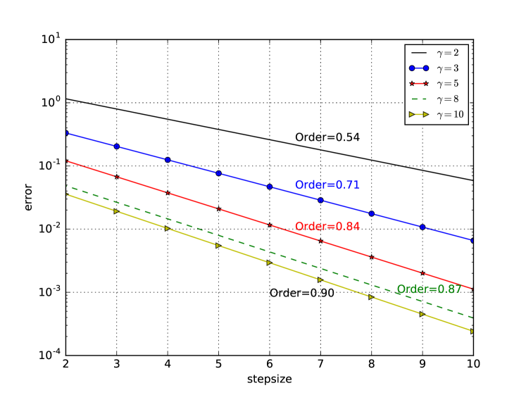
Figure 1. $L^{2}$ convergence of the randomized Riemann sum to Eqn. (40)

According to Theorem 3.1, the convergence order depends on the integrability of the function $g$. In Figure 1, the root-mean-squared errors were plotted versus the 2-logarithm of the underlying step size, i.e., the number $n$ on the x-axis indicates the step size $h=2^{-n}$. When $\gamma=0.5$, the observed order of convergence is as expected around $\frac{1}{2}$, since $g$ is only $L^{2-\epsilon}$ integrable. When increasing the value for $\gamma$ from $2$ to $10$, the regularity of $g$ is raised, which in turn gives an increase in the observed order of convergence from $0.54$ to $0.90$.

6.2. $L^{2}$ convergence for an ODE with jumps

Consider the following ODE with a non-continuous coefficient function:

(41) $$\begin{split}\begin{cases}\dot{u}(t)&=g(t)u,\quad t\in[0,T],\\ u(0)&=1,\end{cases}\end{split}$$

where $g(t):=\left[-\frac{1}{10}\mbox{sgn}(\frac{1}{4}T-t)-\frac{1}{5}\mbox{sgn}(\frac{1}{2}T-t)-\frac{7}{10}\mbox{sgn}(\frac{3}{4}T-t)\right]$ and

(42) $$\mbox{sgn}(t):=\begin{split}\begin{cases}-1,&\ \mbox{if\ }t<0,\\ 0,&\ \mbox{if\ }t=0,\\ 1,&\ \mbox{if\ }t>0.\end{cases}\end{split}$$

Here we have three jump points at $t=\frac{1}{4}T$, $t=\frac{1}{2}T$ and $t=\frac{3}{4}T$. It is easy to see that the exact solution at terminal time equals $\exp(-\frac{3}{10}T)$. We perform the numerical experiment with the classical Euler scheme, the randomized Euler scheme (3) and the randomized Runge-Kutta scheme (4), respectively. A comparison of the $L^{2}$-errors at the final time $T=1$ is shown in Figure 2, where the errors have been approximated by a Monte Carlo simulation with $1000$ independent samples for the same step sizes as in Section 6.1.

Figure 2. $L^{2}$-errors versus step sizes for Eqn. (41)

Note that by our choice of the step sizes the classical Euler scheme always evaluates the mapping $g$ at the three jump points. But due to the definition of the sign function, one of the summands in the definition of $g$ is always equal to zero at the jump points, causing $g$ to be neither left continuous nor right continuous at these points. For instance, we have $g(\frac{1}{2})=-\frac{3}{5}$, while $g(\frac{1}{2}+\epsilon)=-\frac{2}{5}$ and $g(\frac{1}{2}-\epsilon)=-\frac{4}{5}$ for all $\epsilon\in(0,\frac{1}{4})$. This causes an additional error of order $h$ in each step of the classical Euler scheme, where a jump point of $g$ is involved.

On the other hand, this type of error is avoided by both randomized numerical methods, since the random variable $\tau$ will prevent the evaluation of $g$ at jump points almost surely. This explains why both randomized methods perform better than the classical method if we compare the $L^{2}$-errors for the same step sizes. Further, although the coefficient function $g$ is not continuous with respect to the time variable, we observe an experimental convergence of order $1.51$ for the randomized Runge-Kutta method (4). This is well in agreement with the maximum order of convergence that has been proven for that method in Theorem 5.2.

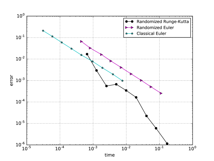
Figure 3. CPU time versus $L^{2}$ errors

Next, let us briefly compare the computational efficiency of the three methods under consideration. By also taking the necessity of drawing a random number at each step into consideration, the two randomized Runge-Kutta methods (3) and (4) are of course computationally more expensive than the classical Euler method. For this reason we compare in Figure 3 the average CPU times of these three schemes versus their accuracy. From this figure we can see that the classical Euler method is as expected the fastest method and, since it still converges with the same experimental order as the randomized Euler method (3), it is in total more efficient than its randomized counter-part. On the other hand, the computationally even more expensive randomized Runge-Kutta method (4) quickly offsets its higher cost with its higher order of convergence.

References

• [1] H. Bauer. Measure and integration theory, volume 26 of de Gruyter Studies in Mathematics. Walter de Gruyter & Co., Berlin, 2001. Translated from the German by Robert B. Burckel.
• [2] D. L. Burkholder. Martingale transforms. Ann. Math. Statist., 37:1494–1504, 1966.
• [3] J. C. Butcher. On Runge-Kutta processes of high order. J. Austral. Math. Soc., 4:179–194, 1964.
• [4] J. C. Butcher. Numerical Methods for Ordinary Differential Equations. John Wiley & Sons, Ltd., Chichester, second edition, 2008.
• [5] D. L. Cohn. Measure theory. Birkhäuser Advanced Texts: Basler Lehrbücher. Birkhäuser/Springer, New York, second edition, 2013.
• [6] I. Coulibaly and C. Lécot. A quasi-randomized Runge-Kutta method. Math. Comp., 68(226):651–659, 1999.
• [7] T. Daun. On the randomized solution of initial value problems. J. Complexity, 27(3-4):300–311, 2011.
• [8] T. Daun and S. Heinrich. Complexity of parametric initial value problems in Banach spaces. J. Complexity, 30(4):392–429, 2014.
• [9] E. Emmrich. Discrete versions of Gronwall’s lemma and their application to the numerical analysis of parabolic problems. TU Berlin, Fachbereich Mathematik, Preprint, 637-1999, 1999.
• [10] M. Evans and T. Swartz. Approximating integrals via Monte Carlo and deterministic methods. Oxford Statistical Science Series. Oxford University Press, Oxford, 2000.
• [11] P. K. Friz and M. Hairer. A Course on Rough Paths. Universitext. Springer, Cham, 2014. With an introduction to regularity structures.
• [12] R. D. Grigorieff. Numerik gewöhnlicher Differentialgleichungen, Band 1: Einschrittverfahren. B. G. Teubner, Stuttgart, 1972.
• [13] I. Gyöngy. A note on Euler’s approximations. Potential Anal., 8(3):205–216, 1998.
• [14] S. Haber. A modified Monte-Carlo quadrature. Math. Comp., 20:361–368, 1966.
• [15] S. Haber. A modified Monte-Carlo quadrature. II. Math. Comp., 21:388–397, 1967.
• [16] E. Hairer, S. P. Nørsett, and G. Wanner. Solving ordinary differential equations. I, volume 8 of Springer Series in Computational Mathematics. Springer-Verlag, Berlin, second edition, 1993. Nonstiff problems.
• [17] J. K. Hale. Ordinary differential equations. Robert E. Krieger Publishing Co., Inc., Huntington, N.Y., second edition, 1980.
• [18] S. Heinrich. Complexity of initial value problems in Banach spaces. Zh. Mat. Fiz. Anal. Geom., 9(1):73–101, 116, 2013.
• [19] S. Heinrich and B. Milla. The randomized complexity of initial value problems. J. Complexity, 24(2):77–88, 2008.
• [20] A. Jentzen and A. Neuenkirch. A random Euler scheme for Carathéodory differential equations. J. Comput. Appl. Math., 224(1):346–359, 2009.
• [21] B. Kacewicz. Optimal solution of ordinary differential equations. J. Complexity, 3(4):451–465, 1987.
• [22] B. Kacewicz. Almost optimal solution of initial-value problems by randomized and quantum algorithms. J. Complexity, 22(5):676–690, 2006.
• [23] O. Kallenberg. Foundations of modern probability. Probability and its Applications (New York). Springer-Verlag, New York, second edition, 2002.
• [24] A. Klenke. Probability theory. Universitext. Springer, London, second edition, 2014. A comprehensive course.
• [25] P. E. Kloeden and A. Neuenkirch. The pathwise convergence of approximation schemes for stochastic differential equations. LMS J. Comput. Math., 10:235–253, 2007.
• [26] X. Mao. Stochastic differential equations and applications. Horwood Publishing Limited, Chichester, second edition, 2008.
• [27] T. Müller-Gronbach, E. Novak, and K. Ritter. Monte Carlo-Algorithmen. Springer-Lehrbuch. [Springer Textbook]. Springer, Heidelberg, 2012.
• [28] B. Øksendal. Stochastic differential equations. Universitext. Springer-Verlag, Berlin, sixth edition, 2003. An introduction with applications.
• [29] P. Przybyłowicz and P. Morkisz. Strong approximation of solutions of stochastic differential equations with time-irregular coefficients via randomized Euler algorithm. Appl. Numer. Math., 78:80–94, 2014.
• [30] G. Stengle. Numerical methods for systems with measurable coefficients. Appl. Math. Lett., 3(4):25–29, 1990.
• [31] G. Stengle. Error analysis of a randomized numerical method. Numer. Math., 70(1):119–128, 1995.