New Flexible Compact Covariance Model
on a Sphere

Abstract

We discuss how the kernel convolution approach can be used to accurately approximate the spatial covariance model on a sphere using spherical distances between points. A detailed derivation of the required formulas is provided. The proposed covariance model approximation can be used for non-stationary spatial prediction and simulation in the case when the dataset is large and the covariance model can be estimated separately in the data subsets.

I Introduction

To perform kriging on a sphere, one can use “great arc/circle” distance metrics (the shortest distance on the surface of a sphere) to compute distances between points and the covariance model which is positive definite on a sphere. Among the valid covariance models are spherical, stable with shape parameter $\displaystyle\alpha\leq 1$, and K-Bessel (same as Matern) with shape parameter $\displaystyle\alpha\leq\dfrac{1}{2}$, see, for example, [1]. Disadvantages of this approach include the following:

• The allowed covariance models are not flexible because they change rapidly at short distances.

• These covariance models are isotropic. However, the analysis of various data has shown that an assumption of isotropy is generally inappropriate for global data because most of the geographical data are not stationary in latitude [2].

• It is not necessarily true that the best model on the plane is also the best on the surface of a sphere and it seems important to derive new flexible covariance models which are valid on a sphere and correspond to particular physical processes.

A covariance model with zero values when the distance between two points exceeds specified threshold value has a compact support. Compactly supported covariance functions allow for computationally efficient sparse matrix techniques usage, which is especially important when dealing with large datasets. [3] provides comprehensive review on the compact covariance construction for both stationary and non-stationary models on the plane and develops non-stationary compactly supported covariance functions for the spherical family. One advantage of the spherical model is its closed-form expression. However, the model proposed in [3] is not flexible enough because it has a fixed shape. [4] shows how flexible compact covariance model can be approximated numerically for further efficient use in prediction and simulation. In this paper we propose flexible compact covariance model which describes both weak and strong spatial correlation on a sphere. If required, non-stationary model can be constructed as shown in the conclusion section below.

Some of the issues listed above can be resolved by using the kernel/convolution approach. Taking into account that the shortest distance on the unit sphere is the angle (in radians) between two locations on a plane passing through the sphere center and the two points, we define the following kernel function:

$${\operatorname{k}}\left(h|\mu,\nu\right)=\left\{\begin{aligned} &\left(1-h^{\mu}\right)^{\nu},\text{if }h<1,\\ &0,\text{otherwise},\end{aligned}\right.$$ (1)

where $\displaystyle\mu>0$ and $\displaystyle\nu>0$ are the shape parameters and $\displaystyle h\geq 0$ is the distance from the center of the kernel.

On a sphere, kernel $\displaystyle{\operatorname{k}}\left(h|\mu,\nu\right)$ can be represented as

$${\operatorname{k}}\left(s|s_{*},r,\mu,\nu\right)=\dfrac{{\operatorname{k}}\left(\left.\frac{2\cdot\operatorname{SphericalDistance}\left(s,s_{*}\right)}{r}\right|\mu,\nu\right)}{\sqrt{\oiint{k^{2}{\left(\left.\frac{2\cdot\operatorname{SphericalDistance}\left(s^{\prime},s_{*}\right)}{r}\right|\mu,\nu\right)}\cdot\operatorname{d\!}s^{\prime}}}},$$

where $\displaystyle s_{*}$ is the location of the kernel center on a sphere, $\displaystyle s$ is the location where kernel value is calculated, $\displaystyle\dfrac{r}{2}$ is radius of the kernel (in radians), $\displaystyle\operatorname{SphericalDistance}$ is the shortest distance on the surface of a sphere, see formula (3) in section II below. The integration ($\displaystyle\oiint$) is performed on the surface of a sphere.

Kernel (1) generates the following random process on a sphere:

$$Y\left(s\right)=\oiint{{\operatorname{k}}\left(s^{\prime}|s,r,\mu,\nu\right)\cdot\operatorname{d\!}{\operatorname{W}}\left(s^{\prime}\right)},$$

where $\displaystyle{\operatorname{W}}\left(s^{\prime}\right)$ is a diffusion process in three dimensions, $\displaystyle\operatorname{d\!}{\operatorname{W}}\left(s^{\prime}\right)$ is white noise, $\displaystyle{\operatorname{E}}\left[\oiint\limits_{A}{\operatorname{d\!}{\operatorname{W}}\left(s^{\prime}\right)}\right]=0$, and $\displaystyle{\operatorname{Var}}\left[\oiint\limits_{A}{\operatorname{d\!}{\operatorname{W}}\left(s^{\prime}\right)}\right]=$ $\displaystyle\oiint\limits_{A}{\operatorname{d\!}s^{\prime}}$ $\displaystyle\forall A$, where $\displaystyle A$ is some integrable area on a sphere.

The relationship between the kernel and the covariance function is the following:

$${\operatorname{Cov}}\left[Y\left(s_{1}\right),Y\left(s_{2}\right)\right]=\oiint{{\operatorname{k}}\left(s^{\prime}|s_{1},r,\mu,\nu\right)\cdot{\operatorname{k}}\left(s^{\prime}|s_{2},r,\mu,\nu\right)\cdot\operatorname{d\!}s^{\prime}}.$$

Note that a kernel with radius $\displaystyle\dfrac{r}{2}$ generates the covariance function with a range equal to $\displaystyle r$ and the covariance depends only on the angle $\displaystyle\alpha$ between points,

$${\operatorname{C}}\left(\alpha|r,\mu,\nu\right)=\oiint{{\operatorname{k}}\left(s^{\prime}|(1,0,0),r,\mu,\nu\right)\cdot{\operatorname{k}}\left(s^{\prime}|(\cos\left(\alpha\right),\sin\left(\alpha\right),0),r,\mu,\nu\right)\cdot\operatorname{d\!}s^{\prime}}.$$ (2)

The covariance shape is a function of the range and parameters $\displaystyle\mu$ and $\displaystyle\nu$ in contrast to the covariance defined on the plane, which is a function of the parameters $\displaystyle\mu$ and $\displaystyle\nu$ only. This feature of the covariance on a sphere is important for the calculations optimization.

Unfortunately, not all kernel functions are integrable. Moreover, numerical evaluation of the positive-definite property of the covariance is problematic because it should be done with high precision. In the case of approximate integration, there is no guarantee that the resulting covariance model is positive definite and that the model describes the same stochastic process as the model which is calculated exactly.

One recent attempt to find an approximate solution of the problem was made in [5]. The author of [5] assumes that the parameters of the random field at each latitude are homogeneous and the modeling process at each latitude is isotropic. The kernel was chosen in such a way that its convolution gives covariance with the shape similar to the Matern one (however, for simplicity, it was assumed that the shape parameter is fixed and constant on the entire globe). It was also assumed that the data are absolutely precise so that the nugget effect is zero. Another assumption was that the sill and range are constants at each latitude, but they are changing smoothly between the latitudes. Then the values of the sill and range were found in one dimension for a fixed number of latitudes and a linear smoother was used to interpolate these estimates. Finally, the convolution of kernels was found numerically using the sets of discrete values inside the predefined ranges of each kernel parameter and it was reported that the approximation error was less than $\displaystyle 0.01$.

However, the error of $\displaystyle 0.01$ is too large for calculation of the covariance model. Consider the Matern covariance with effective range of $\displaystyle 1$. The graph in Figure 1 shows the proportion of effective range at which calculation of the covariance is not possible due to the inaccuracy in the covariance matrix (when the determinant equals zero) as a function of the shape parameter. The error of $\displaystyle 0.01$ will lead to serious problem when the samples are separated by relatively small distances. For example, when the effective range is $\displaystyle 100$ km, the covariance values cannot be calculated for the distances between points less than $\displaystyle\approx\!\!6$ km for typical values of the shape parameter (in fact, these critical distances will be even larger because of numerical instability near the threshold at which the determinant equals zero). Therefore, the proposed approximation in [5] can be used only in a very special case when the error-free data are nearly regularly sampled and the effective range of the data correlation is $\displaystyle 10$ - $\displaystyle 20$ times larger than the distance between the neighboring samples.

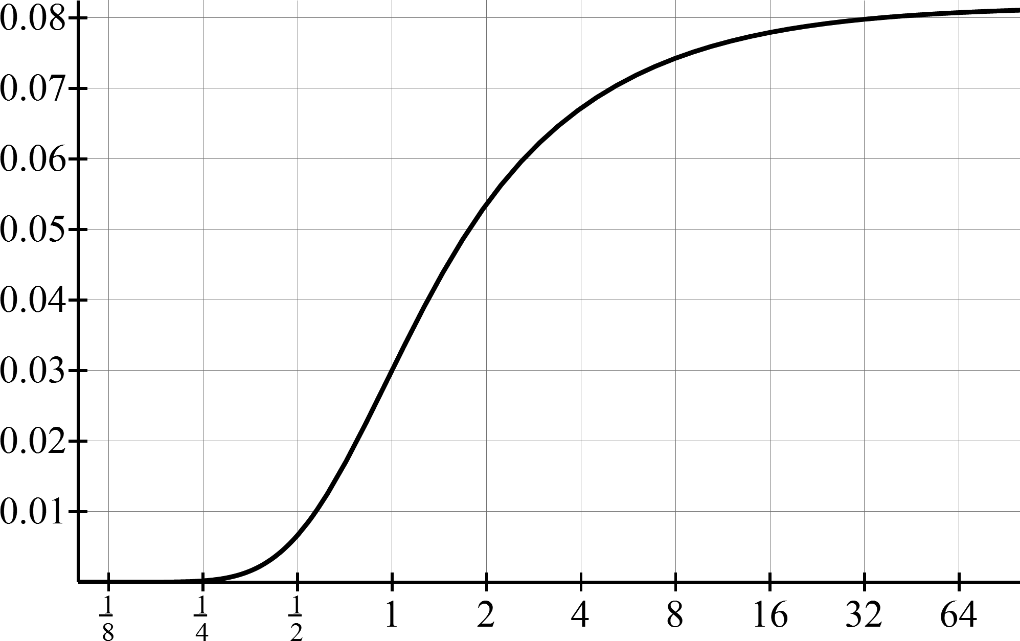
Figure 1: The proportion of effective range at which calculation of the covariance is not possible (axis Y) for the shape parameter of the Mattern covariance (axis X).

A model which overcomes most of the above-mentioned problems can be constructed based on the kernel-convolution approach proposed in [6] and [7]. In particular, [6] showed that the integral can be calculated analytically for any kernel step function on the plane. That methodology is also valid in larger dimensions.

Figure 2a shows the step functions for several kernels $\displaystyle{\operatorname{k}}\left(\cdot|\mu,\nu\right)$ defined in (1). The larger the number of steps, the more accurate the approximation of the kernel. Figure 2b shows a set of calculated flexible covariance models with the range of data correlation equal to $\displaystyle\pi$, the maximum distance between points on a sphere.

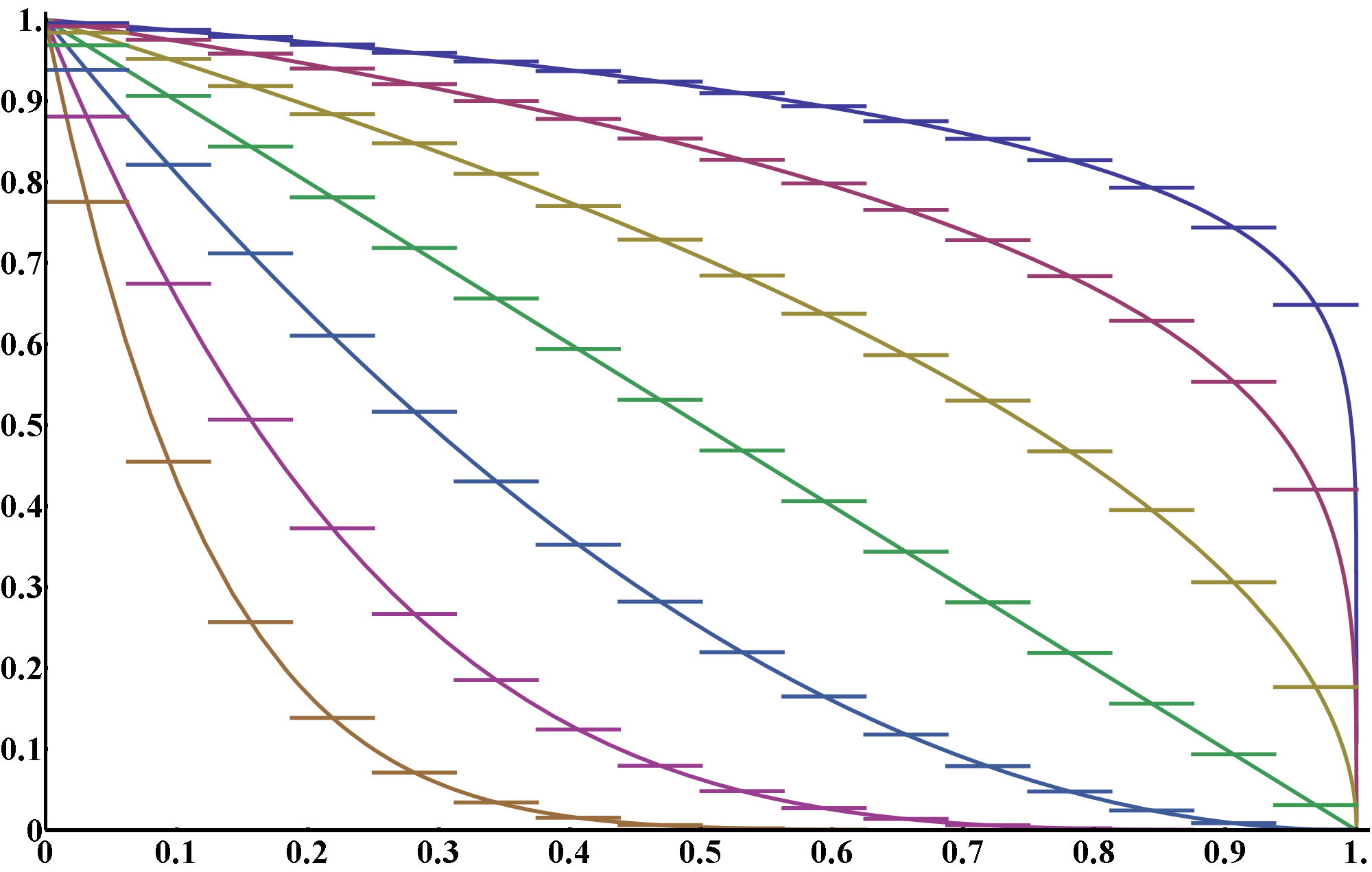
a)

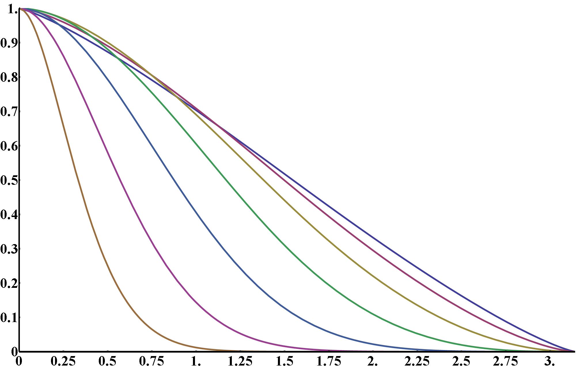
b)

Figure 2: Approximation of smooth kernel (1) by step function with $\displaystyle 16$ steps (a) and covariance function with range $\displaystyle\pi$ constructed by kernels with $\displaystyle 64$ steps (b) for $\displaystyle\mu=1$ and $\displaystyle\nu=\dfrac{1}{8}$, $\displaystyle\dfrac{1}{4}$, $\displaystyle\dfrac{1}{2}$, $\displaystyle 1$, $\displaystyle 2$, $\displaystyle 4$, and $\displaystyle 8$.

Numerically calculated covariance can be fitted using one of the available algorithms. We use restricted maximum likelihood, but other fitting algorithms, including weighted least squares, can be used as well.

In the next section, we show how the covariance can be produced by the kernel convolution with a kernel step function on a sphere. Formulas in the next section can be generalized to allow change of the kernel size and shape.

In the conclusion section, we discuss prediction and simulation with the proposed compactly supported covariance model on a sphere for both stationary and non-stationary data.

II Derivation of the covariance on a sphere produced by kernel convolution

In this section, we provide definitions and derivations required for calculation of the covariance on a unit sphere located at the origin of the coordinate system. Detailed information on the spherical geometry can be found, for example, in [8]. Note that all angles in the formulas below are in radians.

• A spherical segment is the shortest path connecting two points on the surface of a sphere. It coincides with the great arc passing through those two points.

• A spherical distance between points $\displaystyle\left(x_{1},y_{1},z_{1}\right)$ and $\displaystyle\left(x_{2},y_{2},z_{2}\right)$ on a sphere is

  $$\operatorname{SphericalDistance}{\left(\left(x_{1},y_{1},z_{1}\right),\left(x_{2},y_{2},z_{2}\right)\right)}=\arccos{\left(x_{1}\cdot x_{2}+y_{1}\cdot y_{2}+z_{1}\cdot z_{2}\right)}=\\ =2\arcsin{\left(\tfrac{\sqrt{\left(x_{2}-x_{1}\right)^{2}+\left(y_{2}-y_{1}\right)^{2}+\left(z_{2}-z_{1}\right)^{2}}}{2}\right)}.$$ (3)

  This distance equals the angle between two points on a sphere from its center. The formula based on $\displaystyle\arcsin$ has higher precision for small angles.

• A spherical triangle consists of spherical segments $\displaystyle AB$, $\displaystyle BC$, and $\displaystyle AC$, where $\displaystyle A$, $\displaystyle B$, and $\displaystyle C$ are points on a sphere.

• A spherical angle is an angle on the surface of a sphere between two spherical segments, see Figure 3. To distinguish spherical angles from plane angles, the symbol $\displaystyle\sphericalangle$ is used.

• A spherical right triangle is a spherical triangle where one spherical angle equals $\displaystyle\dfrac{\pi}{2}$ (right angle).

Figure 3: Spherical angle $\displaystyle\sphericalangle{ABC}$, shown as thick red arc, between two spherical segments $\displaystyle AB$ and $\displaystyle BC$.

Using the definitions above, several spherical geometry relationships between spherical segments and angles follows.

1. The relationship between sides $\displaystyle a$, $\displaystyle b$, and hypotenuse $\displaystyle c$ of spherical right triangle [8], see Figure 4, is:

   $$\cos{\left(c\right)}=\cos{\left(a\right)}\cdot\cos{\left(b\right)}.$$ (4)

   This is equivalent to

   $$\sin^{2}{\left(\dfrac{c}{2}\right)}=\sin^{2}{\left(\dfrac{a}{2}\right)}+\sin^{2}{\left(\dfrac{b}{2}\right)}-2\sin^{2}{\left(\dfrac{a}{2}\right)}\cdot\sin^{2}{\left(\dfrac{b}{2}\right)}$$ (5)

   (5) has better precision than (4) for small angles.

   This is equivalent to the Pythagorean theorem. Notice that (5) tends toward $\displaystyle c^{2}=a^{2}+b^{2}$, when $\displaystyle a$, $\displaystyle b$, and $\displaystyle c$ approach $\displaystyle 0$.

2. The relationship between spherical angle $\displaystyle\beta$, side $\displaystyle a$, and hypotenuse $\displaystyle c$ of spherical right triangle [8], see Figure 4, is:

   $$\cos{\left(\beta\right)}=\tan{\left(a\right)}\cdot\cot{\left(c\right)}.$$ (6)

   This is equivalent to the definition of cosine for right triangles. Notice that (6) tends toward $\displaystyle\cos\beta=\dfrac{a}{c}$, when $\displaystyle a$ and $\displaystyle c$ approach $\displaystyle 0$.

Figure 4: Spherical right triangle.

1. The area of a spherical right triangle with sides $\displaystyle a$ and $\displaystyle b$, see Figure 4 and [8], is:

   $$\operatorname{RightTriangleArea}{\left(a,b\right)}=2\arctan{\left(\tan{\left(\dfrac{a}{2}\right)}\cdot\tan{\left(\dfrac{b}{2}\right)}\right)}.$$ (7)

   Notice that (7) tends toward area of the right triangle $\displaystyle\dfrac{a\cdot b}{2}$, when $\displaystyle a$ and $\displaystyle b$ approach $\displaystyle 0$.

2. A spherical circle with radius $\displaystyle r$ at point $\displaystyle\left(x_{c},y_{c},z_{c}\right)$ is a set of points on the surface of a sphere with a spherical distance equal to $\displaystyle r$ from its center.

   A spherical disk with radius $\displaystyle r$ at point $\displaystyle\left(x_{c},y_{c},z_{c}\right)$ contains points on the surface of a sphere with a spherical distance less than or equal to $\displaystyle r$ from its center.

   A spherical ring is the area of the outer spherical disk excluding the inner spherical disk sharing the same center.

3. It follows that a maximum radius of a spherical disk is $\displaystyle\pi$. That spherical disk covers a sphere completely.

4. We ignore the edge of the spherical disk because it does not affect its area. The complement of a spherical disk with radius $\displaystyle r$ and center $\displaystyle\left(x_{c},y_{c},z_{c}\right)$ is a spherical disk with center at the opposite point on the surface of a sphere $\displaystyle\left(-x_{c},-y_{c},-z_{c}\right)$ with radius equal to $\displaystyle\pi-r$.

5. From (V) and (VI), it follows that a minimum radius of a spherical disk and its complement is less than or equal to $\displaystyle\dfrac{\pi}{2}$.

6. The area inside the spherical disk with radius $\displaystyle r$ is

   $$\operatorname{DiskArea}{\left(r\right)}=2\pi\cdot(1-\cos{\left(r\right)})=4\pi\cdot\sin^{2}{\left(\dfrac{r}{2}\right)}.$$ (8)

   The area of the spherical circular sector, defined in Figure 5, with sector spherical angle $\displaystyle\alpha$ and radius $\displaystyle r$ is

   $$\operatorname{CircularSectorArea}{\left(\alpha,r\right)}=\alpha\cdot(1-\cos{\left(r\right)})=2\alpha\cdot\sin^{2}{\left(\dfrac{r}{2}\right)}.$$

Figure 5: Spherical circular sector (see definition of planar circular sector in [9]) with spherical circular segment (see definition of planar circular segment in [10]) area in red.

1. From (V) and (8), the area of a sphere is $\displaystyle 4\pi$.

2. The area of the spherical circular segment, see Figure 5, is

   $$\operatorname{CircularSegmentArea}{\left(\alpha,r,a,b\right)}=2\left(\operatorname{CircularSectorArea}{\left(\alpha,r\right)}-\operatorname{RightTriangleArea}{\left(a,b\right)}\right).$$

Now we have all necessary formulas for the covariance calculations. First, we define the kernel step function as

$${\operatorname{k}}\left(h\right)=\sum\limits_{j=1}^{n}{\left(a_{j}\cdot\delta_{r_{j-1}\leq h\wedge h<r_{j}}\right)}=\sum\limits_{j=1}^{n}{\left(b_{j}\cdot\delta_{h<r_{j}}\right)},$$ (9)

where $\displaystyle n$ is the number of steps in the kernel function, $\displaystyle a_{j}$ is the value of the kernel function at step $\displaystyle j$, $\displaystyle j=\overline{1..n}$, $\displaystyle b_{j}=a_{j}-a_{j+1}$, $\displaystyle j=\overline{1..n-1}$ and $\displaystyle b_{n}=a_{n}$, $\displaystyle r_{j}$ is a sequence of steps, $\displaystyle j=\overline{0..n}$ ($\displaystyle 0=r_{0}<r_{1}<r_{2}<...<r_{n}\leq\pi$), $\displaystyle\delta_{\theta}$ is $\displaystyle 1$ when $\displaystyle\theta$ is true and $\displaystyle 0$ otherwise.

The kernel step function located at point $\displaystyle\left(x_{c},y_{c},z_{c}\right)$ is

$${\operatorname{k}}\left(\left(x,y,z\right)|\left(x_{c},y_{c},z_{c}\right)\right)={\operatorname{k}}\left(\operatorname{SphericalDistance}\left(\left(x,y,z\right),\left(x_{c},y_{c},z_{c}\right)\right)\right).$$

Figure 6 shows four different kernels on a sphere.

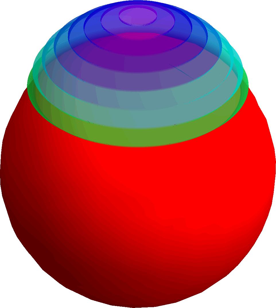
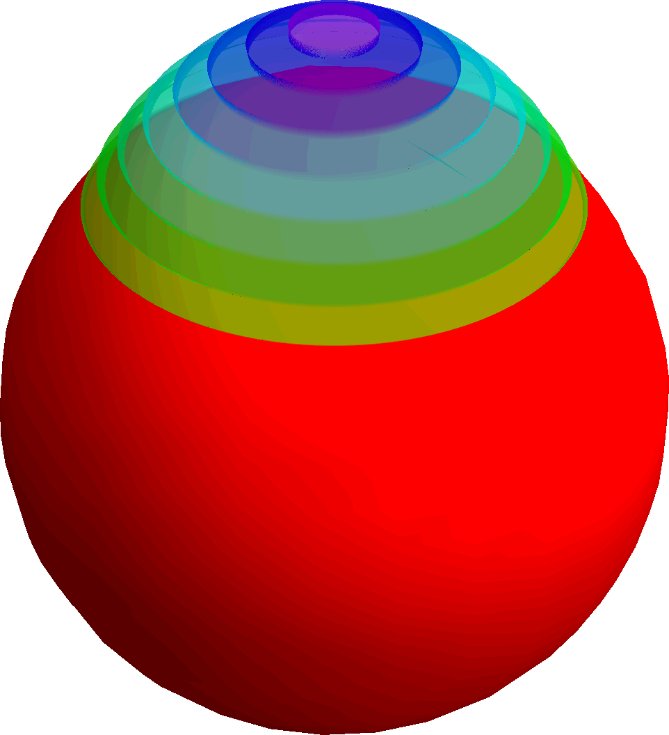
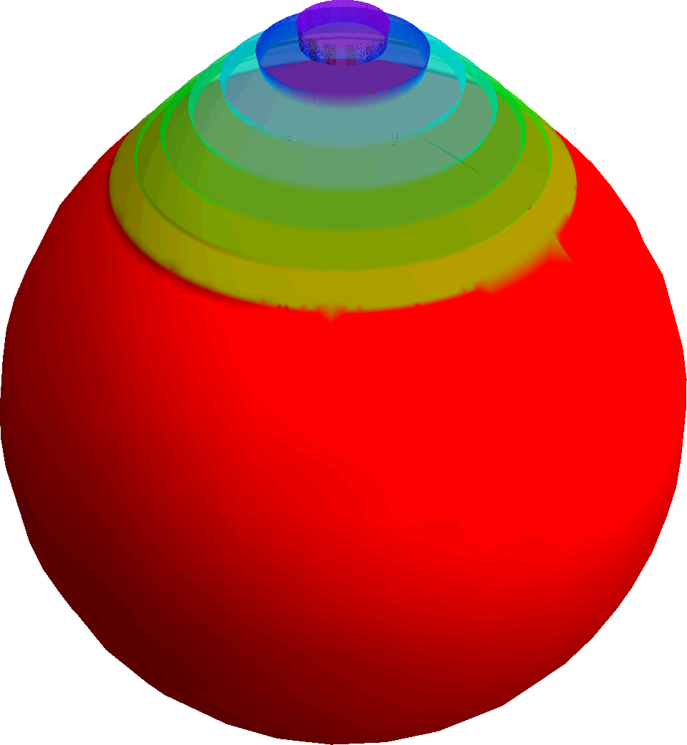
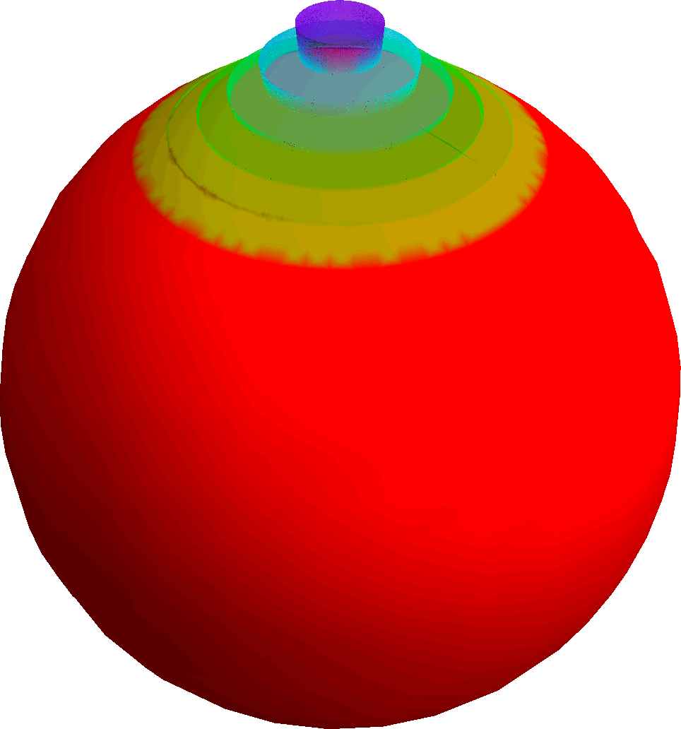
Figure 6: Four kernel step functions located at the top of a sphere.

To construct the covariance function with variance equal to $\displaystyle 1$, the kernel function at any location $\displaystyle\left(x_{c},y_{c},z_{c}\right)$ must satisfy the following constraint:

$$\oiint{{\operatorname{k}^{2}}\left(\left(x,y,z\right)|\left(x_{c},y_{c},z_{c}\right)\right)\cdot\operatorname{d\!}s}=1.$$ (10)

Equation (10) can be rewritten as

$$\oiint{{\operatorname{k}^{2}}\left(\left(x,y,z\right)|\left(x_{c},y_{c},z_{c}\right)\right)\cdot\operatorname{d\!}s}=\oiint{{\operatorname{k}^{2}}\left(\operatorname{SphericalDistance}\left(\left(x,y,z\right),\left(x_{c},y_{c},z_{c}\right)\right)\right)\cdot\operatorname{d\!}s}=\\ =\sum\limits_{k=1}^{n}{\left(a_{k}^{2}\cdot\left(\operatorname{DiskArea}{\left(r_{k}\right)}-\operatorname{DiskArea}{\left(r_{k-1}\right)}\right)\right)}=1.$$

To satisfy (10), the coefficient $\displaystyle a_{j}$ in (9) is replaced with

$$\dfrac{a_{j}}{\sqrt{\sum\limits_{k=1}^{n}{\left(a_{k}^{2}\cdot\left(\operatorname{DiskArea}{\left(r_{k}\right)}-\operatorname{DiskArea}{\left(r_{k-1}\right)}\right)\right)}}}$$

Next step in the kernel convolution construction is calculation of the intersection area of spherical disks, for example, green and blue spherical disks in Figure 7.

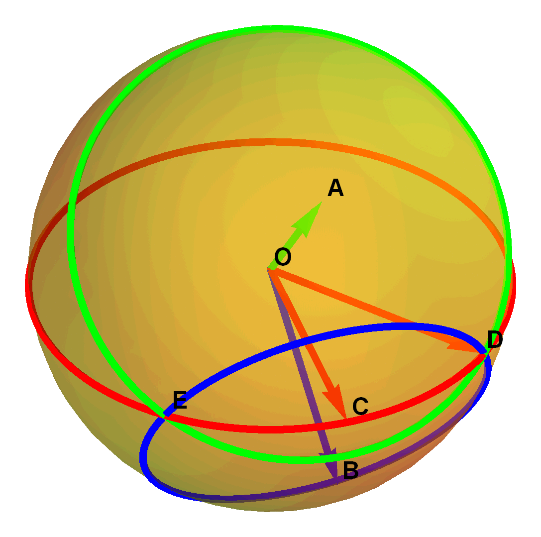
Figure 7: Intersection of the green spherical circle with center $\displaystyle A$ and radius $\displaystyle r_{0}=\angle{AOD}$ and the blue spherical circle with center $\displaystyle B$ and radius $\displaystyle r_{1}=\angle{BOD}$. Spherical distance between $\displaystyle A$ and $\displaystyle B$ equals $\displaystyle d$. These spherical circles intersect at points $\displaystyle D$ and $\displaystyle E$. $\displaystyle DE$ is a spherical segment. Point $\displaystyle C$ is between $\displaystyle E$ and $\displaystyle D$. $\displaystyle O$ is the center of a sphere.

If a spherical disk is larger than $\displaystyle\dfrac{\pi}{2}$, its complement will be used instead (see (VI) and (VII)).

When $\displaystyle r_{0}>\dfrac{\pi}{2}$,

$$\operatorname{IntersectionArea}{\left(r_{0},r_{1},d\right)}=\operatorname{DiskArea}{\left(r_{1}\right)}-\operatorname{IntersectionArea}{\left(\pi-r_{0},r_{1},\pi-d\right)}.$$ (11)

When $\displaystyle r_{1}>\dfrac{\pi}{2}$,

$$\operatorname{IntersectionArea}{\left(r_{0},r_{1},d\right)}=\operatorname{DiskArea}{\left(r_{0}\right)}-\operatorname{IntersectionArea}{\left(r_{0},\pi-r_{1},\pi-d\right)}.$$ (12)

If both spherical radii are larger than $\displaystyle\dfrac{\pi}{2}$, then, from (11), (12), and (IX),

$$\operatorname{IntersectionArea}{\left(r_{0},r_{1},d\right)}=\operatorname{DiskArea}{\left(r_{0}\right)}+\operatorname{DiskArea}{\left(r_{1}\right)}-4\pi+\operatorname{IntersectionArea}{\left(\pi-r_{0},\pi-r_{1},d\right)}.$$

Therefore, it is sufficient to calculate the intersection area for spherical disks with radii less than or equal to $\displaystyle\dfrac{\pi}{2}$.

If $\displaystyle r_{0}+r_{1}\leq d$, then the intersection area is equal to zero. If $\displaystyle r_{1}\leq r_{0}-d$, then the blue spherical disk in Figure 7 is inside the green spherical disk and the intersection area is equal to the area of the blue spherical disk. If $\displaystyle r_{0}\leq r_{1}-d$, then the green spherical disk is inside the blue spherical disk and the intersection area is equal to the area of the green spherical disk. Otherwise, they intersect each other. In that last case, we need to find the following angles: $\displaystyle\angle{AOC}$, $\displaystyle\angle{BOC}$, $\displaystyle\angle{COD}$, $\displaystyle\sphericalangle{CAD}$, $\displaystyle\sphericalangle{CBD}$, $\displaystyle\sphericalangle{ADC}$, and $\displaystyle\sphericalangle{BDC}$. These angles are calculated as follows:

$$\angle{AOC}= \left.\dfrac{d}{2}+x\right., \angle{BOC}= \left.\dfrac{d}{2}-x\right.,$$

where

$$x=\arctan{\left(\cot{\left(\frac{d}{2}\right)}\cdot\dfrac{\sin^{2}{\left(\frac{r_{0}}{2}\right)}-\sin^{2}{\left(\frac{r_{1}}{2}\right)}}{1-\left(\sin^{2}{\left(\frac{r_{0}}{2}\right)}+\sin^{2}{\left(\frac{r_{1}}{2}\right)}\right)}\right)}.$$ (13)

Because $\displaystyle r_{0}$ and $\displaystyle r_{1}$ can be close to $\displaystyle\dfrac{\pi}{2}$, care has to be taken when evaluating $\displaystyle\dfrac{\sin^{2}{\left(\dfrac{r_{0}}{2}\right)}-\sin^{2}{\left(\dfrac{r_{1}}{2}\right)}}{1-\left(\sin^{2}{\left(\dfrac{r_{0}}{2}\right)}+\sin^{2}{\left(\dfrac{r_{1}}{2}\right)}\right)}$. When both radii equals $\displaystyle\dfrac{\pi}{2}$, any value between $\displaystyle-1$ and $\displaystyle 1$ can be used.

This is equivalent to the problem of finding the intersection of disks on the plane. Notice that (13) tends toward $\displaystyle x=\dfrac{r_{0}^{2}-r_{1}^{2}}{2d},$ when $\displaystyle r_{0}$, $\displaystyle r_{1}$, and $\displaystyle d$ approach $\displaystyle 0$.

Since $\displaystyle\sphericalangle{ACD}$, $\displaystyle\sphericalangle{ACE}$, $\displaystyle\sphericalangle{BCD}$, and $\displaystyle\sphericalangle{BCE}$ are spherical right angles, it follows from (I) that $\displaystyle\angle{COD}$ can be calculated using one of the following formulas:

$$\angle{COD}=2\arcsin{\sqrt{\dfrac{\sin^{2}{\left(\dfrac{r_{0}}{2}\right)}-\sin^{2}{\left(\dfrac{\angle{AOC}}{2}\right)}}{1-2\sin^{2}{\left(\dfrac{\angle{AOC}}{2}\right)}}}}\text{ or }\angle{COD}=2\arcsin{\sqrt{\dfrac{\sin^{2}{\left(\dfrac{r_{1}}{2}\right)}-\sin^{2}{\left(\dfrac{\angle{BOC}}{2}\right)}}{1-2\sin^{2}{\left(\dfrac{\angle{BOC}}{2}\right)}}}}.$$

In the formulas above, the denominator under the square root can be close to zero. Therefore, to avoid numerical instability, the equation with the largest denominator should be used. Note that $\displaystyle\angle{COD}$ is always less than or equal to the minimum of $\displaystyle r_{0}$ and $\displaystyle r_{1}$.

Using expression (II), $\displaystyle\sphericalangle{CAD}$ and $\displaystyle\sphericalangle{CBD}$ can be calculated as

$$\sphericalangle{CAD}= \arccos{\left(\cot{\left(r_{0}\right)}\cdot\tan{\left(\angle{AOC}\right)}\right)},$$

$$\sphericalangle{CBD}= \arccos{\left(\cot{\left(r_{1}\right)}\cdot\tan{\left(\angle{BOC}\right)}\right)}.$$

Next, the intersection area of spherical disks is calculated using (X) as

$$\operatorname{IntersectionArea}{\left(r_{0},r_{1},d\right)}=\\ =\operatorname{CircularSegmentArea}{\left(\sphericalangle{CAD},r_{0},\angle{COD},\angle{AOC}\right)}+\operatorname{CircularSegmentArea}{\left(\sphericalangle{CBD},r_{1},\angle{COD},\angle{BOC}\right)}.$$ (14)

There are two cases when centers of the spherical circles $\displaystyle A$ and $\displaystyle B$ are located on both sides of $\displaystyle ECD$ and when $\displaystyle A$ and $\displaystyle B$ are on the same side. Formula (14) is correct for both cases. Note that in the case when both centers of the spherical circles $\displaystyle A$ and $\displaystyle B$ are located on the same side of $\displaystyle ECD$, the sign of the area of one of the spherical triangles is negative.

In anisotropic case, to avoid solving a problem of finding intersection of two ellipses on a sphere, the ellipses can be approximated using four spherical arcs as described in [11].

Finally, the covariance between two locations separated by the spherical distance $\displaystyle d$ is produced by convolution of two kernels. Using (9) and (14), the covariance between locations $\displaystyle\left(x_{1},y_{1},z_{1}\right)$ and $\displaystyle\left(x_{2},y_{2},z_{2}\right)$ on a sphere, with spherical distance between points $\displaystyle\left(x_{1},y_{1},z_{1}\right)$ and $\displaystyle\left(x_{2},y_{2},z_{2}\right)$ equal to $\displaystyle d$, is

$${\operatorname{C}}\left(d\right)=\oiint{{\operatorname{k}}\left(\left(x,y,z\right)|\left(x_{1},y_{1},z_{1}\right)\right)\cdot{\operatorname{k}}\left(\left(x,y,z\right)|\left(x_{2},y_{2},z_{2}\right)\right)\cdot\operatorname{d\!}s}=\sum\limits_{j_{1}=1}^{n}{\sum\limits_{j_{2}=1}^{n}{\left(b_{j_{1}}\cdot b_{j_{2}}\cdot\operatorname{IntersectionArea}{\left(r_{j_{1}},r_{j_{2}},d\right)}\right)}}=$$

$$=\sum\limits_{j=1}^{n}{\left(b_{j}^{2}\cdot\operatorname{IntersectionArea}{\left(r_{j},r_{j},d\right)}\right)}+2\cdot\sum\limits_{j_{1}=1}^{n}{\sum\limits_{j_{2}=1}^{j_{1}-1}{\left(b_{j_{1}}\cdot b_{j_{2}}\cdot\operatorname{IntersectionArea}{\left(r_{j_{1}},r_{j_{2}},d\right)}\right)}}.$$

III Conclusion

One way to construct a valid covariance model in n/̄dimensional space is by performing kernel/convolution proposed in [6] and [7]. However, that methodology is not applicable for the data collected on a sphere because there is no regular grid with sufficient number of nodes for applying the fast Fourier transform algorithm as in [12]. Therefore, we define a kernel function as a set of rings and use these rings instead of rectangles as in [6] and [7]. For each ring, the kernel function has constant value. Our methodology extends the applicability of the kernel/convolution approach from n/̄dimensional space to the n/̄dimensional sphere.

When the kernel function is represented by a series of rectangles, the resultant covariance function is piece-wise bilinear and anisotropic. On the other hand, when the kernel function is constructed using rings, the resultant covariance function is isotropic, which allows for precalculation of the covariance model for further efficient use for the data fitting, predictions, and simulations.

The algorithm for prediction and simulation with compactly supported covariance on a sphere proposed in this paper can be the following:

1. Choose a set of kernels with fixed bandwidth.

2. Approximate these kernels using a step function.

3. Approximate the corresponding covariance model by piecewise polynomials and save the tabulated values of the covariance.

4. For prediction, fit the tabulated covariance, then find the corresponding kernel and perform kernel/convolutions kriging or use the covariance models merging as in [13].

5. For simulations, approximate kernels at the required locations as in [4], generate unconditional simulation using, for example, the approach from [14], and produce conditional simulation using the relationship between the kernels and covariance functions (2).

In practice, spatial data variation is changing from place to place and, in the case of interpolation of large datasets, it is advantageous to divide the data into subset, estimate the covariance model in that subsets and then use one of the available approaches for merging the models, as discussed, for example, in [13] for predictions and in [4] for simulations.

References

- [1] J. Guinness and M. Fuentes, “Covariance functions for mean square differentiable processes on spheres,” August 2013, (preprint). [Online]. Available: http://www.stat.ncsu.edu/information/library/papers/mimeo2652_Guinness.pdf
- [2] M. Hitczenko and M. L. Stein, “Some theory for anisotropic processes on the sphere,” Statistical Methodology, vol. 9, no. 1-2, pp. 211–227, 2012, special Issue on Astrostatistics + Special Issue on Spatial Statistics.
- [3] M. Liang and D. Marcotte, “A class of non-stationary covariance functions with compact support,” Stochastic Environmental Research and Risk Assessment, vol. 30, no. 3, pp. 973–987, 2015.
- [4] A. Gribov and K. Krivoruchko, “Simulations from spatially varying kriging model with compactly supported covariance,” in Proceedings of IAMG 2015, The 17th Annual Conference of the International Association for Mathematical Geosciences, H. Schaeben, R. T. Delgado, K. G. van den Boogaart, and R. van den Boogaart, Eds., Freiberg, Germany, September 2015, pp. 633–639, (DVD).
- [5] Y. Li, “Non-parametric and semi-parametric estimation of spatial covariance function,” Graduate Theses and Dissertations, p. 100, 2013, paper 13268. [Online]. Available: http://lib.dr.iastate.edu/etd/13268
- [6] R. P. Barry and J. M. Ver Hoef, “Blackbox kriging: Spatial prediction without specifying variogram models,” Journal of Agricultural, Biological, and Environmental Statistics, vol. 1, no. 3, pp. 297–322, September 1996. [Online]. Available: http://www.jstor.org/stable/1400521
- [7] D. Higdon, “A process-convolution approach to modelling temperatures in the north atlantic ocean,” Environmental and Ecological Statistics, vol. 5, no. 2, pp. 173–190, 1998.
- [8] I. Todhunter, Spherical Trigonometry, 5th ed. Project Gutenberg, November 2006. [Online]. Available: http://www.gutenberg.org/ebooks/19770
- [9] E. W. Weisstein, “Circular sector. From MathWorld–A Wolfram Web Resource.” [Online]. Available: http://mathworld.wolfram.com/CircularSector.html
- [10] ——, “Circular segment. From MathWorld–A Wolfram Web Resource.” [Online]. Available: http://mathworld.wolfram.com/CircularSegment.html
- [11] P. L. Rosin, “A survey and comparison of traditional piecewise circular approximations to the ellipse,” Computer Aided Geometric Design, vol. 16, no. 4, pp. 269–286, 1999.
- [12] J. M. Ver Hoef, N. Cressie, and R. P. Barry, “Flexible spatial models for kriging and cokriging using moving averages and the fast Fourier transform (FFT),” Journal of Computational and Graphical Statistics, vol. 13, no. 2, pp. 265–282, 2004. [Online]. Available: http://www.jstor.org/stable/1391176
- [13] K. Krivoruchko and A. Gribov, “Pragmatic Bayesian kriging for non-stationary and moderately non-gaussian data,” in Mathematics of Planet Earth, ser. Lecture Notes in Earth System Sciences, E. Pardo-Igúzquiza, C. Guardiola-Albert, J. Heredia, L. Moreno-Merino, J. J. Durán, and J. A. Vargas-Guzmán, Eds. Springer Berlin Heidelberg, 2014, pp. 61–64.
- [14] L. V. Hansen, T. L. Thorarinsdottir, E. Ovcharov, T. Gneiting, and D. Richards, “Gaussian random particles with flexible Hausdorff dimension,” ArXiv e-prints, February 2015. [Online]. Available: http://arxiv.org/abs/1502.01750