An epicycle method for elasticity limit calculations

Abstract

The task of finding the smallest energy needed to bring a solid to its onset of mechanical instability arises in many problems in materials science, from the determination of the elasticity limit to the consistent assignment of free energies to mechanically unstable phases. However, unless the space of possible deformations is low-dimensional and a priori known, this problem is numerically difficult, as it involves minimizing a function under a constraint on its Hessian, which is computionally prohibitive to obtain in low symmetry systems, especially if electronic structure calculations are used. We propose a method that is inspired by the well-known dimer method for saddle point searches but that adds the necessary ingredients to solve for the lowest onset of mechanical instability. The method consists of two nested optimization problems. The inner one involves a dimer-like construction to find the direction of smallest curvature as well as the gradient of this curvature function. The outer optimization then minimizes energy using the result of the inner optimization problem to constrain the search to the hypersurface enclosing all points of zero minimum curvature. Example applications to both model systems and electronic structure calculations are given.

I Introduction

The task of identifying a solid’s onset of mechanical instability Grimvall et al. (2012); Luo et al. (2002) arises in many problems in materials science and condensed matter physics, from the determination of the failure mechanisms Marianetti and Yevick (2010) to the consistent assignment of free energies to mechanically unstable phases van de Walle et al. (2015).

A complex feature of this problem is that the instability can occur along any phonon mode and not only along the direction of the applied stress or force. However, the task of computing the Hessian of the energy surface (i.e. performing a lattice dynamics calculation) at each level of applied strain and/or displacements can be computationally demanding. This is especially the case when electronic structure calculations are used, when the solid considered has a large unit cell or when a disordered alloy is considered. We propose a method to determine the point of mechanical instability that is inspired by the well-known dimer method Henkelman and Jonsson (1999); Voter (1997) for saddle point searches but that differs in two respect. First, we propose a slight modification of the dimer method, which we call the epicycle method, that provides roughly a factor two improvement in computational efficiency for the problem of determining the softest phonon mode. Second, we embed this epicycle into an outer-level optimization algorithm that searches for the lowest energy point that lies at the onset of mechanical instability.

Examples of applications to both model systems and electronic structure calculations are given. We consider the interesting case of the failure mechanism of graphene under tension Marianetti and Yevick (2010). We also devote special attention to the calculation of (free) energies of mechanically unstable phases van de Walle et al. (2015) and exploit the accuracy of the proposed method to analyze in detail how the calculated quantities vary smoothly with composition even through the onset of mechanical instability. We also demonstrate that different alloy systems which share a common element yield mutually consistent free energies for that element.

II Method

II.1 Numerical Method

II.1.1 Outline and notation

In a system of $N$ atoms, let $x$ denote the $3N$ vector of all atomic positions (and unit cell parameter, if the system is periodic), let $V(x)$ denote the potential energy of the system in that state and let $\kappa(x)$ be the minimum curvature at $x$, that is, the minimum eigenvalue of the Hessian (the matrix of second derivatives). Hence, $\kappa(x)>0$ and $\kappa(x)\leq 0$ correspond to mechanically stable and unstable regions, respectively. The goal is to numerically minimize the potential energy $V\left(x\right)$ with respect to $x$, subject to the constraint $\kappa\left(x\right)=0$. The key idea is that the constraint $\kappa(x)=0$ can be maintained by constraining the system to move perpendicular to direction along which $\kappa(x)$ varies the fastest. This follows from the fact that the normal to the hypersurface $\kappa(x)=0$ at $x$ is simply given by the gradient of $\kappa(x)$. However, it is desirable to avoid the need to compute the derivative of $\kappa\left(x\right)$, which is a third derivative of $V(x)$. In fact, we avoid the need to compute second derivatives as well, via a modification of the dimer method Henkelman and Jonsson (1999). In what follows, we let $|v|$ denote the Euclidian norm of a vector $v$ and subscripts denote partial derivatives.

II.1.2 Inner optimization problem

The goal of the inner optimization problem is to find $\kappa(x)$, the minimum curvature of $V(x)$ at $x$ and can be implemented as follows (refer to Figure 1). First, compute the gradient at $x$ and set $g_{0}=V_{x}(x)$. Next, determine the direction $u$ of minimum curvature by minimizing

$$V(x+u)-g_{0}\cdot u$$

over all $u$ such that $|u|=\epsilon$, where $\epsilon$ is a user-specified finite difference step. This procedure works by eliminating the linear term of Taylor expansion of $V(x)$ through the term $-g_{0}\cdot u$, so that the remaining quadratic form (up to a $\epsilon^{3}$ error) can be minimized over a hypersphere to find the direction of minimum curvature. For efficiency reasons, this minimization is implemented using the gradient of the objective function, which is equal to $V_{x}(x+u)-g_{0}$. This gradient, projected orthogonally to $u$, can be used to drive a conjugate gradient optimization algorithm Fletcher and Reeves (1964).

While this step could have been done in the same way as in the original dimer method Henkelman and Jonsson (1999); Voter (1997), we chose here to place the two images at $x$ and $x+u$ instead of at $x+u$ and $x-u$. The advantage is that the point $x$ does not move as $u$ is updated, so we only need to recompute one image at each optimization step, thus essentially halving the computational requirements. The disadvantage is that a non-central difference provides a lower order of accuracy. The latter effect can be mitigated at slight additional cost, by using a central difference only at the last step (or the last few steps). In this work, we use a central difference to compute the minimum curvature after the direction $u$ has been optimized with an non-central difference.

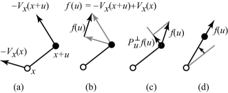
Figure 1: Epicycle algorithm for the determination of the direction of the most unstable phonon mode (inner optimization problem). The given structure is specified via the (fixed) vector $x$ while the direction of the mode will be determined by the vector $u$ to be optimized. (a) One first calculates the forces $-V_{x}\left(x\right)$, $-V_{x}\left(x+u\right)$ at points $x$ and $x+u$, respectively (the force $-V_{x}\left(x\right)\equiv-g_{0}$ needs to be calculated only once). Next, the difference $f\left(u\right)\equiv-V_{x}\left(x+u\right)+V_{x}\left(x\right)$ is calculated (b) and projected (c) orthogonal to $u$. This orthogonal force $P_{u}^{\perp}f\left(u\right)$ drives the optimization of the direction $u$, which continues until (d) the force $f\left(u\right)$ is parallel to $u$.

II.1.3 Outer optimization problem

This optimization problem seeks to minimize energy $V(x)$ under the constraint of $\kappa(x)=0$ and can be performed as follows (refer to Figure 2). This task will require the knowledge of the gradient of $\kappa(x)$, denoted $\kappa_{x}(x)$. To find a convenient expression for it, note that we can express $\kappa(x)$ via finite differences as $\kappa(x)=(V(x+u(x))+V(x-u(x))-2V(x))\epsilon^{-2}$, where $u(x)$ is the solution to the inner optimization problem at $x$. Since the function $\kappa(x)$ has already been optimized with respect to $u$, calculating this derivative does not need to account for changes in $u(x)$ (a well-known result from optimization theory that is used, for instance, in first-order perturbation theory). The gradient of $\kappa(x)$ thus admits, to first order, a very simple expression that only involves gradients of $V(x)$:

$$\kappa_{x}(x)=\left(V_{x}(x+u(x))+V_{x}(x-u(x))-2V_{x}(x)\right)\epsilon^{-2}.$$

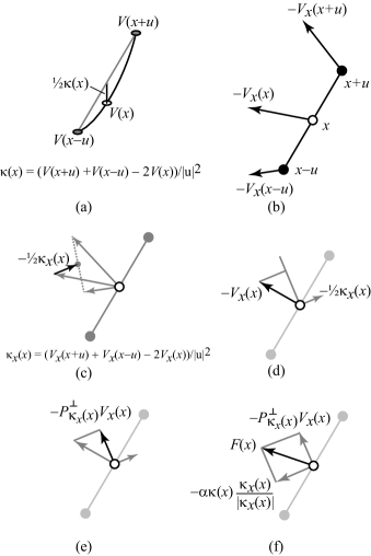
Figure 2: Computation steps of the outer optimization algorithm. Grey arrows represent results from the previous steps. (a) The curvature of the potential $\kappa(x)$ at $x$ can be estimated via the finite difference $\kappa(x)=\left(V(x+u(x))+V(x-u(x))-2V(x)\right)/\left|u\right|^{2}$. The algorithm also exploits the knowledge of the forces (b) acting at points $x+u$, $x-u$ and $x$ to form the finite difference $\kappa_{x}(x)=\left(V_{x}(x+u(x))+V_{x}(x-u(x))-2V_{x}(x)\right)/\left|u\right|^{2}$, which yields an estimate of the gradient of the curvature (c). The force $-V_{x}(x)$ (d) is then projected orthogonally (e) to $\kappa_{x}(x)$ to yield $-P_{\kappa_{x}\left(x\right)}^{\perp}V_{x}\left(x\right)$. Moving in this direction ensures that the curvature constraint $\kappa\left(x\right)=0$ is maintained, to first order, while the energy is being minimized. (f) To generate an explicit driving force towards points $x$ that satisfy the constraint $\kappa\left(x\right)=0$, the total “force” $F\left(x\right)$ acting on the system is obtained by adding the contribution from (e) to an attractive force towards the hyperplane where the constraint is satisfied. The latter is obtained by combining the curvature information from step (a) and the curvature gradient direction from step (c). The parameter $\alpha$ controls the relative strengths of the constraint stringency force and of the energy minimizing force.

If one happens to start the optimization from a point such that $\kappa(x)=0$, then it is sufficient to move $x$ in the direction opposite to the gradient $V_{x}(x)$, projected orthogonal to $\kappa_{x}(x)$. This ensures that the constraint $\kappa(x)=0$ remains satisfied (to first order) as the energy is being minimized. During a numerical optimization, however, the update steps are not infinitesimal, hence $\kappa(x)$ will gradually deviate from zero as the optimization progresses. To avoid this, we add a force, parallel to $\kappa_{x}(x)$, proportional in magnitude to $\kappa(x)$ and in a direction such that it brings the system back towards the hypersurface where $\kappa(x)=0$. This additional force also has the desirable side-effect that the constraint does not need to be already satisfied at the starting point of the optimization, since the method generates an attractive force towards the $\kappa(x)=0$ hypersurface.

The force acting on the system is then given by the sum of these two contributions:

$$F(x)=-P_{\kappa_{x}(x)}^{\perp}V_{x}(x)-\alpha\kappa(x)\frac{\kappa_{x}(x)}{|\kappa_{x}(x)|}$$ (1)

where $P_{v}^{\perp}=I-P_{v}^{\parallel}$, in which $P_{v}^{\parallel}=v(v^{T}v)^{-1}v^{T}$ is a matrix that projects onto the vector $v$, while $\alpha$ is a constant controlling the strength of the attraction to the constraint hyperplane. The force $F(x)$ can be fed into a standard gradient-driven optimization routine. Note that one can also arrive at Equation (1) via a standard Lagrange multiplier argument.

It is instructive to write the standard dimer method in a similar notation to emphasize the differences:

$$F\left(x\right)=-P_{u(x)}^{\perp}V_{x}(x)+P_{u(x)}^{\parallel}V_{x}(x)$$ (2)

where $u\left(x\right)$ is the direction of the dimer. Note that the gradient $V_{x}(x)$ is projected onto $u\left(x\right)$ in the dimer method instead of $\kappa_{x}\left(x\right)$ in our method. Also, the force along $\kappa_{x}(x)$ is determined by a simple projection of $V_{x}\left(x\right)$ onto $u$ in the dimer method rather than being jointly determined by the curvature $\kappa\left(x\right)$ and its gradient $\kappa_{x}\left(x\right)$.

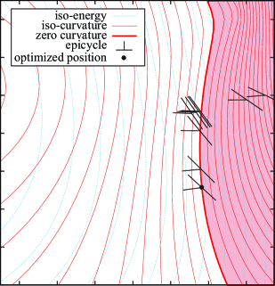
Figure 3: (Color online) Convergence of the proposed “inflection detection” method for the determination of inflection point. The figure shows contours of constant energy (which should be minimized) and contours of constant curvature (which is a constraint) for a test case involving a highly nonlinear analytic function. The dimer is shown as a “T” whose top line indicates the direction of smallest curvature and whose vertical line indicates the direction of largest curvature change. Conjugate gradient optimization steps are shown. The optimized position is seen to lie on a line of zero curvature at the point of minimum energy within the shaded region (in which the minimum curvature is negative).

Figure 3 shows a calculated inflection point in a simple analytic example (chosen to be two-dimensional, to enable a graphical representation) with the potential $V\left(x,y\right)=\left(x^{2}+y^{2}\right)/2-\left(x^{2}+y^{2}\right)^{3/2}/6+\sqrt{y}+x/8+3\exp\left(-\left(x-23/10\right)^{2}-\left(9/16\right)\left(y-0.5\right)^{2}\right)+x^{2}+y/5.$

II.1.4 Implementation details

A few aspects of the implementation deserve some attention. First, in the common situation of a periodic system, the state vector $x$ must also contain the degrees of freedom corresponding to the unit cell shape. To ensure that, regardless of the number of atoms in the unit cell, the entries in the variable $x$ have comparable magnitudes and the corresponding forces have comparable magnitude as well, we use the following scaling. The strain $\varepsilon_{ij}$ applied on the unit cell is stored in $x$ as a scaled strain $\tilde{\varepsilon}$, defined as

$$\tilde{\varepsilon}_{ij}=\gamma^{-1}n\Omega^{1/3}\varepsilon_{ij},$$ (3)

where $\Omega$ is the average volume per atom, $n$ is the number of atoms in the unit cell and $\gamma$ is a dimensionless user-specified parameter. The corresponding scaled stress $\tilde{\sigma}$ is given by

$$\tilde{\sigma}_{ij}=\gamma\Omega^{2/3}\sigma_{ij},$$ (4)

where $\sigma_{ij}$ is the actual stress. One can readily verify that the product of the two scaled conjugate variables is, as it should, $\gamma^{-1}n\Omega^{1/3}\varepsilon_{ij}\gamma\Omega^{2/3}\sigma_{ij}=V\varepsilon_{ij}\sigma_{ij}$, where $V=n\Omega$ is the cell volume. This convention offers the advantage that the scaled stress $\Omega^{2/3}\sigma_{ij}$ has units of force and its magnitude is independent of the cell size (since $\Omega$ is the volume per atom and not per cell). Also, the scaled strain $n\Omega^{1/3}\varepsilon_{ij}$ has units of length and ensures that, as the unit cell size $n$ increases, a given amount of scaled strain corresponds to a smaller actual strain. As a result, the change in energy corresponding to a given level of scaled strain does not grow with unit cell size.

A related issue is that, ideally, the atomic coordinates and forces should also be independent of cell size. Consequently, it is inconvenient to use fractional coordinates in the vector $x$ because a given level of scaled force could be associated with very different real magnitude of the forces if the unit cell is noncubic. To avoid this, we directly store the atoms’ cartesian coordinates in the vector $x$. We use their coordinates before the whole system is uniformly strained by the strain $\varepsilon$ (as this choice avoids complex coupling terms in the stress tensor). These scalings offer the advantages that the tolerance criterion for convergence can be specified in easy-to-interpret units and that it does not need to be adjusted for cell size.

It is important to realize that the method is only able to identify an unstable mode that can be represented with the supercell considered. It is possible that, once the onset of instability for a given supercell has been found, a full lattice dynamics analysis would reveal an unstable mode involving correlated motion over a cell bigger than the one considered. In such case, one can simply create a supercell that has the right size and shape in order to accommodate the unstable phonon mode (if there are multiple, it is advisable to consider the most unstable mode) and re-run our method on that supercell. Even though a lattice dynamics calculation is still necessary, we still avoid the need to perform a large number of such calculations, once for each trial geometry, thus considerably reducing the computational burden.

Equation (1) involves a user-specified stiffness parameter $\alpha$ (which can also be viewed as Lagrange multiplier). The method is theoretically valid for any value of $\alpha$, but different values merely weigh differently the stringency of the constraint versus the accuracy of the minimum energy. In practice, we set it to a reasonable value such that the two terms of Equation (1) have the same magnitude for the initial trial value of $x$. We then leave its value unchanged for the remaining iterations. This choice typically results in a fairly well conditioned optimization problem (with all terms in Equation (1) having similar orders of magnitudes). Although one might think that the value of $\alpha$ could be set automatically if one formally solved the constrained optimization problem via the Lagrange multiplier method, this is not the case: Multiplying the constraint $\kappa\left(x\right)=0$ by an arbitrary constant changes the conditioning of the Lagrangian optimization problem in the same way as changing the factor $\alpha$ does in our approach.

A few other important points that apply equally to the original dimer method should be kept in mind. The inner optimization problem is very well behaved because it corresponds to minimizing a quadratic form on a hypersphere. As a result, conjugate gradient methods perform very well and are quite robust. However, the outer optimization problem can be substantially more nonlinear. In addition, it is important to realize that the force obtained by Equation (1) is not, in general, guaranteed to be the exact gradient of some function. It does behave as a proper gradient in the limit of approaching the solution, however. These observations suggest that optimization methods that require function values (in addition to gradients) are not well suited to drive the outer optimization problem. Similarly, methods that rely on a quadratic form assumption should only be used for refinement, once a reasonably good solution has already been obtained. In our experience, performing a few steps of descent along the gradient is a good way to improve the initial guess of the solution before iterating a conjugate gradient algorithm to convergence.

An efficient implementation of the method should exploit the fact that the epicycle typically does not need to turn very much between two steps of the outer optimization algorithm (as is visible in Figure 3). That is, the direction of the most unstable mode varies smoothly with the structure’s geometry. As a result, the first invocation of the inner optimization problem will typically take about as long as a standard structural relaxation in order to find the most unstable mode but subsequent invocation will typically only demand the equivalent of a few static calculations.

To reach a given energy accuracy, the number of steps in the outer optimization routine tends to be slightly larger than the number of steps needed in a standard structural relaxation. This is due to the fact that the energy is quadratic in the atomic displacements near a minimum while the energy is linear in those displacements near an inflection point. As a result, the energy is less sensitive to a precise structural optimization near a minimum than near an inflection point and fewer optimization steps are thus needed in the former problem than in the latter. The net effect is that the computational cost of the proposed method is just a few times larger than the cost of a standard energy minimization.

When interfacing the method with a given total-energy ab initio code, a few more practical issues need some attention. First, it is crucial that all electronic structure calculations be carried out with constant basis set and the same $k$-points. Otherwise some of the numerical derivatives fail to behave smoothly, which may confuse the numerical optimization routines. Second, considerable efficiency improvements can be achieved if the ab initio code can exploit charge density prediction and re-use previously converged wavefunctions.

The above algorithm has been implemented as a C++ code and is now included in the Alloy Theoretic Automated Toolkit (ATAT) van de Walle and Ceder (2002); van de Walle et al. (2002); van de Walle (2009) (the key commands are infdet and robustrelax_vasp). The algorithm can thus easily be interfaced with any of the ab initio codes supported by ATAT. In the present work, we used the VASP ab initio code Kresse and Furthmüller (1996a, b); Kresse and Joubert (1999) and the interface to that code is more developed. For instance, helper routines automatically prepare some of the input files, copy files to re-use pre-converged results, ensure that a constant basis set is used (the present implementation of VASP’s constant basis set restarts require the user to specify the plane wave basis explicitly — our interface takes care of this.), etc.

III Examples

All structural optimizations reported below are driven by forces obtained from electronic structure calculations performed with VASP Kresse and Furthmüller (1996a, b); Kresse and Joubert (1999) in conjunction with the ATAT package van de Walle et al. (2002); van de Walle (2009); van de Walle et al. (2013) to model random solid solutions and the Phonopy software Togo and Tanaka (2015) to calculate phonon spectra. More computational details are given in the Appendix.

III.1 Failure mechanism of graphene under tension

The behavior of graphene under tension at the limit of its ideal strength has recently been studied in detail Marianetti and Yevick (2010) with the unexpected finding that the mechanical instability does not develop along the direction in which the strain is applied but instead involves the appearance of an unstable optical mode. This unexpected finding provides a compelling example of the usefulness of our approach, as it is specifically designed to efficiently explore all possible instabilities without performing a full lattice dynamics analysis at each trial configuration.

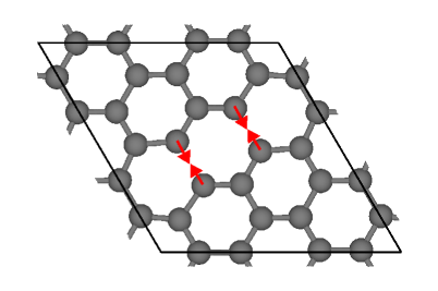
Figure 4: (Color online) Geometry of graphene at the limit of mechanical stability. Unit cell shown by a thick outline. Arrows indicate the most significant displacements associated with the unstable mode.

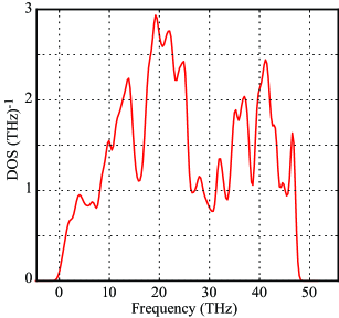
Figure 5: (Color online) Phonon Density of States (DOS) of graphene at the limit of its mechanical stability.

Our method provides a different perspective on this phenomena rather than merely corroborating the earlier finding. Our approach accounts for the fact that above absolute zero the system would visit many states in the neighborhood of its ideal high-symmetry crystal structure. Consequently, the point of mechanical instability would not necessarily be uniformly strained version of graphene’s ideal crystal structure. We find that, if thermal noise is accounted for, the system quickly breaks its symmetry and an unstable mode develops at a low strain (principal strains: 3.1% and 4.6%) about a low-symmetry structure rather than at a higher strain about a high-symmetry structure. The method delivers the point of lowest energy that lies on the edge of the domain of mechanical stability, thus discovering the “weakest link” of the material’s stability, instead of finding the location where a phonon instability develops along a given pre-specified path. Note that one can recover the earlier results Marianetti and Yevick (2010) by simply constraining the outer optimization problem to only explore isotropically strained version of the ideal graphene structure.

To identify the onset of instability, we first ran the method on a small supercell of 6 atoms, selected to match the supercell of the known unstable mode identified earlier Marianetti and Yevick (2010). Our method found an onset of instability for a mode that breaks exactly one bond per supercell of 6 atoms. A phonon analysis of this structure revealed an unstable phonon branch with a minimum at the Brillouin zone boundary. We thus created a supercell of 24 atoms that could represent this most unstable mode. Our method then found the structure depicted in Figure 4 and a lattice dynamics analysis no longer indicated any unstable modes (see Figure 5). The “weakest link” mode identified takes the form of the simultaneous breaking of two nearby bonds, repeated in a periodic pattern that appears to minimize the distortion of other bonds. This geometry could not have been anticipated from simple geometric or chemical arguments, which illustrates the usefulness of the method.

III.2 Free energy of mechanically unstable phases

It has recently been shown van de Walle et al. (2015) that the point of lowest energy at the onset of mechanical instability (as identified with the proposed method) provides a logically consistent definition of the energy of a mechanically unstable phase. For completeness and clarity, we summarize the main features of this approach below (refer to Figure 6). The set of coordinates $x$ such that $\kappa(x)>0$ and $\kappa(x)\leq 0$ correspond to mechanically stable and unstable regions, respectively. Given an ideal structure $x^{u}$ in which atoms are not allowed to relax away from their ideal positions, we define its neighborhood $\eta$ as the largest connected set containing $x^{u}$ over which the minimum curvature $\kappa(x)$ does not change sign. Now, we define the energy $E$ associated with $x^{u}$ as the minimum of the potential $V\left(x\right)$ over all $x$ in the neighborhood $\eta$. When $x^{u}$ is in a mechanically stable region, $E$ is just the potential energy $V\left(x^{r}\right)$ at the lowest local interior minimum $x^{r}$ in $\eta$, which agrees with the usual notion of energy of a relaxed structure. When $x^{u}$ is in a mechanically unstable region, $E=V\left(x^{r}\right)$ as well, but now $x^{r}$ must be at the boundary of $\eta$, i.e., a point where $\kappa(x)$ is zero. Specifically, $x^{r}$ is the point of minimum energy subject to the constraint that $\kappa\left(x^{r}\right)=0$. This definition offers three desirable properties: (i) it is based on a simple geometrical notion of curvature (ii) it can be shown that, at the onset of mechanical instability, a local minima always merges with a point of zero minimum curvature, so energy is a continuous function even across an instability and (iii) the relaxed structure $x^{r}$ is such that it is only unstable along at most a small finite number of modes (which is negligible in the thermodynamic limit of an infinite number of modes), so a standard lattice dynamics calculation can be used to calculate the free energy. This method is called “inflection detection” because $x^{r}$ lies at an inflection point for a mechanically unstable structure.

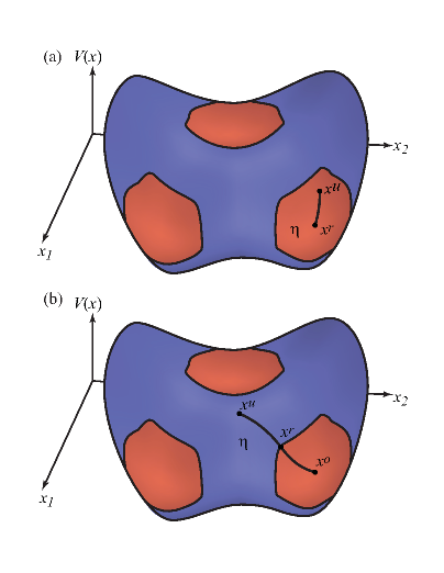
Figure 6: (Color online) Inflection-detection method. The potential energy hypersurface $V(x)$ (as a function of the state $x$ of the system) defines a natural partitioning of phase space into neighborhoods $\eta$, based on the sign of $\kappa\left(x\right)$, the local minimum curvature of $V(x)$ (blue: negative, red: positive). Each neighborhood (stable or not) can be assigned a well-defined energy by finding the minimum energy within that neighborhood. (a) In the case of a mechanically stable structure, the initial unrelaxed structure $x^{u}$ simply relaxes to a local minimum $x^{r}$. (b) For a mechanically unstable structure, an unconstrained minimization would yield the over-relaxed point $x^{o}$ which is actually the energy of another structure. The inflection detection method instead finds $x^{r}$, the minimum energy within $\eta$, which is located at an inflection point where the minimum curvature $\kappa\left(x\right)$ changes sign.

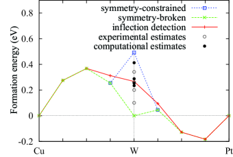
Figure 7: (Color online) Composition-dependence of the formation energy in the Cu-W and Pt-W fcc alloy systems. Symmetry-constrained results employ structural relaxations that preserve the initial symmetry of the structure while symmetry-broken ones allow the system to relax to its unconstrained minimum energy. Inflection-detection results represent either a local minimum or an inflection point energy, depending on which one is closest to the initial unrelaxed structure. The inflection-detection graph is seen to be the only one that generates a smooth behavior across all compositions that furthermore converges to a common value for the element W that both alloy systems share. This value compares favorably with available experimentalGuillermet et al. (1995); Saunders et al. (1988); Dinsdale (1991); Kaufman and Bernstein (1970) and computationalOzolins (2009); van de Walle et al. (2015) estimates.

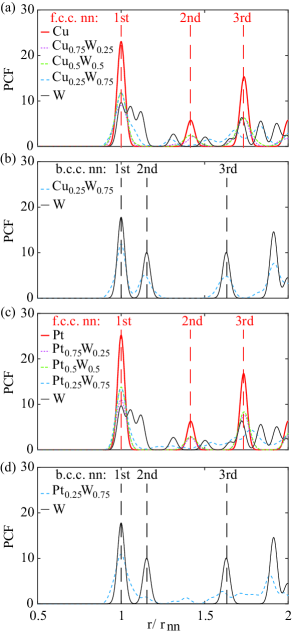
Figure 8: (Color online) Pair correlartion functions (PCF) for various disordered alloy systems: (a) fcc Cu_xW_1-x, (b) bcc Cu_xW_1-x, (c) fcc Pt_xW_1-x and (d) bcc Pt_xW_1-x. For fcc structures with $x\leq 0.25$, the structure geometries correspond to the inflection point determined with the proposed algorithm. In all other cases, the structure geometries correspond to local minima.

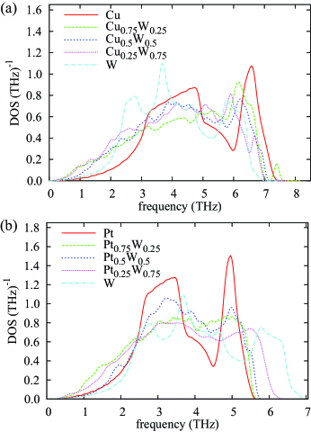
Figure 9: (Color online) Composition-dependence of the phonon Density of States (DOS) in the (a) Cu-W and (b) Pt-W fcc alloy systems.

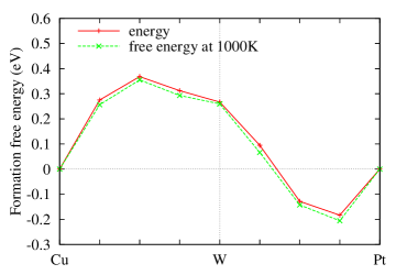
Figure 10: (Color online) Composition-dependence of the formation energy and free energy (at 1000 K) in the Cu-W and Pt-W fcc alloy systems.

The inflection point calculations presented in van de Walle et al. (2015) relied on the Nudged Elastic Band Method (NEB) H. Jonsson and Jacobsen (1998), which has two drawbacks in the context of inflection point calculations. First, this approach demands rather large-scale calculations in which multiple copies of the whole system are being simultaneously optimized to map out the path along the elastic band. Second, this method is only sensitive to instabilities that develop along the path and not perpendicular to it. In contrast, the method proposed here enables the efficient calculation of the inflection point using only one image of the whole system and is sensitive to instabilities along any of the phonon modes (that can be represented within the supercell used).

In this application, we have found that a reasonable starting point for the algorithm can be obtained from the midpoint between a fully relaxed structure (allowing cell parameters and ionic positions to vary) and a constrained relaxation in which only the isotropic changes in the unit cell are allowed (i.e. a “volume only” relaxation).

As an illustration, we compute formation energies of mechanically unstable phases fcc solid solutions in the Cu-W and Pt-W systems, which share the W component, whose stable structure is bcc, while the stable structure of Cu and Pt is fcc. The disordered alloys in these systems are modeled via Special Quasirandom Structures (SQS) Zunger et al. (1990) generated with the mcsqs code van de Walle et al. (2013) of the ATAT package van de Walle et al. (2002); van de Walle (2009).

Figure 7 shows formation energies (relative to a phase-separated mixture of fcc Cu, fcc Pt and bcc W of the same overall composition) as a function of composition computed in various ways. The symmetry-constrained result is obtained by performing structural relaxations that preserve the initial symmetry of the structure before the relaxation steps (which is the default behavior for most ab initio codes). The symmetry-broken results are equivalent to the symmetry-constrained ones, except for mechanically unstable high-symmetry structures (here fcc W), where the symmetry is explicitly broken to allow the system to relax to its unconstrained minimum energy (here bcc W). The latter scheme avoids mechanical instabilities but has the undesirable consequence that fcc W is actually assigned the energy of bcc W. Finally, the inflection detection curve is obtained by minimizing energy until one finds either a local minimum or an inflection point, and reporting the energy of whichever is first found. (Another way to describe the approach is to state that one uses fully relaxed energies for all structures that maintain an fcc-type coordination upon relaxation and inflection point energies for structures that do not.)

In the Cu-W binary, the fcc structure is thermodynamically unstable at all but very dilute compositions (as indicated by the positive formation energies). However, the fcc structure is nevertheless mechanically stable at least up to 50 atomic % W. The data point at 75 atomic % W clearly exhibits mechanical instability (since the relaxed and inflection detection results differ). This is also visible in Figure 8, which shows the pair correlation functions (PCF) for each structure. For Cu, Cu_0.75W_0.25 and Cu_0.5W_0.5, the PCF is clearly indicative of an fcc structure (see Figure 8(a)). For Cu_0.25W_0.75 and W, the fully relaxed structures exhibit a bcc-like PCF, as shown in Figure 8(b). For these structures, we thus use the inflection detection method and the resulting PCF, shown in Figure 8(a), are almost fcc-like: The first nearest neighbor peak is at the same distance, although it is a bit broadened, especially for W. The second nearest neighbor peak splits into two peaks whose centers average to the corresponding fcc peak.

In the Pt-W binary, the fcc structure is mechanically stable for a broad range of compositions, as can be seen from the fact that all three methods agree for most data points in Figure 7 and the fact that the corresponding PCF, shown in Figure 8(c) are fcc-like. The points at 75 atomic % W is relaxing to a bcc-like structure (as indicated by the PCF shown in Figure 8(d), although the second nearest neighbor peaks are not as well defined as for Cu_0.25W_0.75). For this point, the inflection detection method also yields a fcc-like PCF (see Figure 8(c)) similar to Cu_0.25W_0.75.

In Figure 7, we show the composition dependence of the energy in both systems on a common graph to demonstrate that the energies of both alloys smoothly converge to an identical value for the common element W in the (virtual) fcc structure. Interestingly, this value of the energy of fcc W is very consistent with previous estimates Guillermet et al. (1995); Saunders et al. (1988); Dinsdale (1991); Kaufman and Bernstein (1970); Ozolins (2009): It falls roughly in the middle of the cloud of estimates and at a location where there is an increased density of earlier data points. It is interesting to observe that, if one only looked at the Pt-W system, one may be led to believe that using symmetry-constrained energy is the “right” approach while if one only looked at the Cu-W system, one would think that using symmetry-broken energies is the “right” approach. But these two approaches would yield different values for the W energy. In contrast, the inflection detection approach, which also yields a smooth behavior for both systems, converges to a common value for the pure element W for both systems.

The inflection detection method also guarantees that all phonon modes but one are stable, a property that can be independently verified by lattice dynamics calculations (see Figure 9). This property enables the calculation of phonon free energy contributions via a standard harmonic treatment. As shown in Figure 10, the resulting free energies also vary smoothly with composition, reflecting the relatively smooth composition-dependence of the DOS (see Figure 9). The free energies as a function of composition also converge to a common value for pure W, as seen in Figure 10. Note that the configurational entropy is deliberately excluded in this graph because its singular behavior (of the form $X\ln X$ as $X\rightarrow 0$) near pure compositions would mask the smoothness of the phonon contributions.

IV Conclusion

We have devised a formal method to determine the point of minimum energy lying at the onset of mechanical stability. Exploiting some of the same principles underlying the well-known dimer method, our approach avoids the need to compute higher order derivatives of the energy (as only forces are needed). However, our method differs in nontrivial ways from the dimer method because it seeks minimum energy inflection points rather than saddle points.

Our method proves useful in investigating the mechanisms for mechanical failure at the atomic level, as illustrated in the case of graphene. Our example of application to Cu-W and Pt-W disordered alloys also support the proposal van de Walle et al. (2015) that the determination of the lowest energy inflection point provides a reliable, well-defined and computationally convenient way to assign energies to mechanically unstable phases. The proposed method makes this approach even more attractive, because the computational cost associated with finding the inflection point is just a few times larger than that of a standard structural relaxation. An implementation of the proposed method is now part of the ATAT package van de Walle et al. (2002); van de Walle (2009) (as the command “infdet” or the script “robustrelax_vasp”).

*

Appendix A Computational Methods Details

Electronic structure calculations are performed with VASP Kresse and Furthmüller (1996a, b); Kresse and Joubert (1999) using the PBE exchange-correlation functional Perdew et al. (1996) and Projector-Augmented Wave (PAW) Blöchl (1994) pseudopotentials. The precision flag is set to “high” (which specifies the kinetic energy cutoff) while the number of $k$-point is set to $4000$ per reciprocal atom (see van de Walle and Ceder (2002) for a description of this convention) with a Gaussian smearing of 0.1 eV (for force calculations) and the tetrahedron method with Blöchl corrections for total energies. The energy convergence criterion of $10^{-5}$ eV is used.

The SQS used to model random solid solution were generated with the mcsqs tool van de Walle et al. (2013) of the ATAT package van de Walle et al. (2002); van de Walle (2009). The SQS used are those included in the package’s distribution and have a unit cell of 32 atoms. These SQS match the pair correlations of the disordered state up to third nearest neighbor as well as the triplet correlations at least up to the second nearest neighbor.

The epicycle length for the inflection detection algorithm is set to $\epsilon=$ $0.2$ Šand the user-specified factor for scaling the strain and stress in Equations (3) and (4) is $\gamma=3$. The parameter $\alpha$ in Equation (1) is set automatically, as described in Section II.1.4 and its value ranged from $\alpha\approx 3$ to $\alpha\approx 200$ in our applications, depending of the system. The method was iterated to yield an energy accuracy better than $1$ meV/atom and a curvature accuracy better than $0.02$ eV/Ų.

Lattice dynamics calculations are performed with the Phonopy software Togo and Tanaka (2015). For the lattice dynamics calculations of graphene, 144 force calculations are performed on a 96-atom unit cell (a $2\times 2\times 1$ supercell of the 24-atom cell mentioned in Section III.1) with a $k$-point mesh of $3\times 3\times 1$ and imposed displacement of 0.01 Å. For each displacement, a displacement in the exact opposite direction is also considered, to cancel out the effect of any nonzero gradient on the calculation of the Hessian. A phonon $k$-point mesh of $11\times 11\times 1$ is used. For the lattice dynamics calculations of Cu-W and Pt-W alloys, the force calculations employ symmetrically distinct displacements of 0.015 Å. For simple fcc or bcc structures, a $3\times 3\times 3$ supercells is used while for SQS the supercell is either the structure’s unit cell (for large 32-atom SQS), or, in some cases (Cu_0.25W_0.75 and Pt_0.25W_0.75), a $2\times 1\times 1$ supercell (consisting of 64 atoms) of the SQS unit cell. A phonon $k$-point mesh of $21\times 21\times 21$ is used.

References

- Grimvall et al. (2012) G. Grimvall, B. Magyari-Köpe, C. Ozolins, and K. A. Persson, Rev. Mod. Phys. 84, 945 (2012).
- Luo et al. (2002) W. Luo, D. Roundy, M. L. Cohen, and J. W. Morris, Phys. Rev. B 66, 094110 (2002).
- Marianetti and Yevick (2010) C. Marianetti and H. Yevick, Phys. Rev. Lett. 105, 245502 (2010).
- van de Walle et al. (2015) A. van de Walle, Q.-J. Hong, S. Kadkhodaei, and R. Sun, Nature Commun. 6, 7559 (2015).
- Henkelman and Jonsson (1999) G. Henkelman and H. Jonsson, J. Chem. Phys. 111, 7010 (1999).
- Voter (1997) A. F. Voter, Phys. Rev. Lett. 78, 3908 (1997).
- Fletcher and Reeves (1964) R. Fletcher and C. M. Reeves, Comput. J. 7, 149 (1964).
- van de Walle and Ceder (2002) A. van de Walle and G. Ceder, J. Phase Equilib. 23, 348 (2002).
- van de Walle et al. (2002) A. van de Walle, M. D. Asta, and G. Ceder, Calphad 26, 539 (2002).
- van de Walle (2009) A. van de Walle, Calphad 33, 266 (2009).
- Kresse and Furthmüller (1996a) G. Kresse and J. Furthmüller, Phys. Rev. B 54, 11169 (1996a).
- Kresse and Furthmüller (1996b) G. Kresse and J. Furthmüller, Comp. Mater. Sci. 6, 15 (1996b).
- Kresse and Joubert (1999) G. Kresse and D. Joubert, Phys. Rev. B 59, 1758 (1999).
- van de Walle et al. (2013) A. van de Walle, P. Tiwary, M. M. de Jong, D. L. Olmsted, M. D. Asta, A. Dick, D. Shin, Y. Wang, L.-Q. Chen, and Z.-K. Liu, Calphad 42, 13 (2013).
- Togo and Tanaka (2015) A. Togo and I. Tanaka, Scr. Mater. 108, 1 (2015).
- H. Jonsson and Jacobsen (1998) G. M. H. Jonsson and K. W. Jacobsen, in Classical and Quantum Dynamics in Condensed Phase Simulations, edited by B. J. Berne, G. Ciccotti, and D. F. Coker (World Scientific, 1998).
- Zunger et al. (1990) A. Zunger, S.-H. Wei, L. Ferreira, and J. E. Bernard, Phys. Rev. Lett. 65, 353 (1990).
- Guillermet et al. (1995) A. F. Guillermet, V. Ozolins, G. Grimvall, and M. Körling, Phys. Rev. B 51, 10364 (1995).
- Saunders et al. (1988) N. Saunders, A. Miodownik, and A. Dinsdale, Calphad 12, 351 (1988).
- Dinsdale (1991) A. T. Dinsdale, Calphad 15, 317 (1991).
- Kaufman and Bernstein (1970) L. Kaufman and H. Bernstein, Computer Calculation of Phase Diagrams (Academic Press, New York, 1970).
- Ozolins (2009) V. Ozolins, Phys. Rev. Lett. 102, 065702 (2009).
- Perdew et al. (1996) J. P. Perdew, K. Burke, and M. Ernzerhof, Phys. Rev. Lett. 77, 3865 (1996).
- Blöchl (1994) P. E. Blöchl, Phys. Rev. B 50, 17953 (1994).
*