Nodal and nodeless gap in proximity induced superconductivity: application to monolayer CuO₂ on BSCCO substrate

Abstract

We present a detailed analysis on the hopping between monolayer CuO₂ and bulk CuO₂ plane in the Bi₂Sr₂CaCu₂O_8+δ substrate. With a two-band model, we demonstrate that the nodeless gap can only exist when the hole concentration in monolayer CuO₂ plane is very large. We argue that the possible phase separation may play important role in the recent experimental observation of nodeless gap.

I INTRODUCTION

The high temperature cuprate superconductor is one of the most important fields in past thirty yearsmuller_bednorz ; RVB ; Zhang_rice ; plain_vanilla ; Lee_Nagaosa_Wen ; review . Though the mechanism of the high Tc superconductivity in these materials is still under debate, physicists have reached some consensus, such that the physics is dominated by CuO₂ plane, and the superconductivity gap has d-wave pairing symmetry and so on review . However, in a recent experiment, Zhong et. al. observed a nodeless U-shape gap with STM on a monolayer CuO₂[CuO(1)] plane grown on a Bi₂Sr₂CaCu₂O_8+δ(BSCCO) substrates with MBE technique xue . They also found that the U-shape gap is robust against impurity scattering and closed at a temperature near the Tc of the substrates. This observation suggests a nodeless superconducting gap in the CuO(1) plane. However, it is contradict with the well accepted d-wave pairing symmetry in cuprate which has four nodes and V-shape gap in local density of states.

Soon after the experiment, Zhu et al. proposed that the almost same Tc between CuO(1) layer and BSCCO suggests the superconducting gap observed in CuO(1) layer is induced by proximity effect, while the gap is U-shape because of the multi-band nature in the CuO(1) layerzhu . They argued that the hole transfer between the surface CuO(1) layer and bulk BSCCO is not significant, so the substrate remains charge neutral, while the hole concentration in CuO(1) is one hole per oxygen. Thus the hole concentration in CuO(1) is much larger than the one in CuO₂ plane in the cuprate. Such a large hole doping makes CuO(1) layer a good metal instead of a doped Mott insulator. So instead of the t-J model based on Zhang-Rice singlet, Zhu et al. considered a phenomenological two-band model of oxygen 2p_x and 2p_y orbitals with proximity induced intraorbital pairings. The pairing was described by three phenomenological parameters $\Delta_{0}$, $\Delta_{x}$, and $\Delta_{y}$ corresponding to on-site and next nearest neighbor (NNN) pairing between two oxygen 2p_x orbitals or two 2p_y orbitals respectively. They studied the case where both $\Delta_{0}$ and $\Delta_{x}+\Delta_{y}$ are positive, and their results showed that a nodeless gap could be induced when $\Delta_{0}$ is large and inter-orbital hopping is small at various electron density (0.6, 0.695, and 0.815 electron per oxygen).

In this paper, we perform a detailed investigation on the proximity effect between the CuO(1) layer and the nearest CuO₂ layer in the BSCCO [CuO(2)]. We estimate the pairing terms up to 4th nearest neighbor(NN) pairing with a microscopic model. We find that the phenomenological parameter $\Delta_{0}$ and $\Delta_{x}+\Delta_{y}$ should have opposite signs which are not studied in ref zhu . Using the pairing parameters with opposite signs, we obtain a different phase diagram from Zhu et al. This result is a complementary to the calculation of Zhu et al. We also investigate the effect of 3rd NN and 4th NN terms. The phase diagram changes dramatically when 3rd NN term is included. When the pairing is not very weak, whether the gap is nodal or nodeless is determined by the chemical potential and is independent with the pairing strength. Our results show that one can only observe U-shape gap when the electron concentration is very low. Because the hole concentration in CuO(1) layer is around 1 hole per oxygen, our results suggest a phase separation in the CuO(1) layer, i.e. the hole concentration is very large in some region and very small in others. This is consistent with the experimental observation, where the U-shape gap is only observed in some regions while a pseudogap like behavior is observed in other regions. We also check the effect of interorbital pairing described by the 4th NN term, and the result shows that it is neglectable in terms of the phase diagram.

The paper is organized as follows. In Sec. II, we present our detailed analysis to proximity effect and introduce our model. In Sec. III, we discuss the numerical results of the phase diagrams and analyze the resultant phase diagrams based on analytical derivation. Our conclusions can be found in Sec. IV.

II MODEL

We start with a similar two-band model with the one used in ref. zhu ,

$$H =H_{0}+H_{p},$$ (1)

where $H_{0}$ describes the kinetic energy of CuO(1) layer and reads

$$H_{0} =\sum_{\alpha\beta\mathbf{k}\sigma}\epsilon_{\alpha\beta}(\mathbf{k})c_{\mathbf{k}\alpha\sigma}^{{\dagger}}c_{\mathbf{k}\beta\sigma}.$$ (2)

Here, $c_{\mathbf{k}\alpha\sigma}$ is the annihilation operator of electron with wavenumber $\mathbf{k}$ orbital $\alpha$ and spin $\sigma$. $\alpha,\beta=x,y$ are the orbital indices which correspond to oxygen $2p_{x}$ and $2p_{y}$ orbital respectively. Following Zhu et al. zhu , we consider the simplest case with NN and NNN hopping only,

$$\epsilon_{xx}(\mathbf{k}) =2(t_{x}\cos k_{x}+t_{y}\cos k_{y})-\mu$$

$$\epsilon_{yy}(\mathbf{k}) =2(t_{y}\cos k_{x}+t_{x}\cos k_{y})-\mu$$

$$\epsilon_{xy}(\mathbf{k}) =\epsilon_{yx}(\mathbf{k})=4t_{xy}\sin\frac{k_{x}}{2}\sin\frac{k_{y}}{2},$$ (3)

where $t_{x}$, $t_{y}$, and $t_{xy}$ are hopping integrals as shown in fig. 1(a), and $\mu$ is the chemical potential. Note that the different form of $\epsilon_{\alpha\beta}$ between the above and the one used in Zhu et al. is because of different choices of the orbital orientations.

Here, we consider a two-band model with oxygen 2p_x and 2p_y orbitals instead of t-J model or Hubbard model because the hole concentration in CuO(1) layer is much larger than the one in the usual CuO₂ layer of cuprate. The hole concentration is around 1 hole per oxygen in the former one and usually no more than 0.15 hole per oxygen in the latter one. It is more natural to start with the oxygen 2p bands instead of Zhang-Rice band. In this scenario, the electron configuration of Cu ion is still 3d⁹ and the electron on the Cu site behaves still like a localized spin. As pointed out by Zhu et al., the coupling between the spin on Cu and oxygen bands may lead to renormalizations of the hopping integrals as in Kondo lattice system zhu . Therefore in the calculations below, we treat them as phenomenological parameters instead of using the bare values.

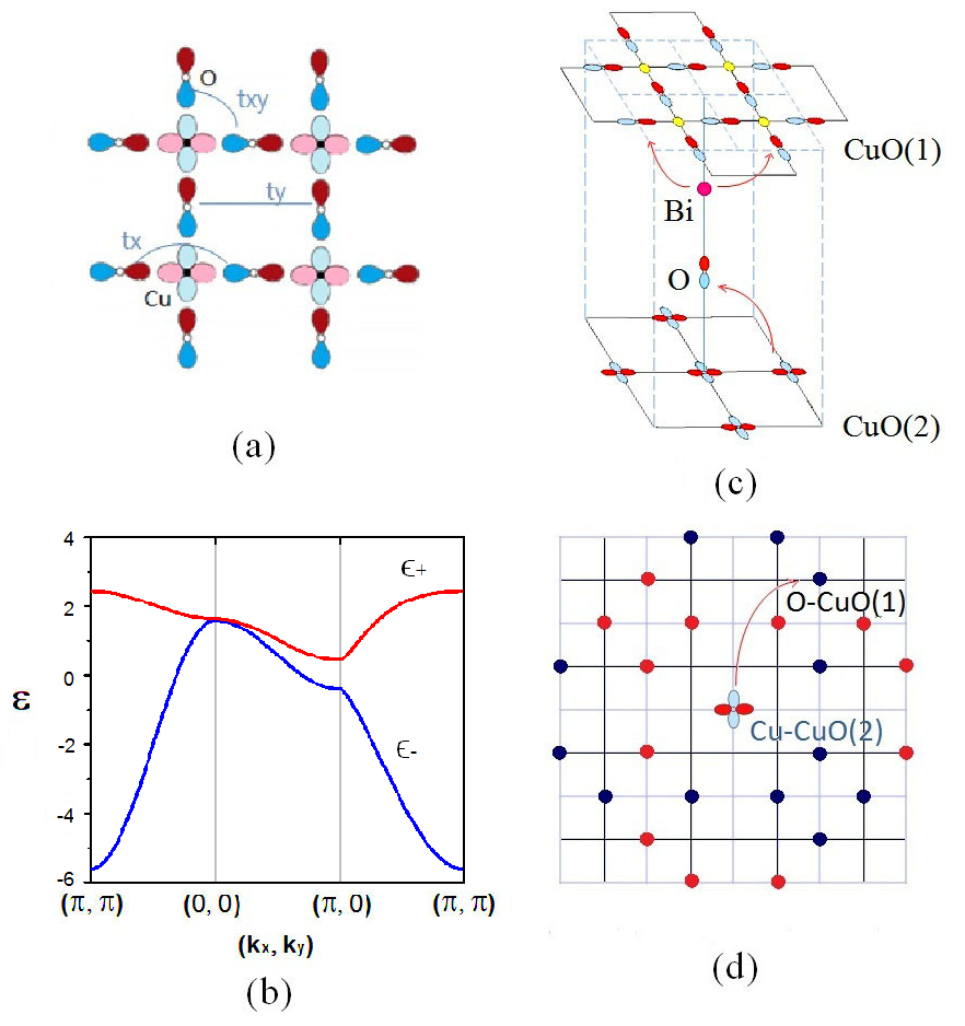
Figure 1: (a) The Schematic diagram of hopping integrals of the two band model. (b) The band structure with $t_{xy}=1$, $t_{x}=0.5$, and $t_{y}=0.3$. (c) the tunneling path between CuO(1) and CuO(2) layers. (d) The relative sign of the tunneling matrix element, red represents positive sign while black represents negative sign. See text for details.

As discussed in the introduction, the same Tc of CuO(1) and BSCCO substrate indicates that the superconductivity in CuO(1) is induced by proximity effect. So the pairing term $H_{p}$ reads

$$H_{p} =\frac{1}{2}\sum_{i\alpha,j\beta}\Delta^{*}_{\alpha\beta}(\mathbf{r}_{j}-\mathbf{r}_{i})(c_{i\alpha\uparrow}c_{j\beta\downarrow}-c_{i\alpha\downarrow}c_{j\beta\uparrow})+h.c,$$ (4)

where $\Delta_{\alpha\beta}$ tracks the proximity effect due to the CuO(2) layer. $\Delta_{\alpha\beta}$ should be proportional to the superconducting order parameter in CuO(2) layer and the tunneling matrix element between the two layers

$$\Delta_{\alpha\beta}(\mathbf{R}) \propto\sum_{i^{\prime}j^{\prime}\alpha\beta}T_{i\alpha,i^{\prime}}T_{i+\mathbf{R}\beta,j^{\prime}}\Delta^{(2)}_{i^{\prime}j^{\prime}},$$ (5)

where $T_{i\alpha,i^{\prime}}$ is the matrix element of tunneling between Cu 3d${}_{x^{2}-y^{2}}$ orbital at site $i^{\prime}$ in CuO(2) plane and the oxygen $\alpha$ orbital at site $i$ in CuO(1) plane, $\Delta^{(2)}_{i^{\prime}j^{\prime}}$ is the superconducting pairing of two holes at site $i^{\prime}$ and $j^{\prime}$ in CuO(2) layer. Because of the d-wave pairing in the CuO(2) plane, one have $\Delta^{(2)}_{i^{\prime}j^{\prime}}=\Delta^{(2)}(\delta_{j^{\prime},i^{\prime}\pm x}-\delta_{j^{\prime},i^{\prime}\pm y})$, where $\Delta^{(2)}$ is the d-wave pairing order parameter in CuO(2) plane. In the following, we choose the gauge that $\Delta^{(2)}$ is real.

Then we consider the tunneling matrix element $T_{i\alpha,i^{\prime}}$. Because of the large spatial distance between the two CuO₂ layers, direct hoppings are very difficult. Thus the hopping of a hole from CuO(2) to CuO(1) is consists of three steps $Cu\rightarrow O\rightarrow Bi\rightarrow O$ as shown in fig. 1(c). In the first step, a hole on Cu 3d${}_{x^{2}-y^{2}}$ orbital hops to an apical O 2p_z orbital in SrO plane. However, as pointed out by Yan Chen et al. yan , it is forbidden for a hole to hop to the 2p_z orbital of the oxygen just above it. A hole can only hop to nearest neighbor apical oxygen 2p_z orbitals as shown in fig. 1(c). In the second step, the hole hops from O 2p_z orbital to 6s orbital of the Bi just above it. Finally, it hops from Bi 6s orbital to O 2p_x/2p_y orbital in the monolayer CuO₂ in the third step. Similar to the first step, because Bi is in the center of each plaquette of the CuO(1), the direct hopping between Bi 6s orbital to nearest neighbor O 2p_x/2p_y orbitals is forbidden. Thus the hole hops from Bi to the eight next nearest neighbor O orbitals as shown in fig. 1(c).

In summary, a hole at a Cu 3d${}_{x^{2}-y^{2}}$ orbital in CuO(2) plane could hop to 24 different oxygen sites in CuO(1) plane as shown in fig. 1(d). It is obviously that all the $T_{i\alpha,i^{\prime}}$ for a given $i^{\prime}$ have same amplitude, but they may have different signs. Therefore we could define $T_{i\alpha,i^{\prime}}=s_{i\alpha,i^{\prime}}T_{0}$, where $T_{0}$ is the amplitude while $s$ tracks the sign. $T_{0}$ is hard to be calculated because of the lack of knowledge of the hopping details, while $s$ could be calculated based on the analysis of the orientations of the orbitals involved. In fig. 1(d), we depict $s$ for a given Cu site $i^{\prime}$, and the orientation of the orbitals are depicted in fig. 1(a) and (c). Note that in the analysis above, we assume that hole could only hop to 6s orbital of Bi. Because of the different sign structures between the 6p_z and 6s orbitals, their contributions to the tunneling matrix element $T_{i\alpha,i^{\prime}}$ have opposite signs. Therefore both $T_{0}$ and $s$ could change if the Bi 6p_z orbital is also involved in the hopping process. However, the relative sign between $s_{i\alpha,i^{\prime}}$ and $s_{j\beta,i^{\prime}}$ does not change, and we will show it below that only the relative sign is important.

Based on the analysis above, Eq. (5) could be rewritten as

$$\Delta_{\alpha\beta}(\mathbf{R})\propto\sum_{i^{\prime}j^{\prime}\alpha\beta}s_{i\alpha,i^{\prime}}s_{i+\mathbf{R}\beta,j^{\prime}}(\delta_{j^{\prime},i^{\prime}\pm x}-\delta_{j^{\prime},i^{\prime}\pm y}),$$ (6)

where $s$ is the sign due to the hopping of holes, and the term in the parenthesis tracks the d-wave pairing symmetry in the BSCCO substrate. It is obviously that only the relative sign of different $s$ is important. Our results show that a hole on one oxygen site could paired with another hole on up to 24th NN oxygen site. For simplicity, we consider only up to the 4th NN, and the Fourier’s transformation of $\Delta_{\alpha\beta}$ reads

$$\Delta_{xx}(k_{x},k_{y}) =-\Delta_{yy}(k_{y},k_{x})=\Delta_{0}+\Delta_{2}(k_{x},k_{y})+\Delta_{3}(k_{x},k_{y})$$

$$\Delta_{xy}(k_{x},k_{y}) =\Delta_{yx}(k_{y},k_{x})=\Delta_{4}(k_{x},k_{y}),$$

where $\Delta_{0}=24\Delta$, $\Delta_{2}(k_{x},k_{y})=48\Delta\cos k_{x}-32\Delta\cos k_{y}$, $\Delta_{3}(k_{x},k_{y})=-44\Delta\cos k_{x}\cos k_{y}$, and $\Delta_{4}(k_{x},k_{y})=20\Delta(\sin\frac{3k_{x}}{2}\sin\frac{k_{y}}{2}-\sin\frac{3k_{y}}{2}\sin\frac{k_{x}}{2})$ which correspond to on-site, NNN, 3rd NN, and 4th NN pairing respectively. Note that the NN term vanishes in above analysis. $\Delta$ is a parameter tracking the strength of the proximity effect. In previous study, Zhu et al. considered the $\Delta_{0}$, $\Delta_{2}$ terms by introducing three phenomenological parameters $\Delta_{0}$, $\Delta_{x}$ and $\Delta_{y}$. They analyzed the phase diagram with only positive $\Delta_{0}$ and $\Delta_{x}+\Delta_{y}$zhu . By comparing with their definitions, we find that the three parameters are $\Delta_{0}=24\Delta$, $\Delta_{x}=-24\Delta$ and $\Delta_{y}=16\Delta$ respectively. This leads to opposite sign between $\Delta_{0}$ and $\Delta_{x}+\Delta_{y}$ which is not discussed in their paper.

III Results and Analysis

By diagonalizing the Hamiltonian

$$H =\sum_{\mathbf{k}}\left(c^{{\dagger}}_{\mathbf{k}x\uparrow}c^{{\dagger}}_{\mathbf{k}y\uparrow}c_{-\mathbf{k}x\downarrow}c_{-\mathbf{k}y\downarrow}\right)\left(\begin{matrix}\epsilon_{xx}&\epsilon_{xy}&\Delta_{xx}&\Delta_{xy}\\ \epsilon_{xy}&\epsilon_{yy}&\Delta_{xy}&\Delta_{yy}\\ \Delta_{xx}&\Delta_{xy}&-\epsilon_{xx}&-\epsilon_{xy}\\ \Delta_{xy}&\Delta_{yy}&-\epsilon_{xy}&-\epsilon_{yy}\end{matrix}\right)\left(\begin{matrix}c_{\mathbf{k}x\uparrow}\\ c_{\mathbf{k}y\uparrow}\\ c^{{\dagger}}_{-\mathbf{k}x\downarrow}\\ c^{{\dagger}}_{-\mathbf{k}y\downarrow}\end{matrix}\right),$$ (7)

the quasiparticle energy reads

$$\pm E_{u}(\textbf{k}) =\pm\sqrt{\frac{A(\textbf{k})+\sqrt{A(\textbf{k})^{2}-4B(\textbf{k})}}{2}},$$

$$\pm E_{l}(\textbf{k}) =\pm\sqrt{\frac{A(\textbf{k})-\sqrt{A(\textbf{k})^{2}-4B(\textbf{k})}}{2}},$$

where $A(\mathbf{k})=\epsilon_{xx}^{2}+\epsilon_{yy}^{2}+2\epsilon_{xy}^{2}+\Delta_{xx}^{2}+\Delta_{yy}^{2}+2\Delta_{xy}^{2}$, and $B(\mathbf{k})=\left(\Delta_{xy}^{2}-\epsilon_{xy}^{2}+\epsilon_{xx}\epsilon_{yy}-\Delta_{xx}\Delta_{yy}\right)^{2}+\left(2\epsilon_{xy}\Delta_{xy}-\epsilon_{xx}\Delta_{yy}-\epsilon_{yy}\Delta_{xx}\right)^{2}$. The node of quasiparticle energy corresponds to $B(\mathbf{k})=0$ which requires

$$\Delta_{xy}^{2}-\epsilon_{xy}^{2}+\epsilon_{xx}\epsilon_{yy}-\Delta_{xx}\Delta_{yy}=0$$ (8)

$$2\epsilon_{xy}\Delta_{xy}-\epsilon_{xx}\Delta_{yy}-\epsilon_{yy}\Delta_{xx}=0.$$ (9)

The phase diagram can be calculated by solving these two equations. For a given set of parameters, the quasiparticle spectrum has node if one can find at least one solution of above equations, and it is nodeless if there is no solution for the above equations.

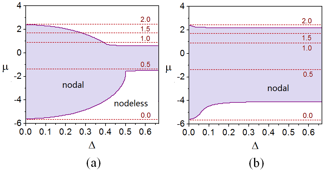
Figure 2: Phase diagram for nodal and nodeless superconducting gap with $t_{xy}=1,t_{x}=0.5,t_{y}=0.3.$. Dashed lines: the chemical potentials corresponds to 0, 0.5, 1, 1.5, and 2 electrons per oxygen respectively. (a) on-site and NNN terms only. (b) 3rd NN term is included.

At first, we consider the case with only on-site and NN terms where the interorbital pairing $\Delta_{xy}=0$. This is similar to the case studied in ref. zhu , except that $\Delta_{0}$ and $\Delta_{x}+\Delta_{y}$ have different signs now. To compare with the result of Zhu et al., we choose same set of parameters of hopping integrals, i.e. $t_{xy}=1$, $t_{x}=0.5$, and $t_{y}=0.3$. The corresponding band structure is presented in fig. 1(b), where $\epsilon_{\pm}=\frac{\epsilon_{x}+\epsilon_{y}}{2}\pm\frac{\sqrt{(\epsilon_{x}-\epsilon_{y})^{2}+4\epsilon_{xy}^{2}}}{2}$ is the dispersion of the two bands respectively. The resultant phase diagram is given in fig. 2(a). One could find that the region with a nodeless gap is rather small when $\Delta$ is small and enlarges with the increase of $\Delta$. However, even when the pairing term is rather large (note that on-site pairing $\Delta_{0}=24\Delta$), the gap is always V-shape for $-1.5<\mu<0.75$. This is different from Zhu et al.’s result where a nodeless gap could be observed when $\Delta_{0}$ is large for $\mu=0.2,-0.4,-0.8$.

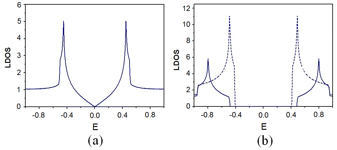
Figure 3: The quasi-particle local density of states at $\Delta=0.1,\mu=-5$. (a) on-site and NNN terms only, where the superconducting gap has nodes. (b) solid line: 3rd NN term is included; dashed line: both 3rd NN and 4th NN term are included. Both cases have nodeless gap.

The phase diagram changes dramatically when the 3rd NN term $\Delta_{3}$ is included as shown in fig. 2(b). In small $\Delta$ case, the nodeless region is slightly enlarged. For example, as shown in fig. 3 (a), with only $\Delta_{0}$ and $\Delta_{2}$, the local density of states at $\Delta=0.1$, $\mu=-5$ is V-shape, which indicates the existence of gap nodes. However, it becomes U-shape when $\Delta_{3}$ is included, as shown in fig. 3(b). Meanwhile, the nodeless region is strongly suppressed by $\Delta_{3}$ in large $\Delta$ case. According to fig. 2(b), when $\Delta>0.2$, the phase boundary is almost independent on $\Delta$, and a nodeless gap could be observed if and only if $\mu>2.24$ or $\mu<-4.08$ corresponding to less than $0.12$ hole per oxygen or less than $0.15$ electron per oxygen.

Figure 4: Left panel: lower branch of quasiparticle spectrum $E_{l}(\mathbf{k})$ in Brillouin zone. The white line is the Fermi surface. Middle panel: $E_{l}(\mathbf{k})$ on Fermi surface from point A to point B in (a) and (d) respectively. Right panel: $E_{l}(\mathbf{k})$ along diagonal direction. The parameters are $t_{x}=0.5$, $t_{y}=0.3$, $t_{xy}=1$, $\Delta=0.1$, $\mu=0.2$(upper panel) and $\mu=-5$ (lower panel).

To further investigate the property of the superconducting gap, we depict the lower branch of the quasiparticle spectrums $E_{l}(\mathbf{k})$ in whole Brillouin zone with $\Delta=0.1$ at $\mu=0.2$ (nodal gap region) and $\mu=-5$ (nodeless gap region) in fig. 4(a) and (d) respectively. The white line is the underlining Fermi surface. The $E_{l}(\mathbf{k})$ along Fermi surface are depicted in fig. 4(b) and (e) respectively. One interesting phenomenon is that there is no node on Fermi surface in $\mu=0.2$ case. Instead, the nodes of the quasiparticle dispersion are at points away from Fermi surface in the diagonal direction as shown in fig. 4(c). This is different from usual case where the nodes are always on the Fermi surface.

To understand these phenomena, we try to solve Eq. (8) and (9) analytically. We consider a special solution with $\cos k_{x}=\cos k_{y}$, i.e. $\mathbf{k}$ is along diagonal direction, then one has $\epsilon_{xx}=\epsilon_{yy}$ and $\Delta_{xx}=-\Delta_{yy}=(24+16\cos k_{x}-44\cos^{2}k_{x})\Delta$. Therefore Eq. (9) can be automatically satisfied in the case interorbital pairing $\Delta_{xy}$ vanishes. Then the Hamiltonian (7) in band basis reads

$$H =\sum_{\mathbf{k}}\left(c^{{\dagger}}_{\mathbf{k}(-)\uparrow}c^{{\dagger}}_{\mathbf{k}(+)\uparrow}c_{-\mathbf{k}(-)\downarrow}c_{-\mathbf{k}(+)\downarrow}\right)H(\mathbf{k})\left(\begin{matrix}c_{\mathbf{k}(-)\uparrow}\\ c_{\mathbf{k}(+)\uparrow}\\ c^{{\dagger}}_{-\mathbf{k}(-)\downarrow}\\ c^{{\dagger}}_{-\mathbf{k}(+)\downarrow}\end{matrix}\right),$$

with

$$H(\mathbf{k}) =\left(\begin{matrix}\epsilon_{-}-\mu&0&0&-\Delta_{xx}\\ 0&\epsilon_{+}-\mu&-\Delta_{xx}&0\\ 0&-\Delta_{xx}&-\epsilon_{-}+\mu&0\\ -\Delta_{xx}&0&0&-\epsilon_{+}+\mu\end{matrix}\right),$$ (10)

where $\epsilon_{\pm}(\mathbf{k})=2(t_{x}+t_{y})\cos k_{x}\pm|4t_{xy}\sin k_{x}/2\sin k_{y}/2|$ for $\cos k_{x}=\cos k_{y}$. Then the quasiparticle energy reads

$$\pm E_{u}(\textbf{k}) =\pm\left\{\delta{\epsilon}(\mathbf{k})+\sqrt{\left[\bar{\epsilon}(\mathbf{k})-\mu\right]^{2}+\Delta^{2}_{xx}(\mathbf{k})}\right\}.$$

$$\pm E_{l}(\textbf{k}) =\pm\left\{\delta{\epsilon}(\mathbf{k})-\sqrt{\left[\bar{\epsilon}(\mathbf{k})-\mu\right]^{2}+\Delta^{2}_{xx}(\mathbf{k})}\right\}.$$

where $\delta\epsilon=(\epsilon_{+}-\epsilon_{-})/2$ and $\bar{\epsilon}=(\epsilon_{+}+\epsilon_{-})/2$. Note that Eq. (10) indicates that the intraband pairing vanishes while the interband pairing dominants at diagonal direction. The interband pairing leads to the additional term $\delta\epsilon$ in the quasi-particle energy which is responsible for the shift of gap minimum away from Fermi surface.

Then we investigate the $\Delta$ independence of the phase boundary. This could be understood by considering the quasiparticle energy at three special k-points, $(\pi,\pi)$ and $\mathbf{k}_{\pm}$ where $\cos k_{x\pm}=\cos k_{y\pm}=\frac{2\pm\sqrt{70}}{11}$, and $\Delta_{xx}(\mathbf{k}_{\pm})=0$. It is obvious that $E_{l}(\mathbf{k}_{\pm})=\epsilon_{+}(\mathbf{k}_{\pm})-\mu$ if $\mu\geq\bar{\epsilon}$, and $E_{l}(\mathbf{k}_{\pm})=\mu-\epsilon_{-}(\mathbf{k}_{\pm})$ if $\mu<\bar{\epsilon}$. Therefore at least one of $E_{l}(\mathbf{k}_{\pm})$ is positive, if $\mu$ is between $\epsilon_{\pm}(\mathbf{k}_{+})$ or $\epsilon_{\pm}(\mathbf{k}_{-})$. On the other hand, $E(\pi,\pi)<0$ if $\Delta$ is large enough. This means that $E_{l}$ has at least one node if $\epsilon_{-}(\mathbf{k}_{+})\leq\mu\leq\epsilon_{+}(\mathbf{k}_{+})$ or $\epsilon_{-}(\mathbf{k}_{-})\leq\mu\leq\epsilon_{+}(\mathbf{k}_{-})$ when $\Delta$ is large enough. In fig. 5(a), we depict the phase boundary for chemical potential at $\Delta=1$, $t_{xy}=1$, $t_{x}=0.5$, and $t_{y}=0.3$. It is consistent with our analysis very well.

Figure 5: (a) $k_{\pm}$ and $\epsilon_{\pm}(k_{\pm},k_{\pm})$ for $t_{xy}=1,t_{x}=0.5,t_{y}=0.3$. The dashed line is the phase boundary between nodal and nodeless region. (b) the phase diagram at $\Delta=1$ and $t_{x}+t_{y}=0.8$. The dashed line is given by $\max[\epsilon_{+}(k_{+},k_{+}),\epsilon_{+}(k_{-},k_{-})]$ and $\min[\epsilon_{-}(k_{+},k_{+}),\epsilon_{-}(k_{-},k_{-})]$. See text for details.

Since the phase boundary of the nodeless region depends only on the $\epsilon_{\pm}(\mathbf{k}_{\pm})$ in diagonal direction, it depends only on the ratio of $t_{xy}/(t_{x}+t_{y})$. Thus we perform similar calculations for various $t_{xy}$ with $t_{x}+t_{y}=0.8$ and $\Delta=1$ to check the effect of kinetic energy. The results are presented in fig. 5(b) where the SC gap is nodal if $\mu$ lies in the blue region, and nodeless if $\mu$ lies in the red region. The dashed lines are given by $\max[\epsilon_{+}(k_{+},k_{+}),\epsilon_{+}(k_{-},k_{-})]$ and $\min[\epsilon_{-}(k_{+},k_{+}),\epsilon_{-}(k_{-},k_{-})]$. They coincide very well with the phase boundary from numerical calculations. According to the figure, the gap could be nodeless only when $\mu$ is close to top of the $\epsilon_{+}$ band or the bottom of the $\epsilon_{-}$ band.

Finally, we also include the 4th NN term $\Delta_{4}$ to study the effect of inter-orbital pairing. A typical result is shown as dashed line in fig. 3(b). Comparing to the result without 4th NN term (the solid line), the lineshape of the local density of states is different, and the gap is slightly suppressed, but the resultant phase diagram is almost the same as the one without $\Delta_{4}$. Therefore in terms of the phase diagram, the interorbital term $\Delta_{xy}$ can be safely ignored.

IV Summary and Discussions

We now discuss the possible relation between our results and the experimental observation of the nodeless gap in ref. xue . In our results, the nodeless gap can exist when the proximity pairing strength $\Delta_{0}$ is comparable to the hopping integrals. This is possible because of the renormalization of the oxygen band by coupling to localized spin on Cu, as discussed by Zhu et al.zhu . Our results also show that a nodeless gap could only exist at very large or very small hole concentrations. However, in the low hole concentration regime, the holes on oxygen will form Zhang-Rice singlets with the spins on Cu Zhang_rice , and the holes can be effectively considered as doped on Cu sites. Therefore our model is not valid in this case, which means that the low hole concentration regime should be excluded from consideration. Thus one can only have a nodeless gap when the hole concentrations is very large. This can not be satisfied if the monolayer CuO₂ is homogeneous because there is only 1 hole per oxygen. However, the experimental data shows that there are actually two kinds of regions, one has a large pseudogap-like V-shape gap, and the other has a superconducting U-shape gap xue . Therefore there may be a phase separation in the system, where one kind of region with low hole concentration exhibits psuedogap behavior, and the other kind with very large hole concentration exhibits nodeless superconducting gap.

In the calculations, a few assumptions have been introduced. For example, we have assumed that the charge transfer between the surface monolayer CuO₂ and the substrate is not significant. Therefore the average hole concentration in the CuO(1) is close to 1 hole per oxygen. We also assumed that the main effect of localized spins on Cu sites is to renormalize the oxygen bands through a Kondo lattice like physics, so we can consider an effective phenomenological model with only oxygen bands. Our analysis of the nodeless gap depends on these assumptions. Though these assumptions are difficult to check theoretically, they can be tested experimentally.

In summary, based on a detailed analysis of the hopping process for a hole between surface CuO₂ plane and an inner CuO₂ plane, we estimate the signs of the pairing parameters in the CuO₂ plane by using a phenomenological proximity Hamiltonian. Our calculation complete the proximity-induced-pairing scenario and show that nodeless gap could be induced only when the hole concentration on the monolayer CuO₂ is very large. This can give a further experimental test towards the proximity scenario. We argue that the nodeless gap could be related to the one observed in the experiment if there is phase separation in the monolayer CuO₂.

- (1) J. G. Bednorz and K. A. Muller, Z. Phys. B 64, 189 (1986).
- (2) P. W. Anderson, Science 235, 1196 (1987).
- (3) F.C. Zhang, T.M. Rice, Phys. Rev. B 37, 3759 (1988).
- (4) P. W. Anderson, P. A. Lee, M. Randeria, T. M. Rice, N. Trivedi, and F. C Zhang, J. Phys. Condens. Matter 16, R755 (2004).
- (5) P. A. Lee, N. Nagaosa, and X. G. Wen, Rev. Mod. Phys.78, 17 (2006).
- (6) For a recent review see B. Keimer, S. A. Kivelson, M. R. Norman, S. Uchida, and J. Zaanen, Nature 518, 179 (2015)
- (7) Yong Zhong, Yang Wang, Sha Han, Yan-Feng Lv, Wen-Lin Wang, Ding Zhang, Hao Ding, Yi-Min Zhang, Lili Wang, Ke He, Ruidan Zhong, John A. Schneeloch, Gen-Da Gu, Can-Li Song, Xu-Cun Ma, Qi-Kun Xue, Science Bulletin 2016, 61(16):1239-1247
- (8) Guo-Yi Zhu, Fu-Chun Zhang, and Guang-Ming Zhang, Phys. Rev. B 94, 174501 (2016)
- (9) Yan Chen, T. M. Rice, and F. C. Zhang, Phys. Rev. Lett. 97, 237004 (2006)