Response approach to the squeezed-limit bispectrum: application to the correlation of quasar and Lyman-$\alpha$ forest power spectrum

Abstract

The squeezed-limit bispectrum, which is generated by nonlinear gravitational evolution as well as inflationary physics, measures the correlation of three wavenumbers, in the configuration where one wavenumber is much smaller than the other two. Since the squeezed-limit bispectrum encodes the impact of a large-scale fluctuation on the small-scale power spectrum, it can be understood as how the small-scale power spectrum “responds” to the large-scale fluctuation. Viewed in this way, the squeezed-limit bispectrum can be calculated using the response approach even in the cases which do not submit to perturbative treatment. To illustrate this point, we apply this approach to the cross-correlation between the large-scale quasar density field and small-scale Lyman-$\alpha$ forest flux power spectrum. In particular, using separate universe simulations which implement changes in the large-scale density, velocity gradient, and primordial power spectrum amplitude, we measure how the Lyman-$\alpha$ forest flux power spectrum responds to the local, long-wavelength quasar overdensity, and equivalently their squeezed-limit bispectrum. We perform a Fisher forecast for the ability of future experiments to constrain local non-Gaussianity using the bispectrum of quasars and the Lyman-$\alpha$ forest. Combining with quasar and Lyman-$\alpha$ forest power spectra to constrain the biases, we find that for DESI the expected $1-\sigma$ constraint is ${\rm err}[f_{\rm NL}]\sim 60$. Ability for DESI to measure $f_{\rm NL}$ through this channel is limited primarily by the aliasing and instrumental noise of the Lyman-$\alpha$ forest flux power spectrum. The combination of response approach and separate universe simulations provides a novel technique to explore the constraints from the squeezed-limit bispectrum between different observables.

1 Introduction

The universe today is highly nonlinear, which renders making analytical or semi-analytical predictions a very hard problem even for the heavily simplified case of a universe made up of collisionless dark matter interacting through gravitational force alone. Luckily, the gravitational force is the only relevant long-range force in the universe and the curvature fluctuations are the only field that matters at the very large scales in the universe. This allows us to make surprisingly strong statements about properties of certain limits of correlators. The basic picture is that of a “separate universe.”

The separate universe picture posits that the evolution of a sufficiently large patch of the universe riding a large-scale overdensity is the same as that of a typical patch in a slightly overdense universe. In other words, we are making the approximation that the effect of a mode with sufficiently small wavenumber $k$ must approach that of the $k=0$ mode. On one hand, this approximation can be used in formal results [1, 2, 3, 4, 5]. On the other hand, there is ample evidence, from numerical experiments, that the information flow in the universe is strictly from the large scales to small scales, rather than the other way around [6, 7, 8, 9, 10, 11]. This means that in the sufficiently nonlinear regime, the small scales will contain remnant information of the large-scale phases, but the opposite is not true. This means that the separate universe picture works very well even in the limits where it is not expected to be formally exactly correct, i.e. it becomes an extremely good ansatz for the dominant dynamics of the system. This motivates entire trunks of research in the field and forms the basis of BAO reconstruction methods [12, 13] and the super-sample variance effects [14, 15, 16, 17].

This separate universe picture can also be straightforwardly implemented in cosmological $N$-body simulations, which is known as the separate universe simulations [18, 19, 16, 20], to study how the small-scale structure formation is affected by the large-scale density environment. Separate universe simulations have allowed for detailed studies on squeezed-limit $n$-point correlation function [21], the halo bias [22, 23, 24] (see Ref. [25] for a review), the $\text{Lyman-}\alpha$ forest [26, 27], and of the effect of other sectors that possess non-gravitational forces such as quintessence dark energy [28].

In this paper, we add to the canon by presenting explicit recipes for making predictions of the squeezed-limit bispectrum which couple one large-scale mode from one field and two small-scale modes from another (which can, but is not required to be the same as the first one). We consider the case most relevant for actual surveys: we take into account not only the possible large-scale density field, but also the redshift-space distortions and primordial non-Gaussianity of the local-type, which we hope to measure with exactly this kind of measurement. As a concrete example, we apply this method to the cross-correlation between the large-scale quasar field and small-scale $\text{Lyman-}\alpha$ forest field and perform a Fisher forecast for the ability of future experiments to constrain local non-Gaussianity using this bispectrum. Ref. [29] considered the constraint on local primordial non-Gaussianity using the $\text{Lyman-}\alpha$ forest flux bispectrum alone. However, as we shall argue in Section 5, the cross-correlation is generally more robust regarding systematics than the auto-correlation, and so may be more appealing.

The rest of the paper is organized as follows. In Section 2, we derive the relation between the power spectrum response and the squeezed-limit bispectrum, and then use the small-scale $\text{Lyman-}\alpha$ forest flux power spectrum and the large-scale quasar overdensity as an example. In Section 3, we introduce the separate universe simulations that are used to measure how the $\text{Lyman-}\alpha$ forest flux power spectrum responds to gravitational evolution and primordial non-Gaussianity. We then use the measured responses as well as the Fisher matrix to explore the constraining power on $f_{\rm NL}$ from the quasar–$\text{Lyman-}\alpha$ forest squeezed-limit bispectrum in Section 4. We conclude in Section 5.

2 Theory

2.1 Warming up: large-scale biasing to first order

We start by re-deriving some standard results as a warm-up. Consider a field $X$ (e.g. quasar overdensity field) with fluctuations on all scales. Its overdensity $\delta_{X}$ is defined as

$$X(\mathbf{r})=\bar{X}\left[1+\delta_{X}(\mathbf{r})\right]\,.$$ (2.1)

Now, let us consider large patches of the universe and smooth $X$ on such patches. In Fourier space, this procedure will suppress small-scale fluctuations in $X$, but leave large-scale ones unaffected. The values of large-scale fluctuations can now be Taylor expanded in the three fields that are relevant at large scales. For small $k$, we have

$$\delta_{X}(\mathbf{k})=b_{\delta}^{X}\delta(\mathbf{k})+b_{\eta}^{X}\eta(\mathbf{k})+b_{\phi}^{X}\phi(\mathbf{k})\,.$$ (2.2)

The three relevant fields are

• Matter density $\delta(\mathbf{r})=\rho(\mathbf{r})/\bar{\rho}-1$.

• Dimensionless gradient of the peculiar velocity along the line-of-sight $\eta=-H^{-1}\frac{\partial v_{\parallel}}{\partial r_{\parallel}}$, where $\mathbf{v}$ and $\mathbf{r}$ are both in comoving coordinate, and $H$ is the Hubble rate. This is the only scalar quantity that can affect the redshift-space distortions at linear order. Moreover, in linear theory it is given by $\eta(\mathbf{k})=f\mu^{2}\delta(\mathbf{k})$ [30], where $f$ is the growth rate and $\mu$ is the cosine of $\mathbf{k}$ along the line-of-sight.

• Primordial potential $\phi$. This term is present in cosmologies with local primordial non-Gaussianity [31]. Specifically, $b^{X}_{\phi}\propto f_{\rm NL}$, while $\phi(\mathbf{k})=M^{-1}(k)\delta(\mathbf{k})$, where $M(k)=\frac{2}{3}\frac{D(a)}{H_{0}^{2}\Omega_{m}}k^{2}T(k)$ is the operator of Poisson equation with $D(a)$ and $T(k)$ being the linear growth and transfer function, respectively. The linear growth is normalized to the scale factor in the matter-dominated epoch.

While these three fields are not independent degrees of freedom, they have different dependencies on $\mathbf{k}$ on all scales. Therefore, averaged over a given finite patch, their values are not related and we need to treat them as three different fields.

The separate universe picture tells us that the biases are given by responses of the mean field with respect to the change in a given large scale field:

$$b^{X}_{\delta}=\frac{\partial\ln\bar{X}}{\partial\delta}\,,\quad b^{X}_{\eta}=\frac{\partial\ln\bar{X}}{\partial\eta}\,,\quad b^{X}_{\phi}=\frac{\partial\ln\bar{X}}{\partial\phi}\,.$$ (2.3)

These derivatives, or biases, can be evaluated with analytical approximation or numerical simulations. In particular, $b^{X}_{\delta}$ is the standard linear bias often denoted as $b_{1}$. For objects such as galaxies, we have a fairly good analytical understanding of the bias parameters. For example, if the field is conserved in response to stretching of the coordinates in the radial direction, $b^{X}_{\eta}=1$, leading to the standard Kaiser result for the power spectrum. Similarly, using the peak-background split argument, one finds $b^{X}_{\phi}=2f_{\rm NL}\delta_{c}(b_{\delta}-1)$ [32], where $f_{\rm NL}$ quantifies the strength of the primordial non-Gaussianity and $\delta_{c}\approx 1.686$ is the density threshold. Note, however, that the analytical approximation fails for other fields, such as the $\text{Lyman-}\alpha$ forest flux, whose evolution is highly nonlinear and which is strongly affected by radiative transfer effects, and so numerical simulations are necessary to evaluate their bias parameters.

In this paper we expand this formalism to the squeezed bispectrum and use it to make predictions for cross-correlation between quasar field and the $\text{Lyman-}\alpha$ forest.

2.2 Signal of the squeezed-limit bispectrum

Consider short-wavelength fluctuations $\delta_{Y}$ in the presence of a long-wavelength fluctuation $\delta_{X}(\mathbf{k}_{3})$. The bispectrum is defined as

$$\langle\delta_{Y}(\mathbf{k}_{1})\delta_{Y}(\mathbf{k}_{2})\delta_{X}(\mathbf{k}_{3})\rangle=(2\pi)^{3}\delta_{D}(\mathbf{k}_{1}+\mathbf{k}_{2}+\mathbf{k}_{3})B_{YYX}(\mathbf{k}_{1},\mathbf{k}_{2},\mathbf{k}_{3})\,,$$ (2.4)

where $\delta_{D}$ is the Dirac delta function. Here we assume that the wavelength of $\delta_{X}$ is much larger than that of $\delta_{Y}$, hence this bispectrum is in the so-called “squeezed limit”, in which $k_{3}\ll k_{1}\approx k_{2}$.

This squeezed-limit bispectrum can be regarded as the “response” of the small-scale power spectrum $P_{YY}(k)$ to $\delta_{X}$ [33, 21]. Specifically, in the limit that $\delta_{X}$ has infinitely long wavelength, the power spectrum formed by the two small-scale modes is modulated by the long-wavelength perturbation as

$$P_{YY}(\mathbf{k}_{S}|\delta_{X})=\bar{P}_{YY}(\mathbf{k}_{S})\left[1+\delta_{YY}(\mathbf{k}_{S}|\delta_{X})\right]\,,$$ (2.5)

where $\delta_{YY}(\mathbf{k}_{S}|\delta_{X})$ is the perturbation of the mean power spectrum $\bar{P}_{YY}$ due to $\delta_{X}(\mathbf{k}_{L})$, and we use the notation that $\mathbf{k}_{S}\equiv\mathbf{k}_{1}-\mathbf{k}_{3}/2\approx\mathbf{k}_{1}$ for the small-scale mode and $\mathbf{k}_{L}\equiv\mathbf{k}_{3}$ for the long-wavelength mode. In analogy with eq. (2.2), we expand $\delta_{YY}$ including the large-scale tidal field as [3, 34, 17]

$$\delta_{YY}(\mathbf{k}_{S}|\delta_{X})=b^{YY}_{\delta}(\mathbf{k}_{S})\delta(\mathbf{k}_{L})+b^{YY}_{\eta}(\mathbf{k}_{S})\eta(\mathbf{k}_{L})+b^{YY}_{\phi}(\mathbf{k}_{S})\phi(\mathbf{k}_{L})+b^{YY}_{K}(\mathbf{k}_{S})\hat{k}_{S}^{i}\hat{k}_{S}^{j}K_{ij}(\mathbf{k}_{L})\,,$$ (2.6)

where $K_{ij}\equiv(\partial_{i}\partial_{j}/\nabla^{2}-\delta^{K}_{ij})\delta$ is the dimensionless scaled tidal field and $\delta^{K}_{ij}$ is the Kronecker delta. Note that $\eta=f\hat{n}^{i}\hat{n}^{j}K_{ij}$, where $\hat{n}$ is the line-of-sight vector. The last term on the right-hand side of eq. (2.6) corresponds to the coupling of the large-scale tidal field to the small-scale power spectrum; in fact, $b^{YY}_{K}$ is precisely analogous to $R_{K}$ defined in [35]. In principle the velocity gradient perpendicular to the line-of-sight and the tidal terms beyond eq. (2.6) would have dynamic impact on small scales, but they only enter at the quadratic order in the long mode, and so are not relevant at the order we are working in.

In this paper, we consider the response to $\eta$ as a projection effect, i.e. stretching of the coordinate in the radial direction, whereas the response to $K_{ij}$ is a dynamical effect, i.e. changing the evolution of the small-scale power spectrum locally. Thus to compute $\delta_{YY}$, we need to know the bias parameters $b^{YY}_{\delta}$, $b^{YY}_{\eta}$, $b^{YY}_{\phi}$, and $b^{YY}_{K}$ (which are different from the large-scale biases $b^{X}_{\delta}$, $b^{X}_{\eta}$, and $b^{X}_{\phi}$), or equivalently how $\bar{P}_{YY}$ responds to the large-scale fluctuations.

To evaluate the bias parameters, numerical simulations are required due to the nonlinear nature of the $\text{Lyman-}\alpha$ forest. We shall discuss this in more detail in Section 3. However, there are currently no results on simulations that include a large-scale tidal field. Lacking such simulations, we will neglect this contribution here. Since our main goal is to study the constraining power on the primordial non-Gaussianity from the response of small-scale power spectrum to the large-scale fluctuations, and we do not expect a significant degeneracy between the terms $b^{YY}_{\phi}(\mathbf{k}_{S})\phi(\mathbf{k}_{L})$ and $b^{YY}_{K}(\mathbf{k}_{S})\hat{k}_{S}^{i}\hat{k}_{S}^{j}K_{ij}(\mathbf{k}_{L})$, this approximation should not have a large impact. To be more robust, we shall further only consider the angle-averaged squeezed-limit bispectrum, hence the response to the large-scale tidal field will be suppressed (although not perfectly, since the angle-average is performed in redshift space, not real space).

Taking the above approximation, we can rewrite $\delta_{YY}$ as

$$\delta_{YY}(\mathbf{k}_{S}|\delta_{X})=b_{\delta}^{YY}(\mathbf{k}_{S})\delta(\mathbf{k}_{L})+b_{\eta}^{YY}(\mathbf{k}_{S})\eta(\mathbf{k}_{L})+b_{\phi}^{YY}(\mathbf{k}_{S})\phi(\mathbf{k}_{L})\,,$$ (2.7)

where the responses, or equivalently the biases of the $\text{Lyman-}\alpha$ flux power spectrum, are given by

$$b_{\delta}^{YY}(\mathbf{k}_{S})=\frac{\partial\ln\bar{P}_{YY}(\mathbf{k}_{S})}{\partial\delta}\,,\quad b_{\eta}^{YY}(\mathbf{k}_{S})=\frac{\partial\ln\bar{P}_{YY}(\mathbf{k}_{S})}{\partial\eta}\,,\quad b_{\phi}^{YY}(\mathbf{k}_{S})=\frac{\partial\ln\bar{P}_{YY}(\mathbf{k}_{S})}{\partial\phi}\,.$$ (2.8)

Combining eqs. (2.5)–(2.8), we can write the squeezed-limit bispectrum formed by $\delta_{Y}-\delta_{Y}-\delta_{X}$ as

$$B^{\rm sq}_{YYX}(\mathbf{k}_{S},\mathbf{k}_{L})=\lim_{k_{3}\to 0}B_{YYX}(\mathbf{k}_{1},\mathbf{k}_{2},\mathbf{k}_{3})=\bar{P}_{YY}(\mathbf{k}_{S})\sum_{A,B=\delta,\eta,\phi}b^{X}_{A}b^{YY}_{B}(\mathbf{k}_{S})P_{AB}(\mathbf{k}_{L})\,.$$ (2.9)

In the following, we will omit the bar in $P_{YY}$ and the $\mathbf{k}_{S}$ dependence in the responses ($b^{YY}_{B}$) when no confusion can arise. Note that there is no bar in $P_{AB}$ since it is the power spectrum of the large-scale perturbations, which is approximately constant to the local observer.

To leading order, the responses are independent of the wavenumber of $\delta_{X}$, as it is a uniform change in the local patch. We can use this result either to predict or to measure the squeezed-limit bispectrum by studying how $P_{YY}$ responds to $\delta_{X}$, or equivalently the correlation between $P_{YY}(\mathbf{k}_{S}|\delta_{X})$ and $\delta_{X}$. This correlation is similar to the position-dependent power spectrum proposed in Ref. [33], and then applied to the measurements of the squeezed-limit three-point functions of BOSS DR10 CMASS sample [36] as well as the CMB lensing cross-correlating the $\text{Lyman-}\alpha$ forest flux power spectrum [37].

Since we shall perform the Fisher analysis of this correlation in Section 4, we need the variance of this signal. As the correlation between $P_{YY}(\mathbf{k}_{S}|\delta_{X})$ and $\delta_{X}$ is equivalent to the squeezed-limit bispectrum, its variance can be computed using the formalism of bispectrum [38, 39]. Specifically, in the Gaussian limit the error of $B_{YYX}$ is given by

$$\left[\Delta B_{YYX}(\mathbf{k}_{1},\mathbf{k}_{2},\mathbf{k}_{3})\right]^{2}=\frac{(2\pi)^{3}}{k_{F}^{3}}\frac{P_{YY,t}(\mathbf{k}_{1})P_{YY,t}(\mathbf{k}_{2})P_{XX,t}(\mathbf{k}_{3})}{N_{T}(\mathbf{k}_{1},\mathbf{k}_{2},\mathbf{k}_{3})}~{},$$ (2.10)

where $k_{F}=2\pi/(V_{\rm survey})^{1/3}$ is the fundamental frequency with $V_{\rm survey}$ being the survey volume, $N_{T}$ is the number of triangles with $\mathbf{k}_{1}+\mathbf{k}_{2}+\mathbf{k}_{3}=0$, and the power spectrum with the subscript $t$ contains the signal and noise. Note that in eq. (2.10) we assume that $k_{1}\neq k_{3}$.

As we discussed earlier in this section, our main goal is to study the constraining power on the primordial non-Gaussianity from the squeezed-limit bispectrum using the separate universe approach, so we shall consider the bispectrum in which the long mode $\delta_{X}$ is angle averaged to suppress the contribution from the response of the large-scale tidal field, i.e.

$$B^{\rm sq}_{YYX}(\mathbf{k}_{S},k_{L})=P_{YY}(\mathbf{k}_{S})\sum_{A,B=\delta,\eta,\phi}b^{X}_{A}b^{YY}_{B}P_{AB}(k_{L})\,.$$ (2.11)

Since we consider the bispectrum in the squeezed limit, the number of triangles can be approximated by the product of the number of long and short modes:

$$\lim_{k_{3}\to 0}N_{T}(\mathbf{k}_{1},\mathbf{k}_{2},k_{3})\> =N(\mathbf{k}_{S})N(k_{L})=\frac{2\pi k_{S}^{2}\Delta k\Delta\mu_{S}}{k_{F}^{3}}\frac{2\pi k_{L}^{2}\Delta k}{k_{F}^{3}}\,,$$ (2.12)

where $\Delta k$ is the binning of the wavenumber and $\Delta\mu_{S}$ is the binning of the cosine of $\mathbf{k}_{S}$ along the line-of-sight. Note that we consider $0\leq\mu_{S}\leq 1$ to avoid double counting the Fourier modes, and if we take $\Delta\mu_{S}=1$ we recover the standard result for the number of modes with wavenumber $k_{S}$ (see e.g. [40]). The variance of the squeezed-limit bispectrum is thus

$$\left[\Delta B^{\rm sq}_{YYX}(\mathbf{k}_{S},k_{L})\right]^{2}=\frac{(2\pi)^{3}}{k_{F}^{3}}\frac{P_{YY,t}^{2}(\mathbf{k}_{S})P_{XX,t}(k_{L})}{N(\mathbf{k}_{S})N(k_{L})}\,.$$ (2.13)

2.3 Application to the Lyman-$\alpha$ forest flux power spectrum and quasar overdensity

Let us now consider a concrete example, in which $\delta_{Y}=\delta_{F}$ is the small-scale $\text{Lyman-}\alpha$ forest flux fluctuation and $\delta_{X}=\delta_{q}$ is the long-wavelength quasar density fluctuation. As described in Section 2.2, we can treat the squeezed-limit bispectrum as the cross-power spectrum of two fields: the large-scale quasar overdensity field and the changes in the small-scale $\text{Lyman-}\alpha$ forest flux power spectrum due to the long-wavelength fluctuations. Following Section 2.1 and Section 2.2, both fields trace the dominant large-scale fields, which then generate the bispectrum we are investigating. On large scales we have

$$\delta_{q}(k_{L})\> =b^{q}_{\delta}\delta(k_{L})+b^{q}_{\eta}\eta(k_{L})+b^{q}_{\phi}\phi(k_{L})\,,$$

$$\delta_{FF}(\mathbf{k}_{S},k_{L})\> =b^{FF}_{\delta}\delta(k_{L})+b^{FF}_{\eta}\eta(k_{L})+b^{FF}_{\phi}\phi(k_{L})\,.$$ (2.14)

Note that the responses of the small-scale $\text{Lyman-}\alpha$ forest flux power spectrum to the long-wavelength fluctuations depend on the small-scale wavevector $\mathbf{k}_{S}$, so there is an implicit dependence in the bias parameters of $\text{Lyman-}\alpha$ forest flux power spectrum fluctuation on $\mathbf{k}_{S}$.

The halo (quasar) density field has been well studied [41, 42], and it has just one free parameter $b^{q}_{\delta}$, with $b^{q}_{\eta}=1$ and $b^{q}_{\phi}=2f_{\rm NL}\delta_{c}(b^{q}_{\delta}-1)$ [43, 44]. The numerical value of $b^{q}_{\delta}$ depends on the population of quasars and typical halo mass hosting these quasars. For the $\text{Lyman-}\alpha$ flux power spectrum, since the responses are highly nonlinear, the bias parameters must be derived from simulations, and we shall discuss each components in detail in Section 3.

The $\text{Lyman-}\alpha$ forest-quasar squeezed-limit bispectrum, in which quasars serve as the long-wavelength mode, can be approximated by the correlation between $P_{FF}$ and $\delta_{q}$ as

$$B^{\rm sq}_{FFq}(\mathbf{k}_{S},k_{L})=P_{FF}(\mathbf{k}_{S})\sum_{A,B=\delta,\eta,\phi}b^{q}_{A}b^{FF}_{B}P_{AB}(k_{L})\,,$$ (2.15)

where, in linear theory, the large-scale power spectra are just the linear power spectrum $P_{l}$ weighted by the appropriate $k$ and redshift-space distortion factors:

$$P_{\delta\delta}(k_{L})\> =P_{l}(k_{L})\,,$$ (2.16)

$$P_{\delta\eta}(k_{L})\> =\frac{f}{3}P_{l}(k_{L})\,,$$ (2.17)

$$P_{\delta\phi}(k_{L})\> =M^{-1}(k_{L})P_{l}(k_{L})\,,$$ (2.18)

$$P_{\eta\eta}(k_{L})\> =\frac{f^{2}}{5}P_{l}(k_{L})\,,$$ (2.19)

$$P_{\eta\phi}(k_{L})\> =\frac{f}{3}M^{-1}(k_{L})P_{l}(k_{L})\,,$$ (2.20)

$$P_{\phi\phi}(k_{L})\> =M^{-2}(k_{L})P_{l}(k_{L})\,,$$ (2.21)

where $M(k)=\frac{2}{3}\frac{D(a)}{H_{0}^{2}\Omega_{m}}k^{2}T(k)$ is the Poisson operator that relates potential and density perturbations. This is accurate if $k_{L}$ is sufficiently small so that linear theory applies. The factors of $1/3$ and $1/5$ appear after angle-averaging over $\mu_{L}$.

The fiducial $\text{Lyman-}\alpha$ forest flux power spectrum of the short mode $\mathbf{k}_{S}$ is given by [26, 45]

$$P_{FF}(\mathbf{k}_{S})=P_{FF}(k_{S},\mu_{S})=(b^{F}_{\delta})^{2}(1+\beta_{F}\mu_{S}^{2})^{2}P_{l}(k_{S}){\mathcal{D}}_{\rm NL}(k_{S},\mu_{S})\,,$$ (2.22)

where $b^{F}_{\delta}$ is the flux bias, $\beta_{F}=fb^{F}_{\eta}/b^{F}_{\delta}$ is the redshift-space distortion parameter for the flux, and ${\mathcal{D}}_{\rm NL}(k_{S},\mu_{S})$ is the fitting formula for the small-scale nonlinearity. We reiterate that $b^{F}_{\delta}\neq b^{FF}_{\delta}$: the former is the bias of the flux, given by $\partial\ln\bar{F}/\partial\delta_{L}$, while the latter is the bias of the flux power spectrum given by $\partial\ln P_{FF}/\partial\delta_{L}$. In this paper, we shall adopt the fitting formula provided in Ref. [45] as the fiducial model, which is described with more detail in Section 3.2.

The remaining task is thus to compute how the $\text{Lyman-}\alpha$ forest power spectrum responds to long-wavelength fluctuations, which will be discussed in Section 3.

3 Simulations

3.1 Lyman-$\alpha$ forest flux power spectrum response to gravitational evolution

Since the dynamics governing the small-scale $\text{Lyman-}\alpha$ forest is highly nonlinear, we have to rely on $N$-body simulations to study its responses with respect to long-wavelength modes. A similar effect has been studied for the three-point function of quasar lensing cross-correlating the $\text{Lyman-}\alpha$ flux power spectrum in real space [46], but we shall extend it to redshift space.

Ref. [27] presented simulation measurements of the biases of the $\text{Lyman-}\alpha$ forest flux fluctuations, which we will build on. In short, the fiducial cosmology is flat $\Lambda$CDM with $\Omega_{m}=0.275$, $\Omega_{\Lambda}=0.725$, $h=0.702$, and $\sigma_{8}=0.816$. The box size is $40~{}h^{-1}~{}{\rm Mpc}$ with $2\times 1024^{3}$ particles for dark matter and gas. The hydrodynamics are carried out by GADGET-3 [47], with Haardt and Madau UV background [48] and the simple QUICKLYA option for star formation without feedback.

The evolved small-scale density field $\delta_{S}$ and the optical depth field $\tau$ in real space are related by the Fluctuating Gunn Peterson Approximation (FGPA) given by

$$\tau=-A(1+\delta_{S})^{\alpha}\,,$$ (3.1)

where $A$ is a constant (depending on the photoionization rate, the gas temperature, and redshift) and $\alpha=2-0.7(\gamma-1)$ with $\gamma-1=d\ln\rho/d\ln T$ describing the temperature-density relation. Since we shall use the parameters in Ref. [45] as our fiducial $\text{Lyman-}\alpha$ forest flux power spectrum, we choose $\alpha=1.58$ and $A=0.4$ to match the normalization of their $\text{Lyman-}\alpha$ forest power spectrum at $z=2.6$. The redshift-space distortion is added to the optical depth by

$$\tau_{s}(s_{\parallel})=\int dr_{\parallel}~{}\tau(r_{\parallel})\delta_{D}\left(s_{\parallel}-r_{\parallel}-H^{-1}v_{\parallel}\right)\,,$$ (3.2)

where $s$ denotes the redshift-space coordinate and $v$ is the velocity field. Finally, the thermal motion of neutral hydrogen gas would broaden the $\text{Lyman-}\alpha$ absorption, and we introduce a Gaussian line broadening profile to the cross section as

$$\sigma_{\alpha}=\sigma_{0}\frac{c}{b\sqrt{\pi}}e^{-(\Delta v)^{2}}/b^{2}\,,$$ (3.3)

where $\sigma_{0}$ is the cross section at rest, $c$ is the speed of light, $b^{2}=(12.8~{}{\rm km~{}s}^{-1})^{2}\left(\frac{T_{0}}{10^{4}~{}{\rm K}}\right)(1+\delta_{S})^{\gamma-1}$ is the Doppler parameter, and $\Delta v$ is the velocity difference with respect to the center of the absorption line. Finally, the redshift-space optical depth can be used to infer the redshift-space flux:

$$F(s_{\parallel})=e^{-\tau_{s}(s_{\parallel})}\,.$$ (3.4)

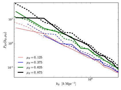
Figure 1: The comparison of the mean $\text{Lyman-}\alpha$ forest flux power spectrum between our prescription (solid) and the simulations in Ref. [45] (dashed) for four different $\mu_{S}$.

In figure 1 we compare the power spectrum of this prescription to the simulations in Ref. [45]. We find that on the scales of interest ($0.1\leq k_{S}\leq 1~{}h~{}{\rm Mpc}^{-1}$) the two power spectra are in reasonable agreement. Since we are taking logarithmic derivatives, these differences are unlikely to be very important.

In the following, we shall present the responses of the $\text{Lyman-}\alpha$ flux power spectrum to large-scale $\delta$ and $\eta$ in Section 3.1.1 and Section 3.1.2, respectively.

3.1.1 $\delta$ response

To simulate the $\text{Lyman-}\alpha$ forest power spectrum in overdense and underdense regions, or in the separate universe (SU), we set $\delta(z=2.5)=\pm 0.015$. To the leading order the response is independent of the choice of $\delta$, as long as $\delta\ll 1$. To avoid numerical errors, however, we set $\delta(z=2.5)$ to be large enough so that it is easy to extract the signal. Due to the presence of $\delta$, the cosmology in SUs is affected, and the new parameters are listed in table 1 of Ref. [27]. Since the SU simulations are meant to represent the overdense and underdense regions of the fiducial cosmology, there are a few rescalings we need to perform on the density field as we apply the FGPA prescription above, as well as on the $\text{Lyman-}\alpha$ forest flux power spectrum as we compute the response.

The first rescaling is the density fluctuation. Since the mean densities in SUs and the global universe are related by $\bar{\rho}_{\rm SU}=\bar{\rho}_{\rm G}\left(1+\delta\right)$, the mapping of the locally measured small-scale density fluctuation $\delta_{S}$ to the global universe at leading order is

$$\delta_{S}\rightarrow\delta_{S}(1+\delta)+\delta\,.$$ (3.5)

We then use the remapped $\delta_{S}$ for the FGPA prescription to compute the $\text{Lyman-}\alpha$ forest flux in SUs.

The second rescaling is the volume. To leading order, the scale factors in SUs and the global universe are related by $a_{\rm SU}=a_{\rm G}(1-\delta/3)$, with $\delta$ now normalized for the appropriate redshift matching in our simulations as described in the Appendix of Ref. [27]. We would like to compare the observables at the same physical time and coordinate. As the simulation box has the same comoving volume, the physical volume would be changed by a factor of $(1-\delta)$. The power spectrum is normalized by the volume, hence to compare the power spectrum in SUs with the one in the global universe we have to rescale it as

$$P_{FF}(k_{S},\mu_{S})\rightarrow(1+\delta)P_{FF}(k_{S},\mu_{S})\,.$$ (3.6)

We finally rescale the wavenumber of the power spectrum measured in SUs. The reason is identical to the volume rescaling: the power spectra in separate universes are quantified in their own comoving coordinate with different scale factors, so we need to rescale the wavenumbers to the comoving coordinate of the fiducial universe for a fair comparison. Since the wavenumber is proportional to the inverse of length, this results in a shift in the power spectrum as

$$P_{FF}(k_{S},\mu_{S})\rightarrow P_{FF}(k_{S},\mu_{S})\left[1+\frac{\delta}{3}\frac{d\ln P_{FF}(k_{S},\mu_{S})}{d\ln k_{S}}\right]\,.$$ (3.7)

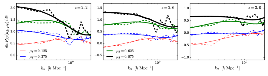
Figure 2: The responses of the $\text{Lyman-}\alpha$ forest flux power spectrum to the large-scale overdensity $\delta$. The left, middle and right panels show the response, $\partial\ln P_{FF}/\partial\delta$ at $z=2.2$, 2.6, and 3.0, respectively. The dashed lines are measurements of our SU simulations with $\delta(z=2.5)=\pm 0.015$, whereas the solid lines are smoothed by the Savitzky-Golay filter and then interpolated using the cubic spline (details are described in the main text). The thin to thick lines show the responses of different lines-of-sight with $\mu_{S}=0.125$, 0.375, 0.625, and 0.875.

We estimate the response of the $\text{Lyman-}\alpha$ forest flux power spectrum to $\delta$ as

$$\frac{\partial\ln P_{FF}(k_{S},\mu_{S})}{\partial\delta}=b^{FF}_{\delta}=\frac{P_{FF}(k_{S},\mu_{S}|\delta_{+})-P_{FF}(k_{S},\mu_{S}|\delta_{-})}{P_{FF}(k_{S},\mu_{S})}\frac{1}{\delta_{+}-\delta_{-}}\,.$$ (3.8)

The dashed lines in figure 2 show the measured $\partial\ln P_{FF}(k_{S},\mu_{S})/\partial\delta$ at $z=2.2$ (left), 2.6 (middle), and 3.0 (right) from our SU simulations. The thin to thick lines show the responses of different lines-of-sight with $\mu_{S}=0.125$, 0.375, 0.625, and 0.875. Since the measurements are noisy, we smooth them using the Savitzky-Golay filter [49] of window length 53 and poly order 8 and then apply the cubic spline to interpolate in $\ln k$-space. We visually inspect the smoothing, in particular at $0.1\leq k_{S}\leq 1~{}h~{}{\rm Mpc}^{-1}$, which is used for the Fisher matrix calculation in Section 4. Note that as the main purpose of this paper is to study the constraint on $f_{\rm NL}$, as long as the dependences of scale, angle, and redshift of the response to $\delta$ are different from that to $\phi$, the choice of smoothing should have relatively small impact on our result. We find a mild redshift evolution, with a slightly larger response at lower redshifts. We also find that on large scales ($k_{S}\lesssim 1~{}h~{}{\rm Mpc}^{-1}$) the response along the line-of-sight is larger than that in the transverse direction, which is most likely due to redshift-space distortions amplifying the effect. We shall use the solid lines (smoothed responses) for the Fisher forecast in Section 4.

3.1.2 $\eta$ response

Due to the peculiar velocities, the redshift- and real-space coordinates in the radial direction are related through $s=r+v_{\parallel}/(aH)$. In the presence of the large-scale velocity gradient, the redshift-space coordinate transforms further as $s\to s-r\eta$, which is effectively a stretching in the radial direction [27]. In order to conserve the total number of hydrogen atoms, the optical depth must therefore change by $(1-\eta)^{-1}$. In addition, due to this effective radial stretching we must also divide the thermal broadening parameter by $(1-\eta)$. We apply these changes in the FGPA prescription to compute the $\text{Lyman-}\alpha$ forest flux power spectrum, with $\eta=\pm 0.01$. Note that, as for $\delta$, the response is independent of the choice of $\eta$ at leading order.

We estimate the response of the $\text{Lyman-}\alpha$ forest flux power spectrum to $\eta$ as

$$\frac{\partial\ln P_{FF}(k_{S},\mu_{S})}{\partial\eta}=b^{FF}_{\eta}=\frac{P_{FF}(k_{S},\mu_{S}|\eta_{+})-P_{FF}(k_{S},\mu_{S}|\eta_{-})}{P_{FF}(k_{S},\mu_{S})}\frac{1}{\eta_{+}-\eta_{-}}\,.$$ (3.9)

The measurements of $d\ln P_{FF}(k_{S},\mu_{S})/d\eta$ from our SU simulations are shown as the dashed lines in figure 3. As for the response to $\delta$, we smooth the raw measurements from simulations. However, as the scale-dependences are different, for the response to $\eta$ we first smooth the measurements with Savitzky-Golay filter of window length 255 and poly order 29, and then apply the cubic spline to interpolate in $\ln k$-space. We also visually inspect the smoothing at the scale of interest, i.e. $0.1\leq k_{S}\leq 1~{}h~{}{\rm Mpc}^{-1}$. The results are shown as the solid lines. We find that similar to $d\ln P_{FF}(k_{S},\mu_{S})/d\delta$, $d\ln P_{FF}(k_{S},\mu_{S})/d\eta$ is larger at lower redshift. However, the response to $\eta$ has stronger evolution in $\mu_{S}$. This is likely due to the higher sensitivity of $P_{FF}(k_{S},\mu_{S})$ to $\eta$ than to $\delta$. The solid lines (smoothed responses) will also be used for the Fisher forecast in Section 4.

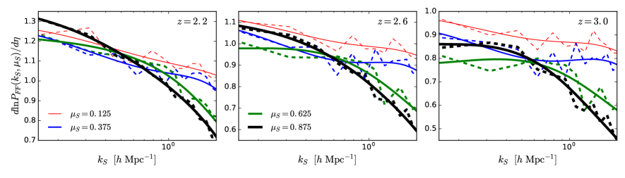
Figure 3: Same as figure 2, but for the responses of the $\text{Lyman-}\alpha$ forest flux power spectrum to the large-scale velocity gradient $\eta$, i.e. $\partial\ln P_{FF}/\partial\eta$.

3.2 Lyman-$\alpha$ forest flux power spectrum response to primordial non-Gaussianity

While the $\text{Lyman-}\alpha$ forest flux power spectrum responds to large-scale $\delta$ and $\eta$ due to the nonlinear gravitational evolution, or equivalently non-zero squeezed-limit bispectrum, in the presence of primordial non-Gaussianity it will also be modulated by $\phi$. Specifically, the local-type primordial non-Gaussianity changes $\sigma_{8}$ locally, and the $\text{Lyman-}\alpha$ forest flux power spectrum is affected accordingly. Following the formalism in Ref. [32], we can rewrite the derivative of $P_{FF}(k_{S},\mu_{S})$ with respect to $\phi$ into $\sigma_{8}$ as

$$b^{FF}_{\phi}=\frac{\partial\ln P_{FF}(k_{S},\mu_{S})}{\partial\phi}=\frac{\partial\ln P_{FF}(k_{S},\mu_{S})}{\partial\sigma_{8}}\frac{\partial\sigma_{8}}{\partial\phi}=2f_{\rm NL}\frac{\partial\ln P_{FF}(k_{S},\mu_{S})}{\partial\ln\sigma_{8}}\,.$$ (3.10)

In Ref. [45], a suite of simulations with different $\sigma_{8}$’s has been performed, and so it is ideal to study how the $\text{Lyman-}\alpha$ forest flux power spectrum responds to the primordial non-Gaussianity. Here we briefly describe the simulations and refer the readers to Ref. [45] for more details.

The cosmological parameters for the simulations are $\Omega_{m}=0.3$, $\Omega_{\Lambda}=0.7$, $\Omega_{b}=0.05$, $h=0.7$, and $n_{s}=1$. The three values for $\sigma_{8}$ are 0.6396, 0.7581, and 0.8778. The box size is $60~{}h^{-1}~{}{\rm Mpc}$ with $2\times 512^{3}$ particles (for dark matter and gas) and softening length of $4~{}h^{-1}~{}{\rm kpc}$. The initial conditions are set up by the Zel’dovich approximation at $z=49$, and the simulations are carried out by GADGET-2 [47]. The $\text{Lyman-}\alpha$ forest flux power spectrum is described by

$$P_{FF}(k_{S},\mu_{S})=(b^{F}_{\delta})^{2}(1+\beta_{F}\mu_{S}^{2})^{2}P_{l}(k_{S}){\mathcal{D}}_{\rm NL}(k_{S},\mu_{S})\,,$$ (3.11)

with the fitting formula accounting for the small-scale nonlinearity given by [45]

$${\mathcal{D}}_{\rm NL}(k,\mu)=\exp\left\{q_{1}\Delta^{2}(k)\left[1-\left(\frac{k}{k_{v}}\right)^{a_{v}}\mu^{b_{v}}\right]-\left(\frac{k}{k_{p}}\right)^{2}\right\}\,,\quad\Delta^{2}(k)=\frac{1}{2\pi^{2}}k^{3}P_{l}(k)\,,$$ (3.12)

where there are five fitting parameter $q_{1}$, $a_{v}$, $b_{v}$, $k_{v}$, and $k_{p}$. The values of the bias and the fitting parameters for different values of $\sigma_{8}$ can be found in table 8 and 9 of Ref. [45].

We can estimate the response of the $\text{Lyman-}\alpha$ forest flux power spectrum to $\sigma_{8}$ by

$$\frac{\partial\ln P_{FF}(k_{S},\mu_{S})}{\partial\ln\sigma_{8}}=\frac{\sigma_{8,0}}{P_{FF}(k_{S},\mu_{S}|\sigma_{8,0})}\frac{P_{FF}(k_{S},\mu_{S}|\sigma_{8,+})-P_{FF}(k_{S},\mu_{S}|\sigma_{8,-})}{\sigma_{8,+}-\sigma_{8,-}}\,,$$ (3.13)

where $\sigma_{8,(-,0,+)}$ refers to 0.6396, 0.7581, and 0.8778 respectively. Since Ref. [45] provides the fitting parameters as well as the bias parameters of the $\text{Lyman-}\alpha$ forest flux power spectrum for various redshifts and $\sigma_{8}$, we can thus numerically evaluate the response with eq. (3.13). Note, however, that in Ref. [45] the same mean flux is assumed for simulations with different $\sigma_{8}$’s. In reality, different $\sigma_{8}$ would result in different long-wavelength density perturbation. As the density fluctuation is nonlinearly related to the flux, i.e. through eq. (3.1), the large-scale mean flux would also be different for simulations with different $\sigma_{8}$. Lacking enough information to recover this effect, we ignore it in this paper but point out that taking this effect into account will boost up the signal of $f_{\rm NL}$. As a result, our estimated constraint on $f_{\rm NL}$ using the Fisher matrix is likely to be conservative.

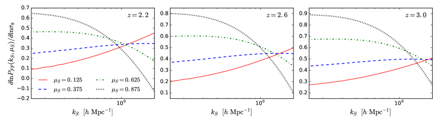
Figure 4: The responses of the $\text{Lyman-}\alpha$ forest flux power spectrum to $\sigma_{8}$ (or equivalently the local-type primordial non-Gaussianity with eq. (3.10)) at $z=2.2$ (left), 2.6 (middle), and 3.0 (right). The solid, dashed, dot-dashed, and dotted lines show the response at $\mu_{S}=0.125$, 0.375, 0.625, and 0.875, respectively.

The left, middle, and right panels of figure 4 show the response of the $\text{Lyman-}\alpha$ forest flux power spectrum to $\sigma_{8}$ at $z=2.2$, 2.6, and 3.0, respectively. Different line styles represent different lines-of-sight. We find that opposite to the large-scale $\delta$ and $\eta$, the $\text{Lyman-}\alpha$ forest flux power spectrum responds stronger to the local-type primordial non-Gaussianity at higher redshift. This trend is the same as the reduced matter squeezed-limit bispectrum with local $f_{\rm NL}$ (see e.g. figure 2.1 of Ref. [50]). Since the responses to gravitational evolution and primordial non-Gaussianity have different redshift dependences, using the data from multiple redshifts would help break the degeneracy between parameters and improve the constrains on $f_{\rm NL}$.

Another interesting but unfortunate fact is that while linear theory predicts a scale-independent response $d\ln P_{l}/d\ln\sigma_{8}=2$, simulations yield $d\ln P_{FF}(k_{S},\mu_{S})/d\ln\sigma_{8}<2$ on all scales and angles. This indicates that the signal of the primordial non-Gaussianity from the response of the $\text{Lyman-}\alpha$ forest flux power spectrum is smaller than that of the linear power spectrum. We find that on large scales ($k\lesssim 1~{}h~{}{\rm Mpc}^{-1}$) the cancellation is due to the Kaiser factor $(b^{F}_{\delta}+b^{F}_{\eta}f\mu_{S}^{2})^{2}$, and this cancellation is weaker along the line-of-sight. The fitting formula ${\mathcal{D}}_{\rm NL}(k_{S},\mu_{S})$ damps the response along the line-of-sight on small scales ($k\gtrsim 1~{}h~{}{\rm Mpc}^{-1}$), whereas it has negligible impact for the transverse direction on all scales.

A similar set of simulations has been performed in Ref. [26] with different amplitudes of primordial spectrum $A_{s}$. Using their fitting formula and parameters, we find a comparable result, i.e. the response is larger for line-of-sight direction on large scale, while on small scales the trend reverses, with the turning point at $\sim 1~{}h~{}{\rm Mpc}^{-1}$. The redshift dependence of the response is also similar. Given the similarity between the two sets of simulations, we use the more recent results for updated cosmological parameters as well as better simulation resolution. As the response to $\delta$ and $\eta$, the results shown in figure 4 will be used for the Fisher forecast in Section 4.

4 Expected constraint on primordial non-Gaussianity

One of the most exciting aspect of the large-scale structure is to constrain the local primordial non-Gaussianity, from which we can learn whether inflation is driven by one or multiple fields (see e.g. Ref. [51] for a review). Generally speaking, to acquire a competitive measurement of the squeezed-limit bispectrum from large-scale structure, one needs both a very large volume (to reach the squeezed limit), a sensitive probe (e.g. high galaxy number density for galaxy bispectrum), and systematic robustness, since the largest scales are typically the most contaminated in realistic large-scale structure surveys. The cross-correlation between the large-scale quasar density and small-scale $\text{Lyman-}\alpha$ forest flux power spectrum provides such an arena: (1) the current and future quasar surveys have huge volume; (2) the cross-correlation between these two tracers should be very clean. We will discuss this briefly in Section 5.

To explore the ability of constraining $f_{\rm NL}$ by cross-correlating the large-scale quasar density and small-scale $\text{Lyman-}\alpha$ forest flux power spectrum, we use the Fisher matrix (see e.g. Ref. [52] for a review) to forecast the constraint. Specifically, the Fisher matrix of $B_{FFq}^{\rm sq}(\mathbf{k}_{S},k_{L})$ is given by

$$F_{\alpha\beta}=\sum_{k_{S}=k_{S,\rm min}}^{k_{S,\rm max}}\sum_{\mu_{S}=0}^{1}\sum_{k_{L}=k_{L,\rm min}}^{k_{L,\rm max}}\frac{1}{\left[\Delta B_{FFq}^{\rm sq}(k_{S},\mu_{S},k_{L})\right]^{2}}\frac{\partial B^{\rm sq}_{FFq}(k_{S},\mu_{S},k_{L})}{\partial p_{\alpha}}\frac{\partial B^{\rm sq}_{FFq}(k_{S},\mu_{S},k_{L})}{\partial p_{\beta}}\,,$$ (4.1)

where $p_{\alpha}\in(b_{\delta}^{q},b_{\delta}^{F},b_{\eta}^{F},f_{\rm NL})$ are the parameters of interest. The constraint on $p_{\alpha}$ as well as the correlation between $p_{\alpha}$ and $p_{\beta}$ are then

$${\rm err}\left[p_{\alpha}\right]=\sqrt{\left(F^{-1}\right)_{\alpha\alpha}}\,,\quad{\rm corr}\left[p_{\alpha},p_{\beta}\right]=\frac{\left(F^{-1}\right)_{\alpha\beta}}{{\rm err}\left[p_{\alpha}\right]{\rm err}\left[p_{\beta}\right]}\,.$$ (4.2)

The signal of the squeezed-limit bispectrum is

$$B^{\rm sq}_{FFq}(\mathbf{k}_{S},k_{L})\> =P_{FF}(\mathbf{k}_{S})P_{l}(k_{L})\bigg{\{}\left[b^{q}_{\delta}+2f_{\rm NL}\delta_{c}\left(b^{q}_{\delta}-1\right)M^{-1}(k_{L})\right]\left[b^{FF}_{\delta}+\frac{f}{3}b^{FF}_{\eta}+M^{-1}(k_{L})b^{FF}_{\phi}\right]$$

$$\hskip 91.04872pt+\frac{f}{3}b^{FF}_{\delta}+\frac{f^{2}}{5}b^{FF}_{\eta}+\frac{f}{3}M^{-1}(k_{L})b^{FF}_{\phi}\bigg{\}}\,,$$ (4.3)

and we take the partial derivatives of the signal with respect to the four parameters with the equality that

$$\frac{\partial b^{FF}_{\phi}}{\partial f_{\rm NL}}=\frac{\partial}{\partial f_{\rm NL}}\left[2f_{\rm NL}\frac{\partial\ln P_{FF}(\mathbf{k}_{S})}{\partial\ln\sigma_{8}}\right]=2\frac{\partial\ln P_{FF}(\mathbf{k}_{S})}{\partial\ln\sigma_{8}}=\frac{b^{FF}_{\phi}}{f_{\rm NL}}\,.$$ (4.4)

For the error of the squeezed-limit bispectrum, we set $\Delta k=k_{F}$ and get

$$\left[\Delta B_{FFq}^{\rm sq}(k_{S},\mu_{S},k_{L})\right]^{2}=\frac{(2\pi)^{3}}{k_{F}^{3}}P_{FF,t}^{2}(\mathbf{k}_{S})P_{qq,t}(k_{L})\frac{k_{F}^{4}}{4\pi^{2}k_{S}^{2}k_{L}^{2}\Delta\mu_{S}}\,,$$ (4.5)

where the quasar power spectrum is

$$P_{qq}(k_{L})=\left[\left(b^{q}_{\delta}\right)^{2}+\frac{2}{3}fb^{q}_{\delta}+\frac{1}{5}f^{2}\right]P_{l}(k_{L})\,.$$ (4.6)

We follow Ref. [53] to compute the noise of the $\text{Lyman-}\alpha$ flux power spectrum that includes both the aliasing noise and actual spectrograph noise, whereas we assume that the noise of the quasar power spectrum is dominated by the Poisson shot noise $P_{qq,\rm noise}=V_{\rm survey}/N_{q}$ with $N_{q}$ being the number of quasars in the survey.

redshift	$V_{\rm survey}$ [$h^{-3}~{}{\rm Gpc}^{3}$]	$N_{q}/{\rm deg}^{2}/\Delta z$	$N_{q}$
2.0-2.2	11.42	19	266,000
2.2-2.4	11.53	16	224,000
2.4-2.6	11.55	12	168,000
2.6-2.8	11.51	8	112,000
2.8-3.0	11.41	5	70,000

Table 1: The survey parameters based on DESI for the Fisher forecast calculation.

As a concrete example, we utilize the survey parameters of DESI [54, 55] to numerically evaluate $F_{\alpha\beta}$. DESI will take spectra of quasars at $2\leq z\leq 3$ for $\text{Lyman-}\alpha$ forest absorption features across (at least) 14,000 square degrees, with the number density as a function of redshift given in figure 3.17 of Ref. [55]. In this paper we choose $\Delta z=0.2$, and so there are five redshift bins. The key survey parameters are summarized in table 1, with the volume computed assuming the fiducial cosmology in Ref. [45], i.e. flat $\Lambda$CDM with $\Omega_{m}=0.3$ and $\Omega_{b}=0.05$. We assume the quasar bias to be $b_{\delta}^{q}(z)=3.6D(z=2.4)/D(z)$ [56], where $D(z)$ is the linear growth. For the bias and fitting parameters of the $\text{Lyman-}\alpha$ forest flux power spectrum, we adopt the values in table 8 and 9 of Ref. [45]. We assume the fiducial $f_{\rm NL}$ to be zero, i.e. no primordial non-Gaussianity.

Since we are studying the constraining power for the squeezed-limit bispectrum consisting of small-scale $\text{Lyman-}\alpha$ forest flux power spectrum and large-scale quasar overdensity, we consider the range of scales to be $k_{F}\leq k_{L}\leq 0.05~{}h~{}{\rm Mpc}^{-1}$ and $0.1\leq k_{S}\leq 1~{}h~{}{\rm Mpc}^{-1}$, where the fundamental frequency $k_{F}=2\pi/V_{\rm survey}^{1/3}$ depends on the survey volume $V_{\rm survey}$ in various redshift bins. We consider four lines-of-sight for the $\text{Lyman-}\alpha$ forest flux power spectrum, i.e. $\Delta\mu_{S}=0.25$ for $\mu_{S}=0.125$, 0.375, 0.625, and 0.875 as the results shown in Section 3. The Fisher matrix is thus the summation of all scales, lines-of-sight, and redshifts for eq. (4.1).

For one redshift bin, there are three bias parameters ($b_{\delta}^{q}$, $b_{\delta}^{F}$, and $b_{\eta}^{F}$). Note that while we assume that the fiducial bias parameters at different redshifts are related by the linear growth, in the Fisher matrix we still conservatively treat them as independent parameters. In total there are 15 bias parameters, and so the Fisher matrix has the dimension of 16 including $f_{\rm NL}$.

Using the inverse Fisher matrix, we compute the 1-$\sigma$ constraints on the parameters as well as their correlation through eq. (4.2). We find ${\rm err}[f_{\rm NL}]=77$ from using the squeezed-limit bispectrum of the small-scale $\text{Lyman-}\alpha$ forest flux power spectrum and the large-scale quasar overdensity alone for DESI survey parameters. To better understand what dominates the constraint on $f_{\rm NL}$, we artificially set the noise of quasar and $\text{Lyman-}\alpha$ forest flux power spectrum to zero. In the absence of the shot noise of the quasar power spectrum, we obtain ${\rm err}[f_{\rm NL}]=46$, whereas in the absence of the noise of the $\text{Lyman-}\alpha$ forest flux power spectrum, we have ${\rm err}[f_{\rm NL}]=1.2$. In the absence of both quasar and $\text{Lyman-}\alpha$ forest flux noise, i.e. the sample variance limit, the constraint becomes ${\rm err}[f_{\rm NL}]=0.7$. It is thus clear that the noise of the $\text{Lyman-}\alpha$ forest flux power spectrum dominates the constraint on $f_{\rm NL}$. Specifically, we find that at $z=2.2$ the signal-to-noise ratio of the $\text{Lyman-}\alpha$ forest flux power spectrum per $k$ mode is of order $10^{-1}$ at $k_{S}=0.1~{}h~{}{\rm Mpc}^{-1}$ and $10^{-3}$ at $k_{S}=1~{}h~{}{\rm Mpc}^{-1}$. The signal-to-noise ratio is even smaller at higher redshift.

On top of the constraint on $f_{\rm NL}$, we also find that the constraints on the biases are poor due to the high degeneracy: the typical absolute values of cross-correlation coefficients between $b_{\delta}^{q}$, $b_{\delta}^{F}$, and $b_{\eta}^{F}$ in one redshift bin are all greater than 0.99. This is because only the three-point function is used to constrain the parameters. To break the degeneracy between biases, we add both the quasar and $\text{Lyman-}\alpha$ forest flux power spectra into the Fisher calculation to constrain $b_{\delta}^{q}$, $b_{\delta}^{F}$, and $b_{\eta}^{F}$ (but not $f_{\rm NL}$). We use the same scales for the power spectra as for the squeezed-limit bispectrum, and assume no covariance between the three measurements. We find that including the power spectra largely reduces the correlation between $b_{\delta}^{q}(z)$ and $(b_{\delta}^{F},b_{\eta}^{F})$; $b_{\delta}^{F}$ and $b_{\eta}^{F}$ are still highly anti-correlated due to the lack of lines-of-sight. Most interestingly, breaking the degeneracy between biases also improves the constraint on $f_{\rm NL}$ by 30%, to ${\rm err}[f_{\rm NL}]=56$.

In principle, there is also signal for $f_{\rm NL}$ from the quasar scale-dependent bias, i.e. in $b^{q}_{\phi}$. If this is included in the Fisher analysis, we obtain ${\rm err}[f_{\rm NL}]=4.6$, which indicates that the constraint on $f_{\rm NL}$ is dominated by the quasar scale-dependent bias. This is due to the low signal-to-noise ratio of the quasar-$\text{Lyman-}\alpha$ forest squeezed-limit bispectrum, compared to the quasar scale-dependent bias. Note that the advantage of the cross-correlation is that the signal suffers less observational systematics than the auto-correlation, and so the result is generally cleaner. Moreover, since different observables suffer different systematics, it is useful to constrain $f_{\rm NL}$ using multiple measurements to confirm the result.

We would like to caution the readers that some astrophysical effects are neglected in our calculation. For example, due to the clustering of galaxies and quasars, on scales larger than the mean-free-path of the ionizing photons ($\sim 350$ Mpc) the UV background is not uniform, and so the ionization equilibrium in regions with greater separations would depend on the density of the local regions [57]. This introduces two new bias parameters $b_{\Gamma}^{F}$ and $b_{\Gamma}^{FF}$ which correspond to the response of the mean flux and power spectrum to fluctuations in the photoionization background. The actual calculation of the cross-correlation between the $\text{Lyman-}\alpha$ forest flux power spectrum and the large-scale UV fluctuation is beyond the scope of this paper. However, we expect that such an effect would have different scale-dependences compared to the squeezed-limit bispectrum due to local primordial non-Gaussianity, therefore if the effect is correctly modeled then the constraint on $f_{\rm NL}$ should not be biased or degrade, as for the constraint on dark energy using BAO from $\text{Lyman-}\alpha$ forest flux power spectrum [58].

5 Conclusions

In this paper, we show that the squeezed-limit bispectrum $B_{YYX}^{\rm sq}$, where $Y$ is the small-scale modes and $X$ the large-scale mode, can be computed as the response of the small-scale power spectrum $P_{YY}$ to the large-scale $\delta_{X}$ fluctuation. This is similar to the position-dependent power spectrum in which one measures the correlation between $P_{YY}$ and $\delta_{X}$ [33]. Using the small-scale $\text{Lyman-}\alpha$ forest flux power spectrum and the large-scale quasar overdensity as an example, we predict their squeezed-limit bispectrum to be the responses to the large-scale density fluctuation $\delta$, the large-scale velocity gradient $\eta$, and the local-type primordial non-Gaussianity $\phi$.

Since the responses of the $\text{Lyman-}\alpha$ forest flux power spectrum are highly nonlinear, we measure them from separate universe simulations. Specifically, a long-wavelength $\delta$ can be equivalently understood as modifying the local cosmology, and we can directly simulate the structure formation in such an environment by adjusting the local cosmological parameters. In the presence of $\eta$, the redshift-space coordinate is stretched in the radial direction, and we thus rescale the small-scale $\text{Lyman-}\alpha$ forest flux power spectrum in the line-of-sight direction. Finally, in the presence of local primordial non-Gaussianity, the local $\sigma_{8}$ is modulated by the primordial potential $\phi$, and we apply the fitting formula and parameters in Ref. [45] to model the small-scale $\text{Lyman-}\alpha$ forest flux power spectrum with different $\sigma_{8}$. The response of the small-scale $\text{Lyman-}\alpha$ forest flux power spectrum to the large-scale fluctuations can thus be estimated by taking numerical derivatives with respect to $\delta$, $\eta$, and $\phi$. With the responses measured from the separate universe simulations, we can thus numerically evaluate the squeezed-limit bispectrum of the $\text{Lyman-}\alpha$ forest flux power spectrum and quasar overdensity (see Ref. [59] for the squeezed-limit bispectrum where the responses of the small-scale power spectrum to the large-scale fluctuations can be computed perturbatively and analytically).

We then explore the constraining power of the local primordial non-Gaussianity $f_{\rm NL}$ with the squeezed-limit bispectrum of $\text{Lyman-}\alpha$ forest flux power spectrum and quasar overdensity. We apply the response approach to predict the signal of the bispectrum and the Fisher matrix to test the observability of $f_{\rm NL}$. In principle, this measurement should be systematically very clean: the selection function, reddening, point spread function, and similar effects that plague galaxy surveys at large scales and so contaminate quasar catalogs will not systematically correlate with measurements of the small-scale $\text{Lyman-}\alpha$ forest flux power spectrum. If fewer quasars are detected, this does not affect the measurements of the small-scale power spectrum in the forest, but only its noise. Similarly, effects that are slowly varying with observed frequency (reddening, loosing of photons due to point spread function smearing, etc) are not affecting the size of small-scale fluctuations relative to the mean. This makes this measurements considerably more appealing than, for example, the quasar auto-bispectrum. On the other hand, there are astrophysical systematics that could enter, via other, non-gravitational sources of large-scale fluctuations in the Universe, such as those arising from photoionization rate and temperature fluctuations [57]. But these must still respect physical constraints which results in different scale dependencies (on sufficiently large scales) that can be isolated and separated from primordial non-Gaussianity.

We find that for DESI the expected constraint is ${\rm err}[f_{\rm NL}]\sim 80$ using the squeezed-limit bispectrum alone, and the result is dominated by the error of the $\text{Lyman-}\alpha$ forest flux power spectrum. If we include both the quasar and $\text{Lyman-}\alpha$ forest flux power spectra to break the degeneracy between biases, the constraint on $f_{\rm NL}$ improves to ${\rm err}[f_{\rm NL}]\sim 60$. Note that while the effect of the large-scale tidal field is neglected, we do not expect the constraint on $f_{\rm NL}$ to worsen much if the tidal field is included, as it has different dependences on scale and angle from the local primordial non-Gaussianity, and so the degeneracy should be weak. Similar argument applies to other astrophysical effects that may be ignored in our calculation. However, we note that our derivatives with respect to $\sigma_{8}$ variation are calculated at a fixed mean flux, since the authors of Ref. [45] do not provide sufficient information to correct for their renormalization of flux. While this underestimates the real effect, we also know that the continuum fitting procedure typically results in the power spectrum being measured around the local value of the mean flux. This subtlety might affect our sensitivity estimate, but is unlikely to be dominant.

While we use the $\text{Lyman-}\alpha$ forest flux forest power spectrum and the quasar overdensity as a concrete example to predict their squeezed-limit bispectrum using the response approach, this approach can be applied to other observables to forecast the signal of the squeezed-limit bispectrum. Especially, the separate universe simulations are very powerful to estimate the responses of the small-scale structure formation to the large-scale fluctuations, the response approach is thus useful to compute the squeezed-limit bispectrum of various observables for future observations.

Another application for our $\text{Lyman-}\alpha$ forest flux power spectrum response calculation is to compare with the measurement of the cross-correlation between CMB lensing and $\text{Lyman-}\alpha$ forest flux power spectrum recently presented in Ref. [37]. In that work, a cross-correlation is done in real space, between the CMB lensing convergence field $\kappa$ and the local measurements of the power spectrum. The authors quantify their results in terms of the effective $b_{2}^{\rm eff}$ parameter, which encodes the excess of the $\text{Lyman-}\alpha$ flux power spectrum response with respect to that of the linear field. Since in our simulations, the flux power spectrum response is always lower than that of the linear field, for all scales and lines-of-sight, this would imply $b_{2}^{\rm eff}<0$, while Ref. [37] find $b_{2}^{\rm eff}=1.16\pm 0.53$. There are many reasons for this discrepancy that could include a surprisingly large inaccuracies in our simulations or more likely the presence of unaccounted physical effects, such as damped $\text{Lyman-}\alpha$ systems or temperature or photoionization rate fluctuations. Since the presented measurement is a configuration-space measurement evaluated at zero separation, it is also possible that our approximation of a squeezed limit breaks down (i.e. there is significant contribution from other triangles). We leave a detailed comparison with this measurement for future work.

References

- [1] P. Creminelli, J. Noreña, M. Simonović and F. Vernizzi, Single-Field Consistency Relations of Large Scale Structure, JCAP 1312 (2013) 025, [1309.3557].
- [2] M. Peloso and M. Pietroni, Galilean invariance and the consistency relation for the nonlinear squeezed bispectrum of large scale structure, JCAP 1305 (2013) 031, [1302.0223].
- [3] L. Dai, E. Pajer and F. Schmidt, On Separate Universes, JCAP 1510 (2015) 059, [1504.00351].
- [4] W. Hu, C.-T. Chiang, Y. Li and M. LoVerde, Separating the Universe into real and fake energy densities, Phys. Rev. D94 (2016) 023002, [1605.01412].
- [5] W. Hu and A. Joyce, Separate Universes beyond General Relativity, 1612.02454.
- [6] B. Little, D. H. Weinberg and C. Park, Primordial fluctuations and nonlinear structure, Mon. Not. Roy. Astron. Soc. 253 (1991) 295–306.
- [7] A. L. Melott and S. F. Shandarin, Controlled experiments in cosmological gravitational clustering, Astrophys. J. 410 (1993) 469–481.
- [8] S. Shandarin, S. Habib and K. Heitmann, Origin of the Cosmic Network: Nature vs Nurture, Phys. Rev. D81 (2010) 103006, [0912.4471].
- [9] M. D. Schneider, S. Cole, C. S. Frenk and I. Szapudi, Fast generation of ensembles of cosmological N-body simulations via mode-resampling, Astrophys. J. 737 (2011) 11, [1103.2767].
- [10] J. Einasto, I. Suhhonenko, G. Hutsi, E. Saar, M. Einasto, L. J. Liivamagi et al., Towards understanding the structure of voids in the cosmic web, Astron. Astrophys. 534 (2011) A128, [1105.2464].
- [11] A. Pontzen, A. Slosar, N. Roth and H. V. Peiris, Inverted initial conditions: exploring the growth of cosmic structure and voids, Phys. Rev. D93 (2016) 103519, [1511.04090].
- [12] D. J. Eisenstein, H.-j. Seo, E. Sirko and D. Spergel, Improving Cosmological Distance Measurements by Reconstruction of the Baryon Acoustic Peak, Astrophys. J. 664 (2007) 675–679, [astro-ph/0604362].
- [13] N. Padmanabhan, X. Xu, D. J. Eisenstein, R. Scalzo, A. J. Cuesta, K. T. Mehta et al., A 2 per cent distance to =0.35 by reconstructing baryon acoustic oscillations - I. Methods and application to the Sloan Digital Sky Survey, Mon. Not. Roy. Astron. Soc. 427 (2012) 2132–2145, [1202.0090].
- [14] M. Takada and W. Hu, Power Spectrum Super-Sample Covariance, Phys. Rev. D87 (2013) 123504, [1302.6994].
- [15] Y. Li, W. Hu and M. Takada, Super-Sample Signal, Phys. Rev. D90 (2014) 103530, [1408.1081].
- [16] Y. Li, W. Hu and M. Takada, Super-Sample Covariance in Simulations, Phys. Rev. D89 (2014) 083519, [1401.0385].
- [17] K. Akitsu, M. Takada and Y. Li, Super-Survey Tidal Effect on Redshift-space Power Spectrum, 1611.04723.
- [18] E. Sirko, Initial conditions to cosmological N-body simulations, or how to run an ensemble of simulations, Astrophys. J. 634 (2005) 728–743, [astro-ph/0503106].
- [19] N. Y. Gnedin, A. V. Kravtsov and D. H. Rudd, Implementing the DC Mode in Cosmological Simulations with Supercomoving Variables, Astrophys. J. Suppl. 194 (2011) 46, [1104.1428].
- [20] C. Wagner, F. Schmidt, C.-T. Chiang and E. Komatsu, Separate Universe Simulations, Mon. Not. Roy. Astron. Soc. 448 (2015) L11–L15, [1409.6294].
- [21] C. Wagner, F. Schmidt, C.-T. Chiang and E. Komatsu, The angle-averaged squeezed limit of nonlinear matter N-point functions, JCAP 1508 (2015) 042, [1503.03487].
- [22] T. Lazeyras, C. Wagner, T. Baldauf and F. Schmidt, Precision measurement of the local bias of dark matter halos, JCAP 1602 (2016) 018, [1511.01096].
- [23] Y. Li, W. Hu and M. Takada, Separate Universe Consistency Relation and Calibration of Halo Bias, Phys. Rev. D93 (2016) 063507, [1511.01454].
- [24] T. Baldauf, U. Seljak, L. Senatore and M. Zaldarriaga, Linear response to long wavelength fluctuations using curvature simulations, 1511.01465.
- [25] V. Desjacques, D. Jeong and F. Schmidt, Large-Scale Galaxy Bias, 1611.09787.
- [26] P. McDonald, Toward a measurement of the cosmological geometry at Z 2: predicting lyman-alpha forest correlation in three dimensions, and the potential of future data sets, Astrophys. J. 585 (2003) 34–51, [astro-ph/0108064].
- [27] A. M. Cieplak and A. Slosar, Towards physics responsible for large-scale Lyman-alpha forest bias parameters, JCAP 1603 (2016) 016, [1509.07875].
- [28] C.-T. Chiang, Y. Li, W. Hu and M. LoVerde, Quintessential Scale Dependence from Separate Universe Simulations, 1609.01701.
- [29] D. K. Hazra and T. G. Sarkar, Primordial Non-Gaussianity in the Forest: 3D Bispectrum of Ly-alpha Flux Spectra Along Multiple Lines of Sight, Phys. Rev. Lett. 109 (2012) 121301, [1205.2790].
- [30] N. Kaiser, Clustering in real space and in redshift space, Mon. Not. Roy. Astron. Soc. 227 (1987) 1–27.
- [31] E. Komatsu and D. N. Spergel, Acoustic signatures in the primary microwave background bispectrum, Phys. Rev. D63 (2001) 063002, [astro-ph/0005036].
- [32] A. Slosar, C. Hirata, U. Seljak, S. Ho and N. Padmanabhan, Constraints on local primordial non-Gaussianity from large scale structure, JCAP 0808 (2008) 031, [0805.3580].
- [33] C.-T. Chiang, C. Wagner, F. Schmidt and E. Komatsu, Position-dependent power spectrum of the large-scale structure: a novel method to measure the squeezed-limit bispectrum, JCAP 1405 (2014) 048, [1403.3411].
- [34] H. Y. Ip and F. Schmidt, Large-Scale Tides in General Relativity, 1610.01059.
- [35] A. Barreira and F. Schmidt, Responses in Large-Scale Structure, ArXiv e-prints (Mar., 2017) , [1703.09212].
- [36] C.-T. Chiang, C. Wagner, A. G. Sánchez, F. Schmidt and E. Komatsu, Position-dependent correlation function from the SDSS-III Baryon Oscillation Spectroscopic Survey Data Release 10 CMASS Sample, JCAP 1509 (2015) 028, [1504.03322].
- [37] C. Doux, E. Schaan, E. Aubourg, K. Ganga, K.-G. Lee, D. N. Spergel et al., First detection of cosmic microwave background lensing and Lyman- forest bispectrum, Phys. Rev. D94 (2016) 103506, [1607.03625].
- [38] R. Scoccimarro, S. Colombi, J. N. Fry, J. A. Frieman, E. Hivon and A. Melott, Nonlinear evolution of the bispectrum of cosmological perturbations, Astrophys. J. 496 (1998) 586, [astro-ph/9704075].
- [39] E. Sefusatti and E. Komatsu, The bispectrum of galaxies from high-redshift galaxy surveys: Primordial non-Gaussianity and non-linear galaxy bias, Phys. Rev. D76 (2007) 083004, [0705.0343].
- [40] D. Jeong and E. Komatsu, Perturbation Theory Reloaded II: Non-linear Bias, Baryon Acoustic Oscillations and Millennium Simulation In Real Space, Astrophys. J. 691 (2009) 569–595, [0805.2632].
- [41] T. Baldauf, U. Seljak and L. Senatore, Primordial non-Gaussianity in the Bispectrum of the Halo Density Field, JCAP 1104 (2011) 006, [1011.1513].
- [42] M. Tellarini, A. J. Ross, G. Tasinato and D. Wands, Galaxy bispectrum, primordial non-Gaussianity and redshift space distortions, JCAP 1606 (2016) 014, [1603.06814].
- [43] N. Dalal, O. Dore, D. Huterer and A. Shirokov, The imprints of primordial non-gaussianities on large-scale structure: scale dependent bias and abundance of virialized objects, Phys. Rev. D77 (2008) 123514, [0710.4560].
- [44] S. Matarrese and L. Verde, The effect of primordial non-Gaussianity on halo bias, Astrophys. J. 677 (2008) L77–L80, [0801.4826].
- [45] A. Arinyo-i Prats, J. Miralda-Escudé, M. Viel and R. Cen, The Non-Linear Power Spectrum of the Lyman Alpha Forest, JCAP 1512 (2015) 017, [1506.04519].
- [46] M. LoVerde, S. Marnerides, L. Hui, B. Menard, A. Lidz, S. Marnerides et al., Gravitational Lensing as Signal and Noise in Lyman-alpha Forest Measurements, Phys. Rev. D82 (2010) 103507, [1004.1165].
- [47] V. Springel, The Cosmological simulation code GADGET-2, Mon. Not. Roy. Astron. Soc. 364 (2005) 1105–1134, [astro-ph/0505010].
- [48] F. Haardt and P. Madau, Radiative transfer in a clumpy Universe. 2. The Ultraviolet extragalactic background, Astrophys. J. 461 (1996) 20, [astro-ph/9509093].
- [49] W. H. Press, S. A. Teukolsky, W. T. Vetterling and B. P. Flannery, Numerical Recipes 3rd Edition: The Art of Scientific Computing. Cambridge University Press, New York, NY, USA, 3 ed., 2007.
- [50] C.-T. Chiang, Position-dependent power spectrum: a new observable in the large-scale structure. PhD thesis, Munich U., 2015. 1508.03256.
- [51] M. Alvarez et al., Testing Inflation with Large Scale Structure: Connecting Hopes with Reality, 1412.4671.
- [52] M. Tegmark, A. Taylor and A. Heavens, Karhunen-Loeve eigenvalue problems in cosmology: How should we tackle large data sets?, Astrophys. J. 480 (1997) 22, [astro-ph/9603021].
- [53] P. McDonald and D. Eisenstein, Dark energy and curvature from a future baryonic acoustic oscillation survey using the Lyman-alpha forest, Phys. Rev. D76 (2007) 063009, [astro-ph/0607122].
- [54] DESI collaboration, M. Levi et al., The DESI Experiment, a whitepaper for Snowmass 2013, 1308.0847.
- [55] DESI collaboration, A. Aghamousa et al., The DESI Experiment Part I: Science,Targeting, and Survey Design, 1611.00036.
- [56] A. Font-Ribera et al., The large-scale Quasar-Lyman alpha Forest Cross-Correlation from BOSS, JCAP 1305 (2013) 018, [1303.1937].
- [57] A. Pontzen, Scale-dependent bias in the baryonic-acoustic-oscillation-scale intergalactic neutral hydrogen, Phys. Rev. D89 (2014) 083010, [1402.0506].
- [58] A. Pontzen, S. Bird, H. Peiris and L. Verde, Constraints on ionising photon production from the large-scale Lyman-alpha forest, Astrophys. J. 792 (2014) L34, [1407.6367].
- [59] C.-T. Chiang, The halo squeezed-limit bispectrum with primordial non-Gaussianity: a power spectrum response approach, 1701.03374.