Large-deviations for spatial diffusion of cold atoms

Abstract

Large-deviations theory deals with tails of probability distributions and the rare events of random processes, for example spreading packets of particles. Mathematically, it concerns the exponential fall-of of the density of thin-tailed systems. Here we investigate the spatial density ${P_{t}(x)}$ of laser cooled atoms, where at intermediate length scales the shape is fat-tailed. We focus on the rare events beyond this range, which dominate important statistical properties of the system. Through a novel friction mechanism induced by the laser fields, the density is explored with the recently proposed nonnormalized infinite-covariant density approach. The small and large fluctuations give rise to a bi-fractal nature of the spreading packet.

In diffusion processes such as Brownian motion, the concentration of particles starting at the origin spreads out like a Gaussian, which is fully characterized by the mean squared-displacement. This is the result of the widely applicable Gaussian central limit theorem (CLT) Gardiner [2009]. Of no less importance is large-deviations theory Touchette [2009], which deals with the rare fluctuations of processes such as simple coin tossing random walks (see e.g., Ellis [1999]), extreme variations of the surface height in the Kardar-Parisi-Zhang model Krapivsky et al. [2014] and the tails of the position distribution in single-file diffusion  Meerson et al. [2016]; Hegde et al. [2014]. Mathematically, a prerequisite of the theory is that the cumulant generating function be “well behaved”, i.e. smooth and differentiable. Large-deviations theory works when the decay of the probability of the observable of interest is exponential (see details in Touchette [2009]). However many systems do not meet this requirement Touchette [2009], for example Lévy fat-tailed processes Bouchaud and Georges [1990]; Klafter et al. [1996]; Zaburdaev et al. [2015], where the decay rate is a power-law.

This is the case for a cloud of atoms undergoing Sisyphus laser-cooling  Cohen-Tannoudji and Phillips [1990], where both theoretically Marksteiner et al. [1996]; Kessler and Barkai [2012] and experimentally Sagi et al. [2012], it was shown that the central part of the spreading particle packet is described by the Lévy CLT Klafter and Sokolov [2011]. The latter deals with the sum of independent identically-distributed random variables, but unlike the classical Gaussian CLT, here the summands’ own distribution is heavy-tailed. As a result, Lévy’s CLT yields an infinite mean squared-displacement for the sum Klafter and Sokolov [2011], and consequently also the second cumulant. Large-deviations theory mainly deals with thin-tailed processes where extreme events are rare, but in Lévy processes these large fluctuations are dominant. To study the fluctuations in this system, we will show that the relevant tool is the asymptotic moment-generating function, which yields an infinite-covariant density (ICD) Kessler and Barkai [2012]; Rebenshtok et al. [2014a]. We will discuss the generality of this approach and its results below.

In an experimental situation, diverging moments are unphysical. For example, although the experiment in Sagi et al. [2012] shows a nice fit of the particles’ density to a symmetric Lévy distribution, clearly at finite times no particles traveling at finite velocities can ever be found infinitely far from their origin. The finiteness of all the moments requires that the power-law tail of the distribution be cut-off beyond some point. A full characterization of the system demands that this far asymptotic regime be captured correctly, as well as the intermediate asymptotic power-law of the Lévy CLT.

Model. Sisyphus cooling is controlled by two competing mechanism: the slow decay in time of large momenta due to an anomalous friction force that weakens at large velocities, and random momentum fluctuations which lead to heating Dalibard and Cohen-Tannoudji [1989]; Cohen-Tannoudji and Phillips [1990]. Within the framework of the semiclassical approximation, the trajectory of an atom which starts at the origin ${x(0)=0}$, with ${v(0)=0}$, is determined by the Langevin equations Marksteiner et al. [1996] (see supplementary material (SM) for a more in-depth review):

$${\dot{v}(t)=\mathcal{F}(v)+\sqrt{2D}\Gamma{(t)},\quad\quad\quad\dot{x}(t)=v(t),}$$ (1)

where ${\mathcal{F}(v)=-v/(1+v^{2})}$ is the deterministic cooling force, in dimensionless units Kessler and Barkai [2010] (physical units in SM). Asymptotically, ${\mathcal{F}(v)\sim-v}$ when ${v\ll 1}$ and ${\sim-1/v}$ when ${v\gg 1}$. ${\Gamma(t)}$ is a Gaussian white-noise with zero mean and ${\langle\Gamma(t)\Gamma(t^{\prime})\rangle=\delta(t-t^{\prime})}$. ${D=cE_{R}/{U}_{0}}$, where ${{U}_{0}}$ is the depth of the optical lattice, ${E_{R}}$ is the recoil energy and ${c\approx 20}$ is a constant whose precise value is specific to the type of atoms used in the experiment Cohen-Tannoudji and Phillips [1990]; Marksteiner et al. [1996]. ${U_{0}}$, and hence ${D}$, may be tuned in the lab, and are the control parameters of the system. Several anomalous statistical predictions of this model, Eq. (1), both in and out of equilibrium, were confirmed in experiments (see e.g., Douglas et al. [2006]; Katori et al. [1997]; Sagi et al. [2012]).

We wish to study the large deviations of the probability density function (PDF) of the particles’ positions, ${P_{t}(x)}$ at time ${t}$. Its Fourier-transform, ${\int_{-\infty}^{\infty}\exp(ikx)P_{t}(x){\rm{d}}x}$, from ${x\rightarrow k}$, is the moment-generating function Klafter and Sokolov [2011]

$${\hat{P}_{t}(k)=1+\sum_{m=1}^{\infty}\frac{(ik)^{2m}}{(2m)!}\langle{x^{2m}}(t)\rangle.}$$ (2)

The strategy we will employ is to derive the moments of the process, ${\langle x^{2m}(t)\rangle}$, for ${m=1,2,...}$ (odd moments are zero by symmetry), perform the summation in Eq. (2) and invert this function to obtain the density in ${x}$ space. Naively, we would expect a normalized density to emerge, but this, as we will show, appears not to be the case.

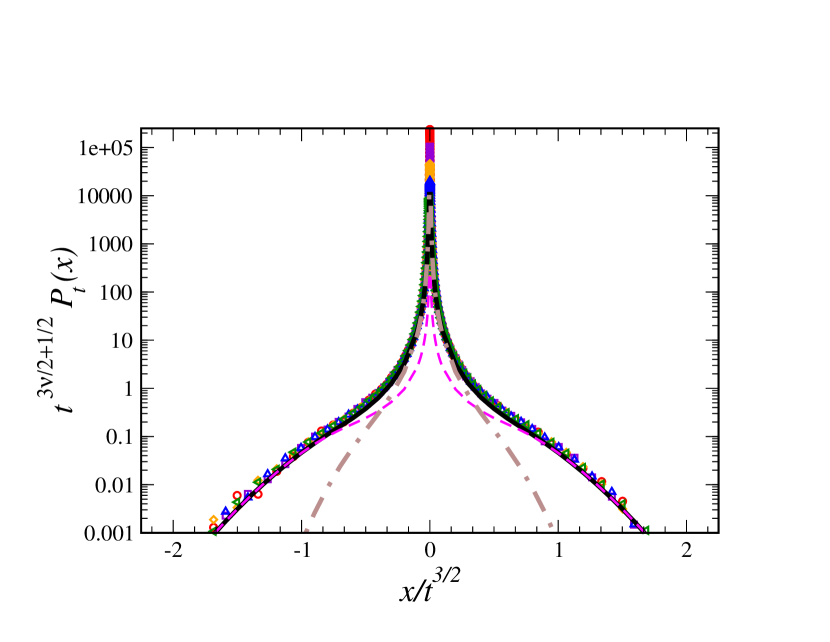
Figure 1: (Color online) Convergence of the particles position density in Sisyphus cooling, with $D=0.4$ (${\nu=7/6}$), to the form of the ICD, Eq. (12). Langevin simulation results Note [1] for $t=1000$ are represented by (green, left triangles), $t=1778$ (blue, up triangles), $t=3162$ (orange, diamonds), $t=5623$ (purple, squares) and $t=10000$ (red circles). The scaling limit function ${\mathcal{I}(z)}$, based on the areal PDFs of the Bessel excursion and the meander, is presented in (solid black line). Asymptotic theory for ${(x/t^{3/2})\ll 1}$ (dot-dashed brown line) and ${(x/t^{3/2})\gg 1}$ (magenta dashed line), correspond to Eqs. (10) and (11) respectively. Notice how ${\mathcal{I}(z)}$ diverges as ${x/t^{3/2}\rightarrow 0}$, and it is not integrable at this pole.

Scaling arguments for a nonnormalizable state. An initial insight into the position distribution, ${P_{t}(x)}$, may be gained as follows: Let ${W_{t}(x,v)}$ be the phase space distribution of the diffusive particle packet, at time ${t}$. Since for large ${v}$ the friction vanishes from Eq. (1), in this case we expect a scaling ${v\propto t^{1/2}}$. By integration over time, this implies ${x\propto t^{3/2}}$. Based on these scaling arguments we may write ${W_{t}(x,v)\sim t^{\xi}f\left(x/t^{3/2},v/t^{1/2}\right)}$. To determine the exponent ${\xi}$ we may use a simple argument (though it can be derived also rigorously): We note that when ${D<1}$ the marginal velocity equilibrium density is Douglas et al. [2006]; Lutz [2004]; Kessler and Barkai [2010]; Holz et al. [2015]; Dechant et al. [2016]

$${\lim_{t\rightarrow\infty}\mathbf{P}_{t}(v)\rightarrow\mathbf{P}_{eq}(v)\sim|v|^{-1/D},\quad(\mbox{when}\quad v\gg 1).}$$ (3)

The range ${D>1}$ is a heating phase, where an equilibrium state does not exist, hence we leave it out of the context of this work. By definition, this velocity density is related to the phase space distribution via

$${\mathbf{P}_{eq}(v)=\lim_{t\rightarrow\infty}t^{\zeta+3/2}\int_{-\infty}^{\infty}f\left(\frac{x}{t^{3/2}},\frac{v}{t^{1/2}}\right){\rm{d}}\left(\frac{x}{t^{3/2}}\right),}$$ (4)

hence from Eqs. (3,4) we find ${\zeta=-3/2-1/(2D)}$.

Using this result, integration of the scaling solution over velocity yields $P_{t}(x)\sim\mathcal{I}(z)/t^{1+1/(2D)}$ where $z=x/t^{3/2}$. This suggests, and indeed our rigorous theory shows, that there exists a limit such that

$${\mathcal{I}(z)=\lim_{t\rightarrow\infty}t^{1+1/(2D)}P_{t}(x).}$$ (5)

This limit is interesting since if we integrate Eq. (5) over $dz=dx/t^{3/2}$ we get from the normalization of $P_{t}(x)$, that the integral $\int_{-\infty}^{\infty}\mathcal{I}(z){\rm{d}}z\rightarrow\infty$. It follows that $\mathcal{I}(z)$ is not a normalized density, but rather a scaling solution that captures the non-unifrom convergence of the packet of particles. As we discuss below this scaling limit is not unique, but luckily there exists only one more scaling limit to the problem, and that is described by the well known Lévy CLT. In that sense the nonnormalised state ${\mathcal{I}(z)}$, being a limiting solution, is complementary to the CLT. In Fig. 1, we present simulation data from the cold atoms system with ${D=0.4}$ , which shows nice convergence with increasing time to the theory.

Excursions to untangle Langevin dynamics. The derivation of our main results uses a connection between the properties of constrained stochastic paths and Langevin dynamics, established in Marksteiner et al. [1996]; Barkai et al. [2014]. Let the times ${t_{1},t_{2},...t_{n}}$ denote the zero crossings of the stochastic process ${v(t)}$, Eq. (1). The time intervals between the crossing events, ${\tau_{1}=t_{1}-0,...\tau_{n}=t_{n}-t_{n-1}}$, are independent identically-distributed random variables, a property which is due to the Markovian Langevin process under investigation. The total measurement time is ${t=\sum_{i=1}^{n}\tau_{i}+\tau^{*}}$, where ${\tau^{*}}$ is the duration of the last interval, in which the velocity does not return to zero. The displacement accumulated by the particle during each interval is ${\chi_{i}=\int_{t_{i-1}}^{t_{i-1}+\tau_{i}}v(t){\rm{d}}t}$ (for the last step, ${\chi^{*}=\int_{t-\tau^{*}}^{t}v(t){\rm{d}}t}$), and the final random position of the particle at time ${t}$ is given by the sum ${x(t)=\sum_{i=1}^{n}{\chi_{i}}+\chi^{*}}$. Note that in this construction, the velocity path in all but the last interval starts and ends at zero, and is strictly positive or negative in between, hence the ${\tau_{i}}$s are determined by the first-passage time (to the velocity origin) distribution: ${g(\tau)\approx g^{*}\tau^{-3/2-1/(2D)},}$ for large ${\tau}$ Kessler and Barkai [2010]; Barkai et al. [2014]. The slow decaying power-law tail of this function, means that the duration of the last step might be as long as the sum of all the prior ones and it cannot be neglected. This is clearly a consequence of the weak friction at large velocities, that allows for very long flights without velocity zero crossings.

Each segment of the path ${v(t)}$, prior to the last, (i.e. between zero crossings), is approximated by a Bessel excursion in velocity space Barkai et al. [2014]; Kessler et al. [2014] (see Fig. 2). An excursion in the time interval ${[0,\tau_{i}]}$, is a stochastic trajectory which is constrained to begin close to the velocity origin, at ${v(0)=\epsilon\rightarrow 0}$, end at ${v(\tau_{i})=0}$, and never reach zero between ${(0,\tau_{i})}$ (see e.g., Louchard [1984]; Pitman [1999]; Majumdar and Orland [2015]). ${\chi_{i}\propto\tau_{i}^{3/2}}$, is the area under the ${i}$’th excursion, which is naturally correlated to its duration, since longer duration means larger displacement. The last segment, where the velocity path is not conditioned at its final point, is called a velocity Bessel meander Durrett et al. [1977]; Barkai et al. [2014] (Fig. 2). The term Bessel derives from the fact that for ${v\gg 1}$, Eq. (1) is mathematically related to the Bessel process which describes the radial component of Brownian motion in arbitrary dimensions Schehr and Le Doussal [2010]; Martin et al. [2011]; Kessler and Barkai [2012]; Font-Clos and Moloney [2016]. Clearly the statistics of $\chi$ and the zero crossing times, $\tau$, determines the random position of the particle, $x(t)$. Since the ${\tau}$s are independent and identically distributed, the zero crossings form a renewal process Barkai et al. [2014]; Montroll and Weiss [1965], which allows us to analyze the problem analytically.

In the SM, we find the following asymptotic expression for the ${2m}$’th moment of the particles’ positions, valid for ${m\geq 1}$ at long-times, in the range ${1/5<D<1}$ (the range ${D<1/5}$ is addressed below, details on the prefactor ${g^{*}/\langle\tau\rangle}$ are provided in the SM):

$$\qquad\qquad\qquad\qquad\left\langle x^{{2m}}(t)\right\rangle\approx\frac{{g^{*}}}{\left\langle\tau\right\rangle}t^{3m-3\nu/2+1}\times$$

$$\left[\frac{\langle\chi^{{2m}}\rangle_{E}}{|(3m-3\nu/2)(3m-3\nu/2+1)|}+\frac{2\langle\chi^{{2m}}\rangle_{M}}{3\nu|(3m-3\nu/2+1)|}\right],$$ (6)

where

$${\nu=\frac{1}{3D}+\frac{1}{3},\qquad({2/3<\nu<2}).}$$ (7)

We denote by ${\langle\chi^{{2m}}\rangle_{E}=\int_{-\infty}^{\infty}\chi^{{2m}}B_{E}(\chi){\rm{d}}\chi}$ the ${2m}$th moment of the areal distribution of the Bessel excursion, ${B_{E}(\chi)}$, in the time interval ${[0,1]}$. Similarly, we denote by ${B_{M}(\chi)}$ and ${\langle\chi^{{2m}}\rangle_{M}}$ the distribution and moment, respectively, of the meander in same time interval. Note that, importantly, Eq. (6) does not apply for ${m=0}$. The exact scaling of the moments in Eq. (6) immediately suggests that the particle density may converge, after rescaling, to the limit function suggested by Eq. (5); we provide general arguments in the end of the paper.

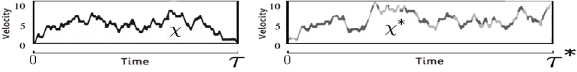
Figure 2: On the left: A Bessel excursion in velocity space, follows ${\dot{v}=-1/v+\sqrt{2D}\Gamma(t)}$, with the path constrained to start at ${v(0)=\epsilon}$ and end at ${v(\tau)=0}$, and remain strictly positive in the time interval ${(0,\tau)}$. The random area under the path is ${\chi}$. On the right: A velocity Bessel meander, with duration ${\tau^{*}}$ and area ${\chi^{*}}$, starts at ${v(0)=\epsilon}$ and remains positive, while the final value ${v(\tau^{*})}$ is random.

Nonormalizable limit function for the PDF. Using the long-time asymptotic moments provided in Eq. (6), in the moment-generating function, Eq. (2), yields an approximation for ${\hat{P}_{t}(k)}$, which we denote ${\hat{P}_{t}^{A}(k)}$, valid at long times:

$$\qquad\hat{P}_{t}^{A}(k)=1+t^{-3\nu/2+1}\sum_{n=1}^{\infty}\frac{(-1)^{n}{g^{*}}(kt^{3/2})^{2n}}{\langle\tau\rangle(2n)!}\times$$

$$\left[\int_{-\infty}^{\infty}\chi^{2n}B_{E}(\chi){\rm{d}}\chi\left(\frac{1}{{3n}-3\nu/2}-\frac{1}{3n-3\nu/2+1}\right)+\right.$$

$$\qquad\left.\int_{-\infty}^{\infty}\chi^{2n}B_{M}(\chi){\rm{d}}\chi\frac{2}{3\nu(3n-3\nu/2+1)}\right].$$ (8)

Rearranging, and using the Taylor expansion ${\cos\left(\omega^{3/2}y\right)=\sum_{n=0}^{\infty}(-1)^{n}\left(\omega^{3/2}y\right)^{2n}/(2n)!}$ for the summation, we obtain

$$\hat{P}_{t}^{A}(k) =1+\frac{{g^{*}}t^{-3\nu/2+1}}{\langle\tau\rangle}\int_{-\infty}^{\infty}{\rm{d}}\chi\int_{0}^{1}{\rm{d}}{}\omega\left[\cos\left(\omega^{3/2}k{\chi}t^{3/2}\right)-1\right]$$

$$\times\left[\frac{B_{E}({\chi})}{\omega^{3\nu/2-1}}+\frac{2B_{M}({\chi})-3\nu B_{E}({\chi})}{3\nu\omega^{3\nu/2}}\right].$$ (9)

Immediately below, taking the inverse-Fourier transform from ${k\rightarrow x}$, we drop the term proportional to ${\delta(x)}$, since this analysis applies only at large ${x}$. Calculating the integral over ${\omega}$, we now obtain the limit function ${\mathcal{I}(z)}$, explicitly, which describes the particle packet from its relation to the appropriately rescaled density via Eq. (5). In the limit ${z=x/t^{3/2}\ll 1}$:

$${\mathcal{I}({z})\approx\frac{{g^{*}}}{3\langle\tau\rangle}\langle{|\chi|^{\nu}\rangle}_{E}{|{z}|^{-\nu-1}},}$$ (10)

where ${\langle|\chi|^{\nu}\rangle}$ is the ${\nu}$’th absolute-moment of the excursion Kessler et al. [2014]. Note that this equation means that ${\mathcal{I}(z)}$ is nonintegrable around the origin. For ${z\gg 1}$:

$$\centering{\mathcal{I}({z})\approx\frac{4{g^{*}}}{9\nu\langle\tau\rangle}{{|z|}^{-\nu-1/3}}\int_{z}^{\infty}{|\chi|^{\nu-2/3}}B_{M}(\chi){\rm{d}}\chi.}\@add@centering$$ (11)

The function ${\mathcal{I}(z)}$ is called the infinite-covariant density (ICD), of the spatial diffusion of the cold atoms. The term infinite, means that it is nonnormalizable, despite being a limit function of the (obviously normalized) PDF. The term covariant refers to the fact that it is a function of the scaled variable ${x/t^{3/2}}$. We were able to obtain this nonnormalizable solution from the standard moment-generating function since in Eq. (2) we summed over the long-times asymptotic approximation, rather then the exact moments. Eq. (11) is the long-time asymptotics of the tail of the PDF, and in that sense it describes the rare fluctuations of the system. Fig. 1, confirms the convergence of Langevin simulation results, obtained by numerical integration of Eq. (1) at increasing times, to the nonnormalised density and its asymptotic approximations, Eqs. (10,11). These asymptotic limits are controlled exclusively by the excursions for $z\ll 1$ and the meander for $z\gg 1$, thus the far tail is described by a path that did not switch its velocity direction for a duration of the order of measurement time. Clearly, this is a rare event.

For every ${z}$:

$$\mathcal{I}(z)=\frac{2{g^{*}}}{3\langle\tau\rangle}\frac{1}{|{z}|^{\nu+1}}\left[\int_{|{z}|}^{\infty}B_{E}(\chi)|\chi|^{\nu}{\rm{d}}\chi+|z|^{2/3}\int_{|{z}|}^{\infty}\left(\frac{2}{3\nu}B_{M}(\chi)-B_{E}(\chi)\right){|\chi|^{\nu-2/3}}{\rm{d}}\chi\right].$$ (12)

Explicit expressions for the areal distributions, ${B_{E}(\chi)}$ and ${B_{M}(\chi)}$, used with Eq. (12) to plot the theory in Fig. 1, are provided in the SM. The ICD, ${\mathcal{I}(z)}$, gives the long times limit of all the absolute integer and fractional moments ${\langle|x|^{q}\rangle}$ of order ${q>\nu}$. Remarkably, this also includes the second moment, generally considered in many experiments as the typical characterization of a diffusion process. Looking back at Eq. (6): The mean squared-displacement, which is sensitive to the large fluctuations and the tails of the PDF, is obtained via ${\langle x^{2}(t)\rangle=t^{4-3\nu/2}\langle z^{2}\rangle_{\mathcal{I}}}$, where ${\langle z^{2}\rangle_{\mathcal{I}}=\int_{-\infty}^{\infty}z^{2}\mathcal{I}\left(z\right){\rm{d}}z}$. For every ${q\in\mathbb{R}}$: if ${\mathcal{I}(z)}$, Eq. (12), is integrable with respect to ${|z|^{q}}$, then the ICD determines ${\langle|x|^{q}(t)\rangle}$ (i.e., the ${q}$’th absolute-moment ) via ${\langle|x|^{q}(t)\rangle=t^{3q/2-3\nu/2+1}\langle|z|^{q}\rangle_{\mathcal{I}}}$, where ${\langle|z|^{q}\rangle_{\mathcal{I}}=\int_{-\infty}^{\infty}|z|^{q}\mathcal{I}\left(z\right){\rm{d}}z}$. Contrarily, when ${q\leq\nu}$, ${\mathcal{I}(z)}$ is nonintegrable with respect to the observable ${|z|^{q}}$, hence the moments which are less sensitive to large fluctuations are given by the Lévy distribution, as was found in Kessler and Barkai [2012]. This second long-time limit function has the scaling shape ${t^{-1/\nu}\mathcal{L}_{\nu}(x/t^{1/\nu})}$ Kessler and Barkai [2012]. For all the absolute-moments we find the bi-scaling behavior

$$\langle|x|^{q}(t)\rangle\propto\begin{cases}t^{q/\nu}\quad\quad\quad\quad\quad\quad q<\nu\\ t^{3q/2-3\nu/2+1}\quad\quad q>\nu\end{cases}.$$ (13)

Such multifractality is known as strong anomalous diffusion  Castiglione et al. [1999]. It represents the multi-scaling nature of the underlying PDF. Note that as ${q\rightarrow\nu}$ from above, the coefficient of ${\langle|x|^{q}\rangle}$, given by the analytic continuation of Eq. (6), diverges. The same happens when evaluating the moments using the Lévy scaling function, and approaching ${\nu}$ from below.

The derivation of ${\mathcal{I}(z)}$, Eq. (12), was performed in the limited range of ${D}$ where the variance is provided by the ICD. However, the scaling arguments at the beginning of this letter suggest that such a function should be found whenever the power-law equilibrium state in velocity space, Eq. (3), exists, namely for all ${0<D<1}$. Indeed, one can show that the ICD is valid also in the range ${0<D<1/5}$, where one finds that ${\langle x^{2}\rangle}$ grows linearly in time and the central part of the spreading packet is Gaussian. Even in this Gaussian regime, standard large-deviations theory does not apply and instead, the ICD given by Eqs. (5,12) insures the finiteness of large moments, beyond the mean squared-displacement. There is a delicate matching problem between the Gaussian packet and the pole of the ICD that describes the rare events, which we will address elsewhere.

Generality of the infinite-covariant density approach. We suggest that ICDs may be naturally related to multi-fractality (see physical examples below). In particular we now derive a rather general relation between exponents describing the bi-fractal moments, the central part of the packet (i.e., the bulk fluctuations, described by the Lévy CLT), and the exponents describing the ICD. When absolute-moments of order ${q>q_{c}}$, where ${q_{c}>0}$ defines some critical moment, scale faster in time than smaller ones, a scaling function ${\mathcal{I}(\tilde{z}=x/t^{\alpha})}$ describes the large fluctuations at long times via ${\langle|x|^{q}(t)\rangle\rightarrow t^{q\alpha-\beta+\alpha}\int_{-\infty}^{\infty}|\tilde{z}|^{q}\mathcal{I}(\tilde{z}){\rm{d}}\tilde{z}}$ (${\beta>\alpha>0}$). In this case one may find that ${\mathcal{I}(\tilde{z})=\lim_{t\rightarrow\infty}t^{\beta}P_{t}(x)}$, where ${P_{t}(x)}$ is the normalized PDF. This limit function is hence a nonnormalizable ICD (since obviously ${\langle x^{0}(t)\rangle=1}$, then ${\int_{-\infty}^{\infty}\mathcal{I}(\tilde{z}){\rm{d}}{\tilde{z}}\rightarrow\infty}$). In the case that around the origin the PDF is represented by a Lévy distribution of the form ${t^{-1/\gamma}\mathcal{L_{\gamma}}(x/t^{1/\gamma})}$ Klafter and Zumofen [1994], one will find (by “stitching” this limit function and the ICD at a central region of ${x}$, as in Rebenshtok et al. [2014a]) the following relation between the scaling exponents: ${\alpha-\beta+\alpha\gamma=1.}$ Indeed, in our case, ${(\alpha,\beta)=(3/2,1+1/(2D))}$ gives the correct ${\gamma=(1+D)/3D=\nu}$. In  Dentz et al. [2015], for example, the authors study a nonlinearly coupled continuous-time random walk with ${(\alpha,\beta)=(\bm{\alpha},\bm{\alpha}+\bm{\beta}-1)}$, which according to our analysis yields ${\gamma=\bm{\beta}/\bm{\alpha}}$ (${\bm{\alpha},\bm{\beta}}$ refer to the parameters in this Ref.). Our prediction is consistent with the result of their analysis. A more general relation links the exponents ${\alpha,\beta}$, of the ICD and the central power-law where ${x\sim t^{1/\gamma}}$, to the critical moment of the bi-scaling, ${q_{c}}$: ${\alpha-\beta+q_{c}\alpha=q_{c}/\gamma}$. This is consistent e.g., with the exponents found for transport on ${2}$-dimensional Lévy quasicrystals, studied in Buonsante et al. [2011]. The agreement with Dentz et al. [2015]; Buonsante et al. [2011] suggests an ICD in these systems too.

While non-analytical behavior of the moments raises a red flag for standard large-deviations theory, it promotes the use of the ICD approach. Finding this function is crucial for characterizing the rare events. The limit law given by the ICD in Eq. (5) for the rescaled PDF provides an alternative to the large-deviations principle, according to which the decay of the tails in thin-tailed systems may be controlled by some rate function ${Q(x/t)}$, such that ${Q(x/t)=\lim_{t\rightarrow\infty}\ln\left[P_{t}(x)\right]/t}$.

Discussion. CLTs play an important role in statistical physics, but of no less importance may be the proper characterization of the deviations from them. The ICD was previously found, for example, for different models of Lévy walks Rebenshtok et al. [2014a, b]. Since dual scaling of the moments and fat tailed distributions are very common, we speculate that ICDs will describe a large class of systems, e.g., Lévy glasses Bernabó et al. [2014], fluctuating surfaces Zamorategui et al. [2016], motion of tracer particles in the cell Gal and Weihs [2010] and diffusion on lipid bilayers Krapf et al. [2016]. To identify the ICDs in these diverse systems requires further work. Here, we have derived the ICD from the semiclassical description of cold atoms. This system is unique since it allows us, by tuning the intensity of the lasers, to find regimes where large deviations in the tails are non-negligible. In this case the rare events are important since they determine prominent statistical properties of the system, such as the mean squared-displacement. Our ICD is complementary to Lévy’s CLT in the sense that it solves the serious problem of the diverging variance expected by the Lévy distribution, although the latter insures the normalizability of the PDF. A full description of the system requires both functions.

Our work leaves open many interesting questions. One is the shape of the ICD when prior to measurement, the spreading particles are left to relax by interacting with the lasers in a spatial trap for some time ${t^{*}}$, where ${t^{*}\gg t}$. Our results apply in the opposite limit. In a previous work, Dechant and Lutz Dechant and Lutz [2012] find not bi-scaling, but tri-scaling of the moments in this case. In general, the ICD may depend on the protocol of the preparation of the system. In particular, the dependence on $t^{*}$ leads to aging effects, i.e., transport that depends on the preparation time. Finally, we point out that the function, ${f(z,\tilde{v})}$ (where ${\tilde{v}=v/t^{1/2}}$) in Eq. (4), is itself an ICD, as it is clearly not normalizable. Elucidating the properties of this ICD is an important future goal.

This work was supported by the Israel Science Foundation.

I Supplementary Material for:
Large deviations for spatial diffusion of cold atoms

I.1 A. Sisyphus cooling

Sisyphus cooling Cohen-Tannoudji and Phillips [1990] uses two coherent orthogonal, linearly-polarized laser beams, in a $1$-dimensional lin$\perp$lin configuration. The counter propagating lasers are projected onto a packet of hydrogen-like atoms (e.g., ⁸⁷Rb), creating an optical lattice. The cooling mechanism is driven by the coupled effect of periodic potential energy shifts, experienced by the particle as it moves along the lattice, and precisely timed, repeated, optical pumping events, which make the atom effectively move constantly “up” a potential hill (and hence the name Sisyphus cooling is appropriate). This induces a secular loss of kinetic energy for the atoms. In the semicalssical approximation one performs an average over the spatial modulation of the optical lattice, which works especially well in the limit of relatively fast particles.

In physical units, the deterministic damping force induced by the lasers may be written, as Cohen-Tannoudji and Phillips [1990]; Marksteiner et al. [1996]:

$${F(\tilde{p})=-\frac{{\bar{\alpha}\tilde{p}}}{1+(\tilde{p}/p_{c})^{2}},\qquad\mbox{where}\qquad\bar{\alpha}=\frac{12\pi^{2}\hbar|\delta|}{\lambda^{2}m\Gamma},\qquad\mbox{and}\qquad p_{c}=m\lambda/(4\pi\tau_{p}).}$$ (14)

Here, ${\tilde{p}}$ is the momentum of the atom, and $p_{c}$ is set by the velocity for which the atom travels the distance between two maximum points of the optical lattice in the time span of one optical pumping; ${\tau_{p}={9}/(2\Gamma s_{0})}$. The spatial periodicity of the optical lattice is half the wavelength, ${\lambda}$, of the lasers Cohen-Tannoudji and Phillips [1990]. The dimensionless saturation parameter; $s_{0}={2\Omega_{R}^{2}}/({4\delta^{2}+\Gamma^{2}})$, is dependent on the parameters of the laser and the lifetime of the excited state of the atom. The Rabi frequency is $\Omega_{R}$ and ${\delta=\omega_{l}-\omega_{R}}$ is the detuning between the laser frequency and the atom’s electronic transition frequency.

Since Sisyphus cooling is driven by quantum effects, instead of a monotonic decrease of the particle’s velocity, one finds momentum fluctuations, which in the semiclassical approximation are treated as a Gaussian white-noise in ${p}$ space Cohen-Tannoudji and Phillips [1990]. The time-development of the phase-space density, ${W_{\tilde{t}}({\tilde{x}},{\tilde{p}})}$, at time ${{\tilde{t}}}$ is given by Kramer’s Eq. Marksteiner et al. [1996],

$${\frac{\partial W_{\tilde{t}}({\tilde{x}},{\tilde{p}})}{\partial{\tilde{t}}}+{\tilde{p}}\frac{\partial W_{\tilde{t}}({\tilde{x}},{\tilde{p}})}{\partial{\tilde{x}}}=\left[\tilde{D}\frac{\partial^{2}}{\partial^{2}{\tilde{p}}}-\frac{\partial}{\partial{\tilde{p}}}F({\tilde{p}})\right]W_{\tilde{t}}({\tilde{x}},{\tilde{p}).}}$$ (15)

The amplitude of the momentum fluctuations has two components:

$${\tilde{D}=D_{1}+\frac{D_{2}}{1+({\tilde{p}}/p_{c})^{2}},\qquad\mbox{where}\qquad D_{1}=11mE_{R}/(2\tau_{p})\qquad\mbox{and}\qquad{D_{2}=9\pi^{2}U_{0}^{2}/(\lambda^{2}s_{0}\Gamma)}.}$$ (16)

Here, ${E_{R}=2\pi^{2}h^{2}/(m\lambda^{2})}$ is the recoil energy, and ${U_{0}=\frac{2}{3}\hbar\delta s_{0}}$ is the depth of the optical lattice Cohen-Tannoudji and Phillips [1990]. The first component of the fluctuations, $D_{1}$, is the result of the recoil due to the emission of the photon during the optical pumping. The second component relates to emissions occurring in “the wrong points” on the optical lattice, which result in temporary gains of kinetic energy (when the atom “slides” down the potential). For slow particles, ${\tilde{D}\sim D_{1}+D_{2}}$, while for fast particles, ${\tilde{D}\sim D_{1}}$. From Eq. (14), the cooling-force is small when acting on fast particles, hence these particles tend to remain fast for long times and in the range of D in which we are interested in the main text, they dominate the statistical properties of the diffusing packet. We therefore neglect the contribution of $D_{2}$, and use $\tilde{D}=D_{1}$ (this agrees with simulations, see e.g. Dechant et al. [2016]).

Finally, we work in dimensionless units, ${(x,p,t)}$, where Barkai et al. [2014]; Dechant et al. [2016]:

$${p=\tilde{p}/p_{c},\qquad{t=\tilde{t}\bar{\alpha}}\qquad\textrm{and}\qquad{x=\tilde{x}\bar{\alpha}m/p_{c}}.}$$ (17)

Note that we take the particle’s mass to be $m=1$ for convenience, hence in the main text ${p=v}$, where ${v}$ is the dimensionless velocity (and we can set ${p_{c}=v_{c}=1}$). In these units, ${D=\tilde{D}/\left[p_{c}^{2}\bar{\alpha}\right]=cE_{R}/U_{0}}$, where ${c\approx 22}$, and the dimensionless Langevin Eq. (${1}$), in the main text, is the equivalent of the Kramers equation (15) above. Note that the constant ${c}$ may differ between different theoretical works and experiments, since the exact numbers in Eq. (16) depend on the details of the estimation of the noise in different experimental setups, and the particular atomic transition. In the main text we consider the range $0<D<1$, which translates to ${0<D_{1}/[p_{c}^{2}\bar{\alpha}]<1.}$

I.2 B. Excursions approach for solving the Langevin equation

Here we present the derivation of the relation between the probability density functions (PDFs) of the area under the Bessel excursion and Bessel meander, and the Sisyphus-cooled particles’ position PDF, ${P_{t}(x)}$, at time ${t}$ Barkai et al. [2014]. We call this relation the modified Montroll-Weiss equation (see Montroll and Weiss [1965]). We repeat this derivation here, which we first presented in Barkai et al. [2014], since it is a bit different then the famous original relation (see [SM1] for a review), due to the specific treatment given to the meander (which is separate from the excursions). This modified equation is the starting point for our calculation of the integer moments ${\langle|x|^{2m}\rangle}$ for ${m\geq 1}$, Eq. (${6}$) in the main text. As mentioned there, we use the zero crossings of the Markovian process, ${v(t)}$ (Eq. (${1}$) in the main text), to define the waiting times ${\left\{\tau_{i}\right\}}$ and the corresponding excursions with areas ${\left\{\chi_{i}\right\}}$. The joint distributions for the area and the duration of an excursion is

$$\Phi_{E}\left(\chi,\tau\right)\sim g(\tau)\phi_{E}(\chi|\tau).$$ (18)

Here ${g(\tau}$) is the first-passage time PDF of the process ${v(t)}$, from ${\epsilon}$ to zero (eventually ${\epsilon}$ is taken to zero and cancels out, see Barkai et al. [2014]), and $\phi_{E}(\chi|\tau)$ is the conditional PDF for ${\chi}$ given ${\tau}$. This density has the scaling form Barkai et al. [2014]

$$\phi_{E}\left(\chi|\tau\right)\sim\frac{1}{\tau^{3/2}}B_{E}\left(\frac{\chi}{\tau^{3/2}}\right).$$ (19)

Let $\eta_{s}(x,t){\rm d}t{\rm d}x$ be the probability that the particle crossed the zero velocity state, $v=0$, for the $s$th time in the time interval $(t,t+{\rm d}t)$, and that its position is in the interval $(x,x+{\rm d}x)$. This probability is related to the the previous crossing via

$$\eta_{s}(x,t)=\int_{-\infty}^{\infty}{\rm d}{\chi}\int_{0}^{t}{\rm d}\tau\,\eta_{s-1}\left(x-{\chi},t-\tau\right){1\over\tau^{{3/2}}}B_{E}\left({\chi\over\tau^{{3/2}}}\right)g\left(\tau\right),$$ (20)

where we have used Eqs. (18,19). Changing variables from ${\chi}\rightarrow\zeta\tau^{{3/2}}$ we obtain

$$\eta_{s}(x,t)=\int_{-\infty}^{\infty}\!\!{\rm d}\zeta\int_{0}^{\infty}\!\!{\rm d}\tau\,\eta_{s-1}\left(x-\zeta\tau^{3/2},t-\tau\right)B_{E}\left(\zeta\right)g\left(\tau\right).$$ (21)

The process is now described by a sequence of waiting times $\tau_{1},\tau_{2},...$ and the corresponding scaled displacements $\zeta_{1},\zeta_{2},...$. The displacement in the $s$th interval is

$${\chi}_{s}=\zeta_{s}\tau_{s}^{3/2}$$ (22)

The advantage of this representation of the problem, in terms of the pair of microscopic stochastic variables $\tau,\zeta$ (instead of the correlated pair $\tau,\chi$), is that we may treat $\zeta$ and $\tau$ as independent random variables whose corresponding PDFs are $g(\tau)$ and $B_{E}(\zeta)$ respectively. Here $\tau>0$ and $-\infty<\zeta<\infty$. The initial condition $x=0$ at time $t=0$ implies $\eta_{0}(x,t)=\delta(x)\delta(t)$. The probability, $P_{t}(x)$, of finding the particle in $(x,x+{\rm d}x)$ at time $t$, is obtained from the relation

$$P_{t}(x)=\sum_{s=0}^{\infty}\int_{-\infty}^{\infty}{\rm d}\zeta\int_{0}^{t}{\rm d}\tau^{*}\,\eta_{s}\left(x-\zeta{\tau^{*}}^{3/2},t-\tau^{*}\right)B_{M}\left(\zeta\right)w\left(\tau^{*}\right).$$ (23)

Here we used Eq. (19), and since the last jump event took place at $t-\tau^{*}$, and in the time period $(t-\tau^{*},t)$ the particle did not cross the velocity origin, as mentioned, the last time interval in the sequence is described by a meander. By definition; $w(\tau^{*})=1-\int_{0}^{\tau}g(\tau^{*}){\rm d}\tau^{*}$ is the survival probability. The probability to have a meander with an area ${\chi^{*}}$ underneath it, and duration $\tau^{*}$, is

$${\Psi_{M}\left(\chi^{*},\tau^{*}\right)=\frac{1}{{\tau^{*}}^{3/2}}w(\tau^{*})B_{M}(\frac{\chi^{*}}{{\tau^{*}}^{3/2}}).}$$ (24)

We provide explicit expressions for ${B_{E}(\zeta)}$ and ${B_{M}(\zeta)}$ below. The summation in Eq. (23) is performed over all the possible realizations with $s$ returns to the velocity origin, $v=0$. In Laplace $t\to u$ and Fourier $x\to k$ spaces, using the convolution theorem and Eq. (21), we find

$$\hat{\eta}_{s}\left(k,u\right)=\hat{\eta}_{s-1}\left(k,u\right)LT\left[\hat{B}_{E}\left(k\tau^{3/2}\right)g\left(\tau\right)\right],$$ (25)

where $LT[\cdot]$ means Laplace transform, and

$$\hat{B}_{E}\left(k\tau^{3/2}\right)=\int_{-\infty}^{\infty}\exp\left(ik\zeta{\tau^{3/2}}\right)B_{E}(\zeta){\rm d}\zeta.$$ (26)

Hence ${\hat{\eta}_{s}(k,u)=\hat{\Phi}_{E}(k,u)\hat{\eta}_{s-1}(k,u).}$ This implies that

$$\hat{\eta}_{s}(k,u)=\left[\hat{\Phi}_{E}(k,u)\right]^{s},$$ (27)

reflecting the renewal property of the underlying random walk. Summing the Fourier and Laplace transform of Eq. (23), applying the convolution theorem and using Eq. (27), we find the modified Montroll-Weiss equation for the Fourier and Laplace transform of $P(x,t)$:

$${\hat{P}_{u}(k)={\hat{\Psi}_{M}(k,u)\over 1-\hat{\Phi}_{E}\left({k,u}\right)}.}$$ (28)

I.3 C. Area distribution under the Bessel excursion and Bessel meander

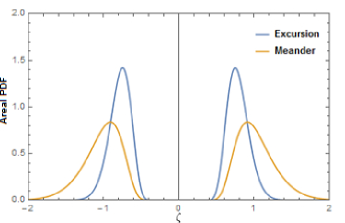
Figure 3: (Color online) The areal distributions, ${B_{E}(\chi)}$ and ${B_{M}(\chi)}$, of the area under the (positive and negative) Bessel excursion and Bessel meander with ${D=0.4}$, are presented in (blue) and (orange), respectively.

The symmetric area distribution ${B_{E}(\zeta)}$, for the scaled area ${\zeta=\chi/\tau^{3/2}}$ under the Bessel excursion of duration ${\tau}$ (which takes into account both the paths that always remain positive, and those which remain negative) is Barkai et al. [2014]; Kessler et al. [2014]

$$B_{E}(\zeta) = -\frac{\Gamma(1+\alpha)}{4\pi|\zeta|}\left(\frac{4D^{1/3}}{|\zeta|^{2/3}}\right)^{\frac{3\nu}{2}+1}\sum_{k}[{d}_{k}]^{2}\left[\Gamma\left(\frac{5}{3}+\nu\right)\sin\left(\pi\frac{2+3\nu}{3}\right){}_{2}F_{2}\left(\frac{4}{3}+\frac{\nu}{2},\frac{5}{6}+\frac{\nu}{2};\frac{1}{3},\frac{2}{3};-\frac{4D\lambda_{k}^{3}}{27\zeta^{2}}\right)\right.$$ (29)

$$\qquad\qquad\qquad{}-\frac{D^{1/3}\lambda_{k}}{|\zeta|^{2/3}}\Gamma\left(\frac{7}{3}+\nu\right)\sin\left(\pi\frac{4+3\nu}{3}\right){}_{2}F_{2}\left(\frac{7}{6}+\frac{\nu}{2},\frac{5}{3}+\frac{\nu}{2};\frac{2}{3},\frac{4}{3};-\frac{4D\lambda_{k}^{3}}{27\zeta^{2}}\right)$$

$$\qquad\qquad\qquad\left.{}+\frac{1}{2}\left(\frac{D^{1/3}\lambda_{k}}{|\zeta|^{2/3}}\right)^{2}\Gamma\left(3+\nu\right)\sin\left(\pi\nu\right){}_{2}F_{2}\left(2+\frac{\nu}{2},\frac{3}{2}+\frac{\nu}{2};\frac{4}{3},\frac{5}{3};-\frac{4D\lambda_{k}^{3}}{27\zeta^{2}}\right)\right].$$

Here ${{}_{2}F_{2}(\cdot)}$ is a hypergeometric function [SM2]. Eq. (29) is called the Bessel distribution, and it is plotted in Fig. 3. The method used for finding these areal distributions in Barkai et al. [2014]; Kessler et al. [2014], employed an eigenfunction expansion of the solution to the Feynman-Kac formula Barkai et al. [2014]. This formula is used for finding the distributions of functionals of a stochastic path, in our case this is ${\chi_{i}=\int_{t_{i-1}}^{t_{i-1}+\tau_{i}}{v(t^{\prime}){\rm{d}}t^{\prime}}}$ and ${v(t^{\prime})}$ is the velocity trajectory corresponding to the Langevin Eq. ${\dot{v}=-1/v+\sqrt{2D}\Gamma(t)}$. Note that we use the large ${v}$ behavior of ${F(v)=-v/(1+v^{2})}$ (the Sisyphus cooling force in dimensionless units, as explained), physically this works well since we are interested in the far tails of the spatial density of the particle packet, where small scale velocities are unimportant. The summation in Eqs. (29,30) is performed over ${k}$ modes, where ${\lambda_{k}}$ are the eigenvalues of the time independent Schröedinger-like equation Barkai et al. [2014], ${d_{k}}$ is the normalization of the ${k}$th eigenfunction Barkai et al. [2014]. These parameters are found numerically; the method is explained in detail in Barkai et al. [2014]. Asymptotic analytic approximations and further discussion about the meaning of these parameters appear in Kessler et al. [2014]. Similarly, the distribution of the area under a Bessel meander is

$$B_{M}(\zeta) =-\frac{\Gamma\left(1+\alpha\right)}{2\pi|\zeta|}\left(\frac{4^{3/2}D^{1/2}}{|\zeta|}\right)^{\nu}\sum_{k}{d_{k}}a_{k}\left[\Gamma\left(1+\nu\right)\sin\left(\pi\nu\right){}_{2}F_{2}\left(\frac{\nu}{2}+1,\frac{\nu}{2}+\frac{1}{2};\frac{1}{3},\frac{2}{3};\frac{-4D\lambda_{k}^{3}}{27\zeta^{2}}\right)\right.$$ (30)

$$-\left(\frac{D^{1/3}\lambda_{k}}{|\zeta|^{2/3}}\right)\Gamma\left(\frac{5}{3}+\nu\right)\sin\left(\pi\frac{2+3\nu}{3}\right){}_{2}F_{2}\left(\frac{\nu}{2}+\frac{4}{3},\frac{\nu}{2}+\frac{5}{6};\frac{2}{3},\frac{4}{3};\frac{-4D\lambda_{k}^{3}}{27\zeta^{2}}\right)$$

$$\left.+\frac{1}{2}\left(\frac{D{1/3}\lambda_{k}}{|\zeta|^{2/3}}\right)^{2}\Gamma\left(\frac{7}{3}+\nu\right)\sin\left(\pi\frac{4+3\nu}{3}\right){}_{2}F_{2}\left(\frac{\nu}{2}+\frac{7}{6},\frac{\nu}{2}+\frac{5}{3};\frac{4}{3},\frac{5}{3};\frac{-4D\lambda_{k}^{3}}{27\zeta^{2}}\right)\right].$$

This distribution is also plotted in Fig. 3. The numerical parameter, ${a_{k}}$ is evaluated by integration of the eigenfunction over ${v^{1/(2D)}}$ Barkai et al. [2014]. In Table 1, we provide ${10}$ values, for example, for ${\lambda_{k},d_{k}}$ and ${a_{k}}$, with ${D=0.4}$ and ${D=0.5}$, which are sufficient for a good approximation of the distributions.

${D}$	${k\rightarrow}$	$1$	$2$	$3$	$4$	$5$	$6$	$7$	$8$	$9$	$10$
$0.4$	$\lambda_{k}$	$3.593$	$5.075$	$6.3855$	$7.5581$	$8.657$	$9.691$	$10.673$	$11.613$	$12.515$	$13.387$
	$d_{k}$	$0.4159$	$0.57$	$0.682$	$0.773$	$0.851$	$0.920$	$0.983$	$1.042$	$1.095$	$1.145$
	$a_{k}$	$0.849$	$0.314$	$0.535$	$0.307$	$0.441$	$0.295$	$0.3915$	$0.284$	$0.359$	$0.274$
$0.5$	$\lambda_{k}$	$3.37$	$4.89$	$6.21$	$7.41$	$8.52$	$9.56$	$10.55$	$11.5$	$12.4$	$13.28$
	$d_{k}$	$0.521$	$0.675$	$0.78$	$0.879$	$0.94$	$0.997$	$1.076$	$1.102$	$1.151$	$1.221$
	$a_{k}$	$1.040$	$0.239$	$0.604$	$0.244$	$0.475$	$0.225$	$0.414$	$0.215$	$0.365$	$0.217$

Table 1: The first $10$ numeric coefficients, $\lambda_{k}$, $d_{k}$ and $a_{k}$, required for plotting the theoretical PDFs, Eqs. (29,30), with ${D=0.4}$ and ${0.5}$. These coefficients were calculated using the method explained in Barkai et al. [2014]. As explained, these values are also required for plotting the ICD, ${\mathcal{I}(z)}$, Eq. (${12}$) in the main text. For this purpose as well, we found that ${10}$ ${k}$-modes are sufficient.

I.4 D. Derivation of the moments

We derive the moments ${\langle x^{2m}\rangle}$, for ${m=1,2,...}$, presented in Eq. (${7}$) in the main text. Our starting point is Eq. (28) and the areal distribution of the excursions. Applying Fourier ${x\rightarrow k}$ and Laplace ${t\rightarrow u}$ transforms to Eq. (18), using Eq. (19), we write

$${\hat{\Phi}_{E}\left(k,u\right)=\int_{-\infty}^{\infty}{d\chi\int_{0}^{\infty}{d\tau e^{-u\tau+ik\chi}g\left(\tau\right)\frac{1}{\tau^{3/2}}B_{E}\left(\frac{\chi}{\tau^{3/2}}\right)}}.}$$ (31)

Note that the distribution ${g(\tau)}$ is given by the solution of a standard first passage time problem in Marksteiner et al. [1996]. Asymptotically,

$$g(\tau)\approx g_{*}\tau^{-1-3\nu/2},\quad\mbox{for}\quad\tau\gg 1$$ (32)

where ${\nu=1/(3D)+1/3}$ and (see Barkai et al. [2014])

$$\frac{g_{*}}{\langle\tau\rangle}=\frac{2D}{\sqrt{\pi}}\frac{(1+D)\Gamma(\frac{1}{2D})}{(4D)^{\frac{1+D}{2D}}\Gamma(\frac{1-D}{2D})\Gamma(\frac{1+D}{2D})}.$$ (33)

Expanding the exponent ${e^{ik\chi}}$ in Eq. (31) as a Taylor series for small ${k}$, using Eq. (33), while separating out the ${n=0}$’th term, we obtain

$$\hat{\Phi}_{E}(k,u)=\hat{g}(u)+\sum_{m=1}^{\infty}{\frac{(ik)^{m}}{m!}\langle\zeta^{m}\rangle_{E}{g^{*}}\Gamma(\frac{3m}{2}-\frac{3\nu}{2})u^{-\frac{3m}{2}+\frac{3\nu}{2}}},$$ (34)

where ${\hat{g}(u)=\int_{0}^{\infty}g(\tau)\exp(-u\tau){\rm{d}}\tau}$ and

$${\langle\zeta^{m}\rangle_{E}=\int_{-\infty}^{\infty}{\zeta^{m}B_{E}(\zeta){\rm{d}}{\zeta}}.}$$ (35)

Here, we changed variables to ${\zeta=\chi/\tau^{3/2}}$. Notice that ${B(\zeta)}$ is symmetric, hence its odd moments are zero. Using the equivalent procedure for $\hat{\psi}_{M}\left(k,u\right)$ with $B_{M}(\zeta)$, and using

$${\hat{w}(u)=\int_{0}^{\infty}{w(\tau)\exp(-u\tau){\rm{d}}\tau}=[1-\hat{g}(u)]/u,}$$ (36)

for the survival probability ${w(\tau)}$ (defined in Sec. B.), we rewrite Eq. (28) as

$$\hat{P}_{u}\left(k\right)=\frac{1}{u}\frac{1+\sum_{m=1}^{\infty}{\frac{(-1)^{m}}{\hat{w}(u)}\frac{2{g^{*}}}{3\nu}\Gamma({3m}-3\nu/2+1)\frac{1}{(2m)!}\langle\zeta^{2m}\rangle_{M}k^{2m}u^{-{3m}+3\nu/2-1}}}{1-\sum_{m=1}^{\infty}{\frac{(-1)^{m}}{1-\hat{g}(u)}{g^{*}}\Gamma({3m}-3\nu/2)\frac{1}{(2m)!}\langle\zeta^{2m}\rangle_{E}k^{2m}u^{-{3m}+3\nu/2}}}.$$ (37)

For ${2/3<\nu<2}$ (recall, we derive our main results in the range ${0<D<1}$), the average $\langle\tau\rangle$ is finite, therefore from Eqs. (28,32), the Laplace-transforms of ${g(\tau)}$ and ${w(\tau)}$, in the ${u\rightarrow 0}$ limit are

$$\hat{g}(u)\approx 1-u\langle\tau\rangle,\qquad\qquad\hat{w}(u)\approx\langle\tau\rangle.$$ (38)

By using the relation ${\langle x^{2m}\rangle=(-1)^{m}\left[{\rm{d}}^{2m}/{\rm{d}}k^{2m}\hat{P}_{u}(k)\right]|_{k=0}}$, we derive the moments in Eq. (${6}$), in the main text, in the long time limit.

(SM1) R. Metzler and J. Klafter, Physics reports 339, 1 (2000)
(SM2) M. Abramowitz and I. A Stegun, Handbook of Mathematical functions: with formulas, graphs, and mathematical tables (Courier Dover Publications, 1972).

References

- Gardiner [2009] C. Gardiner, Stochastic methods (Springer Berlin, 2009).
- Touchette [2009] H. Touchette, Physics Reports 478, 1 (2009).
- Ellis [1999] R. S. Ellis, Physica D: Nonlinear Phenomena 133, 106 (1999).
- Krapivsky et al. [2014] P. Krapivsky, K. Mallick, and T. Sadhu, Physical review letters 113, 078101 (2014).
- Meerson et al. [2016] B. Meerson, E. Katzav, and A. Vilenkin, Physical review letters 116, 070601 (2016).
- Hegde et al. [2014] C. Hegde, S. Sabhapandit, and A. Dhar, Physical review letters 113, 120601 (2014).
- Bouchaud and Georges [1990] J. P. Bouchaud and A. Georges, Physics Reports 195, 127 (1990).
- Klafter et al. [1996] J. Klafter, M. F. Shlesinger, and G. Zumofen, Physics today 49, 33 (1996).
- Zaburdaev et al. [2015] V. Zaburdaev, S. Denisov, and J. Klafter, Rev. Mod. Phys. 87, 483 (2015).
- Cohen-Tannoudji and Phillips [1990] C. Cohen-Tannoudji and W. D. Phillips, Phys. Today 43, 33 (1990).
- Marksteiner et al. [1996] S. Marksteiner, K. Ellinger, and P. Zoller, Physical Review A 53, 3409 (1996).
- Kessler and Barkai [2012] D. A. Kessler and E. Barkai, Physical Review Letters 108, 230602 (2012).
- Sagi et al. [2012] Y. Sagi, M. Brook, I. Almog, and N. Davidson, Physical Review Letters 108, 093002 (2012).
- Klafter and Sokolov [2011] J. Klafter and I. M. Sokolov, First steps in random walks: from tools to applications (Oxford University Press, 2011).
- Rebenshtok et al. [2014a] A. Rebenshtok, S. Denisov, P. Hänggi, and E. Barkai, Physical Review Letters 112, 110601 (2014a).
- Dalibard and Cohen-Tannoudji [1989] J. Dalibard and C. Cohen-Tannoudji, JOSA B 6, 2023 (1989).
- Kessler and Barkai [2010] D. A. Kessler and E. Barkai, Physical Review Letters 105, 120602 (2010).
- Douglas et al. [2006] P. Douglas, S. Bergamini, and F. Renzoni, Physical review letters 96, 110601 (2006).
- Katori et al. [1997] H. Katori, S. Schlipf, and H. Walther, Physical Review Letters 79, 2221 (1997).
- Note [1] Simulations were performed using standard Euler-Mayurama integration Gardiner [2009] of Eq. (1\@@italiccorr) with a step size of , for particles.
- Lutz [2004] E. Lutz, Physical review letters 93, 190602 (2004).
- Holz et al. [2015] P. C. Holz, A. Dechant, and E. Lutz, EPL (Europhysics Letters) 109, 23001 (2015).
- Dechant et al. [2016] A. Dechant, S. T. Shafier, D. A. Kessler, and E. Barkai, Physical Review E 94, 022151 (2016).
- Barkai et al. [2014] E. Barkai, E. Aghion, and D. A. Kessler, Physical Review X 4, 021036 (2014).
- Kessler et al. [2014] D. A. Kessler, S. Medalion, and E. Barkai, Journal of Statistical Physics 156, 686 (2014).
- Louchard [1984] G. Louchard, Journal of Applied Probability , 479 (1984).
- Pitman [1999] J. Pitman, Electron. J. Probab 4, 1 (1999).
- Majumdar and Orland [2015] S. N. Majumdar and H. Orland, Journal of Statistical Mechanics: Theory and Experiment 2015, P06039 (2015).
- Durrett et al. [1977] R. T. Durrett, D. L. Iglehart, and D. R. Miller, The Annals of Probability , 117 (1977).
- Schehr and Le Doussal [2010] G. Schehr and P. Le Doussal, Journal of Statistical Mechanics: Theory and Experiment 2010, P01009 (2010).
- Martin et al. [2011] E. Martin, U. Behn, and G. Germano, Physical Review E 83, 051115 (2011).
- Font-Clos and Moloney [2016] F. Font-Clos and N. R. Moloney, Physical Review E 94, 030102 (2016).
- Montroll and Weiss [1965] E. W. Montroll and G. H. Weiss, Journal of Mathematical Physics 6, 167 (1965).
- Note [2] Eq. (6\@@italiccorr) is analytically continued to absolute odd and fractional moments , for , by replacing and using and .
- Castiglione et al. [1999] P. Castiglione, A. Mazzino, P. Muratore-Ginanneschi, and A. Vulpiani, Physica D: Nonlinear Phenomena 134, 75 (1999).
- Klafter and Zumofen [1994] J. Klafter and G. Zumofen, Physical Review E 49, 4873 (1994).
- Dentz et al. [2015] M. Dentz, T. Le Borgne, D. R. Lester, and F. P. de Barros, Physical Review E 92, 032128 (2015).
- Buonsante et al. [2011] P. Buonsante, R. Burioni, and A. Vezzani, Physical Review E 84, 021105 (2011).
- Rebenshtok et al. [2014b] A. Rebenshtok, S. Denisov, P. Hänggi, and E. Barkai, Phys. Rev. E 90, 062135 (2014b).
- Bernabó et al. [2014] P. Bernabó, R. Burioni, S. Lepri, and A. Vezzani, Chaos, Solitons & Fractals 67, 11 (2014).
- Zamorategui et al. [2016] A. L. Zamorategui, V. Lecomte, and A. B. Kolton, Physical Review E 93, 042118 (2016).
- Gal and Weihs [2010] N. Gal and D. Weihs, Physical Review E 81, 020903 (2010).
- Krapf et al. [2016] D. Krapf, G. Campagnola, K. Nepal, and O. B. Peersen, Physical Chemistry Chemical Physics 18, 12633 (2016).
- Dechant and Lutz [2012] A. Dechant and E. Lutz, Physical Review Letters 108, 230601 (2012).