A Data-Oriented Model of Literary Language

Abstract

We consider the task of predicting how literary a text is, with a gold standard from human ratings. Aside from a standard bigram baseline, we apply rich syntactic tree fragments, mined from the training set, and a series of hand-picked features. Our model is the first to distinguish degrees of highly and less literary novels using a variety of lexical and syntactic features, and explains 76.0 % of the variation in literary ratings.

1 Introduction

What makes a literary novel literary? This seems first of all to be a value judgment; but to what extent is this judgment arbitrary, determined by social factors, or predictable as a function of the text? The last explanation is associated with the concept of literariness, the hypothesized linguistic and formal properties that distinguish literary language from other language [Baldick (2008]. Although the definition and demarcation of literature is fundamental to the field of literary studies, it has received surprisingly little empirical study. Common wisdom has it that literary distinction is attributed in social communication about novels and that it lies mostly outside of the text itself [Bourdieu (1996], but an increasing number of studies argue that in addition to social and historical explanations, textual features of various complexity may also contribute to the perception of literature by readers (cf. Harris, 1995; McDonald, 2007). The current paper shows that not only lexical features but also hierarchical syntactic features and other textual characteristics contribute to explaining judgments of literature.

Our main goal in this project is to answer the following question: are there particular textual conventions in literary novels that contribute to readers judging them to be literary? We address this question by building a model of literary evaluation to estimate the contribution of textual factors. This task has been considered before with a smaller set of novels (restricted to thrillers and literary novels), using bigrams [van Cranenburgh and Koolen (2015]. We extend this work by testing on a larger, more diverse corpus, and by applying rich syntactic features and several hand-picked features to the task. This task is first of all relevant to literary studies—to reveal to what extent literature is empirically associated with textual characteristics. However, practical applications are also possible; e.g., an automated model could help a literary publisher decide whether the work of a new author fits its audience; or it could be used as part of a recommender system for readers.

Literary language is arguably a subjective notion. A gold standard could be based on the expert opinions of critics and literary prizes, but we can also consider the reader directly, which, in the form of a crowdsourced survey, more easily provides a statistically adequate number of responses. We therefore base our gold standard on a large online survey of readers with ratings of novels.

Literature comprises some of the most rich and sophisticated language, yet stylometry typically does not exploit linguistic information beyond part-of-speech (pos) tags or grammar productions, when syntax is involved at all (cf. e.g., Stamatatos et al., 2009; Ashok et al., 2013). While our results confirm that simple features are highly effective, we also employ full syntactic analyses and argue for their usefulness. We consider tree fragments: arbitrarily-sized connected subgraphs of parse trees [Swanson and Charniak (2012, Bergsma et al. (2012, van Cranenburgh (2012]. Such features are central to the Data-Oriented Parsing framework [Scha (1990, Bod (1992], which postulates that language use derives from arbitrary chunks (e.g., syntactic tree fragments) of previous language experience. In our case, this suggests the following hypothesis.

Hypothesis 1: Literary authors employ a distinctive inventory of lexico-syntactic constructions (e.g., a register) that marks literary language.

Next we provide an analysis of these constructions which supports our second hypothesis.

Hypothesis 2: Literary language invokes a larger set of syntactic constructions when compared to the language of non-literary novels, and therefore more variety is observed in the parse tree fragments whose occurrence frequencies are correlated with literary ratings.

The support provided for these hypotheses suggests that the notion of literature can be explained, to a substantial extent, from textual factors, which contradicts the belief that external, social factors are more dominant than internal, textual factors.

Figure 1: A parse tree fragment from Franzen, The Corrections. Original sentence: something terrible was going to happen.

2 Task, experimental setup

We consider a regression problem of a set of novels and their literary ratings. These ratings have been obtained in a large reader survey (about 14k participants), in which 401 recent, bestselling Dutch novels (as well as works translated into Dutch) where rated on a 7-point Likert scale from definitely not to highly literary. The participants were presented with the author and title of each novel, and provided ratings for novels they had read. The ratings may have been influenced by well known authors or titles, but this does not affect the results of this paper because the machine learning models are not given such information. The task we consider is to predict the mean rating for each novel. We exclude 16 novels that have been rated by less than 50 participants. 91 % of the remaining novels have a $t$-distributed 95 % confidence interval $<0.5$; e.g., given a mean of 3, the confidence interval typically ranges from 2.75 to 3.25. Therefore for our purposes the ratings form a reliable consensus. Novels rated as highly literary have smaller confidence intervals, i.e., show a stronger consensus. Where a binary distinction is needed, we call a rating of 5 or higher ‘literary.’

Since we aim to extract relevant features from the texts themselves and the number of novels is relatively small, we apply cross-validation, so as to exploit the data to the fullest extent while maintaining an out-of-sample approach. We divide the corpus in 5 folds of roughly equal size, with the following constraints: (a) novels by the same author must be in the same fold, since we want to rule out any influence of author style on feature selection or model validation; (b) the distribution of literary ratings in each fold should be similar to the overall distribution (stratification).

We control for length and potential particularities of the start of novels by considering sentences 1000–2000 of each novel. 18 novels with fewer than 2000 sentences are excluded. Together with the constraint of at least 50 ratings, this brings the total number of novels we consider to 369.

We evaluate the effectiveness of the features using a ridge regression model, with 5-fold cross-validation; we do not tune the regularization. The results are presented incrementally, to illustrate the contribution of each feature relative to the features before it. This makes it possible to gauge the effective contribution of each feature while taking any overlap into account.

We use $R^{2}$ as the evaluation metric, expressing the percentage of variance explained (perfect score 100); this shows the improvement of the predictions over a baseline model that always predicts the mean value (4.2, in this dataset). A mean baseline model is therefore defined to have an $R^{2}$ of 0. Other baseline models, e.g., always predicting 3.5 or 7, attain negative $R^{2}$ scores, since they perform worse than the mean baseline. Similarly, a random baseline will yield a negative expected $R^{2}$.

3 Basic features

Sentence length, direct speech, vocabulary richness, and compressibility are simple yet effective stylometric features. We count direct speech sentences by matching on specific punctuation; this provides a measure of the amount of dialogue versus narrative text in the novel. Vocabulary richness is defined as the proportion of words in a text that appear in the top 3000 most common words of a large reference corpus (Sonar 500; Oostdijk et al., 2013); this shows the proportion of difficult or unusual words. Compressibility is defined as the bzip2 compression ratio of the texts; the intuition is that a repetitive and predictable text will be highly compressible. cliches is the number of cliché expressions in the texts based on an external dataset of 6641 clichés [van Wingerden and Hendriks (2015]; clichés, being marked as informal and unoriginal, are expected to be more prevalent in non-literary texts. Table 1 shows the results of these features. Several other features were also evaluated but were either not effective or did not achieve appreciable improvements when these basic features are taken into account; notably Flesch readability [Flesch (1948], average dependency length [Gibson (2000], and D-level [Covington et al. (2006].

	$R^{2}$
mean sent. len.	16.4
+ % direct speech sentences	23.1
+ top 3000 vocab.	23.5
+ bzip2_ratio	24.4
+ cliches	30.0

Table 1: Basic features, incremental scores.

4 Automatically induced features

In this section we consider extracting syntactic features, as well as three (sub)lexical baselines.

topics is a set of 50 topic weights induced with Latent Dirichlet Allocation (LDA; Blei et al., 2003) from the corpus (for details, cf. Jautze et al., 2016).

Furthermore, we use character and word $n$-gram features. For words, bigrams present a good trade off in terms of informativeness (a bigram frequency is more specific than the frequency of an individual word) and sparsity (three or more consecutive words results in a large number of $n$-gram types with low frequencies). For character $n$-grams, $n=4$ achieved good performance in previous work (e.g., Stamatatos, 2006).

We note three limitations of $n$-grams. First, the fixed $n$: larger or discontiguous chunks are not extracted. Combining $n$-grams does not help since a linear model cannot capture feature interactions, nor is the consecutive occurrence of two features captured in the bag-of-words representation. Second, larger $n$ imply a combinatorial explosion of possible features, which makes it desirable to select the most relevant features. Finally, word and character $n$-grams are surface features without linguistic abstraction. One way to overcome these limitations is to turn to syntactic parse trees and mine them for relevant features unrestricted in size.

Specifically, we consider tree fragments as features, which are arbitrarily-sized fragments of parse trees. If a parse tree is seen as consisting of a sequence of grammar productions, a tree fragment is a connected subsequence thereof. Compared to bag-of-word representations, tree fragments can capture both syntactic and lexical elements; and these combine to represent constructions with open slots (e.g., to take NP into account), or sentence templates (e.g., “Yes, but …”, he said). Tree fragments are thus a very rich source of features, and larger or more abstract features may prove to be more linguistically interpretable.

We present a data-driven method for extracting and selecting tree fragments. Due to combinatorics, there are an exponential number of possible fragments given a parse tree. For this reason it is not feasible to extract all fragments and select the relevant ones later; we therefore use a strategy to directly select fragments for which there is evidence of re-use by considering commonalities in pairs of trees. This is done by extracting the largest common syntactic fragments from pairs of trees [Sangati et al. (2010, van Cranenburgh (2014]. This method is related to tree-kernel methods [Collins and Duffy (2002, Moschitti (2006], with the difference that it extracts an explicit set of fragments. The feature selection approach is based on relevance and redundancy [Yu and Liu (2004], similar to ?). ?) also use tree fragments, for authorship attribution, but with a frequent tree mining approach; the difference with our approach is that we extract the largest fragments attested in each tree pair, which are not necessarily the most frequent.

4.1 Preprocessing

We parse the 369 novels with Alpino [Bouma et al. (2001]. The parse trees include discontinuous constituents, non-terminal labels consist of both syntactic categories and function tags, selected morphological features, and constituents are binarized head-outward with a markovization of $h$=1, $v$=1 [Klein and Manning (2003].

For a fragment to be attested in a pair of parse trees, its labels need to match exactly, including the aforementioned categories, tags, and features. The $h=1$ binarization implies that fragments may contain partial constituents; i.e., a contiguous sequence of children from an $n$-ary constituent.

Figure 1 shows an example parse tree; for brevity, this tree is rendered without binarization. The non-terminal labels consist of a syntactic category (shown in red), followed by a function tag (green). The part-of-speech tags additionally have morphological features (black) in square brackets. Some labels contain percolated morphological features, prefixed by a colon.

4.2 Mining syntactic tree fragments

The procedure is divided in two parts. The first part concerns fragment extraction:

1. Given texts divided in folds $F_{1}\dots F_{n}$, each $C_{i}$ is the set of parse trees obtained from parsing all texts in $F_{i}$. Extract the largest common fragments of the parse trees in all pairs of folds $\langle C_{i},C_{j}\rangle$ with $i<j$. A common fragment $f$ of parse trees $t_{1},t_{2}$ is a connected subgraph of $t_{1}$ and $t_{2}$. The result is a set of initial candidates that occur in at least two different texts, stored separately for each pair of folds $\langle C_{i},C_{j}\rangle$.

2. Count occurrences of all fragments in all texts.

Fragment selection is done separately w.r.t. each test fold. Given test fold $i$, we consider the fragments found in training folds $\{1..n\}\;\setminus\;i$; e.g., given $n=5$, for test fold 1 we select only from the fragments and their counts as observed in training folds 2–5. Given a set of fragments from training folds, selection proceeds as follows:

1. Zero count threshold: remove fragments that occur in less than 5 % of texts (too specific to particular novels); frequency threshold: remove fragments that occur less than 50 times across the corpus (too rare to reliably detect a correlation with the ratings).

2. Relevance threshold: select fragments by considering the correlation of their counts with the literary ratings of the novels in the training folds. Apply a simple linear regression based on the Pearson correlation coefficient, and use an F-test to filter out fragments whose $p$-value $>0.05$. The F-test determines significance based on the number of datapoints $N$, and the correlation $r$; the effective threshold is approximately $|r|>0.11$.

3. Redundancy removal: greedily select the most relevant fragment and remove other fragments that are too similar to it. Similarity is measured by computing the correlation coefficient between the feature vectors of two fragments, with a cutoff of $|r|>0.5$. Experiments where this step was not applied indicated that it improves performance.

Note that there is some risk of overfitting since fragments are both extracted and selected from the training set. However, this is mitigated by the fact that fragments are extracted from pairs of folds, while selection is constrained to fragments that are attested and significantly correlated across the whole training set.

The values for the thresholds were chosen manually and not tuned, since the limited number of novels is not enough to provide a proper tuning set. Table 2 lists the number of fragments extracted from folds 2–5 after each of these steps.

recurring fragments	3,193,952
occurs in $>5\%$ of texts	375,514
total freq. $>50$ across corpus	98,286
relevance: correlated s.t. $p<0.05$	30,044
redundancy: $|r|<0.5$	7,642

Table 2: The number of fragments in folds 2–5 after each filtering step.

4.3 Evaluation

Due to the large number of induced features, Support Vector Regression (SVR) is more effective than ridge regression. We therefore train a linear SVR model with the same cross-validation setup, and feed its predictions to the ridge regression model (i.e., stacking). Feature counts are turned into relative frequencies. The model has two hyper-parameters: $C$ determines the regularization, and $\epsilon$ is a threshold beyond which predictions are considered good enough during training. Instead of tuning these parameters we pick fixed values of $C$=100 and $\epsilon$=0, reducing regularization compared to the default of $C$=1 and disabling the threshold.

Cf. Table 3 for the scores. The syntactic fragments perform best, followed by char. 4-grams and word bigrams. We report scores for each of the 5 folds separately because the variance between folds is high. However, the differences between the feature types are relatively consistent. The variance is not caused by the distribution of ratings, since the folds were stratified on this. Nor can it be explained by the agreement in ratings per novel, since the 95 % confidence intervals of the individual ratings for each novel were of comparable width across the folds. Lastly, author gender, genre, and whether the novel was translated do not differ markedly across the folds. It seems most likely that the novels simply differ in how predictable their ratings are from textual features.

	1	2	3	4	5	Mean
Word Bigrams	59.8	47.0	58.0	63.6	50.7	55.8
Char. 4-grams	58.6	50.4	54.2	65.0	56.2	56.9
Fragments	61.6	53.4	58.7	65.8	46.5	57.2

Table 3: Regression evaluation. $R^{2}$ scores on the 5 cross-validation folds.

	$R^{2}$
Basic features (Table 1)	30.0
+ topics	52.2
+ bigrams	59.5
+ char. 4-grams	59.9
+ fragments	61.2

Table 4: Automatically induced features; incremental scores.

In order to gauge to what extent these automatically induced features are complementary, we combine them in a single model together with the basic features; cf. the scores in Table 4. Both character 4-grams and syntactic fragments still provide a relatively large improvement over the previous features, taking into account the inherent diminishing returns of adding more features.

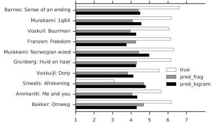
Figure 2: The ten novels with the largest prediction error (using both fragments and bigrams).

Novel	residual
(true - pred.)	mean sent. len.	% direct speech	% Top 3000 vocab.	bzip2 ratio
Rosenboom: Zoete mond	0.075	23.5	24.7	0.80	0.31
Mortier: Godenslaap	0.705	24.9	25.2	0.77	0.34
Lewinsky: Johannistag	0.100	18.3	28.6	0.85	0.32
Eco: The Prague cemetery	0.148	24.5	15.7	0.79	0.33
Franzen: Freedom	2.154	16.2	56.8	0.84	0.33
Barnes: Sense of an ending	2.143	14.1	23.1	0.85	0.32
Voskuil: Buurman	2.117	7.66	58.0	0.89	0.28
Murakami: 1q84	1.870	12.3	20.4	0.84	0.32

Table 5: Comparison of baseline features for novels with good (1–4) and bad (5–8) predictions.

Figure 2 shows a bar plot of the ten novels with the largest prediction error with the fragment and word bigram models. Of these novels, 9 are highly literary and underestimated by the model. For the other novel (Smeets, Afrekening) the literary rating is overestimated by the model. Since this top 10 is based on the mean prediction from both models, the error is large for both models. This does not change when the top 10 errors using only fragments or bigrams is inspected; i.e., the hardest novels to predict are hard with both feature types.

What could explain these errors? At first sight, there is no obvious commonality between the literary novels that are predicted well, or between the ones with a large error; e.g., whether the novels have been translated or not does not explain the error. A possible explanation is that the successfully predicted literary novels share a particular (e.g., rich) writing style that sets them apart from other novels, while the literary novels that are underestimated by the model are not marked by such a writing style. It is difficult to confirm this directly by inspecting the model, since each prediction is the sum of several thousand features, and the contributions of these features form a long tail. If we define the contribution of a feature as the absolute value of its weight times its relative frequency in the document, then in case of Barnes, The sense of an ending, the top 100 features contribute only 34 % of the total prediction.

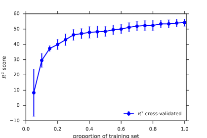
Figure 3: Learning curve when varying training set size. The error bars show the standard error.

Table 5 gives the basic features for the top 4 literary novels with the largest error and contrasts them with 4 literary novels which are well predicted. The most striking difference is sentence length: the underestimated literary novels have markedly shorter sentences. Voskuil and Franzen have a higher proportion of direct speech (they are in fact the only literary novels in the top 10 novels with the most direct speech). Lastly, the underestimated novels have a higher proportion of common words (lower vocabulary richness). These observations are compatible with the explanation suggested above, that a subset of the literary novels share a simple, readable writing style with non-literary novels. Such a style may be more difficult to detect than a literary style with long and complex sentences, or rich vocabulary and phraseology, because a simple, well-crafted sentence may not offer overt surface markers of stylization. Book reviews appear to support this notion for The sense of an ending: “A slow burn, measured but suspenseful, this compact novel makes every slyly crafted sentence count” [Tonkin (2011]; and “polished phrasings, elegant verbal exactness and epigrammatic perceptions” [Kemp (2011].

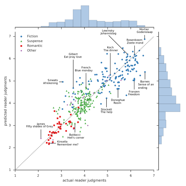
Figure 4: A scatter plot of regression predictions and actual literary ratings. Original/translated titles. Note the histograms beside the axes showing the distribution of ratings (top) and predictions (right).

In order to test whether the amount of data is sufficient to learn to predict the ratings, we construct a learning curve for different training set sizes; cf. Figure 3. The set of novels is shuffled once, so that initial segments of different size represent random samples. The novels are sampled in 5 % increments (i.e., 20 models are trained). The graphs show the cross-validated scores.

The graphs show that increasing the number of novels has a large effect on performance. The curve is steep up to 30 % of the training set, and the performance keeps improving steadily but more slowly up to the last data point. Since the performance is relatively flat starting from 85 %, we can conclude that the $k$-fold cross-validation with $k=5$ provides an adequate estimate of the model’s performance if it were trained on the full dataset; if the model was still gaining performance significantly with more training data, the cross-validation score would underestimate the true prediction performance.

A similar experiment was performed varying the number of features. Here the performance plateaus quickly and reaches an $R^{2}$ of 53.0 % at 40 %, and grows only slightly from that point.

5 Metadata features

In addition to textual features, we also include three (categorical) metadata features not extracted from the text, but still an inherent feature of the novel in question: Genre, Translated, and Author gender; cf. Table 6 for the results. Figure 4 shows a visualization of the predictions in a scatter plot.

Genre is the coarse genre classification Fiction, Suspense, Romantic, Other, derived from the publisher’s categorization. Genre alone is already a strong predictor, with an $R^{2}$ of 58.3 on its own. However, this score is arguably misleading, because the predictions are very coarse due to the discrete nature of the feature.

A striking result is that the variables Author gender and Translated increase the score, but only when they are both present. Inspecting the mean ratings shows that translated novels by female authors have an average rating of 3.8, while originally Dutch male authors are rated 5.0 on average; the ratings of the other combinations lie in between these extremes. This explains why the combination works better than either feature on its own, but due to possible biases inherent in the makeup of the corpus, such as which female or translated authors are published and selected for the corpus, no conclusions on the influence of gender or translation should be drawn from these datapoints.

	$R^{2}$
Basic features (Table 1)	30.0
+ Auto. induced feat. (Table 4)	61.2
+ Genre	74.3
+ Translated	74.0
+ Author gender	76.0

Table 6: Metadata features; incremental scores.

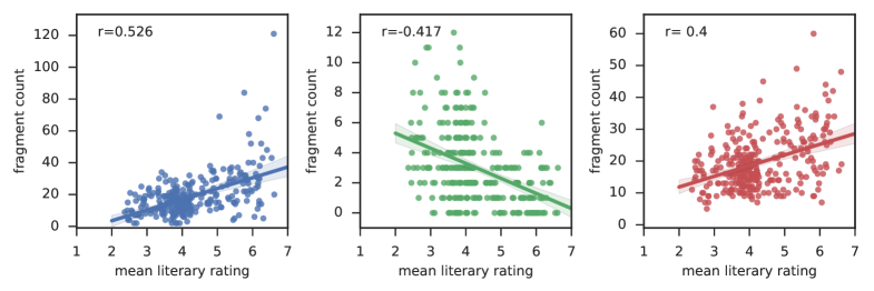
Figure 5: Three fragments whose frequencies in the first fold have a high correlation with the literary ratings. Note the different scales on the $y$-axis. From left to right; Blue: complex NP with comma; Green: quoted speech; Red: Adjunct PP with indefinite article.

6 Previous work

Table 7 shows an overview of previous work on the task of predicting the (literary) quality of novels. Note that the datasets and targets differ, therefore none of the results are directly comparable. For example, regression is a more difficult task than binary classification, and recognizing the difference between an average and highly literary novel is more difficult than distinguishing either from a different domain or genre (e.g., newswire).

?) discriminate literature from other texts using Latent Semantic Analysis. ?) use bigrams, pos tags, and grammar productions to predict the popularity of Gutenberg texts. ?) predict the literary ratings of texts, as in the present paper, but only using bigrams, and on a smaller, less diverse corpus. Compared to previous work, this paper gives a more precise estimate of how well shades of literariness can be predicted from a diverse range of features, including larger and more abstract syntactic constructions.

Binary classification	Dataset, task	Acc.
?)	119 all-time literary classics and 55 other texts, literary novels vs. non-fiction/sci-fi	87.4
?)	800 19th century novels, low vs. high download count	75.7
?)	146 recent novels, low vs. high survey ratings	90.4
Regression result	Dataset, task	$R^{2}$
?)	146 recent novels, survey ratings	61.3
This work	401 recent novels, survey ratings	76.0

Table 7: Overview of previous work on modeling (literary) quality of novels.

fully lexicalized	1,321
syntactic (no lexical items)	2,283
mixed	4,038
discontinuous	684
discontinuous substitution site	396
total	7,642

Table 8: Breakdown of fragment types selected in the first fold.

7 Analysis of selected tree fragments

An advantage of parse tree fragments is that they offer opportunities for interpretation in terms of linguistic aspects as well as basic distributional aspects such as shape and size.

Figure 5 shows three fragments ranked highly by the correlation metric, as extracted from the first fold. The first fragment shows an incomplete constituent, indicated by the ellipses as first and last leaves. Such incomplete fragments are made possible by the binarization scheme (cf. Sec. 4.1).

Table 8 shows a breakdown of fragment types in the first fold. In contrast with $n$-grams, we also see a large proportion of purely syntactic fragments, and fragments mixing both lexical elements and substitution sites. In the case of discontinuous fragments, it turns out that the majority has a positive correlation; this might be due to being associated with more complex constructions.

Figure 6 shows a breakdown by fragment size (defined as number of non-terminals), distinguishing fragments that are positively versus negatively correlated with the literary ratings.

Note that 1 and 3 are special cases corresponding to lexical (e.g., DT $\rightarrow$ the) and binary grammar productions (e.g., NP $\rightarrow$ DT N), respectively. The fragments with 2, 4, and 6 non-terminals are not as common because an even number implies the presence of unary nodes. Except for fragments of size 1, the frontier of fragments can consist of either substitution sites or terminals (since we distinguish only the number of non-terminals). On the one hand smaller fragments corresponding to one or two grammar productions are most common, and are predominantly positively correlated with the literary ratings. On the other hand there is a significant negative correlation between fragment size and literary ratings ($r=-0.2,p<0.001$); i.e., smaller fragments tend to be positively correlated with the literary ratings.

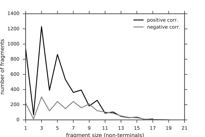
Figure 6: Breakdown by fragment size (number of non-terminals).

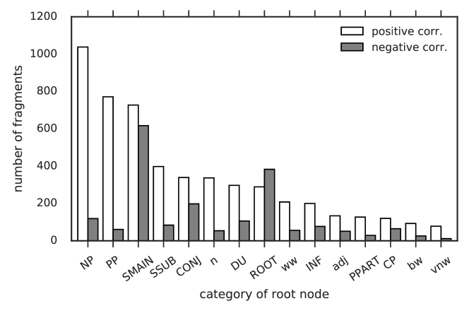
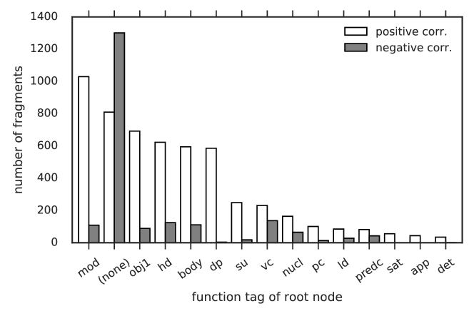
Figure 7: Breakdown by category (above) and function tag (below) of fragment root (top 15 labels).

It is striking that there are more positively than negatively correlated fragments, while literary novels are a minority in the corpus (88 out of 369 novels are rated 5 or higher). Additionally, the breakdown by size shows that the larger number of positively correlated fragments is due to a large number of small fragments of size 3 and 5; however, combinatorially, the number of possible fragment types grows exponentially with size (as reflected in the initial set of recurring fragments), so larger fragment types would be expected to be more numerous. In effect, the selected negatively correlated fragments ignore this distribution by being relatively uniform with respect to size, while the literary fragments actually show the opposite distribution.

What could explain the peak of positively correlated, small fragments? In order to investigate the peak of small fragments, we inspect the 40 fragments of size 3 with the highest correlations. These fragments contain indicators of unusual or more complex sentence structure:

• DU, dp: discourse phenomena for which no specific relation can be assigned (e.g., discourse relations beyond the sentence level).

• appositive NPs, e.g., ‘John the artist.’

• a complex NP, e.g., containing punctuation, nested NPs, or PPs.

• an NP containing an adjective used nominally or an infinitive verb.

On the other hand, most non-literary fragments are top-level productions containing ROOT or clause-level labels, for example to introduce direct speech.

Another way of analyzing the selected fragments is by frequency. When we consider the total frequencies of selected fragments across the corpus, there is a range of 50 to 107,270. The bulk of fragments have a low frequency (before fragment selection 2 is by far the most dominant frequency), but the tail is very long. Except for the fact that there is a larger number of positively correlated fragments, the histograms have a very similar shape.

Lastly, Figure 7 shows a breakdown by the syntactic categories and function tags of the root node of the fragments. The positively correlated fragments are spread over a larger variety of both syntactic categories and function tags. This means that for most labels, the number of positively correlated fragments is higher; the exceptions are ROOT, SV1 (a verb-initial phrase, not part of the top 15), and the absence of a function tag (indicative of a non-terminal directly under the root node). All of these exceptions point to a tendency for negatively correlated fragments to represent templates of complete sentences.

8 Conclusion

The answer to the main research question is that literary judgments are non-arbitrary and can be explained to a large extent from the text itself: there is an intrinsic literariness to literary texts. Our model employs an ensemble of textual features that show a cumulative improvement on predictions, achieving a total score of 76.0 % variation explained. This result is remarkably robust: not just broad genre distinctions, but also finer distinctions in the ratings are predicted.

The experiments showed one clear pattern: literary language tends to use a larger set of syntactic constructions than the language of non-literary novels. This also provides evidence for the hypothesis that literature employs a specific inventory of constructions. All evidence points to a notion of literature which to a substantial extent can be explained purely from internal, textual factors, rather than being determined by external, social factors.

Code and details of the experimental setup are available at https://github.com/andreasvc/literariness

References

- Ashok et al. (2013 Vikas Ashok, Song Feng, and Yejin Choi. 2013. Success with style: using writing style to predict the success of novels. In Proceedings of EMNLP, pages 1753–1764. http://aclweb.org/anthology/D13-1181.
- Baldick (2008 Chris Baldick. 2008. Literariness. In The Oxford Dictionary of Literary Terms. Oxford University Press, USA.
- Bergsma et al. (2012 Shane Bergsma, Matt Post, and David Yarowsky. 2012. Stylometric analysis of scientific articles. In Proceedings of NAACL, pages 327–337. http://aclweb.org/anthology/N12-1033.
- Blei et al. (2003 David M. Blei, Andrew Y. Ng, and Michael I. Jordan. 2003. Latent Dirichlet allocation. the Journal of machine Learning research, 3:993–1022. http://www.jmlr.org/papers/volume3/blei03a/blei03a.pdf.
- Bod (1992 Rens Bod. 1992. A computational model of language performance: Data-oriented parsing. In Proceedings COLING, pages 855–859. http://aclweb.org/anthology/C92-3126.
- Bouma et al. (2001 Gosse Bouma, Gertjan van Noord, and Robert Malouf. 2001. Alpino: Wide-coverage computational analysis of Dutch. Language and Computers, 37(1):45–59. http://www.let.rug.nl/vannoord/papers/alpino.pdf.
- Bourdieu (1996 Pierre Bourdieu. 1996. The rules of art: Genesis and structure of the literary field. Stanford University Press.
- Collins and Duffy (2002 Michael Collins and Nigel Duffy. 2002. New ranking algorithms for parsing and tagging: Kernels over discrete structures, and the voted perceptron. In Proceedings of ACL. http://aclweb.org/anthology/P02-1034.
- Covington et al. (2006 Michael A. Covington, Congzhou He, Cati Brown, Lorina Naci, and John Brown. 2006. How complex is that sentence? A proposed revision of the Rosenberg and Abbeduto D-Level scale. CASPR Research Report 2006-01, Artificial Intelligence Center.
- Flesch (1948 Rudolph Flesch. 1948. A new readability yardstick. Journal of applied psychology, 32(3):221.
- Gibson (2000 Edward Gibson. 2000. The dependency locality theory: A distance-based theory of linguistic complexity. Image, language, brain, pages 95–126.
- Harris (1995 Wendell V. Harris. 1995. Literary meaning. Reclaiming the study of literature. Palgrave Macmillan, London.
- Jautze et al. (2016 Kim Jautze, Andreas van Cranenburgh, and Corina Koolen. 2016. Topic modeling literary quality. In Digital Humanities 2016: Conference Abstracts, pages 233–237, Krákow, Poland. http://dh2016.adho.org/abstracts/95.
- Kemp (2011 Peter Kemp. 2011. The sense of an ending by Julian Barnes. Book review, The Sunday Times, July 24. http://www.thesundaytimes.co.uk/sto/culture/books/fiction/article674085.ece.
- Kim et al. (2011 Sangkyum Kim, Hyungsul Kim, Tim Weninger, and Jiawei Han. 2011. Authorship classification: A syntactic tree mining approach. In Proceedings of SIGIR, pages 455–464. ACM. http://dx.doi.org/10.1145/2009916.2009979.
- Klein and Manning (2003 Dan Klein and Christopher D. Manning. 2003. Accurate unlexicalized parsing. In Proceedings of ACL, volume 1, pages 423–430. http://aclweb.org/anthology/P03-1054.
- Louwerse et al. (2008 Max Louwerse, Nick Benesh, and Bin Zhang. 2008. Computationally discriminating literary from non-literary texts. In S. Zyngier, M. Bortolussi, A. Chesnokova, and J. Auracher, editors, Directions in empirical literary studies: In honor of Willie Van Peer, pages 175–191. John Benjamins Publishing Company, Amsterdam.
- McDonald (2007 Ronan McDonald. 2007. The death of the critic. Continuum, London.
- Moschitti (2006 Alessandro Moschitti. 2006. Making tree kernels practical for natural language learning. In Proceedings of EACL, pages 113–120. http://aclweb.org/anthology/E06-1015.
- Oostdijk et al. (2013 Nelleke Oostdijk, Martin Reynaert, Véronique Hoste, and Ineke Schuurman. 2013. The construction of a 500-million-word reference corpus of contemporary written dutch. In Essential speech and language technology for Dutch, pages 219–247. Springer.
- Sangati et al. (2010 Federico Sangati, Willem Zuidema, and Rens Bod. 2010. Efficiently extract recurring tree fragments from large treebanks. In Proceedings of LREC, pages 219–226. http://dare.uva.nl/record/371504.
- Scha (1990 Remko Scha. 1990. Language theory and language technology; competence and performance. In Q.A.M. de Kort and G.L.J. Leerdam, editors, Computertoepassingen in de Neerlandistiek, pages 7–22. LVVN, Almere, the Netherlands. Original title: Taaltheorie en taaltechnologie; competence en performance. English translation: http://iaaa.nl/rs/LeerdamE.html.
- Stamatatos (2006 Efstathios Stamatatos. 2006. Ensemble-based author identification using character n-grams. In Proceedings of the 3rd International Workshop on Text-based Information Retrieval, pages 41–46. http://ceur-ws.org/Vol-205/paper8.pdf.
- Stamatatos (2009 Efstathios Stamatatos. 2009. A survey of modern authorship attribution methods. Journal of the American Society for Information Science and Technology, 60(3):538–556. http://dx.doi.org/10.1002/asi.21001.
- Swanson and Charniak (2012 Benjamin Swanson and Eugene Charniak. 2012. Native language detection with tree substitution grammars. In Proceedings of ACL, pages 193–197. http://aclweb.org/anthology/P12-2038.
- Swanson and Charniak (2013 Ben Swanson and Eugene Charniak. 2013. Extracting the native language signal for second language acquisition. In Proceedings of NAACL-HLT, pages 85–94. http://aclweb.org/anthology/N13-1009.
- Tonkin (2011 Boyd Tonkin. 2011. The sense of an ending, by Julian Barnes. Book review, The Independent, August 5. http://www.independent.co.uk/arts-entertainment/books/reviews/the-sense-of-an-ending-by-julian-barnes-2331767.html.
- van Cranenburgh and Koolen (2015 Andreas van Cranenburgh and Corina Koolen. 2015. Identifying literary texts with bigrams. In Proc. of workshop Computational Linguistics for Literature, pages 58–67. http://aclweb.org/anthology/W15-0707.
- van Cranenburgh (2012 Andreas van Cranenburgh. 2012. Literary authorship attribution with phrase-structure fragments. In Proceedings of CLFL, pages 59–63. Revised version: http://andreasvc.github.io/clfl2012.pdf.
- van Cranenburgh (2014 Andreas van Cranenburgh. 2014. Extraction of phrase-structure fragments with a linear average time tree kernel. Computational Linguistics in the Netherlands Journal, 4:3–16. http://www.clinjournal.org/sites/default/files/01-Cranenburgh-CLIN2014.pdf.
- van Eynde (2005 Frank van Eynde. 2005. Part of speech tagging en lemmatisering van het D-COI corpus. Transl.: POS tagging and lemmatization of the D-COI corpus, tech report, July 2005. http://www.ccl.kuleuven.ac.be/Papers/DCOIpos.pdf.
- van Wingerden and Hendriks (2015 Wouter van Wingerden and Pepijn Hendriks. 2015. Dat Hoor Je Mij Niet Zeggen: De allerbeste taalclichés. Thomas Rap, Amsterdam. Transl.: You didn’t hear me say that: The very best linguistic clichés.
- Yu and Liu (2004 Lei Yu and Huan Liu. 2004. Efficient feature selection via analysis of relevance and redundancy. Journal of Machine Learning Research, 5:1205–1224. http://jmlr.org/papers/volume5/yu04a/yu04a.pdf.