Central limit theorem for the Horton-Strahler bifurcation ratio of general branch order

Abstract

Abstract
The Horton-Strahler ordering method, originating in hydrology, formulates the hierarchical structure of branching patterns using a quantity called the bifurcation ratio. The main result of this paper is the central limit theorem for bifurcation ratio of general branch order. This is a generalized form of the central limit theorem for the lowest bifurcation ratio, which was previously proved. Some useful relations are also derived in the proofs of the main theorems.

1 Introduction

Branching objects are found very widely Ball , ranging from natural patterns like river networks, plants, and dendritic crystals, to conceptual expressions like binary search trees in computer science Knuth and phylogenetic trees in taxonomy Archibald . The topological structure of a branching pattern is modeled by a binary tree if a segment bifurcates (does not trifurcate or more) at every branching point.

Let $\Omega_{n}$ denote the set of the different binary trees having $n$ leaves. The number of leaves is called the magnitude in research of branching patterns. As known well Stanley , the number of the different binary trees of magnitude $n$ is given by

$$|\Omega_{n}|=\frac{1}{2n-1}\binom{2n-1}{n}=\frac{(2n-2)!}{n!(n-1)!},$$

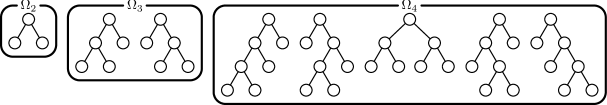
which iscalled the $n-1$st Catalan number. In Fig. 1, $\Omega_{n}$ for $n=2,3$, and 4 are schematically shown. Introducing the uniform probability measure $P_{n}$ on $\Omega_{n}$ (so that each binary tree is assigned equal probability $1/|\Omega_{n}|$), we obtain the probability space $(\Omega_{n},P_{n})$ referred to as the random model Shreve . The formation of real-world branching patterns more or less involves stochastic effects, and the random model is a kind of mathematical simplification of such random factors.

In hydrology, methods for measuring the hierarchical structure of a river network have been proposed by Horton Horton , Strahler Strahler , Shreve Shreve , Tokunaga Tokunaga , and other researchers. Their methods define how to assign an integer number (called the order) to each stream. Among all, Strahler’s method is currently the most popular because of its simple computation rule. Strahler’s method is a refinement of Horton’s method, so it is sometimes called the Horton-Strahler ordering method. The Horton-Strahler method recursively defines the order of each node by the following rules. (i) The leaf nodes are defined to have order one. (ii) A node whose children have different order $r_{1}$ and $r_{2}$ ($r_{1}\neq r_{2}$) has order $\max\{r_{1},r_{2}\}$. (iii) A node whose two children have the same order $r$ has order $r+1$. We define a branch of order $r$ as a maximal connected path made by nodes of equal order $r$. (A branch here is called a stream in the analysis of river networks.) An example of Strahler’s ordering is shown in Fig. 2. For a binary tree $\tau\in\Omega_{n}$, we let $S_{r,n}(\tau)$ denote the number of branches of order $r$ in $\tau$. By the definition of the order, $S_{1,n}(\tau)=n$ and $0\leq S_{r,n}(\tau)\leq n/2^{r-1}$ ($r\geq 2$). Note that $S_{2,n}(\tau)\neq 0$ if $n\geq 2$, because a node of order 2 is produced by the merge of two leaves. For the binary tree $\tau(\in\Omega_{6})$ in Fig. 2, $S_{1,6}(\tau)=6$, $S_{2,6}(\tau)=2$, $S_{3,6}(\tau)=1$, and $S_{r,6}(\tau)=0$ for $r\geq 4$. $S_{r,n}$ is a random variable on $(\Omega_{n},P_{n})$, and its stochastic property is of main interest in this study.

Figure 1: $\Omega_{2},\Omega_{3}$, and $\Omega_{4}$ contain one, two, and five binary trees, respectively.

Figure 2: A small example of ordering and branches. The number on each node represents the order of the node. The branches of order 2 and 3 are shown by the dashed rectangles. This binary tree consists of six branches of order 1, two branches order 2, and one branch of order 3.

For any function $f:\{0,1,2,\ldots\}\to\mathbb{R}$, $f(S_{r,n}(\cdot))$ is a real-valued random variable on $\Omega_{n}$. According to Ref. Yamamoto2010 , the recursive relation between the averages of the $r$th and $r-1$st variables

$$E\left[f(S_{r,n})\right]=\frac{n!(n-1)!(n-2)!}{(2n-2)!}\sum_{m=1}^{\lfloor n/2\rfloor}\frac{2^{n-2m}}{(n-2m)!m!(m-1)!}E\left[f(S_{r-1,m})\right]$$ (1)

holds, where $E\left[\cdot\right]$ denotes the average on the random model. The coefficient

$$\frac{n!(n-1)!(n-2)!2^{n-2m}}{(2n-2)!(n-2m)!m!(m-1)!}$$

represents the probability $P_{n}(S_{2,n}=m)$. In particular, putting $r=2$ in Eq. (1), we have

$$E\left[f(S_{2,n})\right]=\frac{n!(n-1)!(n-2)!}{(2n-2)!}\sum_{m=1}^{\lfloor n/2\rfloor}\frac{2^{n-2m}}{(n-2m)!m!(m-1)!}f(m).$$ (2)

Mathematical properties of $S_{2,n}$ have been investigated thoroughly. For instance, the average and variance are respectively given by Werner

$$E\left[S_{2,n}\right]=\frac{n(n-1)}{2(2n-3)},\quad\operatorname{Var}\left[S_{2,n}\right]=\frac{n(n-1)(n-2)(n-3)}{2(2n-3)^{2}(2n-5)}.$$ (3)

Moreover, from Eq. (2), the moment generating function $M_{2,n}(t)$ of $S_{2,n}$ is given by

$$M_{2,n}(t):=E\left[\exp(S_{2,n}t)\right]=\frac{n!(n-1)!(n-2)!}{(2n-2)!}\sum_{m=1}^{\lfloor n/2\rfloor}\frac{2^{n-2m}}{(n-2m)!m!(m-1)!}e^{mt},$$

and this summation can be expressed using the Gauss hypergeometric function $F$ Yamamoto2008 :

$$M_{2,n}(t)=\frac{2^{n-2}n!(n-1)!}{(2n-2)!}e^{t}F\left(\frac{2-n}{2},\frac{3-n}{2},2;e^{t}\right).$$ (4)

The ratio $S_{r+1,n}(\tau)/S_{r,n}(\tau)$ is called the bifurcation ratio of order $r$ or simply the $r$th bifurcation ratio. Hydrologists have empirically confirmed that the bifurcation ratios of an actual river network become almost constant for different orders, and this relation is referred to as Horton’s law of stream numbers. By definition, the bifurcation ratio is always smaller than or equal to $1/2$. When $S_{r,n}(\tau)=0$, we reasonably define $S_{r+1,n}(\tau)/S_{r,n}(\tau)=0$. The random variable $S_{r+1,n}/S_{r,n}$ is also called the $r$the bifurcation ratio. The lowest bifurcation ratio $S_{2,n}/S_{1,n}=S_{2,n}/n$ is relatively easy to deal with, because it is similar to $S_{2,n}$. The central limit theorem for $S_{2,n}/n$ has been shown by Wang and Waymire Wang :

Theorem 1 (Central limit theorem for the lowest bifurcation ratio).

On the random model,

$$\sqrt{n}\left(\frac{S_{2,n}}{n}-\frac{1}{4}\right)\Rightarrow N\left(0,\frac{1}{16}\right),\quad n\to\infty,$$

where “$\Rightarrow$” denotes convergence in distribution, and $N(\mu,\sigma^{2})$ is the normal distribution with mean $\mu$ and variance $\sigma^{2}$.

It is a simple and natural idea that we extend Theorem 1 to general order $r$. Compared with $S_{2,n}$, however, higher-order branches $S_{r,n}$ for $r\geq 3$ and the bifurcation ratio of order $r\geq 2$ is difficult to handle and less studied. In this paper, we generalize Theorem 1 in two ways (Theorems 2 and 3 in §2), and further generalize them (Theorem 4 in §6). In §3–5, we give proofs of lemmas, which are necessary for the main theorems. In these proofs, Eq. (1) and its variant

$$E\left[f\left(\frac{S_{r+1,n}}{S_{r,n}}\right)\right]=\frac{n!(n-1)!(n-2)!}{(2n-2)!}\sum_{m=1}^{\lfloor n/2\rfloor}\frac{2^{n-2m}}{(n-2m)!m!(m-1)!}E\left[f\left(\frac{S_{r,m}}{S_{r-1,m}}\right)\right].$$ (5)

are very useful.

2 Main results

The following two theorems are the main results of the present paper.

Theorem 2 (Central limit theorem for the bifurcation ratio of general order).

For any order $r=1,2,3,\ldots$, the $r$th bifurcation ratio $S_{r+1,n}/S_{r,n}$ satisfies

$$\sqrt{n}\left(\frac{S_{r+1,n}}{S_{r,n}}-\frac{1}{4}\right)\Rightarrow N\left(0,4^{r-3}\right),\quad n\to\infty,$$ (6)

Theorem 3 (Central limit theorem for the number of branches of general order).

For any order $r=1,2,3,\ldots$, the number $S_{r+1,n}$ of $r+1$st branches satisfies

$$\sqrt{n}\left(\frac{S_{r+1,n}}{n}-\frac{1}{4^{r}}\right)\Rightarrow N\left(0,\frac{1}{3}\frac{4^{r}-1}{16^{r}}\right),\quad n\to\infty,$$ (7)

Remark.

These two theorems are generalization of Theorem 1 to general order $r$; they are reduced to Theorem 1 by setting $r=1$. Theorem 2 states the property of the bifurcation ratio $S_{r+1,n}/S_{r,n}$, and Theorem 3 states the property of the number of branches $S_{r+1,n}$. The limit variance $4^{r-3}$ in Theorem 2 becomes large as $r$ increases, whereas the limit variance in Theorem 3 becomes small as $r$ increases.

From Theorem 2, the following property, which can be regarded as Horton’s law of stream numbers, is easily derived.

Corollary 1 (Horton’s law of stream numbers for the random model).

For any order $r=1,2,\ldots$, the $r$th bifurcation ratio $S_{r+1,n}/S_{r,n}$ converges in probability to the common value $1/4$:

$$\frac{S_{r+1,n}}{S_{r,n}}\xrightarrow{p}\frac{1}{4},$$

where “$\xrightarrow{p}$” denotes convergence in probability.

Let us introduce the asymptotic equality, since this study mainly focuses on the asymptotic behavior (the limit $n\to\infty$) of $S_{r,n}$.

Definition 1.

The average value $E\left[f(S_{r,n})\right]$ is asymptotically equivalent to $g_{r}(n)$ if

$$\lim_{n\to\infty}\frac{E\left[f(S_{r,n})\right]}{g_{r}(n)}=1,$$

and this is denoted by

$$E\left[f(S_{r,n})\right]\sim g_{r}(n).$$

For example, from Eq. (3),

$$E\left[S_{2,n}\right]=\frac{n(n-1)}{2(2n-3)}\sim\frac{n}{4}.$$

Theorems 2 and 3 are easily proved by using the following Lemmas 1 and 2, respectively.

Lemma 1.

For $r=1,2,\ldots$ and $s=0,1,2,\ldots$,

$$E\left[\left(\frac{S_{r+1,n}}{S_{r,n}}-\frac{1}{4}\right)^{2s}\right]\sim\frac{(2s-1)!!}{4^{2s}}\left(\frac{n}{4^{r-1}}\right)^{-s},\quad E\left[\left(\frac{S_{r+1,n}}{S_{r,n}}-\frac{1}{4}\right)^{2s+1}\right]\sim\frac{(2s+1)!!}{2\cdot 4^{2s+1}}\left(\frac{n}{4^{r-1}}\right)^{-s-1}$$

Lemma 2.

For $r=1,2,\ldots$ and $s=0,1,2,\ldots$,

$$E\left[\left(S_{r+1,n}-\frac{n}{4^{r}}\right)^{2s}\right] \sim\frac{(2s-1)!!}{4^{2sr}}\left(\frac{4^{r}-1}{3}\right)^{s}n^{s},$$

$$E\left[\left(S_{r+1,n}-\frac{n}{4^{r}}\right)^{2s+1}\right] \sim\frac{(2s+1)!!}{2\cdot 4^{(2s+1)r}}\left(\frac{4^{r}-1}{3}\right)^{s}\frac{1}{5}\left(\frac{4^{r+1}-1}{3}+\frac{4^{r-1}-1}{3}4(2s+1)\right)n^{s}.$$

The odd-power result has a more complicated form than the even-power one.

Proof of Theorem 2.

We let $\varphi_{r,n}^{r+1}(z)$ denote the characteristic function of the left-hand side of Eq. (6), where the subscript $r$ and superscript $r+1$ respectively correspond to $S_{r,n}$ in the denominator and $S_{r+1,n}$ in the numerator in Eq. (6). By definition, $\varphi_{r,n}^{r+1}(z)$ is calculated as

$$\varphi_{r,n}^{r+1}(z) =E\left[\exp\left(iz\sqrt{n}\left(\frac{S_{r+1,n}}{S_{r,n}}-\frac{1}{4}\right)\right)\right]$$

$$=E\left[\sum_{k=0}^{\infty}\frac{(iz\sqrt{n})^{k}}{k!}\left(\frac{S_{r+1,n}}{S_{r,n}}-\frac{1}{4}\right)^{k}\right]$$

$$=\sum_{k=0}^{\infty}\frac{(iz\sqrt{n})^{k}}{k!}E\left[\left(\frac{S_{r+1,n}}{S_{r,n}}-\frac{1}{4}\right)^{k}\right]$$

$$=\sum_{s=0}^{\infty}\frac{(iz\sqrt{n})^{2s}}{(2s)!}E\left[\left(\frac{S_{r+1,n}}{S_{r,n}}-\frac{1}{4}\right)^{2s}\right]+\sum_{s=0}^{\infty}\frac{(iz\sqrt{n})^{2s+1}}{(2s+1)!}E\left[\left(\frac{S_{r+1,n}}{S_{r,n}}-\frac{1}{4}\right)^{2s+1}\right],$$

where $i=\sqrt{-1}$. At the last equality, we have split the sum into even $k$ ($k=2s$) and odd $k$ ($k=2s+1$). By Lemma 1, the terms of the first sum (even $k$) are $O(n^{0})$, whereas the terms of the second sum (odd $k$) are $o(n^{0})$. Hence, the second sum can be neglected in the limit $n\to\infty$, so that

$$\varphi_{r,n}^{r+1}(z) \sim\sum_{s=0}^{\infty}\frac{(iz\sqrt{n})^{2s}}{(2s)!}E\left[\left(\frac{S_{r+1,n}}{S_{r,n}}-\frac{1}{4}\right)^{2s}\right]$$

$$\sim\sum_{s=0}^{\infty}\frac{(-z^{2}n)^{s}}{(2s)!}\frac{(2s-1)!!}{4^{2s}}\frac{n^{-s}}{4^{-(r-1)s}}$$

$$=\sum_{s=0}^{\infty}\left(-\frac{4^{r-3}z^{2}}{2}\right)^{s}\frac{1}{s!}$$

$$=\exp\left(-\frac{4^{r-3}z^{2}}{2}\right).$$

Recall that the characteristic function of $N(\mu,\sigma^{2})$ is $\exp(i\mu z-\sigma^{2}z^{2}/2)$. Since $\varphi_{r,n}^{r+1}$ converges pointwise to the characteristic function of $N(0,4^{r-3})$, convergence in distribution in Theorem 2 is proved. (For the properties of a characteristic function, see Feller Feller for example.)

Keep in mind that the neglect of the odd-power terms is a crucial point also in the other central limit theorems in this paper. ∎

Proof of Theorem 3.

As with the above proof of Theorem 2, the characteristic function $\varphi_{1,n}^{r+1}(z)$ of the left-hand side of Eq. (7) is

$$\varphi_{1,n}^{r+1}(z) =E\left[\exp\left(iz\sqrt{n}\left(\frac{S_{r+1,n}}{n}-\frac{1}{4^{r}}\right)\right)\right]$$

$$=\sum_{k=0}^{\infty}\frac{(iz\sqrt{n})^{k}}{k!}E\left[\left(\frac{S_{r+1,n}}{n}-\frac{1}{4^{r}}\right)^{k}\right]$$

$$=\sum_{s=0}^{\infty}\frac{(iz\sqrt{n})^{2s}}{(2s)!n^{2s}}E\left[\left(S_{r+1,n}-\frac{n}{4^{r}}\right)^{2s}\right]+\sum_{s=0}^{\infty}\frac{(iz\sqrt{n})^{2s+1}}{(2s+1)!n^{2s+1}}E\left[\left(S_{r+1,n}-\frac{n}{4^{r}}\right)^{2s+1}\right].$$

By Lemma 2, the second sum is neglected and the dominant terms are calculated to

$$\varphi_{1,n}^{r+1}(z) \sim\sum_{s=0}^{\infty}\frac{(iz\sqrt{n})^{2s}}{(2s)!n^{2s}}E\left[\left(S_{r+1,n}-\frac{n}{4^{r}}\right)^{2s}\right]$$

$$\sim\sum_{s=0}^{\infty}\frac{(-z^{2}n)^{s}}{(2s)!n^{2s}}\frac{(2s-1)!!}{4^{2rs}}\left(\frac{4^{r}-1}{3}\right)^{s}n^{s}$$

$$=\sum_{s=0}^{\infty}\left(-\frac{z^{2}}{2}\frac{4^{r}-1}{3\cdot 16^{r}}\right)^{s}\frac{1}{s!}$$

$$=\exp\left(-\frac{z^{2}}{2}\frac{4^{r}-1}{3\cdot 16^{r}}\right).$$

Therefore, the converges in distribution to $N(0,(4^{r}-1)/(3\cdot 16^{r}))$ is proved. ∎

We give the proofs of Lemmas 1 and 2 in the following three sections.

3 Starting point of Lemmas 1 and 2

We show Lemmas 1 and 2 by induction on $r$. In this section, the case of $r=1$ in Lemmas 1 and 2 is proved (Cor. 3).

Proposition 1.

For a two-variable polynomial $p(\cdot,\cdot)$ of finite degree,

$$E\left[S_{2,n}p(S_{2,n},n)\right]=\frac{n}{2}E\left[p(S_{2,n},n)\right]-\frac{n(n-2)}{2(2n-3)}E\left[p(S_{2,n-1},n)\right].$$ (8)

Here, $E\left[S_{2,n}p(S_{2,n},n)\right]$ and $E\left[p(S_{2,n},n)\right]$ are taken over $\Omega_{n}$, whereas $E\left[p(S_{2,n-1},n)\right]$ are over $\Omega_{n-1}$.

Proof.

Because of the linearity of $E\left[\cdot\right]$, it is sufficient to check the case $p(S_{2,n},n)=S_{2,n}^{k}n^{l}$. The average is expressed using the moment generating function $M_{2,n}(t)$ in Eq. (4).

$$E\left[S_{2,n}S_{2,n}^{k}n^{l}\right] =n^{l}E\left[S_{2,n}^{k+1}\right]=n^{l}\left.\frac{d^{k+1}}{dt^{k+1}}M_{2,n}(t)\right|_{t=0}$$

$$=n^{l}\frac{2^{n-2}n!(n-1)!}{(2n-2)!}\left.\frac{d^{k+1}}{dt^{k+1}}e^{t}F\left(\frac{2-n}{2},\frac{3-n}{2},2;e^{t}\right)\right|_{t=0}$$

$$=n^{l}\frac{2^{n-2}n!(n-1)!}{(2n-2)!}\left.\frac{d^{k}}{dt^{k}}e^{t}\left[F\left(\frac{2-n}{2},\frac{3-n}{2},2;e^{t}\right)+\frac{d}{dt}F\left(\frac{2-n}{2},\frac{3-n}{2},2;e^{t}\right)\right]\right|_{t=0}.$$

Using the derivative of the Gauss hypergeometric function Abramowitz

$$\frac{d}{dz}F\left(\alpha,\beta,\gamma;z\right)=\frac{\alpha}{z}[F\left(\alpha+1,\beta,\gamma;z\right)-F\left(\alpha,\beta,\gamma;z\right)]$$

and the symmetry $F\left(\alpha,\beta,\gamma;z\right)=F\left(\beta,\alpha,\gamma;z\right)$, we have

$$\frac{d}{dt}F\left(\frac{2-n}{2},\frac{3-n}{2},2;e^{t}\right)=\frac{n-2}{2}\left[F\left(\frac{2-n}{2},\frac{3-n}{2},2;e^{t}\right)-F\left(\frac{3-n}{2},\frac{4-n}{2},2;e^{t}\right)\right],$$ (9)

thereby

$$E\left[S_{2,n}S_{2,n}^{k}n^{l}\right] =n^{l}\frac{2^{n-2}n!(n-1)!}{(2n-2)!}\frac{d^{k}}{dt^{k}}e^{t}\left[\frac{n}{2}F\left(\frac{2-n}{2},\frac{3-n}{2},2;e^{t}\right)-\frac{n-2}{2}F\left(\frac{3-n}{2},\frac{4-n}{2},2;e^{t}\right)\right]$$

$$=n^{l}\left(\frac{n}{2}E\left[S_{2,n}^{k}\right]-\frac{2n(n-1)}{(2n-2)(2n-3)}\frac{n-2}{2}E\left[S_{2,n-1}^{k}\right]\right)$$

$$=\frac{n}{2}E\left[S_{2,n}^{k}n^{l}\right]-\frac{n(n-2)}{2(2n-3)}E\left[S_{2,n-1}^{k}n^{l}\right].$$

∎

Here we comment on the utility of Prop. 1. We can calculate the moments $E\left[S_{2,n}^{k}\right]$ recursively using Eq. (8):

$$E\left[S_{2,n}\right] =E\left[S_{2,n}\cdot 1\right]=\frac{n}{2}E\left[1\right]-\frac{n(n-2)}{2(2n-3)}E\left[1\right]=\frac{n(n-1)}{2(2n-3)},$$

$$E\left[S_{2,n}^{2}\right] =E\left[S_{2,n}S_{2,n}\right]=\frac{n}{2}E\left[S_{2,n}\right]-\frac{n(n-1)}{2(2n-3)}E\left[S_{2,n-1}\right]=\frac{n(n-1)(n^{2}-n-4)}{4(2n-3)(2n-5)},$$

$$E\left[S_{2,n}^{3}\right] =E\left[S_{2,n}S_{2,n}^{2}\right]=\frac{n}{2}E\left[S_{2,n}^{2}\right]-\frac{n(n-1)}{2(2n-3)}E\left[S_{2,n-1}^{2}\right]=\frac{n(n-1)(n^{4}-2n^{3}-15n^{2}+32n+8)}{8(2n-3)(2n-5)(2n-7)},$$

and so on. The first and second moments were individually calculated Werner (see Eq. (3)). Note, however, that Prop. 1 provides a systematic calculation method of the $k$th moment of $S_{2,n}$ in a bottom-up way. Furthermore, we easily obtain $E\left[S_{2,n}^{k}\right]\sim(n/4)^{k}$ for $k=0,1,2,\ldots$ using Eq. (8).

Corollary 2.

Subtracting $nE\left[p(S_{2,n},n)\right]/4$ from Eq. (8), we have

$$E\left[\left(S_{2,n}-\frac{n}{4}\right)p(S_{2,n},n)\right]=\frac{n}{4}E\left[p(S_{2,n},n)\right]-\frac{n(n-2)}{2(2n-3)}E\left[p(S_{2,n-1},n)\right].$$

Lemma 3.

For $k=0,1,2,\ldots$,

$$E\left[\left(S_{2,n}-\frac{n}{4}\right)^{k}\right]\sim\frac{k!}{2^{\lfloor(k+1)/2\rfloor}\lfloor k/2\rfloor!4^{k}}n^{\lfloor k/2\rfloor}.$$

That is to say, the asymptotic form of $E\left[(S_{2,n}-n/4)^{k}\right]$ depends on whether $k$ is even or odd:

$$E\left[\left(S_{2,n}-\frac{n}{4}\right)^{2s}\right]\sim\frac{(2s-1)!!}{4^{2s}}n^{s},\quad E\left[\left(S_{2,n}-\frac{n}{4}\right)^{2s+1}\right]\sim\frac{(2s+1)!!}{2\cdot 4^{2s+1}}n^{s},$$ (10)

for $s=0,1,2,\ldots$.

Remark.

In $E\left[S_{2,n}-n/4\right]$ ($k=1$), the leading $O(n^{1})$ terms are canceled because of $E\left[S_{2,n}\right]\sim n/4$. Similarly, in general $k$, $O(n^{k}),O(n^{k-1}),\ldots$ terms are successively canceled, so that the resultant leading order of $E\left[(S_{2,n}-n/4)^{k}\right]$ becomes $\lfloor k/2\rfloor$. This effect makes the estimation of $E\left[(S_{2,n}-n/4)^{k}\right]$ difficult.

Proof.

The proof is by induction on $k$. The statement is true for $k=0,1$, and 2, because

$$E\left[\left(S_{2,n}-\frac{n}{4}\right)^{0}\right] =1,$$

$$E\left[\left(S_{2,n}-\frac{n}{4}\right)^{1}\right] =\frac{n(n-1)}{2(2n-3)}-\frac{n}{4}=\frac{n}{4(2n-3)}\sim\frac{1}{8},$$

$$E\left[\left(S_{2,n}-\frac{n}{4}\right)^{2}\right] =E\left[S_{2,n}^{2}\right]-\frac{n}{2}E\left[S_{2,n}\right]+\frac{n^{2}}{16}=\frac{n(4n^{2}-17n+16)}{16(2n-3)(2n-5)}\sim\frac{n}{16}.$$

Assume that it is true up to $k\geq 2$, and we show it is true for $k+1$. It follows from Cor. 2 that

$$E\left[\left(S_{2,n}-\frac{n}{4}\right)^{k+1}\right] =E\left[\left(S_{2,n}-\frac{n}{4}\right)\left(S_{2,n}-\frac{n}{4}\right)^{k}\right]$$

$$=\frac{n}{4}E\left[\left(S_{2,n}-\frac{n}{4}\right)^{k}\right]-\frac{n(n-2)}{2(2n-3)}E\left[\left(S_{2,n-1}-\frac{n}{4}\right)^{k}\right]$$

$$=\frac{n}{4}E\left[\left(S_{2,n}-\frac{n}{4}\right)^{k}\right]-\frac{n(n-2)}{2(2n-3)}E\left[\left(S_{2,n-1}-\frac{n-1}{4}-\frac{1}{4}\right)^{k}\right]$$

$$=\frac{n}{4}E\left[\left(S_{2,n}-\frac{n}{4}\right)^{k}\right]-\frac{n(n-2)}{2(2n-3)}\sum_{l=0}^{k}\binom{k}{l}\left(-\frac{1}{4}\right)^{l}E\left[\left(S_{2,n-1}-\frac{n-1}{4}\right)^{k-l}\right].$$

In the following, we separately investigate odd and even $k$.

Case 1: $k$ is odd ($k=2s+1$). The dominant terms are $l=0$ and 1 in the summation, and the others can be neglected. Thus,

$$E\left[\left(S_{2,n}-\frac{n}{4}\right)^{2s+1+1}\right]$$

$$\sim\frac{n}{4}E\left[\left(S_{2,n}-\frac{n}{4}\right)^{2s+1}\right]-\frac{n(n-2)}{2(2n-3)}\left(E\left[\left(S_{2,n-1}-\frac{n-1}{4}\right)^{2s+1}\right]-\frac{2s+1}{4}E\left[\left(S_{2,n-1}-\frac{n-1}{4}\right)^{2s}\right]\right)$$

$$\sim\frac{n}{4}\frac{(2s+1)!!}{4^{2s+1}}-\frac{n}{4}\left(\frac{(2s+1)!!}{4^{2s+1}}(n-1)^{s}-\frac{2s+1}{4}\frac{(2s-1)!!}{4^{2s}}(n-1)^{s}\right)$$

$$\sim\frac{(2s+1)!!}{4^{2s+2}}n^{s+1}.$$

Case 2: $k$ is even ($k=2s$). Picking out the terms up to $O(n^{s})$ carefully, we obtain

$$E\left[\left(S_{2,n}-\frac{n}{4}\right)^{2s+1}\right]$$

$$=\frac{n}{4}E\left[\left(S_{2,n}-\frac{n}{4}\right)^{2s}\right]-\frac{n(n-2)}{2(2n-3)}\left(E\left[\left(S_{2,n-1}-\frac{n-1}{4}\right)^{2s}\right]-\frac{2s}{4}E\left[\left(S_{2,n-1}-\frac{n-1}{4}\right)^{2s-1}\right]\right.$$

$$\qquad\left.+\frac{2s(2s-1)}{16\cdot 2}E\left[\left(S_{2,n-1}-\frac{n-1}{4}\right)^{2s-2}\right]+o(n^{s-1})\right).$$ (11)

We introduce the coefficient $a_{s}$ as

$$E\left[\left(S_{2,n}-\frac{n}{4}\right)^{2s}\right]=\frac{(2s-1)!!}{4^{2s}}n^{s}+a_{s}n^{s-1}+o(n^{s-1}),$$

and expand each term on the right-hand side of Eq. (11) up to $O(n^{s})$ using the induction hypothesis:

$$\frac{n}{4}E\left[\left(S_{2,n}-\frac{n}{4}\right)^{2s}\right] =\frac{(2s-1)!!}{4^{2s+1}}n^{s+1}+\frac{a_{s}}{4}n^{s}+o(n^{s}),$$

$$\frac{n(n-2)}{2(2n-3)}E\left[\left(S_{2,n-1}-\frac{n-1}{4}\right)^{2s}\right] =\frac{(2s-1)!!}{4^{2s+1}}n^{s+1}-\frac{(2s+1)!!}{2\cdot 4^{2s+1}}n^{s}+\frac{a_{s}}{4}n^{s}+o(n^{s}),$$

$$\frac{n(n-2)}{2(2n-3)}\frac{2s}{4}E\left[\left(S_{2,n-1}-\frac{n-1}{4}\right)^{2s-1}\right] =\frac{(2s-1)!!}{4^{2s+1}}sn^{s}+o(n^{s}),$$

$$\frac{n(n-2)}{2(2n-3)}\frac{2s(2s-1)}{16\cdot 2}E\left[\left(S_{2,n-1}-\frac{n-1}{4}\right)^{2s-2}\right] =\frac{(2s-1)!!}{4^{2s+1}}sn^{s}+o(n^{s}).$$

Therefore,

$$E\left[\left(S_{2,n}-\frac{n}{4}\right)^{2s+1}\right]=\frac{(2s+1)!!}{2\cdot 4^{2s+1}}n^{s}+o(n^{s}).$$

Note that $O(n^{s+1})$ terms and those including $a_{s}$ are all cancelled.

Therefore, the statement is true for any $k$. ∎

Corollary 3.

Multiplying Eq. (10) by $n^{-k}$, we have

$$E\left[\left(\frac{S_{2,n}}{n}-\frac{1}{4}\right)^{2s}\right]\sim\frac{(2s-1)!!}{4^{2s}}n^{-s},\quad E\left[\left(\frac{S_{2,n}}{n}-\frac{1}{4}\right)^{2s+1}\right]\sim\frac{(2s+1)!!}{2\cdot 4^{2s+1}}n^{-s-1}.$$

Remark.

This result corresponds to the case $r=1$ in Lemmas 1 and 2.

Using this corollary, we can provide another proof of Theorem 1 as follows. The characteristic function $\varphi_{1,n}^{2}(z)$ for the lowest bifurcation ratio in Theorem 1 is calculated as

$$\varphi_{1,n}^{2}(z) =E\left[\exp\left(iz\sqrt{n}\left(\frac{S_{2,n}}{n}-\frac{1}{4}\right)\right)\right]$$

$$=E\left[\sum_{k=0}^{\infty}\frac{(iz\sqrt{n})^{k}}{k!}\left(\frac{S_{2,n}}{n}-\frac{1}{4}\right)^{k}\right]$$

$$=\sum_{k=0}^{\infty}\frac{(iz\sqrt{n})^{k}}{k!}E\left[\left(\frac{S_{2,n}}{n}-\frac{1}{4}\right)^{k}\right]$$

$$=\sum_{s=0}^{\infty}\frac{(iz\sqrt{n})^{2s}}{(2s)!}E\left[\left(\frac{S_{2,n}}{n}-\frac{1}{4}\right)^{2s}\right]+\sum_{s=0}^{\infty}\frac{(iz\sqrt{n})^{2s+1}}{(2s+1)!}E\left[\left(\frac{S_{2,n}}{n}-\frac{1}{4}\right)^{2s+1}\right]$$

$$\sim\sum_{s=0}^{\infty}\left(\frac{-z^{2}}{32}\right)^{s}\frac{1}{s!}$$

$$=\exp\left(-\frac{z^{2}}{32}\right),$$

so the convergence of $\sqrt{n}(S_{2,n}/n-1/4)$ to $N(0,1/16)$ is proved.

4 Proof of Lemma 1

We first derive the asymptotic form of $E\left[S_{2,n}^{-k}\right]$, which is needed in the proof of Lemma 1.

Proposition 2.

For $k=0,1,2,\ldots$, we have

$$E\left[S_{2,n}^{-k}\right]\sim\left(\frac{n}{4}\right)^{-k}.$$

Remark.

Since $S_{2,n}(\tau)\neq 0$ for any $\tau\in\Omega_{n}$, $S_{2,n}^{-k}$ surely takes a finite value and $E\left[S_{2,n}^{-k}\right]$ is not divergent.

Proof.

Let us introduce the operator $(d/dt)^{-1}$ defined by

$$\left(\frac{d}{dt}\right)^{-1}f(t):=\int_{-\infty}^{t}f(s)ds,$$

where $f$ is integrable on any interval $(-\infty,t)$. Note that $(d/dt)^{-1}$ is the inverse of $d/dt$. Owing to the property

$$\left(\frac{d}{dt}\right)^{-k}e^{mt}=m^{-k}e^{mt},$$

the average of $S_{2,n}^{-k}$ is expressed by

$$E\left[S_{2,n}^{-k}\right] =\frac{n!(n-1)!(n-2)!}{(2n-2)!}\sum_{m=1}^{\lfloor n/2\rfloor}\frac{2^{n-2m}}{(n-2m)!m!(m-1)!}m^{-k}$$

$$=\frac{n!(n-1)!(n-2)!}{(2n-2)!}\sum_{m=1}^{\lfloor n/2\rfloor}\frac{2^{n-2m}}{(n-2m)!m!(m-1)!}\left.\left(\frac{d}{dt}\right)^{-k}e^{mt}\right|_{t=0}$$

$$=\frac{2^{n-2}n!(n-1)!}{(2n-2)!}\left.\left(\frac{d}{dt}\right)^{-k}e^{t}F\left(\frac{2-n}{2},\frac{3-n}{2},2;e^{t}\right)\right|_{t=0}.$$

Let us derive a relation between $E\left[S_{2,n}^{-k}\right]$ and $E\left[S_{2,n}^{-(k+1)}\right]$ as in Prop. 1.

$$E\left[S_{2,n}^{-(k+1)}\right] =\frac{2^{n-2}n!(n-1)!}{(2n-2)!}\left.\left(\frac{d}{dt}\right)^{-k}\left(\frac{d}{dt}\right)^{-1}e^{t}F\left(\frac{2-n}{2},\frac{3-n}{2},2;e^{t}\right)\right|_{t=0}$$

$$=\frac{2^{n-2}n!(n-1)!}{(2n-2)!}\left.\left(\frac{d}{dt}\right)^{-k}\int_{-\infty}^{t}e^{s}F\left(\frac{2-n}{2},\frac{3-n}{2},2;e^{s}\right)ds\right|_{t=0}$$

$$=\frac{2^{n-2}n!(n-1)!}{(2n-2)!}\left.\left(\frac{d}{dt}\right)^{-k}\left\{\left[e^{s}F\left(\frac{2-n}{2},\frac{3-n}{2},2;e^{s}\right)\right]_{s=-\infty}^{t}-\int_{-\infty}^{t}e^{s}\frac{d}{ds}F\left(\frac{2-n}{2},\frac{3-n}{2},2;e^{s}\right)ds\right\}\right|_{t=0}$$

$$=\frac{2^{n-2}n!(n-1)!}{(2n-2)!}\left.\left(\frac{d}{dt}\right)^{-k}\left\{e^{t}F\left(\frac{2-n}{2},\frac{3-n}{2},2;e^{t}\right)-\left(\frac{d}{dt}\right)^{-1}e^{t}\frac{d}{dt}F\left(\frac{2-n}{2},\frac{3-n}{2},2;e^{t}\right)\right\}\right|_{t=0}$$

$$=E\left[S_{2,n}^{-k}\right]-\frac{2^{n-2}n!(n-1)!}{(2n-2)!}\left.\left(\frac{d}{dt}\right)^{-(k+1)}e^{t}\frac{d}{dt}F\left(\frac{2-n}{2},\frac{3-n}{2},2;e^{t}\right)\right|_{t=0}.$$

By using the derivative of the hypergeometric function in Eq. (9),

$$E\left[S_{2,n}^{-(k+1)}\right]=E\left[S_{2,n}^{-k}\right]-\frac{n-2}{2}E\left[S_{2,n}^{-(k+1)}\right]+\frac{n(n-2)}{2(2n-3)}E\left[S_{2,n-1}^{-(k+1)}\right],$$

whose asymptotic form is

$$\frac{n}{2}E\left[S_{2,n}^{-(k+1)}\right]=E\left[S_{2,n}^{-k}\right]+\frac{n(n-2)}{2(2n-3)}E\left[S_{2,n-1}^{-(k+1)}\right]\sim E\left[S_{2,n}^{-k}\right]+\frac{n}{4}E\left[S_{2,n}^{-(k+1)}\right],$$

or

$$E\left[S_{2,n}^{-(k+1)}\right]\sim\frac{4}{n}E\left[S_{2,n}^{-k}\right].$$

Considering $E\left[S_{2,n}^{0}\right]=1$, we obtain

$$E\left[S_{2,n}^{-k}\right]\sim\left(\frac{n}{4}\right)^{-k}.$$

∎

Proof of Lemma 1.

By induction on $r$. For $r=1$, the statement is equivalent to Cor. 3.

Assume that it is true up to $r-1$, and we show it is true for $r$. Using Eq. (5),

$$E\left[\left(\frac{S_{r+1,n}}{S_{r,n}}-\frac{1}{4}\right)^{k}\right] =\frac{n!(n-1)!(n-2)!}{(2n-2)!}\sum_{m=1}^{\lfloor n/2\rfloor}\frac{2^{n-2m}}{(n-2m)!m!(m-1)!}E\left[\left(\frac{S_{r,m}}{S_{r-1,m}}-\frac{1}{4}\right)^{k}\right].$$

Case 1: $k$ is even ($k=2s$).

$$E\left[\left(\frac{S_{r+1,n}}{S_{r,n}}-\frac{1}{4}\right)^{2s}\right] =\frac{n!(n-1)!(n-2)!}{(2n-2)!}\sum_{m=1}^{\lfloor n/2\rfloor}\frac{2^{n-2m}}{(n-2m)!m!(m-1)!}E\left[\left(\frac{S_{r,m}}{S_{r-1,m}}-\frac{1}{4}\right)^{2s}\right]$$

$$\sim\frac{n!(n-1)!(n-2)!}{(2n-2)!}\sum_{m=1}^{\lfloor n/2\rfloor}\frac{2^{n-2m}}{(n-2m)!m!(m-1)!}\frac{(2s-1)!!}{4^{2s}}\left(\frac{m}{4^{r-2}}\right)^{-s}$$

$$=\frac{(2s-1)!!}{4^{2s}4^{-s(r-2)}}\frac{n!(n-1)!(n-2)!}{(2n-2)!}\sum_{m=1}^{\lfloor n/2\rfloor}\frac{2^{n-2m}}{(n-2m)!m!(m-1)!}m^{-s}.$$

By using Eq. (5) again and Prop. 2,

$$E\left[\left(\frac{S_{r+1,n}}{S_{r,n}}-\frac{1}{4}\right)^{2s}\right]\sim\frac{(2s-1)!!}{4^{2s}4^{-s(r-2)}}E\left[S_{2,n}^{-s}\right]\sim\frac{(2s-1)!!}{4^{2s}4^{-s(r-2)}}\left(\frac{n}{4}\right)^{-s}=\frac{(2s-1)!!}{4^{2s}}\left(\frac{n}{4^{r-1}}\right)^{-s}.$$

Case 2: $k$ is odd ($k=2s+1$). Using Eq. (5) and Prop. 2 as above,

$$E\left[\left(\frac{S_{r+1,n}}{S_{r,n}}-\frac{1}{4}\right)^{2s+1}\right] =\frac{n!(n-1)!(n-2)!}{(2n-2)!}\sum_{m=1}^{\lfloor n/2\rfloor}\frac{2^{n-2m}}{(n-2m)!m!(m-1)!}E\left[\left(\frac{S_{r,m}}{S_{r-1,m}}-\frac{1}{4}\right)^{2s+1}\right]$$

$$\sim\frac{n!(n-1)!(n-2)!}{(2n-2)!}\sum_{m=1}^{\lfloor n/2\rfloor}\frac{2^{n-2m}}{(n-2m)!m!(m-1)!}\frac{(2s+1)!!}{2\cdot 4^{2s+1}}\left(\frac{m}{4^{r-2}}\right)^{-s-1}$$

$$\sim\frac{(2s+1)!!}{2\cdot 4^{2s+1}4^{(r-1)(-s-1)}}E\left[S_{2,n}^{-s-1}\right]$$

$$=\frac{(2s+1)!!}{2\cdot 4^{2s+1}}\left(\frac{n}{4^{r}}\right)^{-s-1}.$$

∎

5 Proof of Lemma 2

In the proof of Lemma 2, we use the following relations.

Lemma 4.

For $s,l=0,1,2,\ldots$,

$$E\left[S_{2,n}^{l}\left(S_{2,n}-\frac{n}{4}\right)^{2s}\right]\sim\left(\frac{n}{4}\right)^{l}\frac{(2s-1)!!}{4^{2s}}n^{s},\quad E\left[S_{2,n}^{l}\left(S_{2,n}-\frac{n}{4}\right)^{2s+1}\right]\sim\left(\frac{n}{4}\right)^{l}\frac{(2s+1)!!}{2\cdot 4^{2s+1}}(2l+1)n^{s}.$$

Remark.

The complicated form of the odd-power result in Lemma 2 is actually due to the factor “$(2l+1)$”.

Proof.

By induction on $l$. For $l=0$, the statement is equivalent to Lemma 3.

Assume that it is true up to $l\geq 0$, and we show for $l+1$. Using Prop. 1,

$$E\left[S_{2,n}^{l+1}\left(S_{2,n}-\frac{n}{4}\right)^{k}\right] =\frac{n}{2}E\left[S_{2,n}^{l}\left(S_{2,n}-\frac{n}{4}\right)^{k}\right]-\frac{n(n-2)}{2(2n-3)}E\left[S_{2,n-1}^{l}\left(S_{2,n-1}-\frac{n}{4}\right)^{k}\right]$$

$$=\frac{n}{2}E\left[S_{2,n}^{l}\left(S_{2,n}-\frac{n}{4}\right)^{k}\right]-\frac{n(n-2)}{2(2n-3)}E\left[S_{2,n-1}^{l}\left(S_{2,n-1}-\frac{n-1}{4}-\frac{1}{4}\right)^{k}\right]$$

$$=\frac{n}{2}E\left[S_{2,n}^{l}\left(S_{2,n}-\frac{n}{4}\right)^{k}\right]-\frac{n(n-2)}{2(2n-3)}\sum_{p=0}^{k}\binom{k}{p}\left(-\frac{1}{4}\right)^{p}E\left[S_{2,n-1}^{l}\left(S_{2,n-1}-\frac{n-1}{4}\right)^{k-p}\right].$$

Case 1: $k$ is even ($k=2s$). In the summation, only $p=0$ is dominant, so that

$$E\left[S_{2,n}^{l+1}\left(S_{2,n}-\frac{n}{4}\right)^{2s}\right]\sim\frac{n}{2}E\left[S_{2,n}^{l}\left(S_{2,n}-\frac{n}{4}\right)^{2s}\right]-\frac{n(n-2)}{2(2n-3)}E\left[S_{2,n-1}^{l}\left(S_{2,n-1}-\frac{n-1}{4}\right)^{2s}\right].$$

By using the induction hypothesis,

$$E\left[S_{2,n}^{l+1}\left(S_{2,n}-\frac{n}{4}\right)^{2s}\right]\sim\frac{n}{2}\left(\frac{n}{4}\right)^{l}\frac{(2s-1)!!}{4^{2s}}n^{s}-\frac{n}{4}\left(\frac{n-1}{4}\right)^{l}\frac{(2s-1)!!}{4^{2s}}(n-1)^{s}\sim\left(\frac{n}{4}\right)^{l+1}\frac{(2s-1)!!}{4^{2s}}n^{s}.$$

Case 2: $k$ is odd ($k=2s+1$). Note that $p=0$ and 1 in the summation are the dominant terms.

$$E\left[S_{2,n}^{l+1}\left(S_{2,n}-\frac{n}{4}\right)^{2s+1}\right]$$

$$\sim\frac{n}{2}E\left[S_{2,n}^{l}\left(S_{2,n}-\frac{n}{4}\right)^{2s+1}\right]$$

$$\quad-\frac{n(n-2)}{2(2n-3)}\left(E\left[S_{2,n-1}^{l}\left(S_{2,n-1}-\frac{n-1}{4}\right)^{2s+1}\right]-\frac{(2s+1)}{4}E\left[S_{2,n-1}^{l}\left(S_{2,n-1}-\frac{n-1}{4}\right)^{2s}\right]\right)$$

$$\sim\frac{n}{2}\left(\frac{n}{4}\right)^{l}\frac{(2s+1)!!}{2\cdot 4^{2s+1}}(2l+1)n^{s}$$

$$\quad-\frac{n(n-2)}{2(2n-3)}\left[\left(\frac{n-1}{4}\right)^{l}\frac{(2s+1)!!}{2\cdot 4^{2s+1}}(2l+1)(n-1)^{s}-\frac{(2s+1)}{4}\left(\frac{n-1}{4}\right)^{l}\frac{(2s-1)!!}{4^{2s}}(n-1)^{s}\right]$$

$$\sim\left(\frac{n}{4}\right)^{l+1}\frac{(2s+1)!!}{2\cdot 4^{2s+1}}(2l+3)n^{s}.$$

∎

Proof of Lemma 2.

By induction on $r$. For $r=1$, the statement is equivalent to Lemma 3.

Assume that it is true up to $r-1$, and we show it is true for $r$. Using Eq. (5) to calculate

$$E\left[\left(S_{r+1,n}-\frac{n}{4^{r}}\right)^{k}\right] =\frac{n!(n-1)!(n-2)!}{(2n-2)!}\sum_{m=1}^{\lfloor n/2\rfloor}\frac{2^{n-2m}}{(n-2m)!m!(m-1)!}E\left[\left(S_{r,m}-\frac{n}{4^{r}}\right)^{k}\right]$$

$$=\frac{n!(n-1)!(n-2)!}{(2n-2)!}\sum_{m=1}^{\lfloor n/2\rfloor}\frac{2^{n-2m}}{(n-2m)!m!(m-1)!}E\left[\left(S_{r,m}-\frac{m}{4^{r-1}}+\frac{m}{4^{r-1}}-\frac{n}{4^{r}}\right)^{k}\right]$$

$$=\frac{n!(n-1)!(n-2)!}{(2n-2)!}\sum_{m=1}^{\lfloor n/2\rfloor}\frac{2^{n-2m}}{(n-2m)!m!(m-1)!}\sum_{l=0}^{k+1}\binom{k}{l}\left(\frac{m}{4^{r-1}}-\frac{n}{4^{r}}\right)^{k-l}E\left[\left(S_{r.m}-\frac{m}{4^{r-1}}\right)^{l}\right].$$

We split the summation over $l$ according to the parity of $l$, and use the induction hypothesis. The estimation of the summation is complex compared with the other proofs above.

Case 1: $k$ is even ($k=2s$).

$$E\left[\left(S_{r+1,n}-\frac{n}{4^{r}}\right)^{2s}\right] =\frac{n!(n-1)!(n-2)!}{(2n-2)!}\sum_{m=1}^{\lfloor n/2\rfloor}\frac{2^{n-2m}}{(n-2m)!m!(m-1)!}$$

$$\quad\times\left[\sum_{l=0}^{s}\binom{2s}{2l}\left(\frac{m}{4^{r-1}}-\frac{n}{4^{r}}\right)^{2s-2l}E\left[\left(S_{r.m}-\frac{m}{4^{r-1}}\right)^{2l}\right]\right.$$

$$\qquad\left.+\sum_{l=0}^{s-1}\binom{2s}{2l+1}\left(\frac{m}{4^{r-1}}-\frac{n}{4^{r}}\right)^{2s-2l-1}E\left[\left(S_{r,m}-\frac{m}{4^{r-1}}\right)^{2l+1}\right]\right]$$

$$\sim\frac{n!(n-1)!(n-2)!}{(2n-2)!}\sum_{m=1}^{\lfloor n/2\rfloor}\frac{2^{n-2m}}{(n-2m)!m!(m-1)!}$$

$$\quad\times\left[\sum_{l=0}^{s}\binom{2s}{2l}\left(\frac{1}{4^{r-1}}\right)^{2s-2l}\left(m-\frac{n}{4}\right)^{2s-2l}\frac{(2l-1)!!}{4^{2l(r-1)}}\left(\frac{4^{r-1}-1}{3}\right)^{l}m^{l}\right.$$

$$\qquad\left.+\sum_{l=0}^{s-1}\binom{2s}{2l+1}\left(\frac{1}{4^{r-1}}\right)^{2s-2l-1}\left(m-\frac{n}{4}\right)^{2s-2l-1}\frac{(2l+1)!!}{2\cdot 4^{(2l+1)(r-1)}}\left(\frac{4^{r-1}-1}{3}\right)^{l+1}m^{l}\right]$$

$$=\sum_{l=0}^{s}\binom{2s}{2l}\left(\frac{1}{4^{r-1}}\right)^{2s-2l}\frac{(2l-1)!!}{4^{2l(r-1)}}\left(\frac{4^{r-1}-1}{3}\right)^{l}E\left[\left(S_{2,n}-\frac{n}{4}\right)^{2s-2l}S_{2,n}^{l}\right]$$

$$\quad+\sum_{l=0}^{s-1}\binom{2s}{2l+1}\left(\frac{1}{4^{r-1}}\right)^{2s-2l-1}\frac{(2l+1)!!}{2\cdot 4^{(2l+1)(r-1)}}\left(\frac{4^{r-1}-1}{3}\right)^{l+1}E\left[\left(S_{2,n}-\frac{n}{4}\right)^{2s-2l-1}S_{2,n}^{l}\right].$$

From Lemma 4, the first summation is $O(n^{s})$, while the second summation is $O(n^{s-1})$. Thus, we can neglect the second sum, so that

$$E\left[\left(S_{r+1,n}-\frac{n}{4^{r}}\right)^{2s}\right] \sim\sum_{l=0}^{s}\binom{2s}{2l}\left(\frac{1}{4^{r-1}}\right)^{2s-2l}\frac{(2l-1)!!}{4^{2l(r-1)}}\left(\frac{4^{r-1}-1}{3}\right)^{l}\frac{1}{4^{l}}\frac{(2s-2l-1)!!}{4^{2s-2l}}n^{s}$$

$$=\frac{(2s)!n^{s}}{s!2^{s}4^{2sr}}\sum_{l=0}^{s}\binom{s}{l}\left(\frac{4^{r}-4}{3}\right)^{l}$$

$$=\frac{(2s-1)!!n^{s}}{4^{2sr}}\left(1+\frac{4^{r}-4}{3}\right)^{s}$$

$$=\frac{(2s-1)!!n^{s}}{4^{2sr}}\left(\frac{4^{r}-1}{3}\right)^{s}.$$

Case 2: $k$ is odd ($k=2s+1$).

$$E\left[\left(S_{r+1,n}-\frac{n}{4^{r}}\right)^{2s+1}\right] =\frac{n!(n-1)!(n-2)!}{(2n-2)!}\sum_{m=1}^{\lfloor n/2\rfloor}\frac{2^{n-2m}}{(n-2m)!m!(m-1)!}$$

$$\quad\times\left[\sum_{l=0}^{s}\binom{2s+1}{2l}\left(\frac{m}{4^{r-1}}-\frac{n}{4^{r}}\right)^{2s+1-2l}E\left[\left(S_{r.m}-\frac{m}{4^{r-1}}\right)^{2l}\right]\right.$$

$$\qquad\left.+\sum_{l=0}^{s}\binom{2s+1}{2l+1}\left(\frac{m}{4^{r-1}}-\frac{n}{4^{r}}\right)^{2s-2l}E\left[\left(S_{r,m}-\frac{m}{4^{r-1}}\right)^{2l+1}\right]\right]$$

$$\sim\frac{n!(n-1)!(n-2)!}{(2n-2)!}\sum_{m=1}^{\lfloor n/2\rfloor}\frac{2^{n-2m}}{(n-2m)!m!(m-1)!}$$

$$\quad\times\left[\sum_{l=0}^{s}\binom{2s+1}{2l}\left(\frac{1}{4^{r-1}}\right)^{2s+1-2l}\left(m-\frac{n}{4}\right)^{2s+1-2l}\frac{(2l-1)!!}{4^{2l(r-1)}}\left(\frac{4^{r-1}-1}{3}\right)^{l}m^{l}\right.$$

$$\qquad\left.+\sum_{l=0}^{s}\binom{2s+1}{2l+1}\left(\frac{1}{4^{r-1}}\right)^{2s-2l}\left(m-\frac{n}{4}\right)^{2s-2l}\frac{(2l+1)!!}{2\cdot 4^{(2l+1)(r-1)}}\left(\frac{4^{r-1}-1}{3}\right)^{l}\right.$$

$$\qquad\left.\times\frac{1}{5}\left(\frac{4^{r}-1}{3}+\frac{4^{r-2}-1}{3}4(2l+1)\right)m^{l}\right]$$

$$=\sum_{l=0}^{s}\binom{2s+1}{2l}\left(\frac{1}{4^{r-1}}\right)^{2s+1-2l}\frac{(2l-1)!!}{4^{2l(r-1)}}\left(\frac{4^{r-1}-1}{3}\right)^{l}E\left[\left(S_{2,n}-\frac{n}{4}\right)^{2s+1-2l}S_{2,n}^{l}\right]$$

$$\quad+\sum_{l=0}^{s}\binom{2s+1}{2l+1}\left(\frac{1}{4^{r-1}}\right)^{2s-2l}\frac{(2l+1)!!}{2\cdot 4^{(2l+1)(r-1)}}\left(\frac{4^{r-1}-1}{3}\right)^{l}$$

$$\qquad\times\frac{1}{5}\left(\frac{4^{r}-1}{3}+\frac{4^{r-2}-1}{3}4(2l+1)\right)E\left[\left(S_{2,n}-\frac{n}{4}\right)^{2s-2l}S_{2,n}^{l}\right].$$

Both two sums are $O(n^{s-l})$, so we need to consider them. By using Lemma 4,

$$E\left[\left(S_{r+1,n}-\frac{n}{4^{r}}\right)^{2s+1}\right] \sim\sum_{l=0}^{s}\binom{2s+1}{2l}\left(\frac{1}{4^{r-1}}\right)^{2s+1-2l}\frac{(2l-1)!!}{4^{2l(r-1)}}\left(\frac{4^{r-1}-1}{3}\right)^{l}\left(\frac{n}{4}\right)^{l}\frac{(2s-2l+1)!!}{2\cdot 4^{2s-2l+1}}(2l+1)n^{s-l}$$

$$\quad+\sum_{l=0}^{s}\binom{2s+1}{2l+1}\left(\frac{1}{4^{r-1}}\right)^{2s-2l}\frac{(2l+1)!!}{2\cdot 4^{(2l+1)(r-1)}}\left(\frac{4^{r-1}-1}{3}\right)^{l}$$

$$\qquad\times\frac{1}{5}\left(\frac{4^{r}-1}{3}+\frac{4^{r-2}-1}{3}4(2l+1)\right)\left(\frac{n}{4}\right)^{l}\frac{(2s-2l-1)!!}{4^{2s-2l}}n^{s-l}$$

$$=\frac{(2s+1)!!n^{s}}{2\cdot 4^{r(2s+1)}}\left[\sum_{l=0}^{s}\binom{s}{l}\left(\frac{4^{r}-4}{3}\right)^{l}(2l+1)+\frac{4}{5}\sum_{l=0}^{s}\binom{s}{l}\left(\frac{4^{r}-4}{3}\right)^{l}\left(\frac{4^{r}-1}{3}+\frac{4^{r-2}-1}{3}4(2l+1)\right)\right]$$

$$=\frac{(2s+1)!!n^{s}}{2\cdot 4^{r(2s+1)}}\frac{4^{r}-1}{15}\sum_{l=0}^{s}\binom{s}{l}\left(\frac{4^{r}-4}{3}\right)^{l}(2l+5)$$

$$=\frac{(2s+1)!!n^{s}}{2\cdot 4^{r(2s+1)}}\left(\frac{4^{r}-1}{3}\right)^{s}\frac{1}{5}\left(\frac{4^{r+1}-1}{3}+\frac{4^{r-1}-1}{3}4(2s+1)\right),$$

where we have used

$$\sum_{l=0}^{s}\binom{s}{l}\left(\frac{4^{r}-4}{3}\right)^{l}=\left(\frac{4^{r}-1}{3}\right)^{s},\quad\sum_{l=0}^{s}\binom{s}{l}l\left(\frac{4^{r}-4}{3}\right)^{l}=s\left(\frac{4^{r}-1}{3}\right)^{s-1}\frac{4^{r}-4}{3}.$$

∎

6 Further generalization

Theorems 2 and 3 are further generalized to the central limit theorem as follows.

Theorem 4.

For $q,r=1,2,\ldots$,

$$\sqrt{n}\left(\frac{S_{q+r,n}}{S_{q,n}}-\frac{1}{4^{r}}\right)\Rightarrow N\left(0,\frac{4^{r}-1}{3\cdot 4^{2r-q+1}}\right)$$

Remark.

This theorem is reduced to Theorem 2 when $r=1$ and to Theorem 3 when $q=1$; moreover, it is reduced to Theorem 1 when $r=q=1$.

Lemma 5.

For $q,r=1,2,\ldots$ and $s=0,1,2,\ldots$,

$$E\left[\left(\frac{S_{q+r,n}}{S_{q,n}}-\frac{1}{4^{r}}\right)^{2s}\right]\sim 4^{s(q-1)}\frac{(2s-1)!!}{4^{2sr}}\left(\frac{4^{r}-1}{3}\right)^{s}n^{-s},$$

$$E\left[\left(\frac{S_{q+r,n}}{S_{q,n}}-\frac{1}{4^{r}}\right)^{2s+1}\right]\sim 4^{s(q-1)}\frac{(2s+1)!!}{4^{(2s+1)r}}\left(\frac{4^{r}-1}{3}\right)^{s}\frac{1}{5}\left(\frac{4^{r+1}-1}{3}+\frac{4^{r-1}-1}{3}4(2s+1)\right)n^{-s}.$$

Remark.

In comparison with Cor. 3, the effect of $q>1$ appears in the form of the factor $4^{s(q-1)}$.

Proof.

By induction on $q$. $q=1$ is equivalent to Cor 3.

Assume that the statement is true for $q\geq 1$, and we show that it is true for $q+1$. Using Eq. (5) and Prop. 2,

$$E\left[\left(\frac{S_{q+1+r,n}}{S_{q+1,n}}-\frac{1}{4^{r}}\right)^{2s}\right] =\frac{n!(n-1)!(n-2)!}{(2n-2)!}\sum_{m=1}^{\lfloor n/2\rfloor}\frac{2^{n-2m}}{(n-2m)!m!(m-1)!}E\left[\left(\frac{S_{q+r,n}}{S_{q,n}}-\frac{1}{4^{r}}\right)^{2s}\right]$$

$$\sim\frac{n!(n-1)!(n-2)!}{(2n-2)!}\sum_{m=1}^{\lfloor n/2\rfloor}\frac{2^{n-2m}}{(n-2m)!m!(m-1)!}4^{s(q-1)}\frac{(2s-1)!!}{4^{2sr}}\left(\frac{4^{r}-1}{3}\right)^{s}m^{-s}$$

$$=4^{s(q-1)}\frac{(2s-1)!!}{4^{2sr}}\left(\frac{4^{r}-1}{3}\right)^{s}E\left[S_{2,n}^{-s}\right]$$

$$\sim 4^{sq}\frac{(2s-1)!!}{4^{2sr}}\left(\frac{4^{r}-1}{3}\right)^{s}n^{-s}.$$

Similarly,

$$E\left[\left(\frac{S_{q+1+r,n}}{S_{q+1,n}}-\frac{1}{4^{r}}\right)^{2s+1}\right]\sim 4^{sq}\frac{(2s+1)!!}{4^{(2s+1)r}}\left(\frac{4^{r}-1}{3}\right)^{s}\frac{1}{5}\left(\frac{4^{r+1}-1}{3}+\frac{4^{r-1}-1}{3}4(2s+1)\right)n^{-s}.$$

∎

Proof of Theorem 4.

By using Lemma 5, the characteristic function of the left-hand side, $\varphi_{q,n}^{q+r}(z)$, can be calculated as with Theorems 2 and 3:

$$\varphi_{q,n}^{q+r}(z)\sim\exp\left(-\frac{1}{2}\frac{4^{r}-1}{3\cdot 4^{2r-q+1}}z^{2}\right).$$

∎

References

(1) P. Ball, Branches (Oxford University Press, Oxford, 2011).
(2) D. E. Knuth, The Art of Computer Programming, vol. 3 (Addison Wesley, Reading, 1973).
(3) J. D. Archibald, Aristotle’s Ladder, Darwin’s Tree: The Evolution of Visual Metaphors for Biological Order (Columbia University Press, New York, 2014).
(4) R. E. Horton, Geol. Soc. Am. Bull. 56, 275 (1945).
(5) A. N. Strahler, Trans. Am. Geophys. Un. 38, 913 (1957).
(6) R. L. Shreve, J. Geol. 75, 178 (1967).
(7) E. Tokunaga, Geogr. Rep. Tokyo Metrop. Univ. 13, 1 (1987).
(8) R. P. Stanley, Enumerative Combinatorics, vol. 2 (Cambridge University Press, Cambridge, 1999).
(9) K. Yamamoto, J. Stat. Phys. 139, 62 (2010).
(10) C. Werner, Canadian Geographer 16, 50 (1972).
(11) K. Yamamoto, Phys. Rev. E 78, 021114 (2008).
(12) S. X. Wang and E. C. Waymire, SIAM J. Discr. Math. 4, 575 (1991).
(13) W. Feller, An Introduction to Probability Theory and Its Applications, vol. 2 (Wiley, New York, 1968).
(14) M. Abramowitz and I. A. Stegun, Handbook of Mathematical Functions (Dover, New York, 1972).