Modelling long-range wavelength distortions in quasar absorption echelle spectra

Abstract

Spectra observed with the Ultraviolet and Visual Echelle Spectrograph (UVES) on the European Southern Observatory’s VLT exhibit long-range wavelength distortions. These distortions impose a systematic error on high-precision measurements of the fine-structure constant, $\alpha$, derived from intervening quasar absorption systems. If the distortion is modelled using a model that is too simplistic, the resulting bias in $\Delta\alpha/\alpha$ away from the true value can be larger than the statistical uncertainty on the $\alpha$ measurement. If the effect is ignored altogether, the same is true. If the effect is modelled properly, accounting for the way in which final spectra are generally formed from the co-addition of exposures made at several different instrumental settings, the effect can be accurately removed and the correct $\Delta\alpha/\alpha$ recovered.

1 Introduction

1.1 Measuring the fine-structure constant

The Many Multiplet method permits precise measurements of the fine structure constant $\alpha$ using absorption systems in high-resolution quasar spectra (Webb et al., 1999). The method has been used extensively to study possible space-time variation of alpha in the Universe. The largest sample to date (King et al., 2012) comprises 154 measurements obtained from spectra taken with the UVES spectrograph on the VLT telescope in Chile, combined with 143 earlier measurements made with the HIRES spectrograph mounted on the Keck telescope in Hawaii (Murphy et al., 2003; Murphy et al., 2004). The extensive sky coverage of that large sample permitted the first accurate constraints on any possible spatial variation of $\alpha$ over cosmological scales. A tentative detection of spatial variation was reported in Webb et al. (2011) and King et al. (2012) with a statistical significance of 4.1$\sigma$, allowing for both statistical and systematic uncertainties. The systematic uncertainties in that analysis were estimated as free parameters so did not rely on identifying and quantifying specific systematics. Long-range wavelength distortions in echelle spectrographs had not been measured at that time so were not taken into account explicitly in Webb et al. (2011) and King et al. (2012).

1.2 Searching for long-range wavelength distortions

Molaro et al. (2008) first searched for possible wavelength distortions in high-resolution quasar spectra by correlating the reflected solar spectrum from asteroid observations observed using UVES with absolute solar calibrations. That study found no evidence for long-range wavelength distortion for VLT/UVES spectra.

Subsequently, Rahmani et al. (2013) used the same method but obtained a grater precision and showed that in fact long-range wavelength distortions do occur in UVES spectra and that, for a single exposure, the form of the distortion appears to be reasonably well approximated by a simple linear function of velocity shift versus observed wavelength.

More recently, Whitmore & Murphy (2015), hereafter WM, made further measurements of the long-range wavelength distortion effect in UVES spectra, confirming the linear trends reported in Rahmani et al. (2013). WM then attempted to estimate the impact of this effect on the analysis of King et al. (2012) by applying the simple linear long-range distortion function seen in a single asteroid or solar twin exposure.

1.3 The danger of mis-modelling

Since quasars are generally rather faint objects, multiple exposures are typically made in order to obtain a sufficiently good signal to noise ratio. Different central wavelength settings are generally used in order to end up with a final spectrum spanning the visual wavelength range. The vast majority of UVES archival quasar spectra have been observed this way, that is, a final co-added quasar spectrum is formed from exposures taken at many different wavelength settings. For example, of the 154 $\Delta\alpha/\alpha$ measurements reported in King et al. (2012), only 12 (or 8%) were observed at a single wavelength setting.

An interesting and systematic characteristic of the long-range distortions seen in the asteroid or solar-twin measurements (which are single exposures) is that the zero-point (i.e. the wavelength at which there is zero distortion) appears to coincide with the central wavelength of the exposure (see e.g. Figure 7 in Rahmani et al. (2013) and Figure 4 in WM). In the simulations described in the present paper, we adopt this same characteristic, but note that the model does not permit a constant velocity offset between different exposures that contribute to a co-added quasar spectrum. We shall address this point explicitly in a separate paper.

Clearly this means that the resulting long-range distortion function for any given quasar spectrum should be described by an appropriate co-addition of the distortion functions corresponding to each individual quasar exposure. Nevertheless, WM applied corrections to the co-added quasar sample reported in Webb et al. (1999) using a distortion model derived from a single exposure of an asteroid measurement and used the results to concluded that such a distortion was able to explain the $\alpha$ dipole signal previously reported.

We shall explicitly address the specific impact of long-range wavelength distortions on the King et al. (2012) sample in a separate paper. The aim of the present paper is to illustrate, using a case study, the importance of deriving an appropriate correction function. We show that applying a simplistic model to a quasar spectrum does not have the effect of “correcting” any actual distortion, but instead has the effect of introducing a spurious distortion and hence biasing any estimate of $\alpha$.

The remainder of this paper is structured as follows: In Section 2, we will show how to determine the distortion function for each co-added spectrum used for $\Delta\alpha/\alpha$ measurements. Then, using simulations, in Section 3 we show how to use the quasar spectrum itself to solve for the distortion function and hence derive a correction to $\Delta\alpha/\alpha$, given some simplifying assumptions. In Section 4, we compare our distortion modelling with the simplistic model used in WM and show that using the wrong model produces the wrong answer, that is, one can end up with a spurious estimate of both the distortion and the estimated value of $\Delta\alpha/\alpha$, quantifying the impact using numerical simulations of one particular quasar spectrum.

2 Modelling long-range distortion

2.1 Assumptions made

In this paper, we make the following assumptions concerning the distortion pattern: (1) the distortion is linear in observed wavelength, with a zero point at the central wavelength of each exposure, and (2) we adopt a constant slope for the linear distortion pattern for all exposures on the same quasar spectrum.

The first of these assumptions follows from inspection of the asteroid and solar twin measurements from WM and others. Although the asteroid and solar twin measurements are seen to vary from observation to observation, our second assumption infers we are taking a mean value of the slope over all observations contributing to the final co-added quasar spectrum. We will quantify the consequences of the second assumption in a separate paper.

Figure 1: Illustration of the distortion patterns corresponding to an example set of quasar exposures. The top panels show the individual distortion models for two science exposures with different wavelength settings for the UVES spectrograph on the VLT. The top left panel corresponds to the 390/580 nm wavelength settings and the top right panel correspond to the 437/564 nm settings. The bottom panels show the resulting distortion function. When no overlaps occur between exposures, the final distortion function results in a discontinuous model where regions outside the wavelength range covered by the exposures are simply ignored. On the other hand, if there is overlap between exposures, this will produce the saw-tooth model seen in the bottom right-hand panel.

2.2 Calculating the distortion function

For a single science exposure, the velocity distortion function for that exposure (the $i^{th}$ exposure), is:

$$v_{\mathrm{dist,i}}(\lambda)=\gamma\left(\lambda-\lambda_{\mathrm{cent,i}}\right)$$ (1)

where $\gamma$ is the slope of the linear distortion model, and $\lambda_{\mathrm{cent,i}}$ is the central wavelength of the science exposure.

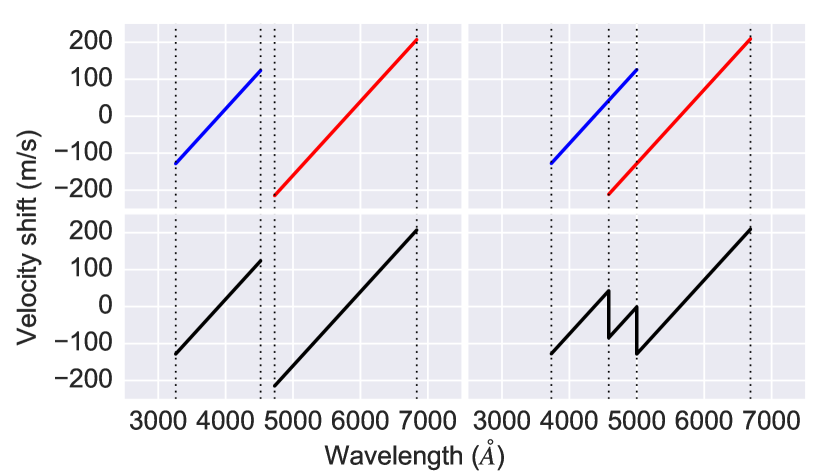
In general, each spectrum is formed by combining multiple science exposures taken at different wavelength settings. In this case the composite distortion pattern therefore depends on the central wavelength and the wavelength edges of each exposure (Fig. 1). In order to correctly estimate the actual velocity distortion at a given wavelength, one needs to take into account the details of all exposures contributing to that wavelength.

We denote $\lambda_{\mathrm{start,i}}$, $\lambda_{\mathrm{end,i}}$ be the start and end wavelength of a given science exposure of index $i$. The net velocity shift $v_{\mathrm{net}}(\lambda)$ at a given wavelength, $\lambda$, has contributions from exposures satisfying:

$$\lambda_{\mathrm{start,i}}<\lambda<\lambda_{\mathrm{end,i}}$$ (2)

The net distortion shift in the final co-added spectrum depends on the signal to noise ratio of each contributing science exposure. We therefore form the weighted net distortion function using weighting factors proportional to the square root of the exposure time for the $i^{th}$ exposure,

$$v_{\mathrm{net}}(\lambda)=\frac{\sum\limits_{i}\left(\sqrt{T_{i}}v_{\mathrm{dist,i}}(\lambda)\right)}{\sum\limits_{i}\sqrt{T_{i}}}\quad\textrm{where}\quad\lambda_{\mathrm{start,i}}<\lambda<\lambda_{\mathrm{end,i}}$$ (3)

Assuming the slope of the distortion function to be the same for every science exposures (we shall address this approximation in a separate paper), the net velocity distortion function is:

$$v_{\mathrm{net}}(\lambda)=\frac{\gamma\sum\limits_{i}\left(\sqrt{T_{i}}\left(\lambda-\lambda_{\mathrm{cent,i}}\right)\right)}{\sum\limits_{i}\sqrt{T_{i}}}$$ (4)

3 Synthetic spectra

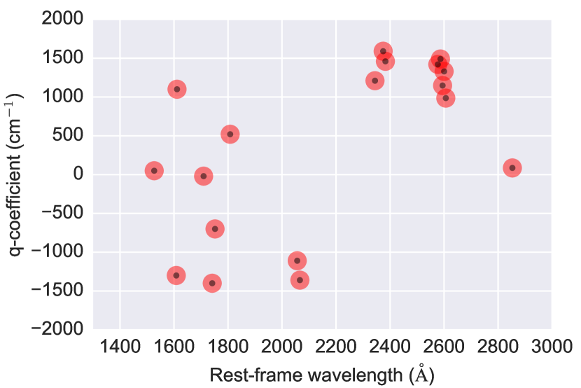
Figure 2 illustrates the $\alpha$ sensitivity coefficients, $q$, for the transitions detected in the $z_{\mathrm{abs}}=1.3554$ absorption system towards the $z_{\mathrm{em}}=1.94$ quasar J043037-485523. The overall range in $q$ is $\sim 3000$. The points are widely scattered and do not correlate tightly with rest-frame wavelength. It is this property that breaks degeneracy between the parameters $\Delta\alpha/\alpha$ and $v_{\mathrm{net}}(\lambda)$ and allows us to solve explicitly for both parameters simultaneously.

We have generated a simulated spectrum of the $z_{\mathrm{abs}}=1.3554$ absorption system towards J043037-485523, using a signal to noise per pixel of 1000, a pixel size of 2.5 km/s, and a Gaussian instrumental resolution of $\sigma=2.55$ km/s. The latter two parameters match those of actual data used previously for a measurement of $\Delta\alpha/\alpha$, (King et al., 2012).

We choose a real absorption system for this simulation to emulate reality as far as possible, albeit at very high signal to noise ratio. The useful characteristics of this system are: (1) it has a complex velocity structure, like most systems used to derive stringent constraints on $\Delta\alpha/\alpha$, (2) it exhibits a large number of transitions (20 in total), including transitions with high sensitivity to $\Delta\alpha/\alpha$, and (3) the velocity structure and other line parameters for this system are such that it yields a stringent constraint on the measurement of $\Delta\alpha/\alpha$, ($-4.05\pm 2.32$ ppm, King et al. (2012)).

Figure 2: Sensitivity to alpha against rest-wavelength for each transition used in the simulated spectrum. The q-coefficients and rest-wavelengths can be found in Table 3.

3.1 Methodology

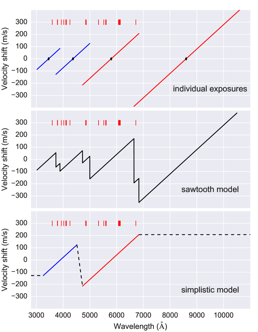
Our aim is to explore the impact on estimating $\Delta\alpha/\alpha$ using two types of distortion models to correct the spectrum. To do this we generate a simulated spectrum with known $\Delta\alpha/\alpha$ (=0) and upon which has been imposed a sawtooth distortion model of the type illustrated in the middle hand panel of Figure 3. That spectrum is then modelled in two ways: using the WM model comprising one single linear distortion function for each arm of the UVES spectrograph (illustrated in the bottom panel of Figure 3) and using the input (and more correct) sawtooth form.

The synthetic spectrum is created with random noise added, using signal to noise of 1000. We used a high S/N for these simulations to provide the accurate measurements needed to properly illustrate the importance of using a more realistic distortion model. Although S/N=1000 corresponds to an unrealistically high signal-to-noise ratio for a real quasar echelle spectrum at the present time, it may be achievable using future generations of large telescopes.

Throughout the fitting procedure, the slope of the distortion function is treated as a free parameter which we solve for simultaneously with the other “interesting” parameter, $\Delta\alpha/\alpha$, using VPFIT. In practice, the calculations were carried out in the following sequence: $\gamma=0.2\rightarrow 0.25$, then $\gamma=0.2\rightarrow 0$, in steps of $\delta\gamma=0.005$. At each successive step after the first, the starting parameter guesses supplied to VPFIT are the best-fit results from the previous step. At the two starting points, the correct (known) parameters values are used as starting guesses. The sequence and method above should make no difference to the final results (if it were done in a different sequence, we would get the same answer) but we provide the details here for completeness.

3.2 Absorption line parameters for the synthetic spectrum

The absorption line parameters used in generating the synthetic spectrum come from King et al. (2012). However, we removed the AlII 1670 and FeII 2260 transitions from the original model for the following reasons: (1) AlII 1670 was excluded because it is saturated and hence adds little in terms of sensitivity to $\Delta\alpha/\alpha$; (2) FeII 2260 was excluded because the isotopic structure is unknown (this is not the case for the other FeII transitions used in our model). Table 1 gives the line parameters used to create the synthetic spectrum. The b-parameters are taken as turbulent rather than thermal. We impose on the synthetic spectrum a sawtooth distortion model with a slope of +0.2 m/s/Å. This value is within the range of typical values measured in asteroid or solar-twin spectra. The aim is to see how well we can recover the input slope value.

Table 1: Parameter first guesses for each component fitted in the system. The first 2 columns show for each component the redshift $z$, Doppler parameter $b$ while the remaining 6 columns show the column density $N$ of each ion at each redshift location.

$z$	$b$	$\log(N_{\mathrm{MgI}})$	$\log(N_{\mathrm{SiII}})$	$\log(N_{\mathrm{CrII}})$	$\log(N_{\mathrm{MnII}})$	$\log(N_{\mathrm{NiII}})$	$\log(N_{\mathrm{FeII}})$
	[km/s]	[cm-2]	[cm-2]	[cm-2]	[cm-2]	[cm-2]	[cm-2]
1.3550877	4.6450	11.04882	13.24512	-	-	12.08916	12.86596
1.3551633	4.2369	11.01670	13.38996	-	11.17501	-	13.15444
1.3552067	4.1203	11.43565	13.52086	10.82803	11.12017	12.51781	13.13221
1.3552588	3.1190	11.16424	13.99763	12.18494	11.54568	12.52872	13.96588
1.3553108	2.0405	10.71039	13.82403	11.91851	11.43706	12.28327	13.59766
1.3553808	5.5259	11.37225	14.33999	12.39546	11.80985	12.86060	14.17853
1.3554579	1.9351	-	13.20139	-	11.04225	-	12.99883
1.3555581	7.0834	10.88266	14.28980	12.39132	11.61898	12.78850	14.01932
1.3555835	1.9147	10.41418	13.75303	11.92118	11.45834	12.03819	13.72489

3.3 Distortion model

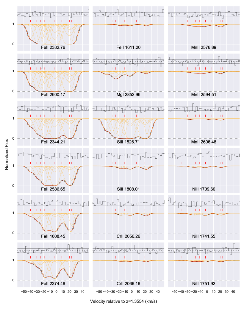
We tabulate in Table 2 all the science exposures used to produce the combined spectrum of J043037-485523. The wavelength edges of each exposure were recovered using the UVES Exposure Time Calculator . The distortion model J043037-485523 can then be built by applying Eq. 4 on the ensemble of exposures (Fig. 3). One can therefore estimate, for each transition, the value of the shift due to long-range distortion effect in the spectrum and which can be applied to the simulated spectrum to account for such distortion. Table 3 tabulates the transitions fitted, the exposures covering each region, and the velocity shift corresponding to a distortion slope of +0.2 m/s/Å. Figure 4 shows the final simulated and distorted absorption system.

Table 2: List of 18 individual science exposures for J043037-485523 in order of central wavelength combined to form the final co-added spectrum. A total of 4 different wavelength settings have been used, centered at 346, 437, 580, and 860 nm.

#	Dataset ID	$T_{\mathrm{exp}}$	arm	mode	grating	$\lambda_{\mathrm{start}}$	$\lambda_{\mathrm{cent}}$	$\lambda_{\mathrm{end}}$
		[second]				[nm]	[nm]	[nm]
1	UVES.2001-02-01T02:05:23.054	3600	BLUE	DICHR#1	CD#1	302.45	346	388.40
2	UVES.2001-03-18T00:03:50.906	3600	BLUE	DICHR#1	CD#1	302.45	346	388.40
3	UVES.2001-03-19T00:15:14.848	3600	BLUE	DICHR#1	CD#1	302.45	346	388.40
4	UVES.2001-01-13T01:28:38.684	1434	BLUE	DICHR#2	CD#2	373.24	437	499.94
5	UVES.2001-01-16T02:59:19.308	2922	BLUE	DICHR#2	CD#2	373.24	437	499.94
6	UVES.2001-02-01T03:11:26.409	3600	BLUE	DICHR#2	CD#2	373.24	437	499.94
7	UVES.2001-02-14T02:48:10.272	3600	BLUE	DICHR#2	CD#2	373.24	437	499.94
8	UVES.2001-03-05T00:19:43.715	3600	BLUE	DICHR#2	CD#2	373.24	437	499.94
9	UVES.2001-03-06T00:14:46.378	3600	BLUE	DICHR#2	CD#2	373.24	437	499.94
10	UVES.2001-02-01T02:05:21.080	3600	RED	DICHR#1	CD#3	472.69	580	683.49
11	UVES.2001-03-18T00:03:49.697	3600	RED	DICHR#1	CD#3	472.69	580	683.49
12	UVES.2001-03-19T00:15:14.827	3600	RED	DICHR#1	CD#3	472.69	580	683.49
13	UVES.2001-01-13T01:28:37.206	1437	RED	DICHR#2	CD#4	665.06	860	060.57
14	UVES.2001-01-16T02:59:21.364	2921	RED	DICHR#2	CD#4	665.06	860	060.57
15	UVES.2001-02-01T03:11:21.253	3600	RED	DICHR#2	CD#4	665.06	860	060.57
16	UVES.2001-02-14T02:48:08.997	3600	RED	DICHR#2	CD#4	665.06	860	060.57
17	UVES.2001-03-05T00:19:40.291	3600	RED	DICHR#2	CD#4	665.06	860	060.57
18	UVES.2001-03-06T00:14:41.535	3600	RED	DICHR#2	CD#4	665.06	860	060.57

Figure 3: Long-range distortion model of J043037-485523 for a distortion slope of +0.2 m/s/Å. The top panel shows the distortion pattern for each individual science exposure present in our sample. The middle panel shows the combined distortion model. The simplistic distortion model as used by WM is presented in the bottom panel, where the blue (solid line on the left) and red (solid line on the right) lines represent the long-range distortion pattern for the blue and red arms of the UVES spectrograph. The extend of the solid lines are from WM. The distortion outside the range indicated by the solid lines is assumed by WM to be constant and is represented by horizontal dashed lines. The region between both arm models are simply connected with a straight line although there seems to be no empirical justification for this. The red tick-marks on every panel illustrate the wavelength of each transition fitted in the system.

Table 3: Parameters for each fitting region in the synthetic spectrum. The first three columns specify the ion, laboratory rest-wavelength and q-coefficient for each transition. The next three columns correspond to the first, middle and last observed wavelengths for each region. The second-last column shows the range of exposures tabulated in Table 2 that covers each region of interest. Finally, the rightmost column gives the expected velocity shift at each observed central wavelength due to distortion effect when a slope of 0.2 m/s is applied to the distortion model.

Ion	$\lambda_{\mathrm{lab}}$	q	$\lambda_{\mathrm{start}}$	$\lambda_{\mathrm{cent}}$	$\lambda_{\mathrm{end}}$	Exposures	Shift
	[Å]	[cm-2]	[Å]	[Å]	[Å]	[#]	[km/s]
MgI	2852.96	86	6717.86	6719.73	6721.61	13-18	-0.1792
SiII	1526.71	50	3594.70	3595.65	3596.60	1-3	+0.0271
SiII	1808.01	520	4257.63	4258.55	4259.47	4-9	-0.0223
CrII	2056.27	-1110	4842.33	4843.25	4844.17	4-12	-0.0059
CrII	2066.16	-1360	4865.80	4866.76	4867.71	4-12	-0.0012
MnII	2576.89	1420	6068.10	6069.50	6070.90	13-18	+0.0539
MnII	2594.51	1148	6109.60	6111.05	6112.50	13-18	+0.0622
MnII	2606.48	986	6137.50	6139.00	6140.50	13-18	+0.0678
NiII	1709.60	-20	4025.50	4026.63	4027.76	4-9	-0.0687
NiII	1741.55	-1400	4100.85	4101.94	4103.04	4-9	-0.0536
NiII	1751.92	-700	4125.40	4126.50	4127.61	4-9	-0.0487
FeII	2382.76	1460	5610.96	5612.48	5614.00	10-12	-0.0375
FeII	2600.17	1330	6122.46	6124.22	6125.98	13-18	+0.0648
FeII	2344.21	1210	5520.17	5521.39	5522.60	10-12	-0.0557
FeII	2586.65	1490	6091.09	6092.53	6093.98	13-18	+0.0585
FeII	1608.45	-1300	3787.54	3788.51	3789.47	1-9	-0.0523
FeII	2374.46	1590	5591.45	5592.79	5594.13	10-12	-0.0414
FeII	1611.20	1100	3794.08	3794.93	3795.77	1-9	-0.0510

Figure 4: Velocity plot of each simulated fitting region. The VPFIT model is illustrated in red while each individual Voigt profile from each component and transition is in orange. The normalised residuals are plotted at the top of each panel.

4 Recovering $\Delta\alpha/\alpha$ and $\gamma$

In this section, we show how to recover $\Delta\alpha/\alpha$ and the distortion slope $\gamma$ from the distorted simulated spectrum. We also demonstrate that fitting the wrong distortion model can lead to significant systematic errors on both the $\Delta\alpha/\alpha$ estimates and the recovered distortion slope.

4.1 Analysis

We initially apply the distortion illustrated in the middle panel of Figure 3 to the simulated spectrum by applying fixed velocity shifts, determined from the input distortion model, to each transition. This is done directly via the VPFIT input file. The slope of the distortion model, $\gamma$, is a free parameter that we solve for.

The redshifts of corresponding velocity components in all species are tied in the fit, and since the absorption system model is turbulent, $b$-parameters of all species are also tied accordingly. This procedure is repeated for small increments of 0.005 in $\gamma$ over the range +0.1 m/s/Å to +0.25 m/s/Å. The parabolic relationship between $\chi^{2}_{\mathrm{min}}$ and $\gamma$ is fitted using a third order polynomial and the relationship between $\Delta\alpha/\alpha$ and $\gamma$ linearly, enabling us to recover the best-fit values for both parameters, with associated parameter errors.

The whole procedure above is carried out twice, once where we fit the sawtooth distortion model (i.e. the same model used to distort the simulated spectrum) to the data and again but fitting the simplistic single linear model of WM.

4.2 Results

4.2.1 Sawtooth distortion model

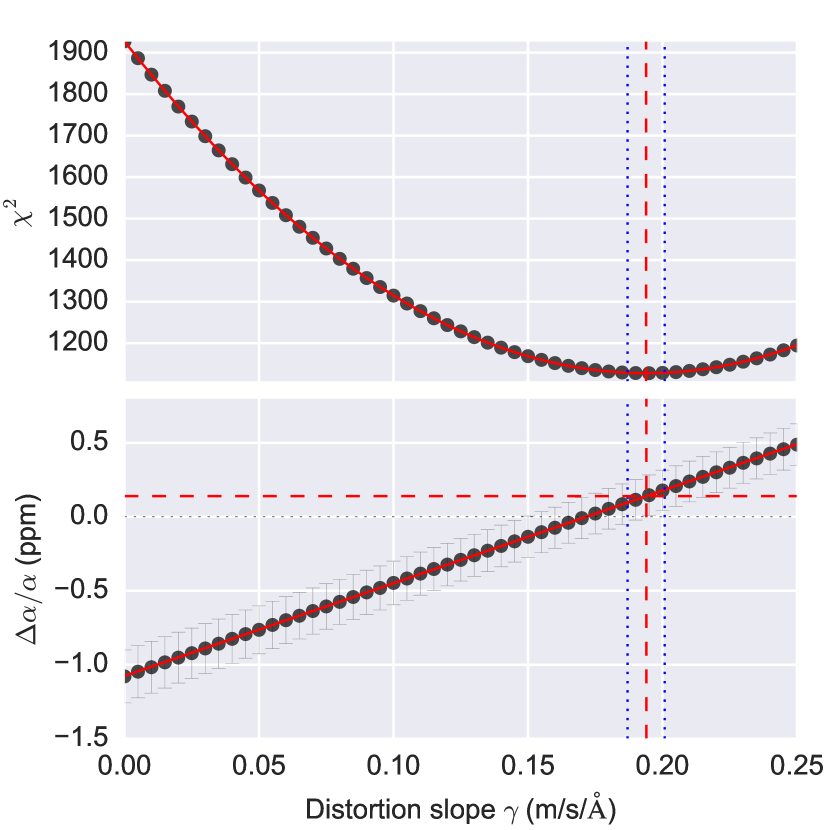
The results of fitting the simulated spectra using the sawtooth distortion model (Figure 3) are shown in Figure 5. The uncertainty on $\gamma$ is derived using the standard approach of $\chi^{2}_{\mathrm{min}}\pm 1$ for one “interesting” parameter. The uncertainty on $\Delta\alpha/\alpha$ then follows from projection of the parabolic uncertainty on $\gamma$ as Figure 5 illustrates.

Figure 5: $\chi^{2}$ and $\Delta\alpha/\alpha$ curves using the sawtooth distort ion model. The top panel shows the result from fitting the simulated spectrum using a sawtooth model, whose properties (apart from the slope, which is a free parameter) are determined by knowing the original observational details. The bottom panel shows how the inferred $\Delta\alpha/\alpha$ depends on the actual distortion slope. The best fit gives a distortion slope of $0.2062\pm 0.0073$ m/s/Å with a corresponding $\Delta\alpha/\alpha$ estimate of $-0.116\pm 0.149$ ppm.

It is worth emphasising that the uncertainties we derive are determined by the absorption system characteristics used and the high signal to noise used in these simulations. The uncertainties derived using the synthetic spectrum described above should therefore not be considered as representative of existing observational data.

After fitting the chi-square curve using a third order polynomial and the $\Delta\alpha/\alpha$ curve linearly, we find a best-fit distortion slope of $\gamma=0.2062\pm 0.0073$ m/s/Å. We thus recover the input slope of $0.2$ m/s/Å to high precision.

The recovered value of $\Delta\alpha/\alpha$ is $-0.116\pm 0.149$ ppm and is consistent with the null input value.

Over the small range in distortion slope considered, the relation between $\Delta\alpha/\alpha$ and $\gamma$ is, to a good approximation, linear. However, in general, that need not necessarily be so. As the distortion slope, $\gamma$, changes, different transitions shift by different amounts, which impacts on the measured $\chi^{2}$ for the best-fit. If we consider a large range in distortion slope, non-linearities begin to appear, and the velocity structure in the model can then even change, causing discontinuities in $\Delta\alpha/\alpha$ vs $\gamma$. We shall discuss this issue in a separate paper, although we can say here that it is generally not an important problem because $\gamma$ is usually well-constrained by the quasar spectrum itself to lie within a small range, provided there is reasonable set of transitions with a good range in q-coefficients contributing to the fit.

4.2.2 Simplistic distortion model

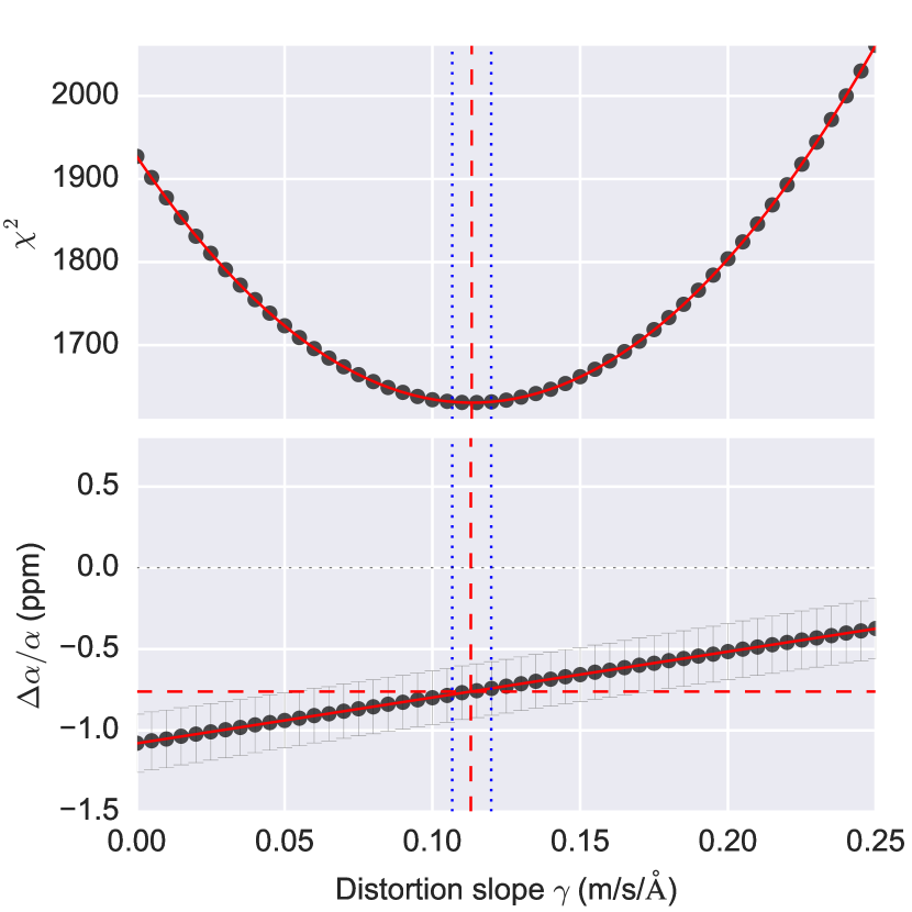
The results of fitting the simulated spectra using the simplistic linear distortion model (bottom panel of Figure 3) are shown in Figure 6. After again fitting the chi-square curve using a third order polynomial and the $\Delta\alpha/\alpha$ curve linearly, we find a best-fit distortion slope of $\gamma=0.1324\pm 0.0068$ m/s/Å, inconsistent at the 10$\sigma$ level with the correct value (i.e. the value used to create the simulated spectrum) of $0.2$.

The recovered value of $\Delta\alpha/\alpha$ is $-0.771\pm 0.173$ ppm, inconsistent with the null input value at the 4.5$\sigma$ level.

Figure 6: $\chi^{2}$ and $\Delta\alpha/\alpha$ curves using the simplistic distortion model of WM. The top panel shows the best-fit of $0.1324\pm 0.0068$ m/s/Å, 10$\sigma$ away from the true (input) value of $\gamma=0.2$. The bottom panel illustrates the “corrected” $\Delta\alpha/\alpha$ of $-0.771\pm 0.173$ ppm, a 4.5$\sigma$ departure from the true (input) value of $\Delta\alpha/\alpha$$=0$.

4.2.3 Comparison between models

It is interesting to note that a decent parabolic shape for $\chi^{2}$ vs $\gamma$ is obtained for both models. However, the inferred corrections to $\Delta\alpha/\alpha$ are quite different. The correction on $\Delta\alpha/\alpha$ inferred from the WM model shifts the result from the “uncorrected” value (corresponding to $\gamma=0$ in Figure 3) from $-1.36$ ppm to $-0.77$ ppm, i.e. a correction shift of $+0.59$ ppm. However, the corresponding shift derived from the sawtooth model is from $-1.36$ ppm to $-0.12$ ppm i.e. a correction shift of $+1.24$ ppm, more than twice as large. The latter is consistent with the true input value of zero.

We define the $\Delta\alpha/\alpha$ correction shift as the difference between the $\Delta\alpha/\alpha$ results at the best-fit distortion slope and a slope of 0. When no distortion slope is applied to the model, the resulting $\Delta\alpha/\alpha$ is found to be consistent between the two approaches, with a best-fit value of $\Delta\alpha/\alpha=-1.306\pm 0.184$.

The $\Delta\alpha/\alpha$ correction derived using the sawtooth model is more than twice as large as the $\Delta\alpha/\alpha$ correction derived using the simplistic model. The sawtooth distortion model gives a $\Delta\alpha/\alpha$ correction shift of $-0.116-(-1.306)=1.19$, the resulting shift when the simplistic distortion model is applied corresponds to $-0.771-(-1.306)=0.535$. These shifts and their uncertainties are absorption system dependent and hence need to be solved for and applied on a system-by-system basis. Whether or not these corrections translate into any kind of redshift dependence must be determined for any statistical sample.

5 Conclusions

We have investigated long-range wavelength distortions in echelle spectrographs, in the context of quasar spectroscopy, in order to quantify the impact on measurements of $\Delta\alpha/\alpha$. We created realistic numerical simulations of a known absorption system at $z_{\mathrm{abs}}=1.3554$ towards the $z_{\mathrm{em}}=1.94$ quasar J043037-485523 that has previously been used to measure $\Delta\alpha/\alpha$. Long-range wavelength distortions, based on observations of asteroids and solar-twins with the UVES instrument on the VLT, were imposed on the simulated spectra. The simulated spectra were then fitted in two ways: first using the same distortion model but treating the slope of the distortion relation as a free parameters, and second with a simplistic distortion model used previously in WM. The main results are:

• If the simplistic distortion model of WM is used to solve for long-range distortion, and hence to correct $\Delta\alpha/\alpha$ measurements, a significant systematic offset in $\Delta\alpha/\alpha$ is introduced, emulating non-zero results. The correction done in this way does not work.
  

• For the one specific absorption model we have considered, the systematic offset in $\Delta\alpha/\alpha$ introduced by using an incorrect distortion model is substantially greater than typical statistical measurement errors. This suggests that the inference of WM that long-range wavelength distortions may account for the spatial dipole reported in Webb et al. (2011) and King et al. (2012) is unlikely to be correct.
  

• If instead a more appropriate distortion model is used, allowing for the way in which almost all quasar spectra have previously been observed (using multiple wavelength settings for multiple exposures), no systematic $\Delta\alpha/\alpha$ offsets are found and the long-range distortion corrections to $\Delta\alpha/\alpha$ accurately recover the true $\Delta\alpha/\alpha$.

Clearly the quantitative results given above (i.e. the statistical significances) are model-dependent, since we simulated one particular quasar absorption system to illustrate the results. Nevertheless, the generality of the conclusions above are supported by applying the method described in this paper to the large UVES sample of $\Delta\alpha/\alpha$ measurements used in Webb et al. (2011) and King et al. (2012). That work will be reported in a separate paper.

It is not our aim in this paper to claim that the spatial dipole reported in Webb et al. (2011) and King et al. (2012) is correct. Whether that is so is still to be determined using larger statistical samples, and/or independent methods, and/or by the discovery of some systematic that explains it. However, we do wish to emphasise that no systematic effect has yet been found that emulates the spatial dipole.

References

- Griest et al. (2010) Griest K., Whitmore J. B., Wolfe A. M., Prochaska J. X., Howk J. C., Marcy G. W., 2010, ApJ , 708, 158
- King et al. (2012) King J. A., Webb J. K., Murphy M. T., Flambaum V. V., Carswell R. F., Bainbridge M. B., Wilczynska M. R., Koch F. E., 2012, MNRAS , 422, 3370
- Molaro et al. (2008) Molaro P., Levshakov S. A., Monai S., Centurión M., Bonifacio P., D’Odorico S., Monaco L., 2008, A&A , 481, 559
- Murphy et al. (2004) Murphy M. T., Flambaum V. V., Webb J. K., Dzuba V. A., Prochaska J. X., Wolfe A. M., 2004, in Karshenboim S. G., Peik E., eds, Astrophysics, Clocks and Fundamental Constants Vol. 648 of Lecture Notes in Physics, Berlin Springer Verlag, Constraining Variations in the Fine-Structure Constant, Quark Masses and the Strong Interaction. pp 131–150
- Murphy et al. (2003) Murphy M. T., Webb J. K., Flambaum V. V., 2003, MNRAS , 345, 609
- Murphy et al. (2009) Murphy M. T., Webb J. K., Flambaum V. V., 2009, Mem. Soc. Astron. Italiana , 80, 833
- Rahmani et al. (2013) Rahmani H., Wendt M., Srianand R., Noterdaeme P., Petitjean P., Molaro P., Whitmore J. B., Murphy M. T., Centurion M., Fathivavsari H., D’Odorico S., Evans T. M., Levshakov S. A., Lopez S., Martins C. J. A. P., Reimers D., Vladilo G., 2013, MNRAS , 435, 861
- Webb et al. (1999) Webb J. K., Flambaum V. V., Churchill C. W., Drinkwater M. J., Barrow J. D., 1999, Physical Review Letters, 82, 884
- Webb et al. (2011) Webb J. K., King J. A., Murphy M. T., Flambaum V. V., Carswell R. F., Bainbridge M. B., 2011, Physical Review Letters, 107, 191101
- Whitmore & Murphy (2015) Whitmore J. B., Murphy M. T., 2015, MNRAS , 447, 446
- Whitmore et al. (2010) Whitmore J. B., Murphy M. T., Griest K., 2010, ApJ , 723, 89