The Robustness of Cluster Expansion: Assessing the Roles of Relaxation and Numerical Error

Abstract

Cluster expansion (CE) is effective in modeling the stability of metallic alloys, but sometimes cluster expansions fail. Failures are often attributed to atomic relaxation in the DFT-calculated data, but there is no metric for quantifying the degree of relaxation. Additionally, numerical errors can also be responsible for slow CE convergence. We studied over one hundred different Hamiltonians and identified a heuristic, based on a normalized mean-squared displacement of atomic positions in a crystal, to determine if the effects of relaxation in CE data are too severe to build a reliable CE model. Using this heuristic, CE practitioners can determine a priori whether or not an alloy system can be reliably expanded in the cluster basis. We also examined the error distributions of the fitting data. We find no clear relationship between the type of error distribution and CE prediction ability, but there are clear correlations between CE formalism reliability, model complexity, and the number of significant terms in the model. Our results show that the size of the errors is much more important than their distribution.

I Introduction

Increasing computational power and algorithmic advancements are making many computational materials problems more tractable. For example, density functional theory (DFT) is used to assess the stability of potential metal alloys with high accuracy. However, DFT computational burdens prevent feasible exploration of all possible configurations of a system. In certain cases, one can map first-principles results on to a faster Hamiltonian, the cluster expansion (CE) Sanchez1984 ; Sanchez1993 ; Sanchez2010 . Over the past 30 years, CE has been used in combination with first-principles calculations to predict the stability of metal alloys Connolly1983 ; Ferreira1987 ; Ferreira1988 ; Ferreira1989 ; Lu1991 ; Wolverton1997 ; VandeWalle2002 ; Barabash2006 ; Asato2007 ; Nelson2013a ; Gargano2015 ; Aldegunde2016 ; Chinnappan2016 , to study the stability of oxides Ceder2000 ; Seko2006 ; Seko2008 ; Tanaka2010a ; Tanaka2010 , and to model interaction and ordering phenomena at metal surfaces Muller2003 ; Drautz2003 ; Muller2006 ; Herder2015 ; Tanaka2015 . Numerical error and relaxation effects decrease the predictive power of CE models. The aim of this paper is to demonstrate the effects of both and to provide a heuristic for knowing when a reliable CE model can be expected for a particular material system.

CE treats alloys as a purely configurational problem, i.e., a problem of decorating a fixed lattice with the alloying elements Sanchez1984 ; Sanchez1993 . However, CE models are usually constructed with data taken from “relaxed” first-principles calculations where the individual atoms assume positions that minimize the total energy, displaced from ideal lattice positions. Unfortunately, cluster expansions of systems with larger lattice relaxation converge more slowly than cluster expansions for unrelaxed systems Laks1992 . In fact, CE with increased relaxation may fail to converge altogether. No rigorous description of conditions for when the CE breakdown occurs exists in the literature.

A persistent question in the CE community regards the impact of relaxation on the accuracy of the cluster expansion. Proponents of CE argue that the CE formalism holds even when the training structures are relaxed because there is a one-to-one correspondence in configurational space between relaxed and unrelaxed structures. In this paper, we demonstrate a relationship between relaxation and loss of sparsity in the CE model. As sparsity decreases, the accuracy of CE prediction decreases.

In addition to the effects of relaxation, we also examine the impact of numerical error on the reliability of the CE fits. There are several sources of numerical error: approximations to the physics of the model, the number of $k$-points, the smearing method, basis set sizes and types, etc. Most previous studies Arnold2010 ; Diaz-Ortiz2007a ; Diaz-Ortiz2007 only examine the effect of Gaussian errors on the CE model, but Arnold et al. Arnold2010 also investigated systematic error (round-off and saturation error). They showed that, above a certain threshold, the CE model fails to recover the correct answer, that is, the CE model started to incorporate spurious terms (i.e., sparsity was reduced). A primary question that we seek to answer is how the shape of the error distribution impacts predictive performance of a CE model.

In this study, we quantify the effects of: 1) relaxation, by comparing CE fits for relaxed and unrelaxed data sets, and 2) numerical error, by adding different error distributions (i.e., Gaussian, skewed, etc.) to ideal CE models. We study more than one hundred Hamiltonians ranging from very simple pair potentials to first-principles DFT Hamiltonians. We present a heuristic for judging the quality of the CE fits. We find that a small mean-squared displacement is indicative of a good CE model. In agreement with past studies, we show that the predictive power of CE is lowered when the level of error is increased. We find that there is no clear correlation between the shape of the error profile and the CE predictive power. It is possible to decide whether the computational cost of generating CE fitting data is worthwhile by examining the degree of relaxation in a smaller set of 50–150 structures.

II Relaxation

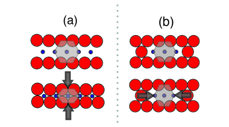
Relaxation is distinct from numerical error—it is not an error—but it has a similar negative effect. When relaxations are significant, it is less likely that a reliable CE model exists. Relaxation is a systematic form of distortion, the local adjustment of atomic positions to accommodate atoms of different sizes. Atoms “relax” away from ideal lattice sites to reduce the energy, with larger atoms taking up more room, smaller atoms giving up volume. The type of relaxations (i.e., the distortions that are possible) for a particular unit cell are limited by the symmetry of the initially undistorted case, as shown in Fig. 1. In the rectangular case (left), the unit cell aspect ratio may change without changing the initial rectangular symmetry. At the same time, the position of the blue atom is not allowed to change because doing so would destroy rectangular symmetry. In contrast, the two blue atoms in the similar structure shown in the right panel of the figure can move horizontally without reducing the symmetry.

Figure 1: (color online) Symmetry- allowed distortions for two different unit cells. The atomic positions of the cell on the left do not have any symmmetry-allowed degrees of freedom, but the aspect ratio of the unit cell is allowed to change. For the unit cell on the right, the horizontal positions of the atoms in the middle layer may change without destroying the symmetry. (The unit cell aspect ratio may also change.)

Conceptually, the cluster expansion is a technique that describes the local environment around an atom and then sums up all the “atomic energies” (environments in a unit cell) to determine a total energy for the unit cell. For the cluster expansion model to be sparse—to be a predictive model with few parameters—it relies on the premise that any specific local neighborhood contributes the same atomic energy to the total energy regardless of the crystal in which it is embedded. For example, the top row of Fig. 2 shows the same local environment (denoted by the hexagon around the central blue atom) embedded in two distinct crystals. If the contribution of this local environment to the total energy is the same in both cases, then the cluster expansion of the energy will be sparse.

The effect of relaxation on the sparsity becomes clear in the bottom row of Fig. 2. In the left-hand case [panel (a)], the crystal relaxes dramatically and the central blue atom is now four-fold coordinated entirely by red atoms. By contrast, in the right-hand case [panel (b)], a collapse of the layers is not possible and the blue atoms are allowed by symmetry to move closer to each other. From the point of view of the cluster expansion, the local environments of the central blue atom are the same for both cases. This fact, that two different relaxed local environments have identical descriptions in the cluster expansion basis, leads to a slow convergence of cluster expansion models. The problem is severe when the atomic mismatch is large and relaxations are significant (i.e., when atoms move far from the ideal lattice positions.)

Figure 2: (color online) Relaxation scheme. The top images show the original unrelaxed configurations, while the bottom figures show the relaxed configuration. The left images (a) shows the relaxation where the hexagon is contracted as shown by the black arrows in bottom left figure. The relaxation in the right images (b) is restricted to displacement of the blue atoms as shown by the black arrows in bottom right figure.

II.1 Methodology

We investigated the predictive power of cluster expansions using data from more than one hundred Hamiltonians generated from Density Functional Theory (DFT), the embedded atom method, Lennard-Jones potential and Stillinger-Weber potential. To investigate the effects of relaxation, we examined different metrics to measure the degree of atomic relaxation in a crystal configuration.

II.1.1 Hamiltonians

First-principles DFT calculations have been used to simulate metal alloys and for building cluster expansion models Ferreira1989 ; Wolverton1997 ; VandeWalle2002 ; Barabash2006 ; Asato2007 ; Nelson2013a ; Gargano2015 . However, DFT calculations are too expensive to extensively examine the relaxation in many different systems (lattice mismatch). Thus, we examine other methods such as the embedded atom method (EAM) which is a multibody potential. The EAM potential is a semi-empirical potential derived from first-principles calculations. EAM potentials of metal alloys such as Ni-Cu, Ni-Al, and Cu-Al have been parameterized from DFT calculations and validated to reproduce their experimental properties such as bulk modulus, elastic constants, lattice constants, etc. Foiles1986 . EAM potentials are computationally cheaper, allowing us to explore the effects of relaxation for large training sets; however, we are limited by the number of EAM potentials available.

Therefore, we also selected two classical potentials, Lennard-Jones (LJ) and Stillinger-Weber (SW), to adequately examine various degrees of relaxation, which can be varied using free parameters in each model. The Lennard-Jones potential is a pairwise potential. Using the LJ potential, we can model a binary ($\mathrm{A_{x}}\mathrm{B_{1-x}}$) alloy with different lattice mismatch and interaction strength between the A and B atoms by adjusting the $\sigma$ parameter in the model. Additionally, we also examined the Stillinger-Weber potential which has a pair term and an angular (three-body) term. In attempting to determine the conditions under which the CE formalism breaks down, we implemented a set of parameters in the SW potential where the angular dependent term could be turned on/off using the $\lambda$ coefficient Stillinger1985 . For example, depending on the strength of $\lambda$, the local atomic environment in 2D could switch between 3-, 4- and 6-fold coordination by changing a single parameter. Thus, when the system relaxes to a different coordination, the CE fits would no longer be valid or at least not sparse.

All first-principles calculations were performed using the Vienna Ab initio Simulation package (VASP) Kresse1993 ; Kresse1994 ; Kresse1996a ; Kresse1996 . We used the projector-augmented-wave (PAW) Blochl1994 potential and the exchange-correlation functional proposed by Perdew, Burke, and Ernzerhof (PBE) Perdew1996 . In all calculations, we used the default settings implied by the high-precision option of the code. Equivalent $k$-point meshes were used for Brillioun zone integration to reduce numerical errors Froyen1989 . We used 1728 ($12^{3}$) $k$-points for the pure element structures and an equivalent mesh for the binary alloy configurations. Each structure was allowed to fully relax (atomic, cell shape and cell volume).

Relaxation was carried out using molecular dynamics simulations for EAM, LJ and SW potentials. Two molecular dynamics packages were used to study the relaxation: GULP Gale1997 ; Gale2003 and LAMMPS Plimpton1995 . Details for the LJ, SW and EAM potentials and the DFT calculations can be found in the supplementary materials.

II.1.2 Cluster Expansion Setup

The universal cluster expansion (UNCLE) software Hart2008 ; Hart2009 ; Lerch2009 was used to generate 1000 derivative superstructures each of face-centered cubic (FCC), body-centered cubic (BCC) and hexagonal closed-packed (HCP) lattice. For the DFT calculations, we used only 500 structures instead of 1000 due to the computational cost. We generated a set of 1100 clusters, ranging from 2-body up to 6-body interactions. 100 independent CE fits were performed for each system (Hamiltonian and lattice).

We performed cluster expansions using the UNCLE software Lerch2009 . We briefly discuss some important details about cluster expansion here, but for a more complete description, see the supplementary materials and past works Connolly1983 ; Sanchez1984 ; Ferreira1991 ; Zunger2002 ; VandeWalle2002 ; VandeWalle2013 ; Nelson2013 ; Nelson2013a . Cluster expansion is a generalized Ising model with many-body interactions. The cluster expansion formalism allows one to map a physical property, such as E, to configuration ($\overrightarrow{\sigma}$):

$$E_{i}^{\mathrm{CE}}=\Sigma_{i}J_{i}\Pi_{i}(\overrightarrow{\sigma})$$ (1)

where E is energy, $\Pi$ is the correlation matrix (basis), and $J$ is coefficient or effective cluster interaction (ECI).

When constructing a CE model, we are solving for the effective cluster interactions, or $J$s. We used the compressive sensing (CS) framework to solve for these coefficients Nelson2013 ; Nelson2013a . The key assumption in compressive sensing is that the solution vector has few nonzero components, i.e., the solution is sparse Candes2006 ; Candes2008 . The CS framework guarantees that the sparse solution can be recovered from a limited number of DFT energies. Using the $J$s, we can build a CE model to interpolate the configuration space.

Each CE fit used a random selection of 25% of the data for training and 75% for validation. Results were averaged over the 100 CE fits with error bars computed from the standard deviation. We defined the percent error as a ratio of the prediction root mean squared error (RMS) over the standard deviation of the input energies, $\mathrm{percent\ error}=\mathrm{RMS}/\mathrm{STD(E_{input})}\times 100\%.$ This definition of percent error allowed us to consistently compare different systems.

II.1.3 Relaxation Metrics

Currently, there is no standard measure to indicate the degree of relaxation. We evaluated different metrics as a measure of the relaxation: normalized mean- squared displacement, Ackland’s order parameter Ackland2006 , difference in Steinhardt order parameter ($D_{6}$) Steinhardt1983 , SOAP Bartok2013 , and the centro-symmetry parameter Kelchner1998 . We compared the metrics across various Hamiltonians to find a criterion that is independent of the potentials and systems . We found that none of these metrics are descriptive/general enough except for the normalized mean- squared displacement.

II.1.4 Normalized Mean-Squared Displacement (NMSD)

To measure the relaxation of each structure/configuration, we used the mean- squared displacement (MSD) to measure the displacement of an atom from its reference position, i.e., the unrelaxed atomic position. The MSD metric is implemented in the LAMMPS software Plimpton1995 , which also incorporates the periodic boundary conditions to properly account for displacement across a boundary. The MSD is the total squared displacement averaged over all atoms in the crystal:

$$\mathrm{MSD}=\frac{1}{N_{\mathrm{atom}}}\sum_{\mathrm{atom}}\sum_{X=x,y,z}(X[t]-X[0])^{2}$$ (2)

where $t$ is the final relaxed configuration and 0 is the initial unrelaxed configuration. Additionally, we defined a normalized mean-square displacement (NMSD) percent:

$$\mathrm{NMSD}=\frac{\mathrm{MSD}}{V^{2/3}}\times 100\%$$ (3)

which is the ratio of MSD to volume of the system. This allows for a relaxation comparison parameter that is independent of the overall scale.

II.2 Results and Discussions

To explore the effects of relaxation on CE predictability, we examine relaxation in various systems from very high accuracy (DFT) to very simple, tunable systems (LJ and SW potentials). We examine more than one hundred different Hamiltonians and we find several common trends among the different systems.

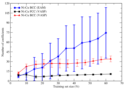
In most cases, we find that the relaxed CE fits are worse (higher prediction error and higher number of coefficients) than the unrelaxed. For example, Fig. 3 shows the cluster expansion fitting for unrelaxed and relaxed data sets of Ni-Cu alloy system using DFT and EAM with two different primitive lattices. Though it seems strange for us to model Ni- Cu using a BCC primitive lattice when Ni-Cu is closed-packed, this is a method for us to evaluate the relaxation of Ni-Cu for a highly relaxed system. As Fig. 3 shows, Ni-Cu alloy fitting for a FCC lattice is below 10% error, while BCC fitting result in more $J$s and higher percent error (above 10%) . We find similar results in the relaxation of Ni-Cu alloy using first-principles DFT and EAM potential. The difference between relaxed and unrelaxed CE fits are negligible when relaxations are small. This is shown in fig. 3 for the relaxation of FCC superstructures using a Ni-Cu EAM potential.

Figure 3: (color online) Cluster expansion fits for Ni-Cu alloy using DFT or EAM potential. Each bar represents the average percent error and error bar (standard deviations) for 100 independent CE fits. The blue bars represent the unrelaxed CE fits, while the red bars represent the relaxed CE fits. The colored number represents the average number of coefficients used in the CE models. When the configurations are relaxed, we find that the CE fits are often worse (higher prediction error and higher number of $J$s) than unrelaxed system. However, we show that in one case (Ni-Cu EAM) the unrelaxed and relaxed CE fits are identical (same error and same number of coefficients) and this is due to a small relaxation.

(a) Histogram of clusters in 4(b)

(b) CE fits vs clusters for FCC parent lattice

(c) CE fits vs $J$s

(d) CE fits vs errors

(e) Histogram of clusters in 4(f)

(f) CE fits vs clusters for BCC derivative structures

(g) CE fits vs $J$s

(h) CE fits vs errors

Figure 4: (color online) CE fitting and relaxation of Ni-Cu alloys using FCC derivative superstructures and BCC derviative superstructures. Shown in Fig. 4(b) and 4(a) are the 100 CE fits and the histogram of the clusters used for the FCC lattices, while plot 4(f) and 4(e) are for the BCC lattice. The errors and coefficients are shown in 4(c) and 4(d) for the FCC structures, and in 4(g) and 4(h) for the BCC lattice. The plot shows that the number of clusters used in fitting is small when cluster expansion fitting is good (error is on average 6.03% for FCC derivative structures). However, the CE fitting of BCC parent lattice is worse at 16.70% compared to FCC at 6.03%. More coefficients are used when CE fails. The increased number of $J$s and error indicate a bad CE fitting model as shown by plots 4(g) and 4(h). Fig. 4(e) shows only a few significant terms with many other clusters used sparingly in the fits.

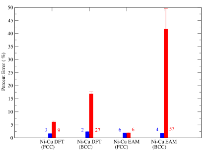
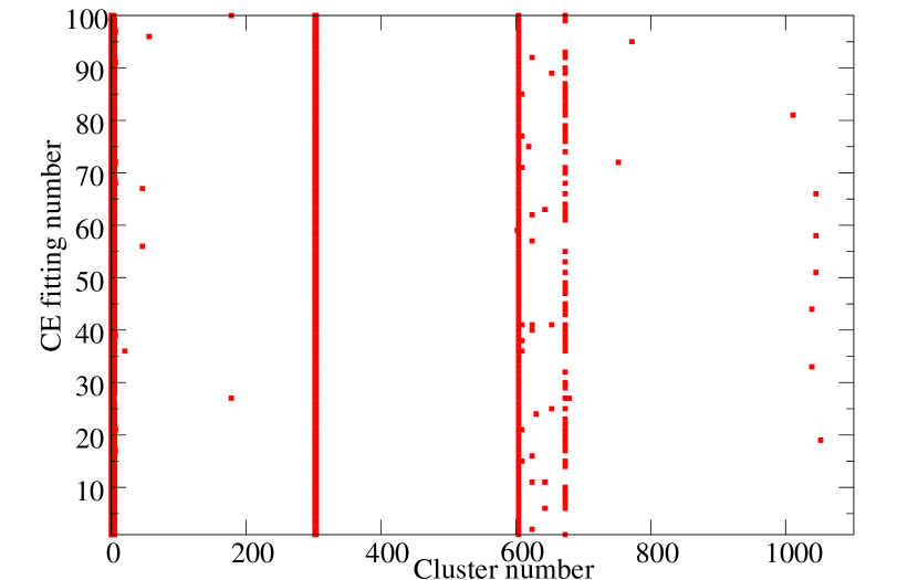
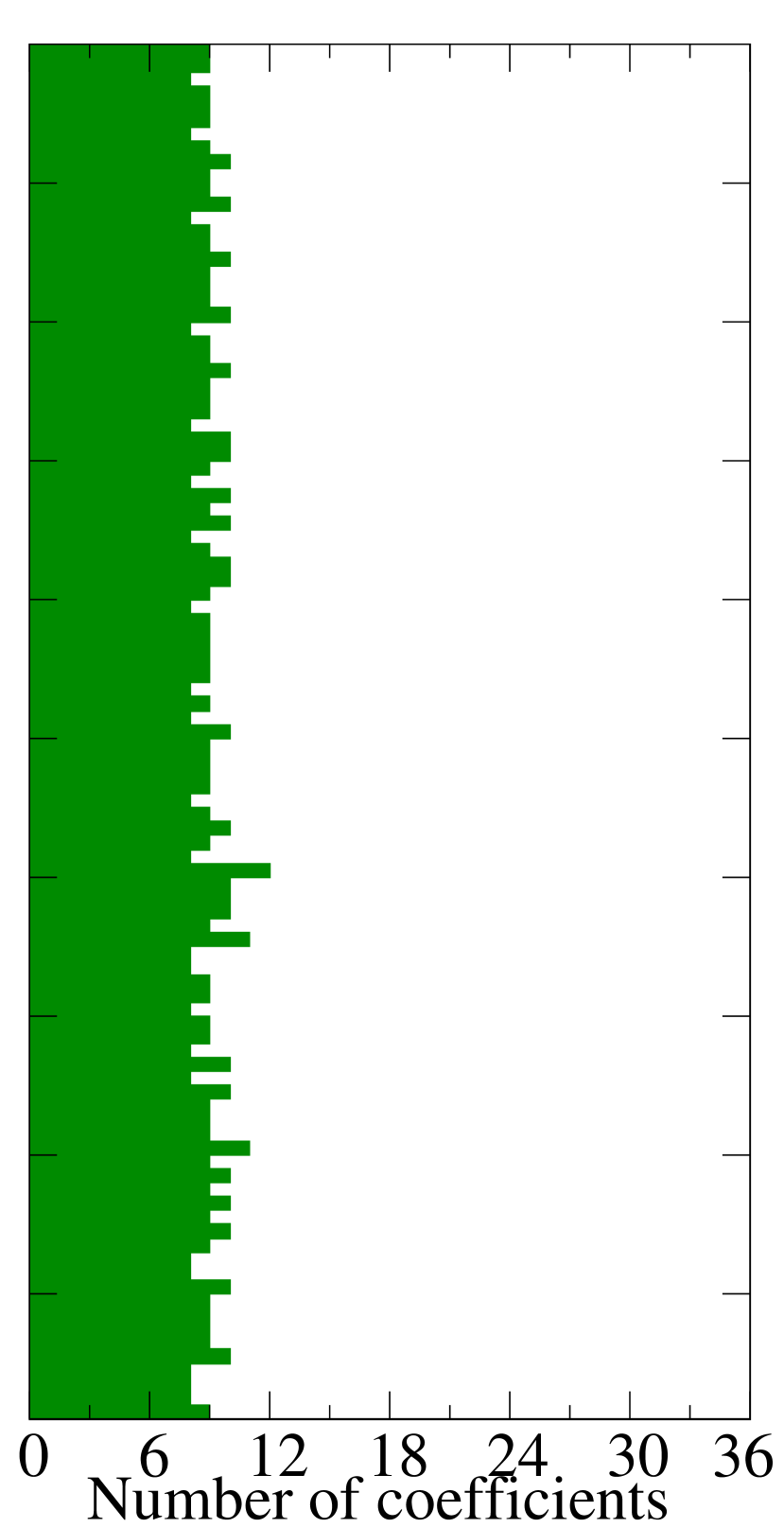
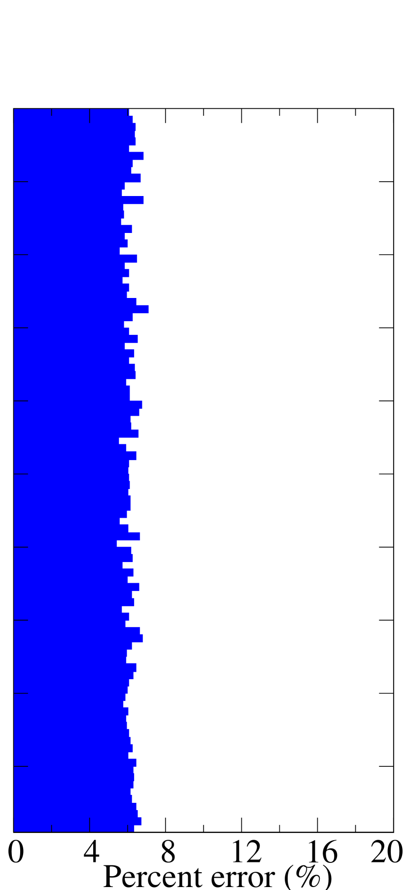
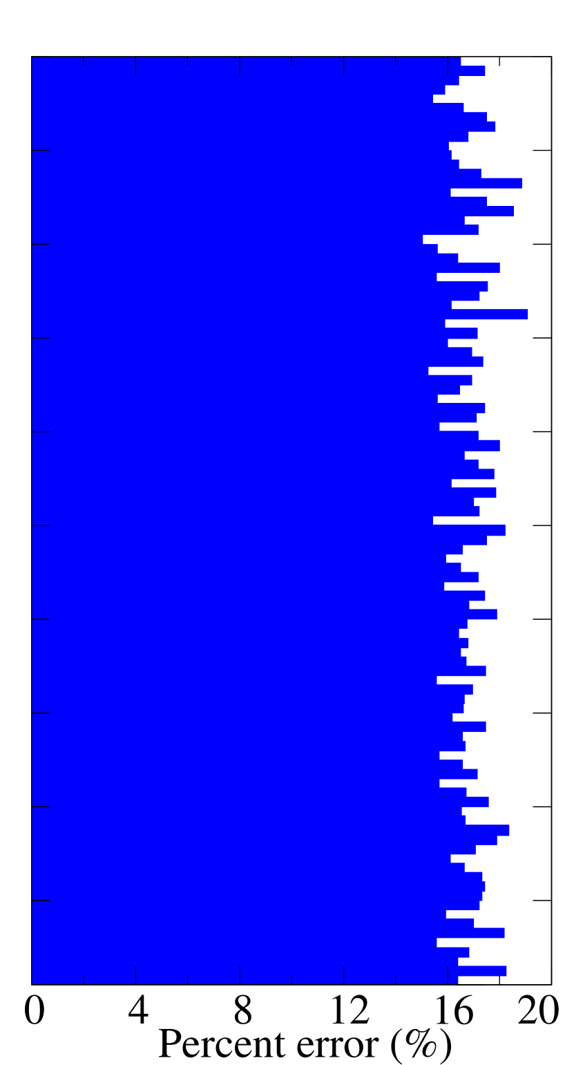
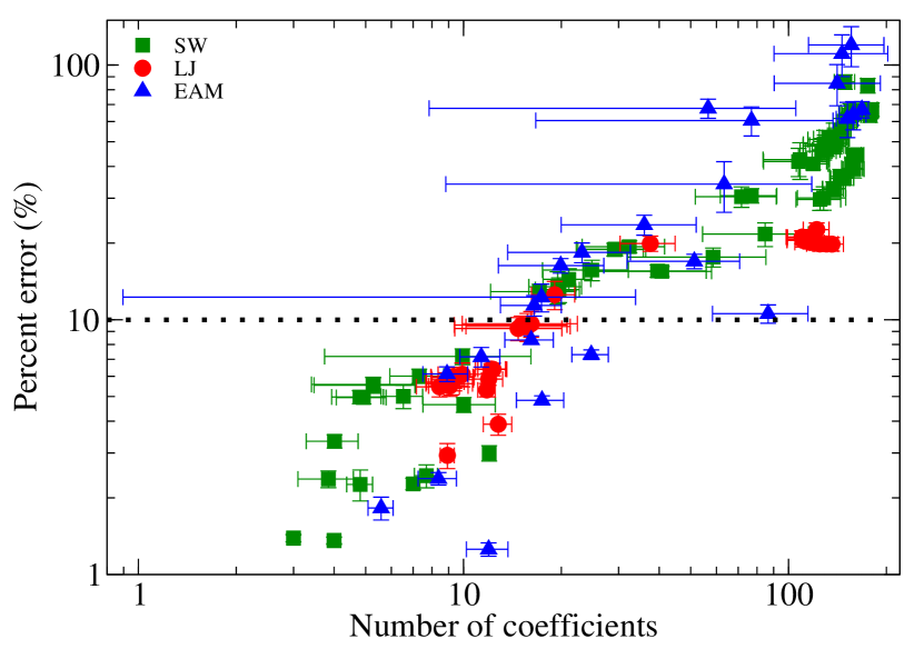
Fig. 3 shows that increased relaxation is associated with reduced sparsity (increased cardinality of $J$s). One possible implication is that number of coefficients ($J$) could be used to evaluate the predictive performance of the CE fits. The number of coefficients used in the fits (such as in fig. 3) is a simple way to determine whether or not a CE fit can be trusted. Fig. 4(b) and 4(f) show similar clusters across the 100 independent CE fittings; thus, vertical lines indicate the presence of the same cluster across all CE fits. When the fit is good, only a small subset of clusters is needed (Fig. 4(b)). On the other hand, Fig. 4(f) shows some common clusters in all of the CE fits with several additional clusters. Fig. 5(a) shows the correlation of the percent error with the number of terms in the expansion. We find that as the number of coefficients increases the percent error increases. However, this is not a sufficient metric as shown in Fig. 5(a) where the number of coefficient varies a lot. Nonetheless, the number of coefficients may be used as a general, quick test.

(a) Error vs $J$s

(b) Relaxation vs $J$s

Figure 5: (color online) Plot 5(a) displays the CE fitting error vs the number of coefficients, while plot 5(b) highlights the relationship between number of coefficients and relaxation. The dashed line approximates what we consider as the maximum acceptable error for a CE model (10%). The dashed line in Fig. 5(b) marks the estimated threshold for acceptable relaxation level. Each symbol represents 100 independent CE fittings for each Hamiltonian. Higher error correlates with a higher number of coefficients.

The degree of relaxation is crucial to define whether or not the CE model is accurate or not. However, there is no standard for when cluster expansion fails due to relaxation. Thus far, we have made some remarks about relaxation and CE fits. But the question of how much relaxation is allowed has not been addressed. By examining a few metrics: NMSD, SOAP Bartok2013 , D6 Steinhardt1983 ,Ackland Ackland2006 and centro-symmetry Kelchner1998 , we find that there is a relationship between degree of relaxation and the quality of CE fits. As shown in the supplementary information, we have used these metrics to investigate over 100+ systems (different potentials, lattice mismatches, and interaction strengths). Here, we present a heuristic to measure the degree of relaxation based on the NMSD.

In general, cluster expansion will fail when the relaxation is large. Figure 5(b) shows that a small NMSD weakly correlates with a small number of coefficients. However, Figure 6 highlights the correlation between degree of relaxation and prediction error. There is a roughly linear relationship between the degree of relaxation and the CE prediction. We partition the quality of the CE models into three regions: good (NMSD $<$ 0.1%), maybe (0.1% $\leq$ NMSD $\leq$ 1%) and bad (NMSD $>$ 1%). The “maybe” region is the gray area where the CE fit can be good or bad. This metric provide a heuristic to evaluate the reliability of the CE models, i.e., any systems that exhibit high relaxation will fail to provide an accurate CE model.

Figure 6: (color online) Relationships between relaxation and CE fitting reveal a heuristic for determining the quality of a CE model. This graph shows the CE fitting error vs normalized mean square displacement (NMSD). Each mark represents 100 individual CE fittings for each system (potentials and parameters). As the NMSD (relaxation) increases, the CE fitting error increases for various systems and potentials. Using the relaxation metric, the quality/ reliability of the CE fits can be divided into three regions: good, maybe and bad CE model. The solid black lines indicates these three areas.

III Numerical Error

As we have shown in the previous section, greater relaxation results in worse CE fitting. In addition to the effects of relaxation, we now investigate the effects of numerical error on reliability of CE models. Numerical error arises from various sources such as the number of $k$-points, the smearing method, minimum force tolerance, basis set sizes and types, etc. These errors are not stochastic error or measurement errors; they arise from tuning the numerical methods. We assume that the relaxation-induced change in energy for each structure is an error term that the CE fitting algorithm must handle. The collection of these “errors” from all structures in the alloy system then form an error profile (or distribution). Using the simulated relaxation error profiles from the previous section together with common analytic distributions, we built “toy” CE models with known coefficients. We then examined whether or not the shape of the error distribution affects the CE predictive ability.

III.1 Methodology

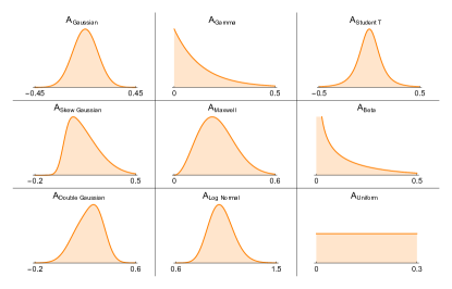
The numerical errors in DFT calculations are largely understood, but it is difficult to disentangle the effects of different, individual error sources. Instead of studying the effects of errors separately, we added different distributions of error to a “toy” model in order to imitate the aggregate effects of the numerical error on CE models. Hence, we opt to simplify the problem by creating a “toy” problem for which the exact answer is known. To restrict the number of independent variables, we formulated a “toy” cluster expansion model by selecting five non-zero values for a subset of the total clusters. Using this toy CE, we predicted a set of energies $y$ for 2000 known derivative superstructures of an FCC lattice, These $y$ values are used as the true energies for all subsequent analysis. We added error to $y$, chosen from either: 1) “simulated” distributions obtained by computing the difference between relaxed and unrelaxed energies predicted by either DFT, EAM, LJ or SW models (Fig. 7); or 2) common analytic distributions (Fig. 8).

To generate the simulated distributions, we chose a set of identical structures and fitted them using a variety of classical and semi-classical potentials, and quantum mechanical calculations using VASP. For each of the potentials we selected, we calculated an unrelaxed total energy $y$ for each structure and then performed relaxation to determine the lowest energy state, $\tilde{y}$. The difference between these two energies ($\Delta y=\tilde{y}-y$) was considered to be the “relaxation” error.

Figure 7: (color online) Distributions from real relaxations using classical and semi-classical potentials, as well as DFT calculations. The distributions are all normalized to fall within 0 and 1. The widths, $\Delta$, were calculated by taking the difference between the 25${}^{\textrm{th}}$ and 75${}^{\textrm{th}}$ percentiles.

Figure 8: (color online) The analytic, equal width distributions used for adding error to the toy model CE fit.

Certain assumptions are usually made about the error in the signal, namely that it is Gaussian. The original CS paradigm proves that the $\ell_{2}$ error for signal recovery obeys Candes2008 :

$$\left|\left|x^{*}-x\right|\right|_{\ell_{2}}\leq C_{0}\cdot\left|\left|x-x_{S}\right|\right|/\sqrt{S}+C_{1}\cdot\epsilon,$$ (4)

where $\epsilon$ bounds the amount of error in the data, $x^{*}$ is the CS solution, $x$ is the true solution, and $x_{S}$ is the vector $x$ with all but the largest $S$ components set to zero. This shows that, at worst, the error in the recovery is bounded by a term proportional to the error. For our plots of this error, we first normalized $\Delta{y}$ so that $\epsilon\equiv\mathrm{normalized}(\Delta y)\in[0,1]$ using

$$\epsilon=\frac{y-\mathrm{min}(y)}{\mathrm{max(y)}-\mathrm{min}(y)}.$$ (5)

Not surprisingly, the various potentials produced different error profiles.

The expectation value of the distributions was set to be a percentage of the average, unrelaxed energy across all structures. Thus, “15% error” means that each unrelaxed energy was changed by adding a randomly drawn value from a distribution with an expectation value of 15% of the mean energy. We performed CE fits as a function of the %-error added (2,5,10 and 15%) for each distribution. Although we only present the 15% error results in the next section, all results at different error levels can be found in the supporting information. For each data point, we performed 100 independent CE fits and used the mean and standard deviation to produce the values and error bars for the plots.

III.2 Results and Discussions

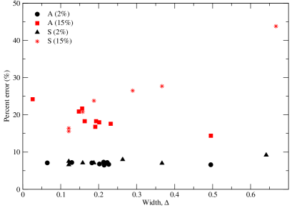
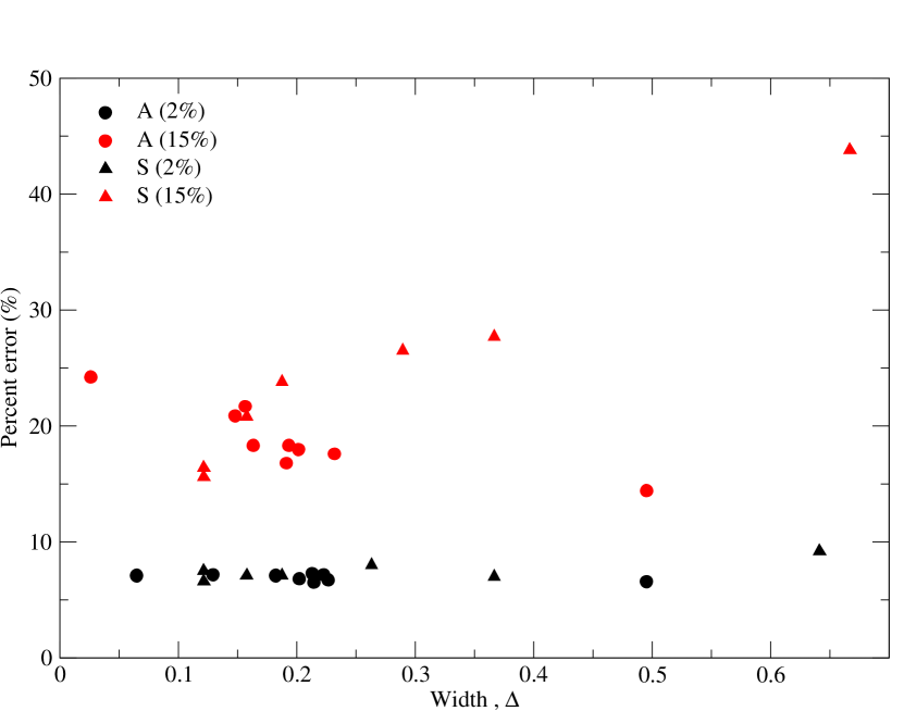
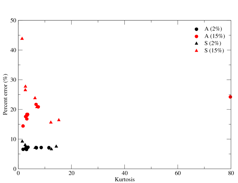
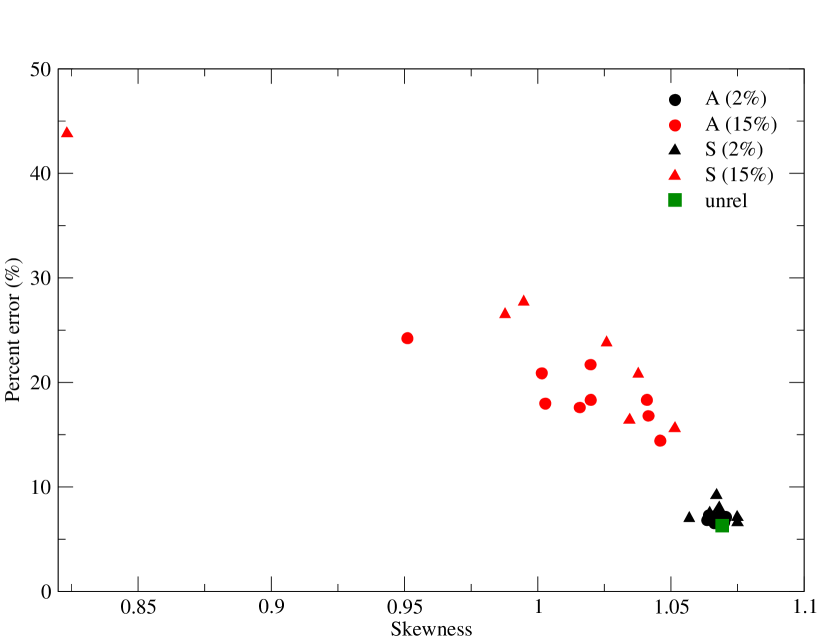
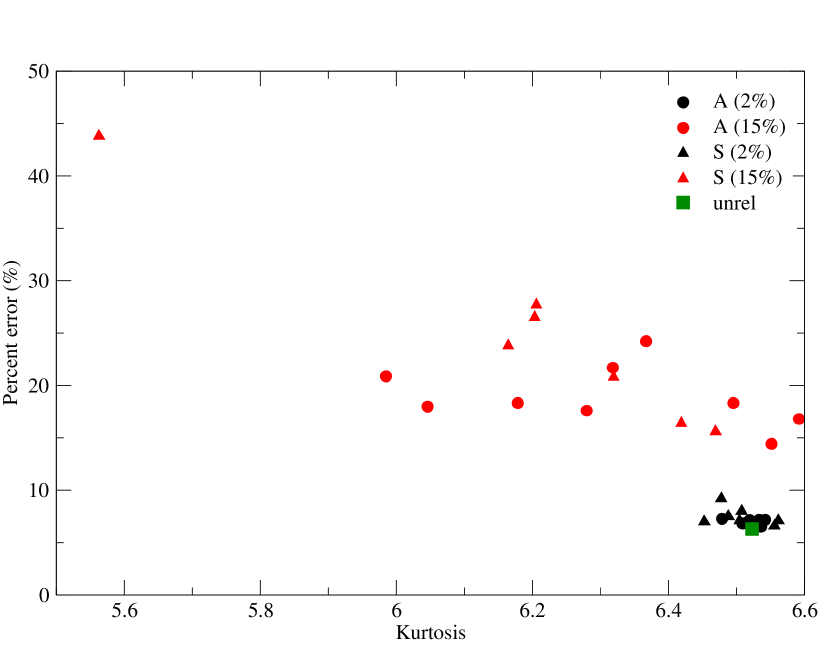
As shown in Fig. S6, the error is weakly uniform across all (analytic and simulated) distributions, implying that there is no correlation between specific distribution and error. None of the normal quantifying descriptions of distribution shape (e.g. width, skewness, kurtosis, standard deviation, etc.) show a correlation with the CE prediction error. The error increased proportionally with the level of error in each system (2, 5, 10 and 15% error). We therefore turn to the compressive sensing (CS) formalism for insight.

Figure 9: (color online) Comparison of the predictive error in CE fits as the shape of relaxation error changes. (A) refers to the analytic distribution while (S) refers to simulated distribution. The fits are ordered from lowest to highest distribution width. Fits were averaged over 100 randomly selected subsets with 500/2000 data points used for training; the remaining 1500 were used to verify the model’s predictions. The black and red colored symbols represent 2% and 15% error levels, respectively. The circles and triangles represent the analytical and simulated distributions, respectively. Higher error produces higher prediction errors.

The theorems of Tao and Candés Candes2006 guarantee that the solution for an underdetermined CS problem can be recovered exactly with overwhelming probability provided:

• The solution is sparse within the chosen representation basis.

• Sufficient data points, sampled independent and identically distributed (i.i.d).

• The sensing and representation bases are maximally incoherent.

If all of these conditions are met, we know that CS will provide a solution that is very close to the true answer. Conversely, if CS cannot converge to a good solution, it means that one of these conditions has been violated. We have control over the number of training points, and the incoherence of the sensing- representation bases. However, we cannot control whether the true physical solution is sparsely represented for relaxed systems. This suggests a useful connection between the CS framework and the robustness of CE: if CS cannot reproduce a good CE fit (quantified below), then sparsity has been lost.

In the CS framework, the foundational assumption is that of sparsity, meaning that the compressed signal (or cluster expansion) requires only a few terms to accurately represent the true signal (physics). Thus, the number of terms recovered by CS to produce the CE is a good measure of the quality of the CS fit. This begs the question: can we use the number of terms within the CS framework to heuristically predict in advance whether the CE fit will converge well?

In answering the question of predictability for a good CE fit, we define three new quantities:

1. $\Xi$: total number of unique clusters used over 100 CE fits of the same dataset. We also call this the model complexity.

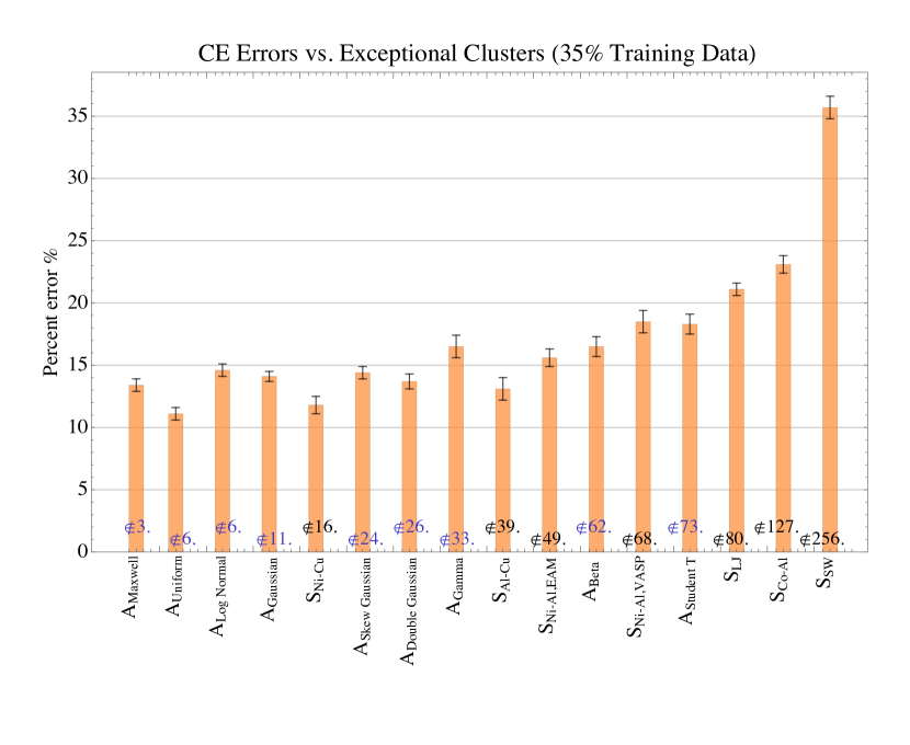
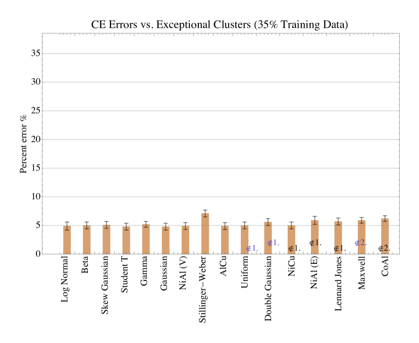
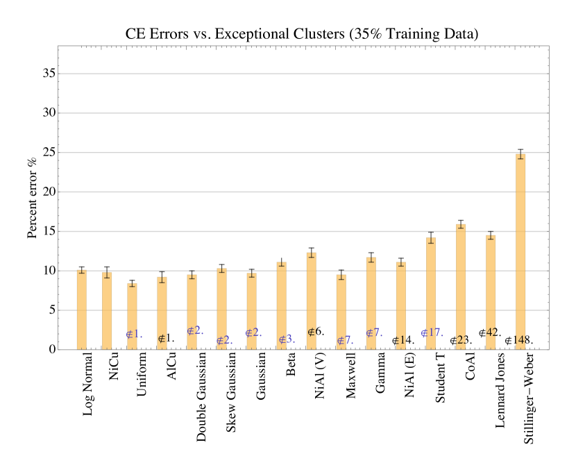
2. $\not\in$: number of “exceptional” clusters. These are clusters that show up fewer than 25 times across 100 fits, implying that they are not responsible for representing any real physics in the signal, but are rather included because the CE basis is no longer a sparse representation for the relaxed alloy system. They are sensitive to the training/fitting structures.

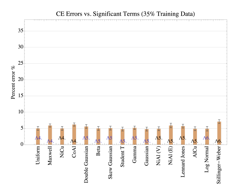
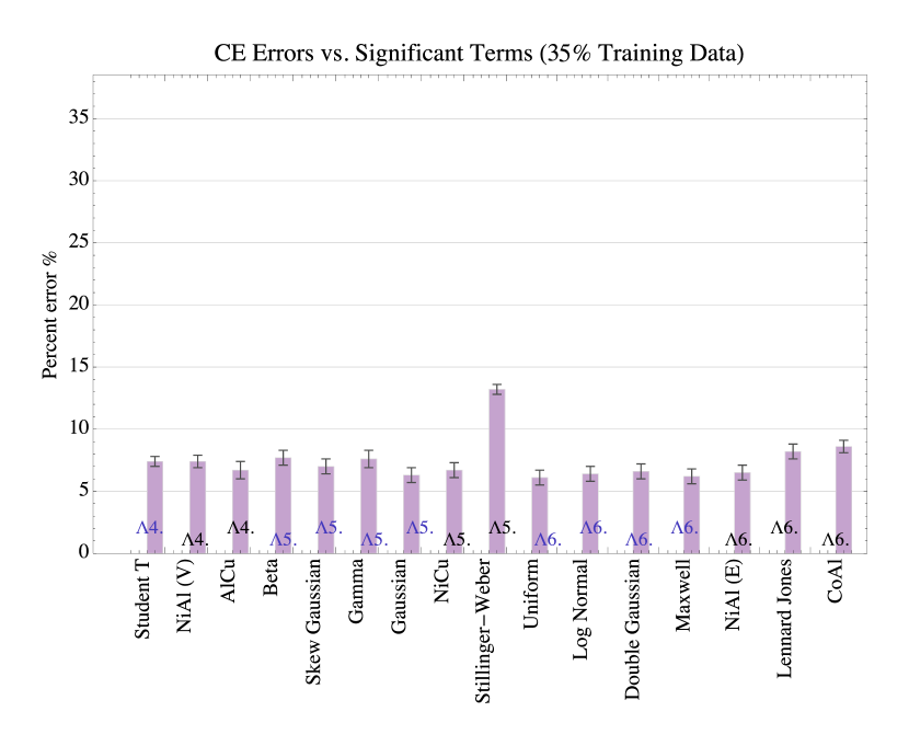
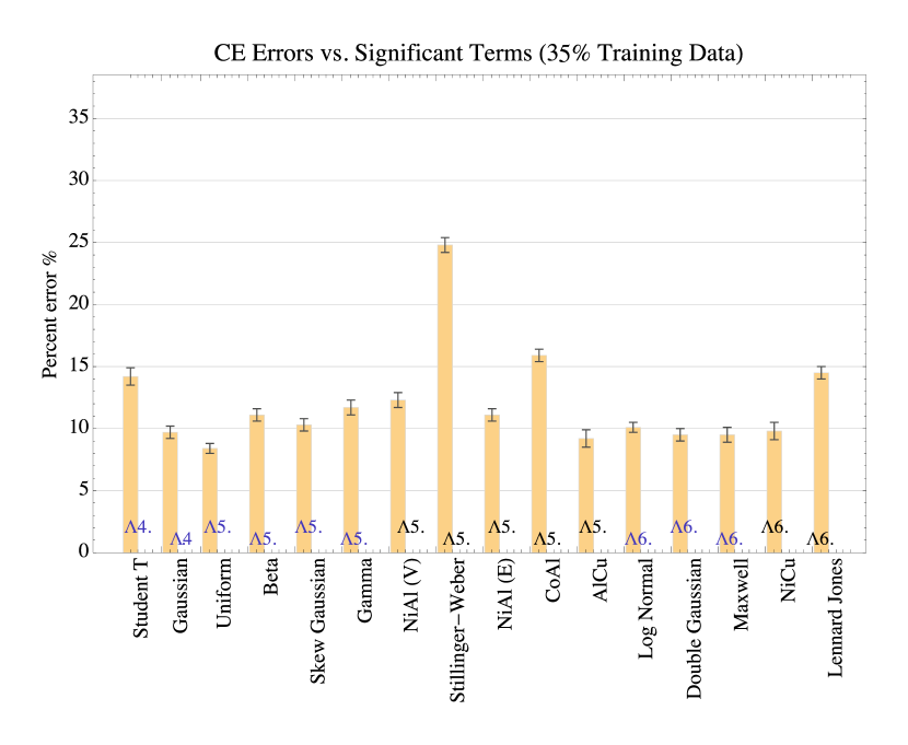
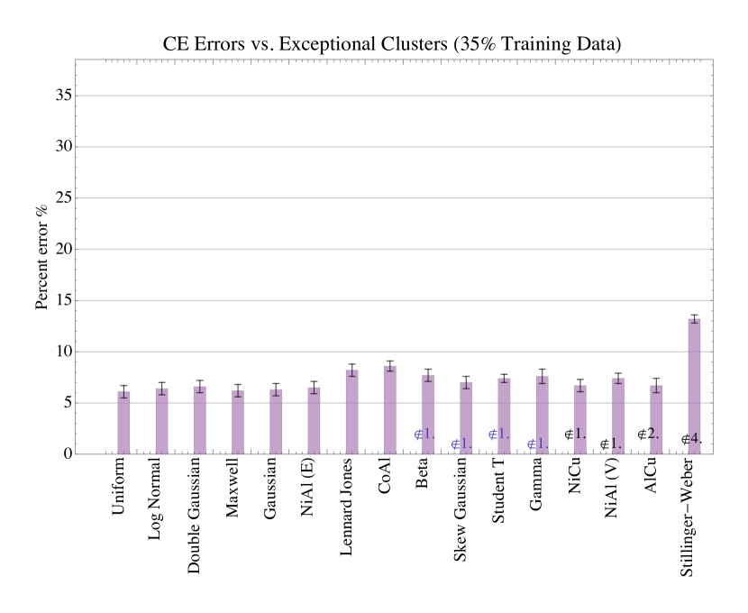
3. $\Lambda$: number of significant clusters in the fit; essentially just the total number of unique clusters minus the number of “exceptional” clusters, $\Lambda=\Xi-\not\in$.

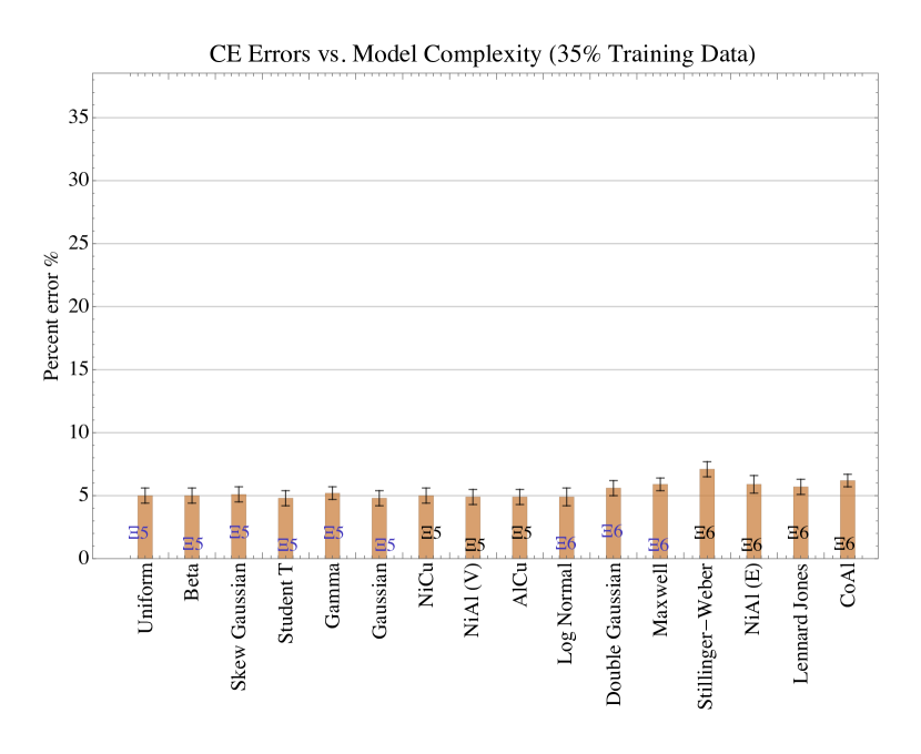
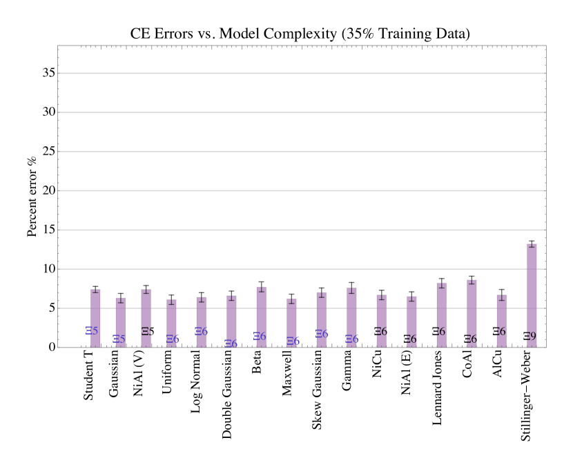
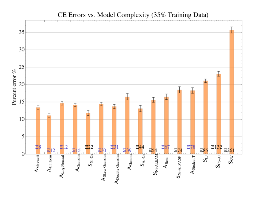
In the relaxation section, we showed that the average number of coefficient is not sufficient to determine the quality of the CE model. Here, we decompose the number of $J$s into three new quantities to provide additional insights into the reliability of the CE fits. In Fig. S8, we plot the CE error, ordered by model complexity and show that it reproduces the trend identified by the number of coefficients (indeed they are intimately related, $\Xi$ being the statistically averaged number of coefficients across many fits). An ordering by the number of exceptional clusters $\not\in$ produces an identical trend, showing that it may also serve to quantify a good fit .

Figure 10: (color online) Prediction error over 65% of the structures for the “toy” cluster expansion (at 15% error added). The systems are ordered by $\Xi$, which is the total number of unique clusters used by any of the 100 CE fits for the system. This ordering shows a definite trend with increasing $\Xi$.

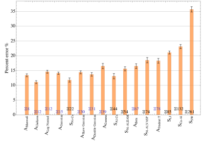
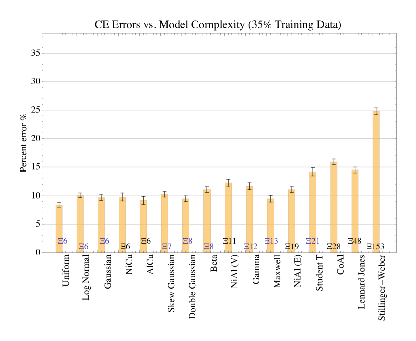
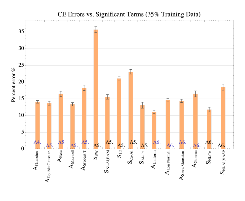
As indicated earlier, all these experiments were performed for a known CE model that had 5 non-zero terms. Additional insight is gained by plotting the errors, ordered by $\Lambda$, the number of significant clusters (Fig. S10). Fig. S10 shows that in almost all cases, once we remove the exceptional clusters $\not\in$, the remaining model is almost exactly the known CE model that we started with. The CS framework provides a rigorous mathematical framework for this statement because it guarantees to exactly recover the original function with high probability as long as we have enough measurements and our representation basis is truly sparse. Once the cluster expansion stops converging, we lose sparsity and CS fails. This gives us confidence to use the CS framework as a predictive tool for CE robustness.

Figure 11: (color online) Prediction error over 65% of the structures for the “toy” CE model (at 15% error added). The errors are ordered by $\Lambda$, the number of significant terms in the expansion. As expected, the values are close to the known model complexity (5 terms) and the ordering once more appears random.

Provided the training structures are independent and identically distributed, we do not necessarily need hundreds of costly DFT calculations to tell us that the CE will not converge. Using our toy CE model, we discovered that for all error distributions, a training set size of 50 data points was sufficient to recover the actual model complexity (5 terms) . For actual DFT calculations, where relaxation was known to disrupt CE convergence, we saw a similar trend with about 100 data points needed to identify whether the CE would converge with more data or not.

We conclude that CE robustness for relaxed systems can be predicted with a much smaller number of data points than is typically needed for a good CE fit (on the order of 5-10% from our experience) . The proposed heuristic to verify convergence of the relaxed CE, when trained with a limited dataset, is to examine the values of $\Lambda$ and $\Xi$ over a large number of independent fits. If the number of the exceptional clusters $\not\in$ is significant compared to $\Lambda$, then it is likely that the CE will not converge on a larger dataset as shown in Fig. S9. Figure 13 highlights the CE fitting as function of training set size. We observe small relaxation (black curve) correlates with a small number of coefficients; thus the CE can fit using a small number of $J$s even with 5% (25) to 10% (50) of the structures. On the other hand, red and blue curves which have high relaxation, do not converge. By using a small relaxed dataset (50 to 100 structures), we can predict whether or not the computational cost of relaxing many structures is fruitful.

Figure 12: (color online) Plot of predictive error over 65% of the structures for the “toy” problem (at 15% error added). The systems are ordered by $\not\in$ the number of clusters that were used less than 25 times across all 100 CE fits. These are considered exceptions to the overall fit for the system. As for Figure S8, there is a definite trend toward higher error for systems with more exceptional clusters.

Figure 13: (color online) For a reliable CE model, the number of coefficients converges as a function of the training set size. A total of 500 structure were available for training. The number of coefficients in a fit and its error bars give us an indication of the predictive power of CE with only a small training set. The black curve represents a good CE fit; only 25 to 50 (or 5 to 10%) of training structures were needed. On the other hand, the red and blue curves show that CE fails to fit the data due to a slowly converging expansion. The error bars on the blue points indicate extremely bad fitting.

IV Conclusions

Relaxation and error decrease the reliability of the cluster expansion fit because the CE model is no longer sparse. Nevertheless, until now, there has been no measure of relaxation that provides a heuristic as to when the CE fitting data is reliable. Using four different Hamiltonians (first-principles, Lennard-Jones, Stillinger-Weber and embedded atom method), we show that the normalized mean-squared displacement of alloy configuration is a good measure of relaxation and CE predictability. A small displacement percent, e.g., less than 0.1%, will usually generate a reliable CE model. The number of cluster terms in the CE models is also a good indicator of how well cluster expansions can perform. As the number of clusters increases, the predictability of CE model decreases. CE tends to fail when the number of $J$s exceeds 80.

In our error analysis, we investigated the ability of the compressive sensing framework to obtain fits to a toy, cluster expansion model as the energy of relaxation changes in a predictable way. We used 16 relaxation error distributions (both analytic and simulated) and compared the prediction errors of the resulting CE fits for the relaxed vs. unrelaxed case. No clear correlation appears between the statistical measures of distribution shape and the predictive errors. However, there are clear correlations between the predictive error, the complexity of the resulting CE model, and the number of significant terms in that model.

We cannot use the relaxation distributions alone to determine the viability of a CE fit in advance. However, the analysis does reveal that the majority of the clusters used by the unrelaxed CE fit will also be present in the relaxed case (albeit with adjusted $J$ values) if the CE fit is viable. This suggests that it may be possible to decide whether the computational cost of full CE is worthwhile by making predictions for a few relaxed systems (50-100) and determining whether the error remains small enough.

V Acknowledgments

The authors thank Volker Blum, Lance J. Nelson and Mark K. Transtrum for useful discussions. This work was supported by funding from ONR (MURI N00014-13-1-0635). We thank the Fulton Supercomputing Lab at Brigham Young University for allocation of computing time.

VI Supplementary materials

VI.1 Cluster Expansion

Cluster expansion is a generalized Ising model with many-body interactions. The CE model provides a fast, accurate way to compute physical properties which are function of the configuration. Consider a binary alloy $\mathrm{A}_{x}\mathrm{B}_{1-x}$, the alloy is treated as a lattice problem. Each site of a given lattice is assigned a occupation variable, $\sigma_{i}$ (i=1,2,…,N) with $\sigma_{i}$ = –1 or +1 depending on the site $i$ being occupied by an A or a B atom. Any atomic configuration on a given lattice can then be specified using a vector of the occupation variable, $\bm{\sigma}=[\sigma_{1},\sigma_{2},...,\sigma_{N}]$. A physical quantity such as energy can be expressed as a linear combination of basis function:

$$E(\sigma)=\sum_{i}J_{i}\Pi_{i}(\bm{\sigma})$$ (6)

where the argument to the function is a vector of occupation variable, $\bm{\sigma}$. The $\Pi_{i}$ are the basis function or often referred to as the cluster functions. Each cluster function corresponds to a cluster of lattice sites. The coefficients $J_{i}$ are the effective cluster interactions or ECI’s. The main task of building a CE model is to find the $J$s and their values. We can solved for the $J$s using the structure inversion method [1]. However, we use a new approach based on compressive sensing to solve for these coefficients [2, 3].

VI.2 Relaxation

Here, we present additional information and metrics for the more than one hundred Hamiltonians to sample the effect of relaxation.

VI.2.1 Molecular Dynamics

This is a more extensive version of the method present in the paper including the various parameters, forms of the potential and relaxation metrics. Two molecular dynamics packages were used to study the relaxation: GULP and LAMMPS. GULP (general utility lattice program) is written to perform a variety of tasks based on force field methods such molecular dynamics, Monte Carlo and etc [4]. GULP is a general purpose code for the modeling of solids, clusters, embedded defects, surfaces, interfaces and polymers [4, 5]. LAMMPS (large-scale atomic molecular massively parallel simulator) is a widely used molecular dynamics program [6]. We used these two programs to minimize/relaxed each structure. We computed the energy of each structure (unrelaxed and relaxed). Relaxation of each structure was obtained by minimization of total energy using GULP or LAMMPS via a conjugate gradient scheme. Molecular dynamics simulations were carried for the embedded atom method (EAM), Lennard-Jones (LJ) and Stillinger-Weber (SW) potentials.

VI.2.2 Embedded Atom Method (EAM)

The EAM potential is a semi-empirical potential derived from first-principles calculations. The embedded atom method (EAM) potential has following form:

$$E_{i}=F_{\alpha}\left(\sum_{j\neq i}\ \rho_{\beta}(r_{ij})\right)+\frac{1}{2}\sum_{j\neq i}\phi_{\alpha\beta}(r_{ij})$$ (7)

EAM potentials of metal alloys such Ni-Cu, Ni-Al, Cu-Al have been parameterized from first-principle calculations and validated to reproduce experimental properties, bulk modulus, elastic constants, lattice constants, etc [7]. Compared to first-principles calculations, EAM potentials are computationally cheaper. Thus, this allows us to explore the effect of relaxation for large training sets. Nonetheless, we are limited by the number of EAM potentials available. We used various EAM potentials to study the relaxation; these binary EAM potentials are shown in table S1.

Table S1: EAM potentials used to study the relaxation. Lattice mismatch is shown in percentage. Lattice mismatch = ($a_{\mathrm{A}}-a_{\mathrm{B}}$)/ (($a_{\mathrm{A}}+a_{\mathrm{B}}$)/2) $\times 100\%$, where $a$ is the lattice constant of the pure element.

EAM potential	lattice mismatch (%)
Al-Cu	11.5%
Al-Fe	34.1%
Al-Mg	23.1%
Al-Pb	20.0%
Co-Al	46.9%
Cu-Ag	12.5%
Cu-Zr	11.1%
Fe-Cr	0.35%
Fe-Ni	20.3%
Ni-Al	14.0%
Ni-Co	33.5%
Ni-Cu	2.50%
Ni-Zr	8.6%
Pb-Cu	31.3%
Ti-Al	31.4%
V-Fe	5.10%

These 16 EAM potentials represented different lattice mismatch ranging from 0.35% (Fe-Cr) to 46.9% (Co-Al). Ni-Cu EAM potential was used to compare/ validate the relaxation using molecular dynamics to first-principles DFT calculations as shown in the main text.

VI.2.3 Lennard-Jones (LJ)

We selected the Lennard-Jones potential to adequately examine various degrees of relaxation, which can be tuned using free parameters in the model. The Lennard-Jones potential is a pairwise potential with a repulsive and attractive part. The functional form of Lennard-Jones potential is given by

$$u_{LJ}(r)=4\epsilon\left[\left(\frac{\sigma}{r}\right)^{12}-\left(\frac{\sigma}{r}\right)^{6}\right],$$ (8)

where $\epsilon$ is the well depth of the pair interaction and $\sigma$ is the onset of the repulsive wall where $u_{LJ}(r)$ = 0. A cutoff distance of 12 Åwas used in the interaction potential and long range correction to the energy was included. We varied the parameters to mimic the lattice mismatch of 5, 10, 15, 20, 30 and 40%. Also we varied the interaction strength to simulated systems with strong and weak attraction between atomic species. The LJ parameters are shown in S2.

Table S2: LJ parameters used to study the relaxation. $\epsilon$ is in eV and $\sigma$ is in unit of Å. The LJ1 system was used in next section to evaluate the relaxation metrics.

$\epsilon_{AA}$	$\sigma_{AA}$	$\epsilon_{BB}$	$\sigma_{BB}$	$\epsilon_{AB}$	$\sigma_{AB}$
0.25	0.975	0.25	1.025	0.50	1.0
0.25	0.95	0.25	1.05	0.50	1.0
0.25	0.925	0.25	1.075	0.50	1.0
0.25	0.900	0.25	1.10	0.50	1.0
0.25	0.85	0.25	1.15	0.50	1.0
0.25	0.80	0.25	1.20	0.50	1.0
0.2625	0.95	0.2375	1.05	0.375	1.0
0.2625	0.95	0.2375	1.05	0.400	1.0
0.2625	0.95	0.2375	1.05	0.450	1.0
0.255	0.95	0.245	1.05	0.50	1.0
0.2625	0.95	0.2375	1.05	0.50	1.0
0.27	0.95	0.23	1.05	0.50	1.0
2.625	0.95	2.375	1.05	3.750	1.0
0.185 (LJ1)	0.215	0.336	0.290	0.5	0.5
0.235	0.243	0.265	0.258	0.5	0.5
0.0981	0.157	0.336	0.290	0.5	0.5

The uses of classical potentials allow us to use molecular dynamics to relax each structure computationally cheaper and faster. The most appealing factor of using classical potential is ability to modify the potential in a way that we can simulated a highly relaxed structure, i.e., going off the lattice. Such as in the Lennard-Jones potentials where we can modify the interaction between the particles as well as adjust the size to vary the lattice mismatch in the binary alloy.

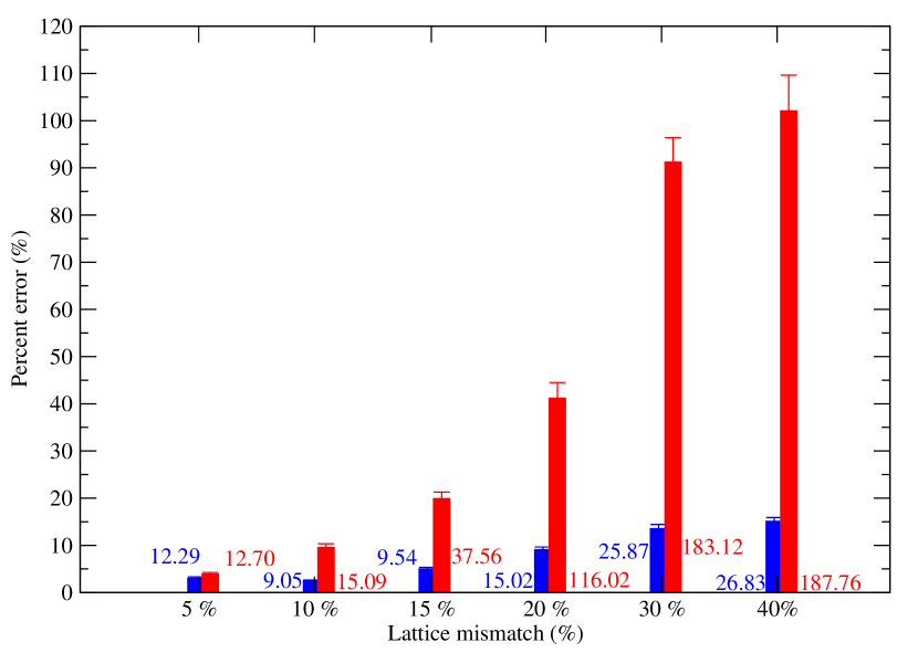
We computed the unrelaxed and relaxed using GULP and LAMMPS for FCC, BCC and HCP structures. Fig. S1 shows the fitting result of cluster expansion with Bayesian compression sensing. Cluster expansion can fit any unrelaxed energy computed from Lennard-Jones potential. All three unrelaxed crystals are within 1 to 2% prediction error. As the lattice mismatch increases, the predictive power of CE decreases (higher prediction errors and higher number of coefficients).

(a) Relaxation of FCC derivative structure

(b) Relaxation of HCP derivative structure

(c) Relaxation of BCC derivative structure

Figure S1: (color online) Cluster expansion fittings for a binary alloy using a Lennard-Jones potential. Blue bars represent the unrelaxed CE fits, while red bars show the relaxed CE fits. The colored numbers show the averaged number of coefficients for unrelaxed (in blue) and relaxed (in red) systems. As the lattice mismatch increases, the reliability of CE fits decreases.

VI.2.4 Stillinger-Weber

In addition to the LJ potential, we study the effect of relaxation using the Stillinger-Weber potential. Similar to the LJ potential, the Stillinger-Weber potential has a pair interaction but there is an additional angular (three-body) term. The parametric form of the SW potential is written as a sum of two-body and an anisotropic three-body interaction term as:

$$U=\sum_{\mathrm{pair}}\phi_{2}+\lambda\sum_{\mathrm{triplet}}\phi_{3}$$ (9)

Here $\phi_{2}$ depends only on the pair separation of atoms and $\phi_{3}$ depends on pair distances as well as angle formed by any three atoms and $\lambda$ controls the strength of the angular terms. Complete expressions for $\phi_{2}$ and $\phi_{3}$ can be given as [8]

$$\phi_{2}(r_{ij})=A\epsilon\left[B\left(\frac{\sigma}{r_{ij}}\right)^{p}-\left(\frac{\sigma}{r_{ij}}\right)^{q}\right]\exp\left(\frac{\sigma}{r_{ij}-a\sigma}\right),$$ (10)

$$\phi_{3}(r_{ij},r_{ik},\theta_{ijk})=\epsilon(\cos\theta_{ijk}-\cos\theta_{0})^{2}$$

$$\exp\left(\frac{\gamma\sigma}{r_{ij}-a\sigma}\right)\exp\left(\frac{\gamma\sigma}{r_{ik}-a\sigma}\right),$$ (11)

where the parameters are $A$ = 7.049556277, $B$ = 0.6022245584, $p$ = 4, $q$ = 0, $\gamma$ = 1.20 and $a$ = 1.80. We varied the $\lambda$ values from 0 to 1. Table S3 shows the parameters for a set of Stillinger-Weber potential. Similar to the LJ potential, the three systems have 5%, 10% and 15% lattice-mismatch. Additional modifications of Stillinger-Weber parameters are found in table S3. We performed extensive studies of the CE fit using SW potential. Some of the parameters are very similar or only vary by one or two parameters to examine the interaction strength, lattice mismatch, and angular dependence in the conditions that will lead to a myriad of relaxation. Additionally, we have a series of SW potentials where we varied the three-body contribution from 0 to 20 (see table S4). As we increased the $\lambda$ parameter, the relaxation is higher allowing us to map the CE fits in the highly relaxed configurations.

Table S3: SW parameters used to study the relaxation. $\epsilon$ is in eV and $\sigma$ is in unit of Å. $\lambda$ is equal to 0 (three-body contribution is off) or 1 (three-body contribution is on). System A, B and C are selected to show the effect of relaxation and to evaluate the relaxation metrics.

$\epsilon_{AA}$	$\sigma_{AA}$	$\epsilon_{BB}$	$\sigma_{BB}$	$\epsilon_{AB}$	$\sigma_{AB}$	$\theta$
0.21683	1.990	0.21683	2.1998	0.4336	2.0951	60
0.21683	1.938	0.21683	2.252	0.4336	2.0951	60
0.21683	2.0427	0.21683	2.1740	0.4336	2.0951	60
2.1683	2.0427	2.1683	2.1683	2.3813	2.0951	60
2.1683	2.0427	2.1683	2.1683	2.3813	2.0951	60
0.21683	2.0427	0.21683	2.1683	0.23813	2.0951	60
0.21683	2.0427	0.21683	2.1683	0.26020	2.0951	60
0.21683	2.0427	0.21683	2.1683	0.27103	2.0951	60
0.21683	2.0427	0.21683	2.1683	0.28188	2.0951	60
0.21683	2.0427	0.21683	2.1683	0.30356	2.0951	60
0.21683	2.0427	0.21683	2.1683	0.32525	2.0951	60
0.21683 (A)	2.0427	0.21683	2.1740	0.4336	2.0951	109.5
0.21683 (B)	1.990	0.21683	2.1998	0.4336	2.0951	109.5
0.21683 (C)	1.938	0.21683	2.252	0.4336	2.0951	109.5
2.1683	2.0427	2.1683	2.1683	2.3813	2.0951	109.5
2.1683	2.0427	2.1683	2.1683	2.3813	2.0951	109.5
0.21683	2.0427	0.21683	2.1683	0.23813	2.0951	109.5
0.21683	2.0427	0.21683	2.1683	0.26020	2.0951	109.5
0.21683	2.0427	0.21683	2.1683	0.27103	2.0951	109.5
0.21683	2.0427	0.21683	2.1683	0.28188	2.0951	109.5
0.21683	2.0427	0.21683	2.1683	0.30356	2.0951	109.5
0.21683	2.0427	0.21683	2.1683	0.32525	2.0951	109.5

Table S4: SW parameters used to study the relaxation with $\lambda$ varying from 0 (no interaction) to 20. $\epsilon$ is in eV and $\sigma$ is in unit of Å. $\lambda$ is three-body contribution where $\lambda$ equals zero they are no interaction and as $\lambda$ increases the three-body contribution is higher and higher relaxation.

$\epsilon_{AA}$	$\sigma_{AA}$	$\epsilon_{BB}$	$\sigma_{BB}$	$\epsilon_{AB}$	$\sigma_{AB}$	$\theta$
1.1683	1.990	2.80	2.1998	0.4336	2.0951	109.5
2.125	1.990	1.5285	2.200	3.0570	2.095	109.5

The Stillinger-Weber potential has several tunable parameters to simulate very high level of relaxations. CE fitting for BCC structures yields lower error than FCC or HCP as shown in table S5.

Table S5: Cluster expansion fittings using a Stillinger-Weber potential (system B in table S3) at 10% lattice mismatch.

Lattice	simulation	percent error (RMS/std(y) %)	$J$s
FCC	unrelaxed	0.07 %	3
FCC	relaxed	41.2 %	110
BCC	unrelaxed	0.03 %	3
BCC	relaxed	18.91 %	42
HCP	unrelaxed	0.23 %	4
HCP	relaxed	72.64 %	167

VI.2.5 Order Parameters (OPs)

In order to distinguish and measure the relaxation of the atoms from their ideal positions, we examined several metrics (order parameters) to quantify the relaxation: normalized mean-squared displacement or NMSD (see the method in the main article), Ackland’s order parameter [9], $D_{6}$, SOAP, and centro-symmetry. We found that some of these order parameters are not descriptive/general enough for all cases (potentials and crystal lattices).

We used the Ackland’s order parameter to identify the crystal structure after relaxation. Ackland’s OP identify each atomic local environment and assign it as FCC, BCC, HCP and Unknown [9]. We used this OP to determine which structures remain the same or on lattice and which structures undergo a structural change. We can use this order parameter to separate/sort those structure that remain the same to examine the robustness of CE due the relaxation of crystal structure. Similar to the Ackland’s order parameter, the centro-symmetry identifies the crystal structure of each atom based on the local arrangement (neighbors).

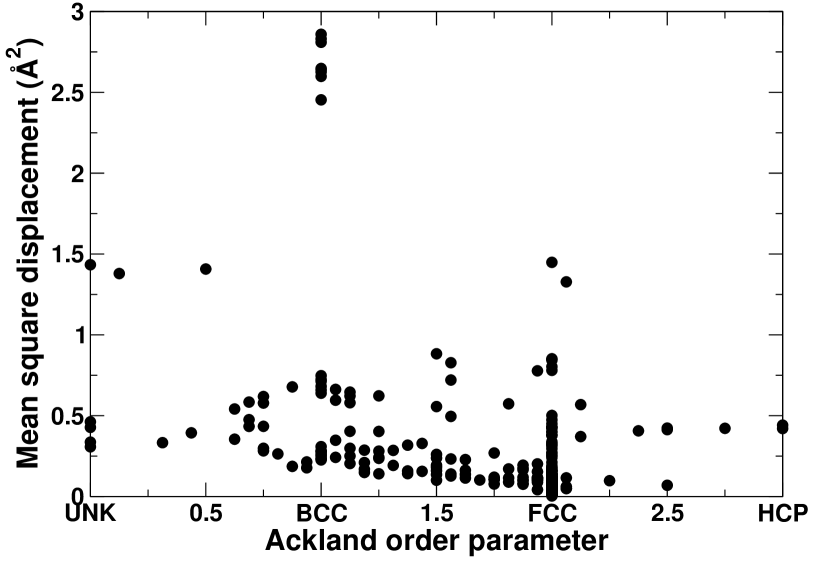
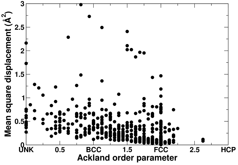
For example, Figure S2 shows the mapping of MSD and Ackland order parameter for each structure at 5% (top plot) and 15% (bottom plot). Overall, we can see that the MSD increases with higher lattice mismatch. The spread of the Ackland’s order parameter is also affected. Going from 5% (system A in table S3) to 15% (system C in table S3), the CE fitting error increases from 41.2% (110 clusters) to 63.5% (156 clusters) for the BCC. When the lattice mismatch increases, the mean-squared displacement also increases. Ackland’s order parameter and centro-symmetry are useful since they provide information about individual atoms. However, Ackland’s order parameter and centro-symmetry is too specific and it does not provide a useful measure of relaxation.

(a) 5% lattice mismatch

(b) 15% lattice mismatch

Figure S2: (color online) Mapping of structural changes and MSD for SW potential of a FCC lattice. The top panel shows the relaxation for a system with 5% lattice mismatch, while the bottom graph show relaxation of a 15% lattice mismatch system. Higher lattice mismatch equals higher mean-squared displacement.

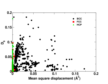
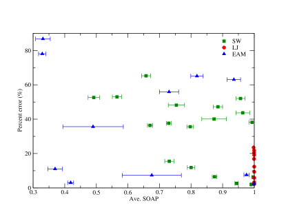
In addition to using the crystallographic information as a measure of relaxation, we used a variant of the Steinhardt’s bond order parameter [10] that we called the $D_{6}$ order parameter or the $D_{6}$ metric, which is a measure of the difference between the local atomic environment (relaxed and unrelaxed). We computed the local atomic environment using the $q_{6}$ (spherical harmonic with $l=6$) for the unrelaxed and relaxed configuration. We averaged the difference of the two configurations, $D_{6}=\frac{1}{N_{\mathrm{atom}}}\sum_{\mathrm{atom}}(q_{6,\mathrm{rel}}-q_{6,\mathrm{unrel}})$. Figure S3 shows the $D_{6}$ metric as a measure of relaxation vs the mean-squared displacement (MSD). We observe that $D_{6}$ metric does not correlate withe MSD. As relaxation increases (higher MSD), we expect that the $D_{6}$ value also increase. However, this metric is not robust for all systems, that is, we cannot compare the relaxation across all Hamiltonians (potentials and crystal lattices). Similar to the $D_{6}$ metrics, we used another metrics known as the SOAP (smooth overlap of atomic position) similarity kernel. The SOAP similarity kernel measures the difference in configuration (1 when it is identical and decreasing as the difference increases). The SOAP kernel is invariant to rotation and translation [11]; however, this metric is not applicable for multiple species cases. Fig. S4 shows the prediction error vs SOAP. Similar to $D_{6}$, the SOAP value does not correlate with the prediction error or displacement, that is, these metrics are too broad and vary too much for small displacements. This problem lies in the normalization of SOAP and $D_{6}$ values.

Figure S3: (color online) $D_{6}$ as a measure of the relaxation using a Lennard- Jones potential. We show that the $D_{6}$ metric does not correlated with the displacement. We show the relaxation of three crystal lattice. LJ favor FCC/ HCP; thus, we should not observe high relaxation (this is indicated by the displacement which is less than 0.001 $\mathrm{\AA^{2}}$. However, the $D_{6}$ metrics show a very broad range from 0.0 (identical configuration) up to 0.1. Although we only show this plot for LJ, the results of SW and EAM potential reveal the same conclusion, that is, $D_{6}$ is not a sufficient metric to analyze the various crystal lattices and potentials.

Figure S4: (color online) SOAP similarity kernel vs error. The plot shows the error as a function of the SOAP kernel. SOAP measure the similarity between the unrelaxed and relaxed configurations. When SOAP value is close to 1, the relaxed and unrelaxed configuration is similar (identical if it is 1). However, the plot shows that it is not a robust measure of relaxation as LJ has a very high range of prediction error for a very narrow range of SOAP value.

VI.3 Numerical Error

None of the normal quantifying descriptions of distribution shape (e.g., width, skewness, kurtosis, standard deviation, etc.) show a correlation with the CE prediction error. The error increased proportionally with the level of error in each system (2, 5, 10 and 15% error).

(a) Error vs Width

(b) Error vs Skewness

(c) Error vs Kurtosis

Figure S5: (color online) Width, skewness and kurtosis using the relaxation energies. The relaxation energies are obtained by taking the absolute difference of unrelaxed and relaxed energies. We show only the 2% and 15% error instead of all four error levels. This allows us to illustrate the effect of error level on the width, skewness and kurtosis of the distribution.

(a) Error vs Width

(b) Error vs Skewness

(c) Error vs Kurtosis

Figure S6: (color online) Width, skewness and kurtosis using total energies. The energies is the total relaxed energies. The green symbol represents the unrelaxed system.

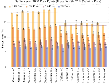
One other possibility is that the presence of outliers has a large impact on the performance of the BCS fit. To rule out that possibility, we performed fits with 0, 1, 2, 10, 20, 30, 40, 50 and 60 outliers added to the error (representing between 0 and 3% of the total data). Outliers were selected randomly from between 2 and 4 standard deviations from the mean and then appended to the regular list of errors drawn from the distribution (the total number of values equaling 2000 again to match the number of structures). The summary is plotted in Figure S7. The difference between fits as the number of outliers changes is comparable to the variance in the individual fits. We conclude then that outliers have no direct effect on the error profile’s performance.

Figure S7: (color online) Fitting errors as outliers are added to the error profile. The difference between fits as the number of outliers changes is comparable to the variance in the individual fits.

VI.4 Evolution of $J$ Coefficients on Relaxation

To further elucidate the claims relative to the CE framework’s failures, we investigated whether we could measure the change in configuration upon relaxation. Since the $J$ values selected in the model are backed by geometric clusters, the presence or absence of certain clusters has some correlation to the configuration of the physical system. When the physics is mostly dependent on configuration, the function can be sparsely represented by the CE basis. Thus, we expect that the sparsity will be a good heuristic in determining when the CE breaks down. When the expansion terms do not decay well in the representation, it shows a misapplication of the CE basis to a problem that is not mostly configurational.

We define three new quantities:

1. $\Xi$: total number of unique clusters used over 100 CE fits of the same dataset. We also call this the model complexity as shown in Fig. S8.

2. $\not\in$: number of “exceptional” clusters. These are clusters that show up fewer than 25 times across 100 fits, implying that they are not responsible for representing any real physics in the signal, but are rather included because the CE basis is no longer a sparse representation for the relaxed alloy system (shown in Fig. S9. It is sensitive to the training subsets.

3. $\Lambda$: number of significant clusters in the fit; essentially just the total number of unique clusters minus the number of “exceptional” clusters, $\Lambda=\Xi-\not\in$ (see Fig. S10).

(a) 2% error added

(b) 5% error added

(c) 10% error added

(d) 15% error added

Figure S8: (color online) Prediction error over 65% of the structures for the toy CE system. The systems are ordered by $\Xi$, which is the total number of unique clusters used by any of the 100 CE fits for the system. This ordering shows a definite trend with increasing $\Xi$.

(a) 2% error added

(b) 5% error added

(c) 10% error added

(d) 15% error added

Figure S9: (color online) Plot of predictive error over 65% of the structures for the toy model. The systems are ordered by $\not\in$ the number of clusters that were used less than 25 times across all 100 CE fits. These are considered exceptions to the overall fit for the system. As for Figure S8, there is a definite trend toward higher error for systems with more cluster exceptions. When $\not\in$ is equal to zero, CE only uses the significant terms.

(a) 2% error added

(b) 5% error added

(c) 10% error added

(d) 15% error added

Figure S10: (color online) Prediction error over 65% of the structures with the toy CE model. The errors are ordered by $\Lambda$, the number of significant terms in the expansion. As expected, the values are close to the known model complexity (5 terms) and the ordering once more appears random.

Fig. S8, S9, S10 display the additional plots at different error level that were not shown in the main text.

VI.5 References

References

- [1] J. M. Sanchez, F. Ducastelle, and D. Gratias. Generalized cluster description of multicomponent systems. Physica A: Statistical and Theoretical Physics, 128(1-2):334–350, 1984.
- [2] J. M. Sanchez. Cluster expansions and the configurational energy of alloys. Physical Review B, 48(18):14013–14015, nov 1993.
- [3] J. M. Sanchez. Cluster expansion and the configurational theory of alloys. Physical Review B, 81(22):224202, jun 2010.
- [4] J. W D Connolly and a. R. Williams. Density-functional theory applied to phase transformations in transition-metal alloys. Physical Review B, 27(8):5169–5172, apr 1983.
- [5] L. G. Ferreira, A A Mbaye, and Alex Zunger. Effect of chemical and elastic interactions on the phase diagrams of isostructural solids. Physical Review B, 35(12):6475–6478, apr 1987.
- [6] L. G. Ferreira, A. A. Mbaye, and A. Zunger. Chemical and elastic effects on isostructural phase diagrams: The e-G approach. Physical Review B, 37(18):10547, 1988.
- [7] L. G. Ferreira, S.-H. Wei, and A. Zunger. First-principles calculation of alloy phase diagrams: The renormalized-interaction approach. Physical Review B, 40(5):3197, 1989.
- [8] Z. W. Lu, S.-H. H. Wei, Alex Zunger, S. Frota-Pessoa, and L. G. Ferreira. First-principles statistical mechanics of structural stability of intermetallic compounds. Physical Review B, 44(2):512–544, 1991.
- [9] C Wolverton and A Zunger. Ni-Au: A testing ground for theories of phase stability. Computational Materials Science, 8(1-2):107–121, 1997.
- [10] A. van de Walle and G. Ceder. Automating first-principles phase diagram calculations. Journal of Phase Equilibria, 23(4):348–359, aug 2002.
- [11] Sergey V. Barabash, Volker Blum, Stefan Müller, and Alex Zunger. Prediction of unusual stable ordered structures of Au-Pd alloys via a first-principles cluster expansion. Physical Review B, 74(3):035108, jul 2006.
- [12] M Asato, H Takahashi, T Inagaki, N Fujima, R Tamura, and T Hoshino. Cluster Expansion Approach for Relative Stability among Different Atomic Structures in Alloys: an Approach from a Dilute Limit. MATERIALS TRANSACTIONS, 48(7):1711–1716, 2007.
- [13] Lance J. Nelson, Vidvuds Ozoliņš, C. Shane Reese, Fei Zhou, and Gus L. W. Hart. Cluster expansion made easy with Bayesian compressive sensing. Physical Review B, 88(15):155105, 2013.
- [14] P.H. Gargano, P.R. Alonso, and G.H. Rubiolo. Ordering in the Solid Solution U(Al,Si)3. Procedia Materials Science, 9:239–245, 2015.
- [15] Manuel Aldegunde, Nicholas Zabaras, and Jesper Kristensen. Quantifying uncertainties in first-principles alloy thermodynamics using cluster expansions. Journal of Computational Physics, (July), 2016.
- [16] Ravi Chinnappan, B.K. Panigrahi, and Axel van de Walle. First-principles study of phase equilibrium in Ti–V, Ti–Nb, and Ti–Ta alloys. Calphad, 54:125–133, 2016.
- [17] G Ceder, a Van Der Ven, C Marianetti, and D Morgan. First-principles alloy theory in oxides. Modelling and Simulation in Materials Science and Engineering, 8:311–321, 2000.
- [18] Atsuto Seko, Koretaka Yuge, Fumiyasu Oba, Akihide Kuwabara, and Isao Tanaka. Prediction of ground-state structures and order-disorder phase transitions in II-III spinel oxides: A combined cluster-expansion method and first-principles study. Physical Review B - Condensed Matter and Materials Physics, 73(18):1–5, 2006.
- [19] Atsuto Seko, Atsushi Togo, Fumiyasu Oba, and Isao Tanaka. Structure and stability of a homologous series of tin oxides. Physical Review Letters, 100(4):2–5, 2008.
- [20] Isao Tanaka, Atsushi Togo, Atsuto Seko, Fumiyasu Oba, Yukinori Koyama, and Akihide Kuwabara. Thermodynamics and structures of oxide crystals by a systematic set of first principles calculations. Journal of Materials Chemistry, 20(46):10335, 2010.
- [21] Isao Tanaka, Atsuto Seko, Atsushi Togo, Yukinori Koyama, and Fumiyasu Oba. Phase relationships and structures of inorganic crystals by a combination of the cluster expansion method and first principles calculations. Journal of physics. Condensed matter : an Institute of Physics journal, 22(38):384207, 2010.
- [22] Stefan Müller. Bulk and surface ordering phenomena in binary metal alloys. Journal of Physics: Condensed Matter, 15(34):R1429–R1500, 2003.
- [23] Ralf Drautz, R Singer, and M Fähnle. Cluster expansion technique: An efficient tool to search for ground-state configurations of adatoms on plane surfaces. Physical Review B, 67(3):035418, 2003.
- [24] S. Müller, M. Stöhr, and O. Wieckhorst. Structure and stability of binary alloy surfaces: Segregation, relaxation, and ordering from first-principles calculations. Applied Physics A: Materials Science and Processing, 82(3 SPEC. ISS.):415–419, 2006.
- [25] Laura M. Herder, Jason M. Bray, and William F. Schneider. Comparison of cluster expansion fitting algorithms for interactions at surfaces. Surface Science, 640:104–111, 2015.
- [26] Ryohei Tanaka, Kazuhito Takeuchi, and Koretaka Yuge. Application of Grid Increment Cluster Expansion to Modeling Potential Energy Surface of Cu-Based Alloys. Materials Transactions, 56(7):1077–1080, 2015.
- [27] David B. Laks, L. G. Ferreira, Sverre Froyen, and Alex Zunger. Efficient cluster expansion for substitutional systems. Physical Review B, 46(19):12587–12605, nov 1992.
- [28] Bjoern Arnold, Alejandro Diaz Ortiz, Gus L W Hart, and Helmut Dosch. Structure-property maps and optimal inversion in configurational thermodynamics. Phys. Rev. B, 81(9):1–11, 2010.
- [29] Alejandro Díaz-Ortiz and Helmut Dosch. Noise filtering of cluster expansions in multicomponent systems. Physical Review B, 76(1):012202, jul 2007.
- [30] Alejandro Díaz-Ortiz, Helmut Dosch, and Ralf Drautz. Cluster expansions in multicomponent systems: precise expansions from noisy databases. Journal of Physics: Condensed Matter, 19:406206, 2007.
- [31] S. M. Foiles, M. I. Basker, and M. S. Daw. Embedded-atom-method functions for the fcc meatls Cu, Ag, Au, Ni, Pd, Pt, and their alloys. Physical Review B, 33(12), 1986.
- [32] Frank H. Stillinger and Thomas a. Weber. Computer simulation of local order in condensed phases of silicon. Physical Review B, 31(8):5262–5271, 1985.
- [33] G. Kresse and J. Hafner. Ab initio molecular dynamics for liquid metals. Physical Review B, 47(1):558–561, 1993.
- [34] G. Kresse and J. Hafner. Ab initio molecular-dynamics simulation of the liquid-metal–amorphous-semiconductor transition in germanium. Physical Review B, 49(20):14251–14269, 1994.
- [35] G. Kresse and J. Furthmüller. Efficiency of ab-initio total energy calculations for metals and semiconductors using a plane-wave basis set. Computational Materials Science, 6(1):15–50, 1996.
- [36] G. Kresse and J. Furthmüller. Efficient iterative schemes for ab initio total-energy calculations using a plane-wave basis set. Physical Review B, 54(16):11169–11186, 1996.
- [37] P. E. Blöchl. Projector augmented-wave method. Physical Review B, 50(24):17953–17979, dec 1994.
- [38] John P. Perdew, Kieron Burke, Matthias Ernzerhof, Department of Physics, and New Orleans Louisiana 70118 John Quantum Theory Group Tulane University. Generalized Gradient Approximation Made Simple. Physical Review Letters, 77(18):3865–3868, 1996.
- [39] Sverre Froyen. Brillouin-zone integration by Fourier quadrature: Special points for superlattice and supercell calculations. Physical Review B, 39(5):3168–3172, feb 1989.
- [40] Julian D. Gale. GULP: A computer program for the symmetry-adapted simulation of solids. J. Chem. Soc., Faraday Trans., 93(4):629–637, 1997.
- [41] Julian D. Gale and Andrew L. Rohl. The General Utility Lattice Program (GULP). Molecular Simulation, 29(5):291–341, may 2003.
- [42] S. Plimpton. Fast Parallel Algorithms for Short – Range Molecular Dynamics. Journal of Computational Physics, 117(June 1994):1–19, 1995.
- [43] See supplemental materials for details about the different potentials and their parameters.
- [44] Gus L. W. Hart and Rodney W. Forcade. Algorithm for generating derivative structures. Physical Review B, 77(22):1–12, 2008.
- [45] Gus L W Hart and Rodney W. Forcade. Generating derivative structures from multilattices: Algorithm and application to hcp alloys. Physical Review B - Condensed Matter and Materials Physics, 80(1):1–8, 2009.
- [46] D Lerch, O Wieckhorst, G L W Hart, R W Forcade, and S Müller. UNCLE: a code for constructing cluster expansions for arbitrary lattices with minimal user-input. Modelling and Simulation in Materials Science and Engineering, 17(5):055003, sep 2009.
- [47] See supplemental materials for more details on cluster expansion.
- [48] L.G. Ferreira, S.-H. Wei, and Alex Zunger. Stability, Electronic Structure, and Phase Diagrams of Novel Inter- Semiconductor Compounds. International Journal of High Performance Computing Applications, 5(1):34–56, mar 1991.
- [49] Alex Zunger, L G Wang, Gus L W Hart, and Mahdi Sanati. Obtaining Ising-like expansions for binary alloys from first principles. Modelling and Simulation in Materials Science and Engineering, 10(6):685–706, 2002.
- [50] Axel van de Walle. Methods for First-Principles Alloy Thermodynamics. JOM, 65(11):1523–1532, nov 2013.
- [51] Lance J. Nelson, Gus L. W. Hart, Fei Zhou, and Vidvuds Ozoliņš. Compressive sensing as a paradigm for building physics models. Physical Review B, 87(3):035125, 2013.
- [52] Emmanuel J. Candes and Terence Tao. Near-Optimal Signal Recovery From Random Projections: Universal Encoding Strategies? IEEE Transactions on Information Theory, 52(12):5406–5425, dec 2006.
- [53] E.J. Candes and M.B. Wakin. An Introduction To Compressive Sampling. IEEE Signal Processing Magazine, 25(2):21–30, mar 2008.
- [54] G. J. Ackland and a. P. Jones. Applications of local crystal structure measures in experiment and simulation. Physical Review B, 73(5):054104, feb 2006.
- [55] Paul J. Steinhardt, David R. Nelson, and Marco Ronchetti. Bond-orientational order in liquids and glasses. Physical Review B, 28(2):784–805, jul 1983.
- [56] Albert P. Bartók, Risi Kondor, and Gábor Csányi. On representing chemical environments. Physical Review B - Condensed Matter and Materials Physics, 87(18):1–16, 2013.
- [57] Cynthia L. Kelchner, S. J. Plimpton, and J. C. Hamilton. Dislocation nucleation and defect structure during surface indentation. Physical Review B, 58(17):11085–11088, nov 1998.
- [58] See supplemental materials for details about the different relaxation metrics.
- [59] In our experience, a percent error above 10% often gives unreliable CE model.
- [60] See supplemental materials for additional plots at different levels of error.
- [61] The supplementary data has many plots from the hundreds of CE fits that we performed for this analysis.
- [62] For typical binary CEs we typically need about 300-500 structures to get a good fit, which is then verified using an additional 200+ DFT calculations.
- [1] J. W D Connolly and a. R. Williams. Density-functional theory applied to phase transformations in transition-metal alloys. Physical Review B, 27(8):5169–5172, apr 1983.
- [2] Lance J. Nelson, Vidvuds Ozoliņš, C. Shane Reese, Fei Zhou, and Gus L. W. Hart. Cluster expansion made easy with Bayesian compressive sensing. Physical Review B, 88(15):155105, 2013.
- [3] Lance J. Nelson, Gus L. W. Hart, Fei Zhou, and Vidvuds Ozoliņš. Compressive sensing as a paradigm for building physics models. Physical Review B, 87(3):035125, 2013.
- [4] Julian D. Gale. GULP: A computer program for the symmetry-adapted simulation of solids. J. Chem. Soc., Faraday Trans., 93(4):629–637, 1997.
- [5] Julian D. Gale and Andrew L. Rohl. The General Utility Lattice Program (GULP). Molecular Simulation, 29(5):291–341, may 2003.
- [6] S. Plimpton. Fast Parallel Algorithms for Short – Range Molecular Dynamics. Journal of Computational Physics, 117(June 1994):1–19, 1995.
- [7] S. M. Foiles, M. I. Basker, and M. S. Daw. Embedded-atom-method functions for the fcc meatls Cu, Ag, Au, Ni, Pd, Pt, and their alloys. Physical Review B, 33(12), 1986.
- [8] Frank H. Stillinger and Thomas a. Weber. Computer simulation of local order in condensed phases of silicon. Physical Review B, 31(8):5262–5271, 1985.
- [9] G. J. Ackland and a. P. Jones. Applications of local crystal structure measures in experiment and simulation. Physical Review B, 73(5):054104, feb 2006.
- [10] Paul J. Steinhardt, David R. Nelson, and Marco Ronchetti. Bond-orientational order in liquids and glasses. Physical Review B, 28(2):784–805, jul 1983.
- [11] Albert P. Bartók, Risi Kondor, and Gábor Csányi. On representing chemical environments. Physical Review B - Condensed Matter and Materials Physics, 87(18):1–16, 2013.