The $\Lambda$-parameter in 3-flavour QCD and $\alpha_{s}(m_{Z})$ by the ALPHA collaboration

Abstract:

We present results by the ALPHA collaboration for the $\Lambda$-parameter in 3-flavour QCD and the strong coupling constant at the electroweak scale, $\alpha_{s}(m_{Z})$, in terms of hadronic quantities computed on the CLS gauge configurations. The first part of this proceedings contribution contains a review of published material [1, 2] and yields the $\Lambda$-parameter in units of a low energy scale, $1/L_{\rm had}$. We then discuss how to determine this scale in physical units from experimental data for the pion and kaon decay constants. We obtain $\Lambda_{\rm\overline{MS\kern-0.35002pt}\kern 0.35002pt}^{(3)}=332(14)\,{\rm MeV}$ which translates to $\alpha_{s}(M_{Z})=0.1179(10)(2)$ using perturbation theory to match between 3-, 4- and 5-flavour QCD.

CERN-TH-2016-262

DESY 17-007

1 Introduction

The strong coupling in QCD is a fundamental parameter of the Standard Model and its precise knowledge is both of principal importance and of practical relevance to LHC physics. We here report on the ALPHA collaboration’s results for the $\Lambda$-parameter in 3-flavour QCD and $\alpha_{s}(m_{Z})$. The project was designed to match hadronic quantities computed on CLS gauge configurations for 3-flavour QCD at low energies [3, 4]. The strategy for the $\Lambda$-parameter was explained in [5, 6] and relies on the methods and tools developed over many years (see [7, 8] and references therein). As a result we are able to defer the use of perturbation theory in 3-flavour QCD to high energies of O(100 GeV). On the other hand, the determination of $\alpha_{s}(m_{Z})$ requires the matching to the 4- and 5-flavour theories across the charm and bottom quark thresholds which still relies on perturbation theory [9, 10]. At all stages the continuum limit is taken and rather well controlled. Our strategy combines the perturbative knowledge of the standard SF coupling at high energies with the advantageous properties of finite volume gradient flow couplings at low energies. A non-perturbative matching between these 2 coupling schemes is performed at an intermediate scale $1/L_{0}\approx 4\,{\rm GeV}$. At the largest box size reached, $L_{\rm had}$, the matching to the gradient flow time scale $t_{0}^{\ast}$ at the SU(3) symmetric point is performed. Together with the recent results of ref. [4] (which rely on a new high precision determination of the axial current normalization constant [11], based on the method in [12]), this allows us to accurately relate to a linear combination of pion and kaon decay constants and thus express all results in physical units.

In this write-up we go through the different steps of this strategy starting from the high energy end (section 2). The connection between the intermediate scale $L_{0}$ and $L_{\rm had}$ is discussed in section 3, including the matching at scale $L_{0}$. Relating $L_{\rm had}$ to a hadronic scale is the subject of section 4. This allows to quote the 3-flavour $\Lambda$-parameter in physical units. The perturbative connection to 5-flavour QCD is carried out in section 5, followed by our conclusions. Finally, a technical point pertaining to the interpolation of the low energy data is relegated to an appendix. Note that the first 2 steps have been published in [1] and [2], respectively. Further details on the first step will be given elsewhere [13]. The matching of $L_{\rm had}$ to a hadronic scale is currently being finalized. For a recent account aimed at a non-lattice audience we refer to [14].

2 The high energy regime

2.1 A family of couplings in the SF scheme

Using the Schrödinger functional in QCD [15, 16], the spatial vector components of the gauge field at the time boundaries $x_{0}=0,T$ are taken to be spatially constant and Abelian [17],

$$A_{k}(x)\big{|}_{x_{0}=0}=C_{k} = \dfrac{i}{L}{\rm diag}\left(\eta-\frac{\pi}{3},\eta\left(\nu-\frac{1}{2}\right),-\eta\left(\nu+\frac{1}{2}\right)+\frac{\pi}{3}\right),$$ (1a)

$$A_{k}(x)\big{|}_{x_{0}=T}=C_{k}^{\prime} = \dfrac{i}{L}{\rm diag}\left(-\pi-\eta,\eta\left(\nu+\frac{1}{2}\right)+\frac{\pi}{3},-\eta\left(\nu-\frac{1}{2}\right)+\frac{2\pi}{3}\right),$$ (1b)

for $k=1,2,3$. The parameters $\eta$ and $\nu$ correspond with the existence of 2 abelian generators in SU(3). The absolute minimum of the action with these boundary values is attained for [15]

$$B_{k}(x)=C_{k}+\dfrac{x_{0}}{T}\left(C_{k}^{\prime}-C_{k}\right),\qquad B_{0}=0\,,$$ (2)

the induced background field, which is unique up to gauge equivalence. The effective action of the Schrödinger functional $\Gamma[B]$ is then unambiguously defined and its perturbative expansion straightforward in principle,

$$\Gamma[B]=\frac{1}{g_{0}^{2}}\Gamma_{0}[B]+\Gamma_{1}[B]+{\rm O}(g_{0}^{2}),$$ (3)

with the first term given by the classical action of the background field,

$$\Gamma_{0}[B]=g_{0}^{2}S[B]=2(\pi+3\eta)^{2}\,.$$ (4)

Setting all quark masses to zero and $T=L$, the only remaining scale is set by $L$. The SF coupling at this scale is then defined as a derivative with respect to a background field parameter,

$$\left.\dfrac{\partial_{\eta}\Gamma[B]}{\partial_{\eta}\Gamma_{0}[B]}\right|_{\eta=0}=\dfrac{\left.\left\langle\partial_{\eta}S\right\rangle\right|_{\eta=0}}{12\pi}=\dfrac{1}{\bar{g}^{2}(L)}-\nu\times\bar{v}(L)\,.$$ (5)

The derivative produces an expectation value which can be measured in numerical simulations. In fact, there are 2 observables, the inverse coupling $1/\bar{g}^{2}(L)$ and $\bar{v}(L)$ both of which are measured at $\nu=0$. A new feature of our project is the re-interpretation of the parameter $\nu$ as index of a family of SF couplings,

$$\dfrac{1}{\bar{g}_{\nu}^{2}(L)}=\dfrac{1}{\bar{g}^{2}(L)}-\nu\times\bar{v}(L)\,.$$ (6)

This has first been envisaged as a method to reduce large cutoff effects in strongly coupled models of electroweak symmetry breaking in [18].

In perturbation theory the $\beta$-function of the SF coupling family is known to 3-loops from the 2-loop matching to the $\overline{\rm MS}$-coupling in [19, 20, 21, 22] combined with the knowledge of the $\beta$-function in the $\overline{\rm MS}$-scheme (cf. [23, 24] and references therein),

$$\beta(\bar{g}_{\nu})=-L\frac{\partial\bar{g}_{\nu}(L)}{\partial L}=-b_{0}\bar{g}_{\nu}^{3}-b_{1}\bar{g}_{\nu}^{5}-b_{2,\nu}\bar{g}_{\nu}^{7}+{\rm O}(\bar{g}_{\nu}^{9})\,.$$ (7)

In 3-flavour QCD the universal terms are $b_{0}=9/(4\pi)^{2}$ and $b_{1}=1/(4\pi^{4})$. The 3-loop coefficient is then found to be

$$b_{2,\nu}=\left(-0.06(3)-\nu\times 1.26\right)/(4\pi)^{3}\,.$$ (8)

The $\Lambda$-parameter in the ${\rm SF}_{\nu}$ scheme is defined by

$$L\Lambda_{{\rm SF}_{\nu}}=\varphi_{\nu}\left(\bar{g}_{\nu}(L)\right)=\big{[}{b_{0}\bar{g}_{\nu}^{2}(L)}\big{]}^{-\frac{b_{1}}{2b_{0}^{2}}}\,{\rm e}^{-\frac{1}{{2b_{0}\bar{g}_{\nu}^{2}(L)}}}\exp\bigg{\{}-\int_{0}^{\bar{g}_{\nu}(L)}\!dg\bigg{[}\dfrac{1}{\beta(g)}+\dfrac{1}{b_{0}g^{3}}-\dfrac{b_{1}}{b_{0}^{2}g}\bigg{]}\bigg{\}}\,.$$ (9)

When evaluating the $\Lambda$-parameter one would like to know from which scale $L$ one can trust perturbation theory to evaluate the integral in the exponent and how one can quantify the associated systematic error. We proceed as follows: first we fix a reference scale, $L_{0}$, through

$$\bar{g}^{2}(L_{0})=2.012,$$ (10)

and use the step-scaling function (cf. next subsection) to step up the energy scale non-perturbatively by factors of 2 from $L_{0}$ to $L_{n}=L_{0}/2^{n}$, for $n=0,1,2,\ldots$. We then use the $\nu=0$ $\Lambda_{\rm SF}$-parameter as reference point and consider

$$L_{0}\Lambda_{\rm SF}=\underbrace{(\Lambda_{\rm SF}/\Lambda_{{\rm SF}_{\nu}})}_{\exp(-\nu\times 1.25516)}\times\underbrace{(L_{0}/L_{n})}_{2^{n}}\times\varphi_{\nu}(\bar{g}_{\nu}(L_{n}))$$ (11)

with $\varphi_{\nu}(\bar{g}_{\nu}(L_{n}))$ evaluated in perturbation theory, by inserting the value of the coupling $\bar{g}_{\nu}^{2}(L_{n})$ obtained non-perturbatively from the step-scaling procedure and the 3-loop truncated $\beta$-function. Up to perturbative errors of order $\alpha^{2}(1/L_{n})=\bar{g}_{\nu}^{4}(L_{n})/(4\pi)^{2}$, the result for $L_{0}\Lambda$ must be independent of the number of steps $n$ and the value of the parameter $\nu$. This gives us an excellent control over the remaining systematic error stemming from perturbation theory. Before discussing the result we briefly present some key features of our numerical simulations, the measurements and the data analysis.

2.2 Numerical simulation data and analysis

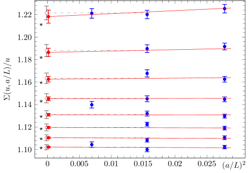
Figure 1: Continuum extrapolation of the step scaling function. The leftmost points are the continuum values, whereas the stars are obtained from perturbative scale evolution using the 3-loop $\beta$-function.

For the simulation at high energies we choose the Wilson plaquette action in order to use 2-loop perturbative information at finite $L/a$ which is only available for this regularization [19]. This allows for more control of boundary O($a$) effects and also for perturbative improvement of the non-perturbative data of the step-scaling function. We use the result for $c_{\rm sw}$ from [25]. A very careful tuning of the bare mass parameters to their critical values in [26] reduces associated systematics to negligible levels. All our simulations have been carried out with a modification of the openQCD code [27]. Compared to earlier studies of the SF coupling in 3-flavour QCD in [28] (there with the Iwasaki gauge action), we have significantly reduced statistical errors. We have produced data for the step-scaling functions

$$\Sigma_{\nu}(u,a/L)=\bar{g}_{\nu}^{2}(2L)|_{\bar{g}_{\nu}^{2}(L)=u,m(L)=0}\,,$$ (12)

for lattice resolutions $L/a=6,8,12$ and the corresponding doubled lattice sizes. For $\nu=0$ our data corresponds to $u$-values in the interval $[1.1,2.0]$. Cutoff effect are O($a^{2}$) in the bulk, and O($a$) from the time boundaries. The latter are governed by 2 counterterms of dimension 4 with coefficients $c_{\rm t}$ and $\tilde{c}_{\rm t}$, known to 2-loop [19] and 1-loop order [29] respectively. Using these perturbative results for the coefficients we expect that O($a$) effects are strongly reduced. As a safeguard against any O($a$) contamination of our continuum extrapolations we include a systematic error as follows. We determine the $c_{\rm t}$ and $\tilde{c}_{\rm t}$ derivatives of the coupling numerically by a variation in a few points and, together with the corresponding perturbative information arrive at a model for the sensitivity of our data to such variations. We then use the last known perturbative coefficients for $c_{\rm t}$ and $\tilde{c}_{\rm t}$ as an uncertainty and add the corresponding systematic error to the data. Note that this is likely an overestimate of the true error [13]. Fig. 1 shows our data points for the step-scaling function at $\nu=0$. We then perform global fits of the data, for example

$$\Sigma^{(2)}(u,a/L)=u+s_{0}u^{2}+s_{1}u^{3}+{c_{1}}u^{4}+{c_{2}}u^{5}+{\rho_{1}}u^{4}\dfrac{a^{2}}{L^{2}}+{\rho_{2}}u^{5}\dfrac{a^{2}}{L^{2}}\,,$$ (13)

where $\Sigma^{(2)}$ denotes the 2-loop improved non-perturbative data, such that cutoff effects appear, by construction, first at O($u^{4}$) [30]. The coefficients $s_{0}$, $s_{1}$ are fixed to their perturbative values,

$$s_{0}=2b_{0}\ln 2,\quad s_{1}=s_{0}^{2}+2b_{1}\ln 2\,,$$ (14)

and we thus obtain the non-perturbative continuum step-scaling function $\sigma(u)$ in terms of the fit coefficients $c_{1}$ and $c_{2}$ and their correlation, as required for the error propagation.

2.3 Results for $L_{0}\Lambda$

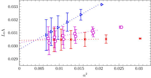
Figure 2: The extraction of the $\Lambda$-parameter using perturbation theory at different values of $\alpha$, plotted vs. $\alpha^{2}(1/L_{n})$. The data points are, from top to bottom, for $\nu=-0.5,0,0.3$ and, from right to left, for $n=0,1,\ldots,5$ steps by a factor 2 in scale.

Given the step-scaling functions in the continuum limit our data allows us to take up to $n=5$ steps from $L_{0}$, thus covering a factor of $2^{5}=32$ in scale. For $\nu\neq 0$ one also needs to know the value of $\bar{v}$ at $L_{0}$ [1],

$$\bar{v}(L_{0})=0.1199(10)\,.$$ (15)

We have considered O(10) $\nu$-values around $\nu=0$. We present data for $\nu=0.3$ and $\nu=-0.5$ besides the reference choice $\nu=0$. Fig. 2 shows the corresponding $3\times 6$ data points for $L_{0}\Lambda$ from eq. (9), each corresponding to a determination of $L_{0}\Lambda$ using non-perturbative data between $L_{0}$ and $L_{n}$ and perturbation theory for $L<L_{n}$. As can be seen in the plot the data points nicely come together at small $L$ (high energy scales) where $\alpha(1/L_{n})\approx 0.1$. We are therefore confident to quote our result with an error of $3\%$,

$$L_{0}\Lambda_{\rm SF}=0.0303(8)\quad\Leftrightarrow\quad L_{0}\Lambda_{\rm\overline{MS\kern-0.35002pt}\kern 0.35002pt}^{(3)}=0.0791(21)\,,$$ (16)

which is the main result of our study of the large energy region. In a recent letter [1] we have also presented a by-product of this study, namely the observation that renormalized perturbation theory in continuum QCD might be susceptible to larger systematic errors than often assumed. This is apparent in fig. 2 and in the continuum result for $\bar{v}(L)$ where perturbation theory at $\alpha=0.19$ does not look trustworthy. This is particularly worrisome given the very advantageous properties of the ${\rm SF}_{\nu}$-schemes in perturbation theory [1, 13].

3 Connecting with hadronic scales

In the previous section we have detailed our very accurate matching with perturbation theory. The result is given in eq. (16) and relates the $\Lambda$-parameter with $L_{0}$, defined implicitly through $\bar{g}^{2}_{\rm SF}(L_{0})=2.012$. The corresponding energy scale, $1/L_{0}\approx 4{\rm GeV}$, is still very large if one aims at using lattice methods to study continuum properties of QCD while having finite volume effects under control. Therefore we will continue using our finite size scaling technique in order to relate the scale $L_{0}$ with a scale $L_{\rm had}$ characteristic of hadronic physics.

In principle one could simply continue with the program explained in the previous section until reaching the energy scale $1/L_{\rm had}$. Unfortunately the statistical precision of the SF coupling deteriorates very fast when reaching large volumes (see for example the discussion in [31] and references therein), making it very difficult to maintain the precision. In order to overcome these problems we will continue to work with a finite volume renormalization scheme, but we will use the gradient flow coupling in a finite volume with SF boundary conditions [32] for our running coupling. Renormalized couplings based on the gradient flow have the nice property that their variance is roughly independent of the lattice spacing.

The main result of this section [2] is the precise determination of the ratio of two scales

$$L_{\mathrm{had}}/L_{0}=21.86(42)\quad\text{for}\quad\bar{g}^{2}_{\rm GF}(L_{\mathrm{had}})=11.31\,.$$ (17)

Note, however, that in the usual step scaling procedure (see previous section) the aim is to determine the value of the renormalized coupling at two scales $L_{1}$ and $L_{2}$ that are separated by an integer power of the scale factor (i.e. $L_{1}=2^{n}L_{2}$ with $n\in\mathbb{Z}$ when the scale factor is $s=2$). Here we need to solve a slightly different problem: we know the value of the coupling at two scales ($L_{0}$ and $L_{\rm had}$), and are interested in computing the ratio of these scales. With our conventions, the $\beta$-function is defined by

$$-L\frac{\partial\bar{g}_{\rm GF}(L)}{\partial L}=\beta(\bar{g}_{\rm GF})\,,$$ (18)

and ratios of scales such as (17) can be easily computed, once the $\beta$-function is known, thanks to the relation

$$\frac{L_{1}}{L_{2}}=\exp\left\{-\int_{\bar{g}_{\rm GF}(L_{2})}^{\bar{g}_{\rm GF}(L_{1})}\frac{dx}{\beta(x)}\right\}\,.$$ (19)

In order to determine the $\beta$-function, we will first determine the usual continuum step scaling function,

$$\sigma_{\rm GF}(u)=\bar{g}^{2}_{\rm GF}(2L)\Big{|}_{g^{2}_{\rm GF}(L)=u}\,,$$ (20)

and use it to constrain the functional form of $\beta(g)$ by using the exact relation

$$\log 2=-\int_{\sqrt{u}}^{\sqrt{\sigma_{\rm GF}(u)}}\frac{dx}{\beta(x)}\,.$$ (21)

3.1 Coupling definition and choices of discretization

The gradient flow coupling with SF boundaries conditions has been studied in [32], and the interested reader should consult the cited reference. We impose SF boundary conditions with zero background field (i.e. $C_{k}=C_{k^{\prime}}=0$ in eq. (1)). The gradient flow [33, 34] determines how the gauge field $B_{\mu}(t,x)$ evolves with the flow time $t$ (not to be confused with the Euclidean time $x_{0}$) via the (non-linear) diffusion-like equation

$$\frac{\partial B_{\mu}(t,x)}{\partial t}=D_{\nu}G_{\nu\mu}(t,x);\quad A_{\mu}(x)=B_{\mu}(t,x)\Big{|}_{t=0};\quad G_{\mu\nu}=\partial_{\mu}B_{\nu}-\partial_{\nu}B_{\mu}+[B_{\mu},B_{\nu}]\,.$$ (22)

The important point is that gauge invariant observables made out of the flow field $B_{\mu}(t,x)$ are automatically renormalized [35] for $t>0$. In particular one can use the action density ${\rm Tr}(G_{\mu\nu}G_{\mu\nu})$ to define a renormalized coupling at a scale $\mu\propto 1/\sqrt{8t}$. There are many subtleties that lead us to use the following coupling definition

$$\bar{g}^{2}_{\rm GF}(L)=\mathcal{N}^{-1}\frac{t^{2}}{4}\sum_{i,j=1}^{3}\frac{\langle{\rm Tr}(G_{ij}(t,x)G_{ij}(t,x))\hat{\delta}(Q)\rangle}{\langle\,\hat{\delta}(Q)\,\rangle}\Big{|}_{\sqrt{8t}=cL;\,x_{0}=T/2;\,T=L}\,.$$ (23)

Note that the renormalization scale runs with the volume thanks to the relation $\sqrt{8t}=cL$ (We choose $c=0.3$ in this work). Several points require some explanation

1. The SF breaks the invariance under translations in Euclidean time. Moreover full ${\rm O}(a)$ improvement with the SF setup requires to determine non-perturbatively two boundary improvement coefficients (i.e. $c_{\rm t},\tilde{c}_{\rm t}$), which we only know to 1-loop order in perturbation theory (see below). To minimize these boundary effects, we choose to define the coupling using the action density at $x_{0}=T/2$, and based only on the magnetic components ($i,j=1,2,3$) of the field strength tensor. With these choices boundary ${\rm O}(a)$ effects can be estimated from our data set, and are found to be small.

2. Simulations with SF boundary conditions suffer from the common problem of topology freezing [36]. In order to overcome this problem, we define the coupling only in the sector with zero topological charge (see [37] for more details).

3. For the precise definitions of the normalization $\mathcal{N}$ and the delta-function $\hat{\delta}(Q)$ projecting to the zero charge sector we refer to [2].

Since our final aim is to determine our scales in physical units from the large volume simulations of the CLS initiative [3], we use the same bare lattice action, except for the Euclidean time boundary conditions. In particular, we simulate three massless flavours of non-perturbatively ${\rm O}(a)$ improved Wilson fermions and a Symanzik tree-level ${\rm O}(a)$ improved gauge action. There is some freedom when defining this action near the Euclidean time boundaries, and we use option B of reference [38]. With this choice we know the 1-loop value of the boundary improvement coefficients $c_{\rm t},\tilde{c}_{\rm t}$ [39, 40].

There are many possibilities when translating the continuum flow equation (22) to the lattice. Different definitions lead to different cutoff effects, but these can be large. Following ref. [41] we choose the Zeuthen flow. This particular discretization guarantees that ${\rm O}(a^{2})$ cutoff effects are not generated when integrating the flow equation. In [2] we performed a detailed study of the cutoff effects of flow quantities and concluded that, at least for our data set, the scaling properties of the Zeuthen flow allow us to perform a more accurate continuum extrapolation.

3.2 Determination of the step scaling function

The bare mass $m_{0}$ is tuned to its critical value $m_{\rm cr}$ with excellent precision [26], for all values of the bare coupling $\beta=6/g_{0}^{2}$ used here. Any deviation from the critical line is well below our statistical uncertainties. Given the function $m_{\rm cr}(\beta,L/a)$ (see [26]), our simulations depend essentially only on one bare parameter $\beta$.

In order to determine the step scaling function we perform 9 precise simulations at $\beta\in\{3.9,4.0,4.1,4.3,4.5,4.8,5.1,5.4,5.7\}$ on a $L/a=16$ lattice. These simulations provide our 9 target couplings $v_{i}$

$$v_{i}\in\{2.1257,3.3900,2.7359,3.2029,3.8643,4.4901,5.3013,5.8673,6.5489\},$$ (24)

for which we would like to obtain the continuum step scaling function $\sigma(v_{i})$. In order to do this, we tune the bare coupling $\beta$ on some $L/a=8,12$ lattices to match these values of the renormalized coupling. Once this tuning is satisfactory, we compute $\bar{g}^{2}_{\rm GF}$ on the doubled lattices ($L/a=16,24,32$), with all bare parameters kept fixed, and thus obtain the lattice step scaling function $\Sigma_{\rm GF}(v_{i},L/a)$.

We find that our non perturbative data follows very closely the functional form

$$\frac{1}{\Sigma_{\rm GF}(u,L/a)}-\frac{1}{u}=\text{constant}\,,$$ (25)

which allows us to propagate the uncertainties in $u$ into $\Sigma_{\rm GF}$ by using $\partial\Sigma_{\rm GF}/\partial u=\Sigma_{\rm GF}^{2}/u^{2}$. A (conservative) estimate of the boundary effects due to $c_{\rm t}$ is also propagated to $\Sigma_{\rm GF}$ in a similar fashion (see [2] for the details).

All in all we get lattice estimates of the step scaling function $\Sigma_{\rm GF}(v_{i},L/a)$ at approximately 9 values of the coupling. The very small mistuning can be corrected by shifting our data for $\Sigma_{\rm GF}$ to the exact target values by using the relation (25). These shifted data can be extrapolated to the continuum in a straightforward way. Figure 3(a) shows two types of continuum extrapolations of the step scaling function

$$\Sigma_{\rm GF}(v_{i},L/a) =\sigma_{\rm GF}(v_{i})+\rho_{i}\times(a/L)^{2}\,,$$ (26)

$${1}/{\Sigma_{\rm GF}(v_{i},L/a)} ={1}/{\sigma_{\rm GF}(v_{i})}+\tilde{\rho}_{i}\times(a/L)^{2}\,.$$ (27)

Note that the difference between these fit ansätze is ${\rm O}(a^{4})$. As it is apparent in Figure 3(a), the continuum extrapolated values for both fit ansätze agree within one standard deviation, but there is a systematic difference between them. Despite the fact that our data shows a very nice $a^{2}$ scaling, the large cutoff effects, specially at large values of $u$, induce a systematic effect in our continuum extrapolations.

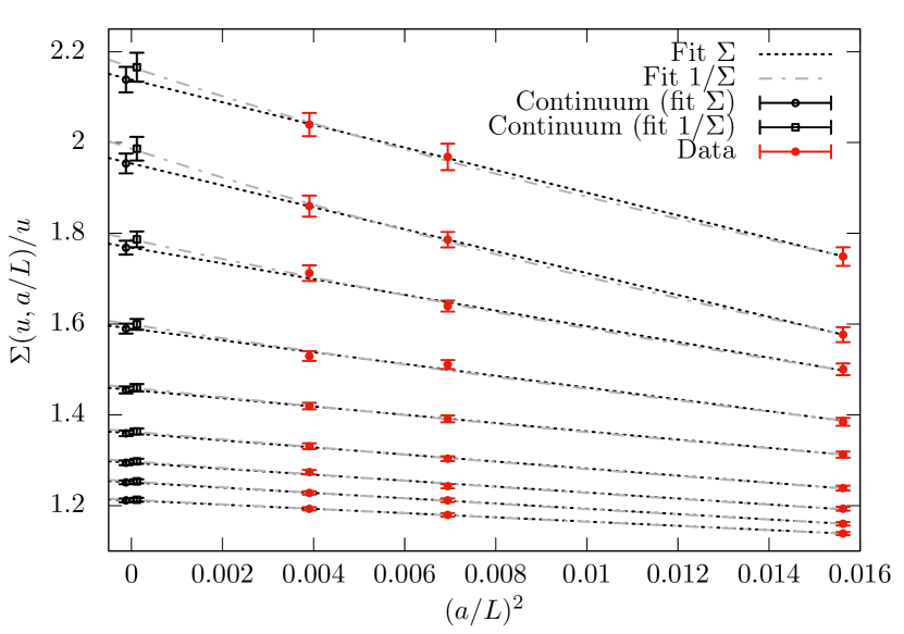
(a) Continuum extrapolation of the step scaling function at the 9 target values of the coupling using as weights for the fit the uncertainty in $\Sigma$. Note that different continuum extrapolations are systematically different.

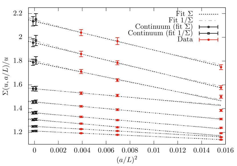
(b) Continuum extrapolation of the step scaling function at the 9 target values of the coupling using as weights for the fit the uncertainty in $\Sigma$ and the systematic estimate of the ${\rm O}(a^{4})$ effects.

Figure 3: Continuum limit of the step scaling function with and without including the systematic effect (28).

We choose to include an estimate of this systematic uncertainty in the weights of our fits.

$$\Delta^{\rm sys}\Sigma_{\rm GF}=0.05\,\Sigma_{\rm GF}\,\bigg{(}8\frac{a}{L}\bigg{)}^{4}\,\frac{u}{u_{\rm max}}\,.$$ (28)

This estimate comes from the size of the $a^{2}$ cutoff effects at our largest value of the coupling (around 20% for our coarser lattice with $L/a=8$), that suggests that the O($a^{4}$) effects are around 5%. This effect is added in quadrature to the uncertainty in $\Sigma_{\rm GF}$. The result of this procedure is apparent if one compares Figures 3(a) and 3(b). The fit functional forms are less constrained by the coarser lattices, resulting in a better agreement between the two extrapolation procedures. The price to pay is an increased error in the extrapolations. All our final numbers follow this fitting procedure. The interested reader can find a detailed discussion in [2].

As stated earlier our non-perturbative data obeys very well the relation $1/\sigma-1/u=\text{constant}$ (the 1-loop functional form). This suggests to fit the continuum step scaling function to a functional form

$$\frac{1}{\sigma_{\rm GF}(v_{i})}-\frac{1}{v_{i}}=Q(v_{i})\,,\qquad Q(u)=\sum_{k=0}^{n_{\rm sig}-1}c_{k}u^{k}\,,$$ (29)

where the number of fit parameters $n_{\rm sig}$ is varied to check the consistency of the results.

Finally one can also combine the continuum extrapolations and the parametrization of the step scaling functions by fitting

$$\frac{1}{\Sigma_{\rm GF}(v_{i},L/a)}-\frac{1}{v_{i}}=Q(v_{i})+\rho(v_{i})(a/L)^{2}\,,\qquad\rho(u)=\sum_{k=0}^{n_{\rho}-1}\rho_{k}u^{k}\,.$$ (30)

We find good fits when $n_{\rho}$ is at least 2. Note that this procedure does not require to shift the data to constant values of the coupling. All these fitting procedures produce a remarkable agreement, as is discussed in detail in [2].

3.3 Determination of the $\beta$-function

Fit	$n_{\rm sig}$	$n_{\rho}$	$u_{1}$	$u_{2}$	$u_{3}$	$u_{4}$	$s(g_{1}^{2},g_{2}^{2})$
$\Sigma$	3	–	$5.870(28)$	$3.954(22)$	$2.976(17)$	$2.385(15)$	$11.00(20)$
$1/\Sigma$	1	3	$5.843(20)$	$3.939(18)$	$2.971(16)$	$2.385(13)$	$10.96(18)$
$1/\Sigma$	2	3	$5.864(26)$	$3.944(19)$	$2.968(16)$	$2.378(14)$	$10.90(18)$
$1/\Sigma$	3	3	$5.864(27)$	$3.944(21)$	$2.968(17)$	$2.378(14)$	$10.90(19)$
(33), $P$	2	2	$5.872(27)$	$3.949(19)$	$2.971(16)$	$2.379(14)$	$10.93(19)$
(33), $P$	3	3	$5.874(28)$	$3.951(22)$	$2.972(17)$	$2.379(14)$	$10.93(20)$

Table 1: Coupling sequence eq. (34) with $u_{0}=11.31$ and scale factors $s(g_{1}^{2},g_{2}^{2})$ for $g_{1}^{2}=2.6723,\,g_{2}^{2}=11.31$ for different fits to cutoff effects and the continuum $\beta$-function. Fits are labeled by $\Sigma$ or $1/\Sigma$ for continuum extrapolations according to eq. (26), eq. (27) or eq. (33). For global fits we specify $n_{\rho}$, while its absence indicates a fit of data extrapolated to the continuum at each value of $u=v_{i}$.

As we have said, our main objective is to compute a ratio of scales, and in order to do this, we need to determine the $\beta$-function. We choose the parametrization

$$\beta(g)=-\frac{g^{3}}{P(g^{2})}\,,\quad P(g^{2})=\sum_{k=0}^{n_{\rm sig}-1}p_{k}g^{2k}\,.$$ (31)

The 1-loop $\beta$-function corresponds to the choice $n_{\rm sig}=1$. The relation between the $\beta$-function and the step scaling function $\sigma_{\rm GF}$

$$\begin{split}\log(2)&=-\int_{\sqrt{u}}^{\sqrt{\sigma(u)}}\frac{{\rm d}x}{\beta(x)}=\int_{\sqrt{u}}^{\sqrt{\sigma(u)}}{\rm d}x\frac{P(x^{2})}{x^{3}}\\ &=-\frac{p_{0}}{2}\left[\frac{1}{\sigma(u)}-\frac{1}{u}\right]+\frac{p_{1}}{2}\log\left[\frac{\sigma(u)}{u}\right]+\sum_{k=1}^{n_{\mathrm{sig}}}\frac{p_{k+1}}{2k}\left[\sigma^{k}(u)-u^{k}\right]\,,\end{split}$$ (32)

is used to fit the coefficients $p_{k}$. An alternative analysis consists in combining the continuum extrapolation with the determination of the $\beta$-function by fitting

$$\log(2)+\widetilde{\rho}(u)(a/L)^{2}=-\int_{\sqrt{u}}^{\sqrt{\Sigma(u,a/L)}}\frac{{\rm d}x}{\beta(x)}\,.$$ (33)

Note that this ansatz provides yet another parametrization of the cutoff effects.

A quantitative test of the agreement between different functional forms consists in analyzing the sequence

$$u_{0}=11.31,\quad u_{i}=\sigma_{\rm GF}^{-1}(u_{i-1})\,,i=1,2,\ldots.$$ (34)

Table 1 contains a sample of the different analysis considered in [2]. The agreement between different ansätze is remarkable. The last column of table 1 is the scale factor

$$s(g_{1}^{2},g_{2}^{2})=\exp\left\{-\int_{g_{1}}^{g_{2}}\frac{dx}{\beta(x)}\right\}\,,$$ (35)

with $g_{1}^{2}=2.6723$ and $g_{2}^{2}=11.31$. As we will see in the next section $\bar{g}^{2}_{\rm GF}(2L_{0})=2.6723(64)$, and therefore this last column is just the result that we are looking for.

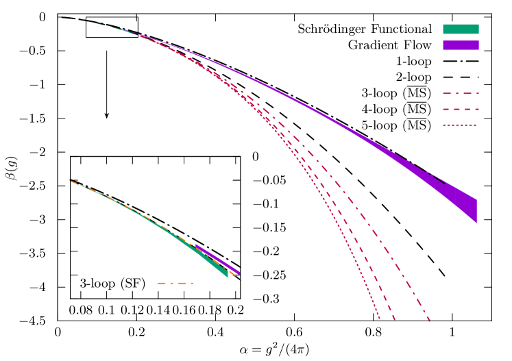
Figure 4: The non-perturbative $\beta$-functions in the SF-scheme from [1] and in the GF-scheme [2]. The plotted 1,2-loop universal part of the perturbative expansion can be compared directly, but higher orders of the perturbative series are unknown for our finite volume GF-scheme. We give an impression of the typical magnitude of higher order perturbative terms in the form of the $\overline{\rm MS}$ scheme, for which we show curves up to 5-loops. On the other hand the 3-loop term is known for the SF scheme.

Figure 4 shows the results of our non-perturbative running both in the SF scheme and in the GF scheme. It is remarkable that the running of the GF coupling follows very closely the 1-loop functional form but with a slightly different coefficient. We conclude that perturbation theory has broken down in most of the range that we cover for $\bar{g}^{2}_{\rm GF}$. The interested reader is invited to read the full discussion in [2].

3.4 The ratio of scales $L_{0}/L_{\rm had}$

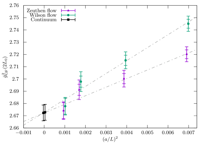
Figure 5: Continuum extrapolation of $\bar{\bar{g}}^{2}_{\rm GF}(2L_{0})$ with the bare parameters determined by the condition $\bar{g}_{\rm SF}^{2}(L_{0})=2.012$. The continuum extrapolation is performed using both the Wilson flow/Clover discretization and our preferred setup Zeuthen flow/LW observable (the latter shows smaller discretization effects). The two types of error bars for each data point correspond to the inclusion or not of the propagated error for the SF coupling, cf. text.

As we have explained the scale $L_{\rm had}$ is defined by the condition $\bar{g}^{2}_{\rm GF}(L_{\rm had})=11.31$. On the other hand the scale $L_{0}$ is defined by $\bar{g}^{2}_{\rm SF}(L_{0})=2.012$. In order to compute the ratio $L_{\rm had}/L_{0}$ using the $\beta$-function determined in the previous section, we need to know the value of the GF coupling at the scale $L_{0}$. To this end we define the function

$$\Phi(u,a/L)=\bar{g}^{2}_{\rm GF}(2L)\Big{|}_{\bar{g}^{2}_{\rm SF}(L)=u,m(L)=0}\,.$$ (36)

The procedure is simple, we tune the bare parameters on several lattices sizes ($L/a=6,8,12,16$) to have $m(L)=0$ and $\bar{g}^{2}_{\rm SF}(L)=2.012$. Note that here we use the Wilson gauge action for the reason explained in section 2. Then we compute the value of the GF coupling at the same values of the bare parameters, but on lattices twice as large. The error in the tuning of the SF coupling is propagated to the GF coupling by using leading order perturbation theory. This procedure has several advantages. On the one hand the SF coupling is computed only on relatively small lattices. This is convenient, since the SF coupling requires large statistics, but its cutoff effects are very small. On the other hand the GF coupling is computed on larger lattices, to avoid large cutoff effects, but with relatively modest statistics one can achieve high statistical precision.

Recall that the SF coupling is defined with a background field, while the boundary conditions of our gradient flow scheme correspond to a zero background field. The connection between the couplings is established via the common bare parameters defined by the condition $\bar{g}^{2}_{\rm SF}(L)=u,m(L)=0$, together with the resolution $a/L$.

Once the estimates of $\Phi(2.012,a/L)$ are determined, we can take the continuum limit and obtain

$$\bar{g}^{2}_{\rm GF}(2L_{0})=\lim_{a/L\rightarrow 0}\Phi(2.012,a/L)=2.6723(64)\,.$$ (37)

Figure 5 shows the continuum extrapolation with two different choices of lattice flow equations.

Given the $\beta$-function determined in the previous section, together with this result, we now obtain (see equation (35))

$$\frac{L_{\rm had}}{L_{0}}=2\times s(2.6723(64),11.31)=21.86(42)\,.$$ (38)

For the value $s(2.6723,11.31)$ we choose the last row of table 1 which has the largest error of all the considered analyses. As indicated, our result for the scale factor also contains the error in $\bar{g}^{2}_{\rm GF}(2L_{0})$ from the matching procedure.

4 Hadronic scales

It is left to fix $L_{\mathrm{had}}$ in physical units from $L_{\mathrm{had}}=(L_{\mathrm{had}}m_{\mathrm{had}})^{(3)}/m_{\mathrm{had}}^{\mathrm{exp}}$ where $m_{\mathrm{had}}$ is an experimentally accessible low energy mass (scale) and $(L_{\mathrm{had}}m_{\mathrm{had}})^{(3)}$ is the dimensionless number computed in QCD with three quark flavors. While it is most natural to use the proton mass, $m_{p}$, it is not that easy to compute it with precision due to large statistical errors in the relevant correlation function at Euclidean times of 1 fm and larger and due to its complicated dependence on the quark masses. Such technical limitations apply similarly to many other quantities. As explained in detail in [42] we are lead to choose the leptonic decay constant of pion and kaon for precision scale setting, even though their phenomenological values $f_{\pi}=130.4(2)\,{\rm MeV}$ and $f_{\rm K}=156.2(7)\,{\rm MeV}$ depend on the knowledge of $V_{\mathrm{ud}}$ and $V_{\mathrm{us}}$ [43].

In fact in order to express $L_{\mathrm{had}}$ in physical units, we first relate $f_{\pi},f_{\rm K}$ to an intermediate large volume scale $t_{0}^{*}$ and then connect that to $L_{\mathrm{had}}$.

4.1 From $\pi$ and K decay constants to the reference scale $t_{0}^{*}$

Our computation of hadronic scales is based on the CLS large volume simulations with two degenerate light quarks, $m_{u}=m_{d}$, and one additional strange quark [3]. In these simulations the trace, $m_{u}+m_{d}+m_{s}$, of the quark mass matrix $M$ is held constant [44] while varying $m_{u}=m_{d}$ in approaching the physical point defined by physical values for $m_{\pi}/f_{\pi\rm K},\,m_{\rm K}/f_{\pi\rm K}$.

Along this trajectory in the quark mass plane the linear combination

$$f_{\pi\rm K}=(2f_{\rm K}+f_{\pi})/3\,$$ (39)

has a particularly simple dependence on the quark masses or equivalently on their hadronic proxies

$$y_{\pi}=\frac{m_{\pi}^{2}}{(4\pi f_{\pi\rm K})^{2}}\,,\quad y_{\mathrm{K}}=\frac{m_{\mathrm{K}}^{2}}{(4\pi f_{\pi\rm K})^{2}}\,.$$ (40)

Namely, in the continuum limit, the expansion around the symmetric point, $y_{\pi}=y_{\mathrm{K}}=y_{\mathrm{sym}}$, reads

$$f_{\pi\rm K}=f_{\pi\rm K}^{\mathrm{symm}}\,[\,(1+h_{2}(y_{\pi}-y_{\mathrm{sym}})^{2}+{\rm O}((y_{\pi}-y_{\mathrm{sym}})^{3})\,]\,.$$ (41)

Furthermore, SU(3) chiral perturbation theory predicts the quark mass dependence [45] free of low energy constants in the form

$$f_{\pi\rm K}=f_{\pi\rm K}^{\mathrm{symm}}\,[\,(1+3L_{\chi}(y_{\mathrm{sym}})-L_{\chi}(y_{\pi})-2L_{\chi}(y_{\mathrm{K}})]+{\rm O}(y^{2})\,.$$ (42)

Here the typical chiral logs

$$L_{\chi}(y)=y\,\log(y)\,,$$ (43)

appear. Both forms eq. (41) and eq. (42) have been used for the extrapolation from the simulation points to the physical point [4]. They agree well within the statistical errors. Still, the small difference at the physical point is used as an estimate of the remaining systematic error in the extrapolation.

Figure 6: Chiral extrapolation of $f_{\pi K}$. In the horizontal axis we plot $\phi_{2}=8t_{0}m_{\pi}^{2}$, and we normalize the data with respect to the symmetric point. The data has been shifted to constant $\phi_{4}=1.11$.

There are more details, e.g. the small cutoff effects have to be taken into account, cf. ref. [4]. There the physical $f_{\pi\rm K}$ was then related to $t_{0}^{*}$, the Gradient Flow scale, $t_{0}$ introduced by M. Lüscher [34] at a particular mass point. This reference mass point is defined in terms of the dimensionless variable

$$\Phi_{4}=8\,t_{0}\,(m_{\rm K}^{2}+\frac{1}{2}m_{\pi}^{2})\,.$$ (44)

We choose the symmetric line and set

$$\left.\Phi_{4}\right|_{m_{\pi}=m_{\pi}^{*}}=1.11\text{\quad for\quad}m_{u}=m_{d}=m_{s}\,,$$ (45)

and

$$t_{0}^{*}=1.11/[12(m_{\pi}^{*})^{2}]\,.$$ (46)

Setting the scale with the phenomenological $f_{\pi\rm K}$ yielded

$$(8t_{0}^{*})^{1/2}=0.413(5)({2})\,{\rm fm}\,,$$ (47)

where the second error is the systematic error from the extrapolation to the physical point. The scale $t_{0}^{*}$ is a good quantity to connect finite and large volumes and it is likely also a good one for other purposes. Being defined in the mass-degenerate theory with quark masses significantly heavier than the physical up and down quark masses, there are only two parameters and, since $m_{\pi}$ is around $400\,{\rm MeV}$, simulations are easy and finite size effects are relatively small.

$\beta$	$am_{\rm q}$	$\tilde{\beta}$	$t_{0}^{*}/a^{2}$	$L_{\rm had}/a$	$({t_{0}^{*}})^{-1/2}L_{\rm had}$
3.4000	0.0068	3.3985	2.862( 5)	12.05(8)	7.13(5)
3.4600	0.0059	3.4587	3.662( 12)	13.51(6)	7.06(3)
3.5500	0.0048	3.5490	5.166( 15)	15.94(6)	7.01(3)
3.5503	0	3.5503		16
3.7000	0.0037	3.6992	8.596( 27)	20.70(9)	7.06(3)
3.7934	0	3.7934		24
3.8500	0.0029	3.8494	13.880(220)	26.42(9)	7.11(8)
3.9753	0	3.9753		32

These properties enable determinations of $t_{0}^{*}/a^{2}$ and $L_{\mathrm{had}}/a$ in a large common range of lattice spacings $a$ and a subsequent controlled continuum extrapolation. We now describe this step in some detail.

4.2 Three flavor $\Lambda$-parameter in physical units

The large volume quantity $t_{0}^{*}$ is defined with finite (degenerate) quark masses. In order to have ${\rm O}(a)$ improvement in its connection to the massless theory, we need to combine $t_{0}^{*}/a^{2}$ and $L_{\rm had}/a$ at matching improved bare coupling [46, 47],

$$\tilde{\beta} = \beta_{\mathrm{CLS}}\,/\,(\,1+\,a\,\hbox{tr}\,M\,b_{g}^{(1)}\,2/\beta_{\mathrm{CLS}})\,+\,{\rm O}(1/\beta_{\mathrm{CLS}})\,,$$ (49)

$$\,\hbox{tr}\,M=3m_{\rm q}\,,\quad b_{g}^{(1)}=0.03600\,.$$

For the evaluation of the bare subtracted quark mass, $am_{\rm q}=1/(2\kappa)-1/(2\kappa_{\rm crit}))$, we need the critical hopping parameter, $\kappa_{\rm crit}$. We estimate it by linear extrapolation in $(a/L)^{3}$ of the critical hopping parameters defined and determined by setting the PCAC mass on $(L/a)^{4}$ lattices to zero. This large $L$ extrapolation is carried out from the $\kappa_{\rm crit}$ for the two largest available lattices, namely $L/a=12,16$ [26]. The relevant numbers are listed in table 4.1. Since the quark masses are small, the ${\rm O}(a)$ correction in eq. (49) is not very significant and it does not matter that we know $b_{g}$ only to 1-loop. It also does not matter whether we extrapolate $\kappa_{\rm crit}$ in $(a/L)^{3}$ or just use the largest lattice. Next we need $L_{\rm had}/a$ at matching bare couplings $\tilde{\beta}$. It is found by interpolating $\tilde{\beta}=\beta$ such that $\bar{g}_{\mathrm{GF}}^{2}=11.31$ for fixed $L_{\rm had}/a$. Details are referred to Astropart. Phys. s:interpol (.) The result is pairs $(L_{\rm had}/a,\beta)$. These are subsequently interpolated as $\log(L_{\rm had}/a)=P(\beta)$. A linear function $P(\beta)$ does not work well, but second and third order polynomials in $\beta$ do and are hardly distinguishable. We use the second order one and take as uncertainty the typical statistical error and the difference of the two polynomials added in quadrature. Table 4.1 contains the results of the first step, at integer values of $L_{\rm had}/a$ as well as the numbers interpolated to the CLS bare couplings $\tilde{\beta}$. The combination $({t_{0}^{*}})^{-1/2}L_{\rm had}$ is listed in the last column of the table. Its continuum extrapolation,

$$({t_{0}^{*}})^{-1/2}L_{\rm had}=\left[({t_{0}^{*}})^{-1/2}L_{\rm had}\right]_{\mathrm{cont}}+B\,\frac{a^{2}}{t_{0}^{*}}\,,$$ (50)

shown in figure 7, is performed with 4,3 and 2 points. The preliminary data point at lattice spacing $a=0.04$ fm is not included in any of these fits but rather shown in the graph to illustrate what we will have shortly. We take the 3-point extrapolation as our central result but enlarge its error of $0.05$ by about a factor four to

$$\left[({t_{0}^{*}})^{-1/2}L_{\rm had}\right]_{\mathrm{cont}}=7.01(18)\,,$$ (51)

such that it covers the largest 1-sigma excursion of all fits, which happens to be the 2-point extrapolation. It is worth mentioning that the $a=0.04$ fm lattice, as well as all others, is simulated with open boundary conditions in time, avoiding the freezing of topology [48]. This will allow very firm conclusions on the continuum limit and a significant reduction of its error. With the previous numbers we find

$$L_{\rm had}=1.03(3)\,{\rm fm}\,,\quad\Lambda_{\rm\overline{MS\kern-0.35002pt}\kern 0.35002pt}^{(3)}=332(14)\,{\rm MeV}\,.$$ (52)

It is likely that the error of $L_{\rm had}$ will shrink significantly once all preliminary steps are replaced by the final ones.

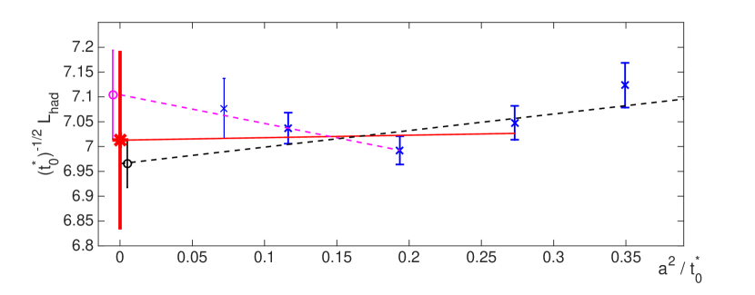
Figure 7: Preliminary continuum extrapolation of $({t_{0}^{*}})^{-1/2}L_{\rm had}$. The large volume simulation with the smallest lattice spacing is unfinished and the correction to shift it to the $\Phi_{4}=1.11$ point has not yet been included. It is only shown to illustrate where we are heading to. Extrapolations with 4,3 and 2 data points are shown together with a range for the continuum value covering all of them, see the text.

5 Connection to the 5-flavor theory and $\alpha_{\rm\overline{MS\kern-0.35002pt}\kern 0.35002pt}(m_{Z})$

There is little doubt that 3-flavor QCD describes the low energy ($E$) phenomena including $L_{\mathrm{had}}f_{\pi\rm K}$ with high precision [49, 43]. In other words, the $(E/m_{c})^{2}$ corrections in the effective theory expansion are small. However, $\Lambda^{(3)}$ needs to be related to $\Lambda^{(5)}$ because physical processes at high energies need $N_{\mathrm{f}}\geq 5$-flavor QCD and the standard $\alpha_{\rm\overline{MS\kern-0.35002pt}\kern 0.35002pt}(m_{Z})$ is defined in the $N_{\mathrm{f}}=5$ theory. It has long been known how to connect these theories perturbatively [50, 9] and we now have 4-loop precision [10, 51] in the relation

$$\bar{g}^{(N_{\mathrm{f}}-1)}(m_{*})=\bar{g}^{(N_{\mathrm{f}})}(m_{*})(1+{\rm O}([\bar{g}^{(N_{\mathrm{f}})}(m_{*})]^{4})\,,$$ (53)

where $m_{*}=\kern 1.0pt\overline{\kern-1.0ptm\kern-1.0pt}\kern 1.0pt_{\rm\overline{MS\kern-0.35002pt}\kern 0.35002pt}(m_{*})$ is the mass of the decoupled quark in the $N_{\mathrm{f}}$-flavor theory and in the ${\rm\overline{MS\kern-0.50003pt}\kern 0.50003pt}$-scheme. Together with

$$\Lambda_{s} = \varphi_{s}(\bar{g}_{s}(\mu))\,\times\,\mu\,,$$ (54)

$$\varphi_{s}(\bar{g}_{s}) = (b_{0}\bar{g}_{s}^{2})^{-b_{1}/(2b_{0}^{2})}{\rm e}^{-1/(2b_{0}\bar{g}_{s}^{2})}\,\times\,\exp\bigg{\{}-\int\limits_{0}^{\bar{g}_{s}}{\rm d}x\ \Big{[}\frac{1}{\beta_{s}(x)}+\frac{1}{b_{0}x^{3}}-\frac{b_{1}}{b_{0}^{2}x}\Big{]}\bigg{\}}\,.$$

$\beta\to\beta^{\mathrm{pert}}_{\rm\overline{MS\kern-0.35002pt}\kern 0.35002pt}$, we can compute the ratio of the $\Lambda$-parameters at given values of $m_{\star}$. The b- and c-quark masses, $m_{\star}=4.18\,{\rm GeV}$ and $m_{\star}=1.275\,{\rm GeV}$ are taken from the PDG [52]. With the available perturbative precision [23, 24, 53, 54, 10, 51], we find

$$\Lambda_{\rm\overline{MS\kern-0.35002pt}\kern 0.35002pt}^{(4)} = 289(14)\,{\rm MeV}\,,\;\;\Lambda_{\rm\overline{MS\kern-0.35002pt}\kern 0.35002pt}^{(5)}=207(11)\,{\rm MeV}\,,\;$$ (55)

$$\alpha_{\rm\overline{MS\kern-0.35002pt}\kern 0.35002pt}(m_{Z}) = 0.1179(10)(2)\,.$$ (56)

The first error in $\alpha$ is just propagated from the one in $\Lambda_{\rm\overline{MS\kern-0.35002pt}\kern 0.35002pt}$, which in turn is obtained by standard error propagation of all previously discussed numbers which were put together. The second error represents our estimate of the uncertainty from using PT in the connection $\Lambda_{\rm\overline{MS\kern-0.35002pt}\kern 0.35002pt}^{(3)}\to\Lambda_{\rm\overline{MS\kern-0.35002pt}\kern 0.35002pt}^{(5)}$. We arrive at it as follows. The $2,3,4$-loop terms in eq. (53) combined with the $3,4,5$-loop running lead to contributions $109,\,15,\,7$ (in units of $10^{-5}$) to $\alpha_{\rm\overline{MS\kern-0.35002pt}\kern 0.35002pt}(m_{Z})$. We take the sum of the last two contributions as our error in eq. (56). Within PT, this represents a very conservative error estimate: the known terms of the series behave similar to a convergent series but we treat it like an asymptotic one. However, we have to stress that we are here using perturbation theory at the scale of the charm quark mass. In principle it is possible that PT is entirely misleading when we apply it at such low scales, decoupling the charm quark. One may note that almost all lattice determinations as well as a number of continuum ones have this same error, but this does not help much. As long as we do not have a computation of all the above steps with $N_{\mathrm{f}}=4$, we have to live with our estimate in eq. (56) and with this – in our opinion unlikely [49] – possibility. It would mean that the second error estimate is far off due to a breakdown of PT for $\Lambda^{(3)}/\Lambda^{(4)}$.

Acknowledgments

This work was done as part of the ALPHA collaboration research programme. We thank our colleagues in the ALPHA collaboration, in particular C. Pena and U. Wolff for many useful discussions. This project has benefited from the joint production of gauge field ensembles with a project computing the running of quark masses. We thank I. Campos, C. Pena and D. Preti for this collaboration. We also thank Pol Vilaseca who computed the used one-loop coefficient $\tilde{c}_{\rm t}$. We thank the computer centres at HLRN (bep00040) and NIC at DESY, Zeuthen for providing computing resources and support. We are indebted to Isabel Campos and thank her and the staff at the University of Cantabria at IFCA in the Altamira HPC facility for computer resources and technical support. S. Sint gratefully acknowledges support by SFI under grant 11/RFP/PHY3218. P.F. acknowledges financial support from the Spanish MINECO’s “Centro de Excelencia Severo Ochoa” Programme under grant SEV-2012-0249, as well as from the MCINN grant FPA2012-31686. M.D.B. thanks the Theoretical Physics Department at CERN for the hospitality and support.

Appendix A Interpolations to $\bar{g}_{\mathrm{GF}}^{2}=11.31$

The point of reference where we match between the hadronic world and the finite volume GF coupling is

$$\bar{g}_{\rm GF}^{2}(L_{\rm had})=11.31\,,\quad m(L_{\rm had})=0\,.$$ (57)

We discuss the present, preliminary, interpolations of the available coupling data to this point separately in this appendix because it is rather technical and the technical difficulties mostly are due to the presently incomplete set of simulation data. This will change soon. The difficulty is that one needs to have the quark mass set to zero in a precisely defined way, with a fixed condition as one varies the lattice spacing. We need a unique line of constant physics. Then cutoff effects are smooth functions of $a$ with the asymptotic form of eq. (50). Eq. (57) is the natural condition, where $m$ is the improved PCAC mass in a $L^{4}$ lattice with the same Dirichlet boundary conditions as in the definition of $\bar{g}_{\rm GF}$. More details are found in [2, 26]. Unfortunately, the presently available data for $\bar{g}_{\rm GF}^{2}=F(L/a,\beta)$ do not homogeneously satisfy $m(L)=0$. For $L/a=12$ they do. But on the larger lattices, $L/a=16,24,32$, we have $m(L/2)=0$, because they originate from the computation of step scaling functions [2]. There is a ${\rm O}((a/L)^{2})$ cutoff effect between the two definitions. We checked for its size: we interpolated the data with $L/a=16$, $m(L/2)=0$ in $\beta$ to $\bar{g}_{\rm GF}^{2}=11.31$ finding $\beta=3.5607$. At this $\beta$, a computation adjusted such that $m(L)=0$ yields $\bar{g}_{\rm GF}^{2}=11.03(6)=11.31-\Delta g^{2}$. Presently, we take this effect into account by treating it as small and in lowest order: we modify eq. (57) for $L/a\geq 16$ to $\bar{g}_{\rm GF}^{2}(L_{\rm had})=11.31+\Delta g^{2}\frac{16^{2}}{(L/a)^{2}}$ at $m(L_{\rm had}/2)=0$. The $L/a,\beta$ points satisfying this condition are found by a quadratic interpolation of the form $F(L/a,\beta)=[k_{0}+k_{1}\beta+k_{2}\beta^{2}]^{-1}$ for fixed $L/a$ implemented by a fit to about 5 data points in the vicinity. The resulting pairs $(L_{\rm had}/a,\beta)=(L_{\rm had}/a,\tilde{\beta})$ are listed in table 4.1.

References

- [1] M. Dalla Brida, P. Fritzsch, T. Korzec, A. Ramos, S. Sint and R. Sommer, Determination of the QCD -parameter and the accuracy of perturbation theory at high energies, Phys. Rev. Lett. 117 (2016) 182001, [1604.06193].
- [2] ALPHA collaboration, M. Dalla Brida, P. Fritzsch, T. Korzec, A. Ramos, S. Sint and R. Sommer, Slow running of the Gradient Flow coupling from 200 MeV to 4 GeV in QCD, (2016) , [1607.06423].
- [3] M. Bruno et al., Simulation of QCD with flavors of non-perturbatively improved Wilson fermions, JHEP 02 (2015) 043, [1411.3982].
- [4] M. Bruno, T. Korzec and S. Schaefer, Setting the scale for the CLS flavor ensembles, (2016) , [1608.08900].
- [5] P. Fritzsch, M. Dalla Brida, T. Korzec, A. Ramos, S. Sint and R. Sommer, Towards a new determination of the QCD Lambda parameter from running couplings in the three-flavour theory, PoS LATTICE2014 (2014) 291, [1411.7648].
- [6] M. Dalla Brida, P. Fritzsch, T. Korzec, A. Ramos, S. Sint and R. Sommer, A status update on the determination of by the ALPHA collaboration, in Proceedings, 33rd International Symposium on Lattice Field Theory (Lattice 2015), 2015. 1511.05831.
- [7] M. Lüscher, Advanced lattice QCD, in Probing the standard model of particle interactions. Proceedings, Summer School in Theoretical Physics, NATO Advanced Study Institute, 68th session, Les Houches, France, July 28-September 5, 1997. Pt. 1, 2, pp. 229–280, 1998. hep-lat/9802029.
- [8] R. Sommer, Non-perturbative QCD: Renormalization, O(a)-improvement and matching to Heavy Quark Effective Theory, in Workshop on Perspectives in Lattice QCD Nara, Japan, October 31-November 11, 2005, 2006. hep-lat/0611020.
- [9] W. Bernreuther and W. Wetzel, Decoupling of Heavy Quarks in the Minimal Subtraction Scheme, Nucl. Phys. B197 (1982) 228–236.
- [10] K. G. Chetyrkin, J. H. Kühn and C. Sturm, QCD decoupling at four loops, Nucl. Phys. B744 (2006) 121–135, [hep-ph/0512060].
- [11] M. Dalla Brida, T. Korzec, S. Sint and P. Vilaseca, High precision renormalization of the non-singlet axial current in lattice QCD with Wilson quarks, in preparation .
- [12] M. Dalla Brida, S. Sint and P. Vilaseca, The chirally rotated Schrödinger functional: theoretical expectations and perturbative tests, JHEP 08 (2016) 102, [1603.00046].
- [13] M. Dalla Brida, P. Fritzsch, T. Korzec, A. Ramos, S. Sint and R. Sommer. in preparation.
- [14] M. Bruno, M. Dalla Brida, P. Fritzsch, T. Korzec, A. Ramos, S. Schaefer et al., The determination of by the ALPHA collaboration, in 6th Workshop on Theory, Phenomenology and Experiments in Flavour Physics: Interplay of Flavour Physics with electroweak symmetry breaking (Capri 2016) Anacapri, Capri, Italy, June 11, 2016, 2016. 1611.05750.
- [15] M. Lüscher, R. Narayanan, P. Weisz and U. Wolff, The Schrödinger functional: a renormalizable probe for non-Abelian gauge theories, Nucl. Phys. B384 (1992) 168–228, [hep-lat/9207009].
- [16] S. Sint, On the Schrödinger functional in QCD, Nucl. Phys. B421 (1994) 135–158, [hep-lat/9312079].
- [17] M. Lüscher, R. Sommer, P. Weisz and U. Wolff, A Precise determination of the running coupling in the SU(3) Yang-Mills theory, Nucl. Phys. B413 (1994) 481–502, [hep-lat/9309005].
- [18] S. Sint and P. Vilaseca, Lattice artefacts in the Schrödinger Functional coupling for strongly interacting theories, PoS LATTICE2012 (2012) 031, [1211.0411].
- [19] ALPHA collaboration, A. Bode, P. Weisz and U. Wolff, Two loop computation of the Schrödinger functional in lattice QCD, Nucl. Phys. B576 (2000) 517–539, [hep-lat/9911018].
- [20] M. Lüscher and P. Weisz, Two loop relation between the bare lattice coupling and the MS coupling in pure SU(N) gauge theories, Phys. Lett. B349 (1995) 165–169, [hep-lat/9502001].
- [21] C. Christou, H. Panagopoulos, A. Feo and E. Vicari, The two loop relation between the bare lattice coupling and the MS-bar coupling in QCD with Wilson fermions, Phys. Lett. B426 (1998) 121–124.
- [22] C. Christou, A. Feo, H. Panagopoulos and E. Vicari, The three loop -function of lattice gauge theories with Wilson fermions, Nucl. Phys. B525 (1998) 387–400, [hep-lat/9801007].
- [23] T. van Ritbergen, J. A. M. Vermaseren and S. A. Larin, The four loop beta function in quantum chromodynamics, Phys. Lett. B400 (1997) 379–384, [hep-ph/9701390].
- [24] M. Czakon, The Four-loop QCD beta-function and anomalous dimensions, Nucl.Phys. B710 (2005) 485–498, [hep-ph/0411261].
- [25] JLQCD, CP-PACS collaboration, N. Yamada et al., Non-perturbative O(a)-improvement of Wilson quark action in three-flavor QCD with plaquette gauge action, Phys.Rev. D71 (2005) 054505, [hep-lat/0406028].
- [26] P. Fritzsch and T. Korzec, Simulating the QCD Schrödinger Functional with three massless quark flavors, in preparation (2016) .
- [27] M. Lüscher and S. Schaefer, Lattice QCD with open boundary conditions and twisted-mass reweighting, Comput. Phys. Commun. 184 (2013) 519–528, [1206.2809].
- [28] PACS-CS collaboration, S. Aoki et al., Precise determination of the strong coupling constant in lattice QCD with the Schrödinger functional scheme, JHEP 0910 (2009) 053, [0906.3906].
- [29] M. Lüscher and P. Weisz, O(a) improvement of the axial current in lattice QCD to one loop order of perturbation theory, Nucl. Phys. B479 (1996) 429–458, [hep-lat/9606016].
- [30] ALPHA collaboration, G. de Divitiis, R. Frezzotti, M. Guagnelli, M. Lüscher, R. Petronzio, R. Sommer et al., Universality and the approach to the continuum limit in lattice gauge theory, Nucl. Phys. B437 (1995) 447–470, [hep-lat/9411017].
- [31] A. Ramos, The Yang-Mills gradient flow and renormalization, PoS LATTICE2014 (2015) 017, [1506.00118].
- [32] P. Fritzsch and A. Ramos, The gradient flow coupling in the Schrödinger Functional, JHEP 10 (2013) 008, [1301.4388].
- [33] R. Narayanan and H. Neuberger, Infinite N phase transitions in continuum Wilson loop operators, JHEP 0603 (2006) 064, [hep-th/0601210].
- [34] M. Lüscher, Properties and uses of the Wilson flow in lattice QCD, JHEP 1008 (2010) 071, [1006.4518].
- [35] M. Lüscher and P. Weisz, Perturbative analysis of the gradient flow in non-abelian gauge theories, JHEP 1102 (2011) 051, [1101.0963].
- [36] L. Del Debbio, G. M. Manca and E. Vicari, Critical slowing down of topological modes, Phys. Lett. B594 (2004) 315, [hep-lat/0403001].
- [37] P. Fritzsch, A. Ramos and F. Stollenwerk, Critical slowing down and the gradient flow coupling in the Schrödinger functional, PoS Lattice2013 (2013) 461, [1311.7304].
- [38] S. Aoki, R. Frezzotti and P. Weisz, Computation of the improvement coefficient to one loop with improved gluon actions, Nucl. Phys. B540 (1999) 501, [hep-lat/9808007].
- [39] S. Takeda, S. Aoki and K. Ide, A Perturbative determination of boundary improvement coefficients for the Schrödinger functional coupling at one loop with improved gauge actions, Phys. Rev. D68 (2003) 014505, [hep-lat/0304013].
- [40] P. Vilaseca, private communication (2015) .
- [41] A. Ramos and S. Sint, Symanzik improvement of the gradient flow in lattice gauge theories, Eur. Phys. J. C76 (2016) 15, [1508.05552].
- [42] R. Sommer, Scale setting in lattice QCD, PoS LATTICE2013 (2014) 015, [1401.3270].
- [43] S. Aoki et al., Review of lattice results concerning low-energy particle physics, (2016) , [1607.00299].
- [44] W. Bietenholz et al., Tuning the strange quark mass in lattice simulations, Phys. Lett. B690 (2010) 436–441, [1003.1114].
- [45] J. Gasser and H. Leutwyler, Chiral Perturbation Theory: Expansions in the Mass of the Strange Quark, Nucl. Phys. B250 (1985) 465–516.
- [46] S. Sint and R. Sommer, The Running coupling from the QCD Schrödinger functional: A One loop analysis, Nucl. Phys. B465 (1996) 71–98, [hep-lat/9508012].
- [47] M. Lüscher, S. Sint, R. Sommer and P. Weisz, Chiral symmetry and O(a) improvement in lattice QCD, Nucl. Phys. B478 (1996) 365–400, [hep-lat/9605038].
- [48] M. Lüscher and S. Schaefer, Lattice QCD without topology barriers, JHEP 1107 (2011) 036, [1105.4749].
- [49] ALPHA collaboration, M. Bruno, J. Finkenrath, F. Knechtli, B. Leder and R. Sommer, Effects of Heavy Sea Quarks at Low Energies, Phys. Rev. Lett. 114 (2015) 102001, [1410.8374].
- [50] S. Weinberg, Effective gauge theories, Phys.Lett. B91 (1980) 51.
- [51] Y. Schröder and M. Steinhauser, Four-loop decoupling relations for the strong coupling, JHEP 01 (2006) 051, [hep-ph/0512058].
- [52] Particle Data Group collaboration, K. A. Olive et al., Review of Particle Physics, Chin. Phys. C38 (2014) 090001.
- [53] P. A. Baikov, K. G. Chetyrkin and J. H. Kühn, Five-Loop Running of the QCD coupling constant, (2016) , [1606.08659].
- [54] T. Luthe, A. Maier, P. Marquard and Y. Schröder, Towards the five-loop Beta function for a general gauge group, JHEP 07 (2016) 127, [1606.08662].