Model Spaces of Regularity Structures
for Space-Fractional SPDEs

Abstract

We study model spaces, in the sense of Hairer, for stochastic partial differential equations involving the fractional Laplacian. We prove that the fractional Laplacian is a singular kernel suitable to apply the theory of regularity structures. Our main contribution is to study the dependence of the model space for a regularity structure on the three-parameter problem involving the spatial dimension, the polynomial order of the nonlinearity, and the exponent of the fractional Laplacian. The goal is to investigate the growth of the model space under parameter variation. In particular, we prove several results in the approaching subcriticality limit leading to universal growth exponents of the regularity structure. A key role is played by the viewpoint that model spaces can be identified with families of rooted trees. Our proofs are based upon a geometrical construction similar to Newton polygons for classical Taylor series and various combinatorial arguments. We also present several explicit examples listing all elements with negative homogeneity by implementing a new symbolic software package to work with regularity structures. We use this package to illustrate our analytical results and to obtain new conjectures regarding coarse-grained network measures for model spaces.

Submitted version

2010 Mathematical Subject Classification. 60H15, 35R11 (primary), 05C05, 82B20 (secondary).

Keywords and phrases. Stochastic partial differential equations, regularity structures, fractional Laplacian, nonhomeomorphic rooted trees, subcriticality boundary.

1 Introduction

Our main starting point in this work are stochastic partial differential equations (SPDEs) of the form

$$\partial_{t}u=\Delta^{\rho/2}u+f(u)+\xi\;,\qquad\partial_{t}:=\frac{\partial}{\partial t}\;,$$ (1.1)

where $\Delta^{\rho/2}:=-(-\Delta)^{\rho/2}$ is the fractional Laplacian for $\rho\in(0,2]$, $f$ is a polynomial defined in (1.2), $\xi=\xi(t,x)$ is the noise (which we shall often take as space-time white noise as discussed below), $u=u(t,x)$ and $(t,x)\in[0,+\infty)\times\mathbb{T}^{d}$, where $\mathbb{T}^{d}$ is the unit torus in $\mathbb{R}^{d}$ so that we work with periodic boundary conditions. We also write $f$ explicitly as

$$f(u):=\sum_{j=0}^{N}a_{j}u^{j}\;,$$ (1.2)

where the degree $N$ will be restricted, depending upon the dimension $d$. The technical development of this paper starts in Section 2. Here we outline the origins of the questions of this work and provide a formal overview of our results.

There are several motivations to study (1.1). First of all, the case $\alpha=2$, corresponding to the classical Laplacian, has been studied in great detail for the deterministic system ($\xi\equiv 0$), under various names for different polynomial nonlinearities such as the Allen–Cahn equation [2], the Nagumo equation [34], the Fisher–Kolmogorov–Petrowski–Piscounov equation [15, 30], the Ginzburg–Landau equation [12] or as normal forms (or modulation/amplitude equations) for bifurcations of PDEs [26]. Recently, there has been considerable interest to extend the scope to either the stochastic case ($\xi\not\equiv 0$) or to include other differentiable operators, such as the fractional Laplacian, which is a nonlocal operator; see [11, 1] or Section 3 for one precise definition of the fractional Laplacian. Hence, it is a natural theoretical question, how stochastic terms and nonlocal operators can be combined. For very rough stochastic driving terms $\xi$ already existence and regularity questions for (1.1) are nontrivial. Indeed, pursuing the classical route to re-write (1.1) in a mild formulation [37] using the semigroup $t\mapsto\smash{{\textnormal{e}}^{t\Delta^{\rho/2}}}$ can lead to a fixed-point problem, where the products in the polynomial (1.2) are not well-defined as $u$ may only have the regularity of a generalized function (or distribution). This issue not only appears for the classical stochastic Allen–Cahn equation ($\alpha=2$, $\xi$ space-time white noise, $d\in\{2,3\}$, $N=3$) but also in many other SPDEs such as the Kardar–Parisi–Zhang equation [28, 21], the $\Phi^{4}_{3}$-model [24], and several other SPDEs. To overcome this problem for different classes of SPDEs, Martin Hairer developed a unified theory of regularity structures in combination with a renormalization scheme [22]. The basic idea is to consider an abstract algebraic structure, the regularity structure, in which we may solve a suitable fixed-point problem. Furthermore, this solution procedure is compatible with taking limits of a smoothed version of the original problem and reconstructing a “physical” solution from objects in the regularity structure [22]. A key ingredient of the fixed-point argument is that under a parabolic space-time scaling, the heat semigroup associated to the classical Laplacian is regularizing of order two, i.e., we essentially gain two derivatives after a convolution of a function/distribution with the heat kernel. This smoothing effect compensates the rough driving by $\xi$ for certain, so-called subcritical, nonlinearities. A related theory achieving the definition of low-regularity products of functions uses paracontrolled distributions [27, 18], developed by Gubinelli and co-authors, and has also been applied to several classes of SPDEs [20, 19]. Also in this theory, one makes use of the smoothing properties of differential operators in the SPDE.

Remark 1.1.

In this paper, we focus on the theory of regularity structures. However, since we study a space of functions, the space of modelled distributions, which can be used to expand the solution of the SPDE (1.1) as a series, it is expected that our results could be re-interpreted in the context of paracontrolled calculus in future work. ∎

From the theory of fractional differential Laplace operators, or more generally Riesz–Feller operators, and associated ideas developed in the context of Lévy processes and anomalous diffusion, it is known that the fractional Laplacian has less smoothing properties than the classical Laplacian. Hence, it is natural to ask, how this restricts the class of SPDEs tractable via regularity structures.

A second key motivation to study (1.1) arose out of recent work [5] by the authors of this paper, where the key object of study was the FitzHugh–Nagumo SPDE

$$\partial_{t}u =\Delta u+u(1-u)(u-p)-v+\xi\;,$$

$$\partial_{t}v =g(u,v)\;,$$ (1.3)

where $p\in[0,\frac{1}{2}]$ is a parameter and $g(u,v):\mathbb{R}\times\mathbb{R}^{m}\rightarrow\mathbb{R}^{m}$ is linear. The main problems to apply the theory of regularity structures to (1.3) are to deal with multiple components and especially the missing spatial regularization properties as the $v$-components do not contain a spatial differential operator. In [5], this problem is overcome by introducing a spatially non-smoothing operator for the $v$-components and then working through the required Schauder estimates for this operator again by modifying the relevant parts of [22]. One may argue that it could be more convenient to try to follow the classical strategy developed for hyperbolic conservation laws [13] and introduce a viscous regularization

$$\partial_{t}u =\Delta u+u(1-u)(u-p)-v+\xi\;,$$

$$\partial_{t}v =\delta_{v}\Delta v+g(u,v)\;,$$ (1.4)

prove existence and regularity for (1.4) and then consider the limit $\delta_{v}\rightarrow 0$. Albeit appealing, this approach does not seem to work well in combination with regularity structures as $\delta_{v}\Delta$ is a regularizing operator of order two for any $\delta_{v}>0$ but has no spatial regularization properties for $\delta_{v}=0$. Hence, one idea is to replace $\delta_{v}\Delta$ by $\Delta^{\rho/2}$ and consider the limit $\rho\rightarrow 0$ instead. This strategy seems more suited to work with regularity structures but we are still lacking a full understanding of one-component reaction–diffusion SPDEs with polynomial nonlinearities and involving the fractional Laplacian. This paper provides the first steps to fill this gap.

Additional motivation arises from the theory of regularity structures itself. The theory does require certain nonlocal operators, even when working with the classical Laplacian, so working with general nonlocal operators seems natural and could lead to a better understanding of regularity structures. Furthermore, the algebraic results on regularity structures recently announced in [23], developed simultaneously to the present work and available as first versions in [8, 9], are also relevant as one may ask, how the viewpoint of rooted trees as regularity structure elements may be exploited further. We remark that we are going to study a problem, where the exponent of the fractional Laplacian $\rho$ allows us to approach the border between subcritical SPDEs with finite renormalization group (i.e. super-renormalizable SPDEs) [21] and infinite-dimensional renormalization groups.

From the perspective of dynamical aspects of the SPDEs (1.1) and (1.3), it is known that solution properties can change considerably if external noise is added [3, 17] or standard diffusion is replaced by a jump process [29, 33]. Hence, combining and comparing these two aspects is definitely going to lead to new applications.

In this paper, we focus on the parametric problem for building the regularity structure, i.e., we only study the model space of the structure, not yet the renormalization procedure, which might simplify anyhow due to the very recent results in [23, 8, 9]; however, a detailed renormalization study of (1.1) is still expected to reveal interesting effects, e.g., in the context of large deviations [25, 4]. There are three key parameters for (1.1), whose influence we would like to study:

• the spatial dimension $d\in\mathbb{N}$,

• the polynomial degree $N\in\mathbb{N}$,

• the fractional exponent $\rho\in(0,2]$,

where the choice of interval for $\rho$ is motivated by the regularization of the FitzHugh–Nagumo problem as well as the representative horizontal cut through the Feller–Takayasu diamond [29]; in particular, our results also hold for Riesz–Feller operators with asymmetry parameter $\theta$ and $|\theta|\mathrel{\leqsymb}\min\{\alpha,2-\alpha\}$ but we do not spell the results out to simplify the notation. There seems currently to be no detailed study available covering the parametric dependence of regularity structures, so we hope that giving this dependence more explicitly for a key example such as (1.1) helps to solidify the general understanding of regularity structures. The main results of our work can be summarized in a non-technical form as follows:

1. We verify that the fractional Laplacian falls within the class of singular integral operators considered by Hairer. We determine for which parameter values the SPDE (1.1) fulfils the local subcriticality condition, which is necessary for the application of regularity structures to construct solutions; the main condition for space-time white noise is

   $$\rho>\rho_{c}=d\frac{N-1}{N+1}\;;$$

   see Section 3 and Theorem 4.3.

2. We study the model space ${\mathcal{T}}_{F}$ and its dependence on the three parameters $N,d,\rho$ analytically. There are several interesting results for space-time white-noise:

   • We relate the number of negative homogeneities to solutions of constrained Diophantine equations for rational $\rho$; see Proposition 4.8.

   • We prove that the number of negative homogeneities in the index set diverges like $(\rho-\rho_{\rm{c}})^{-1}$ as $\rho$ approaches the subcriticality limit from above; see Theorem 4.12.

   • We prove that the number of negative-homogeneous elements of the model space diverges in the subcriticality limit like $(\rho-\rho_{\rm{c}})^{3/2}\exp(\beta_{N}d(\rho-\rho_{\rm{c}})^{-1})$ as $\rho\searrow\rho_{c}$ with an explicitly computable constant $\beta_{N}$; see Theorem 4.18 and Theorem 4.20.

   • We determine statistical properties of the negative-homogeneous elements of the model space viewed as rooted trees, such as the asymptotic relative degree distribution (Proposition 5.4) and the homogeneity distribution (Proposition 5.3). In particular, we show that all trees are obtained by pruning a regular tree of degree $N+1$ of at most $N-1$ edges.

   For a more general noise, we have the following result:

   • For any value of $(\rho,N,d)$, there exists a choice of noise such that the SPDE (1.1) is subcritical and its model space has elements of homogeneity of $0^{-}$, i.e., $0-\kappa$ for any sufficiently small $\kappa$; see Proposition 4.14.

3. We study numerically the statistical properties of elements in ${\mathcal{T}}_{F}$ viewed as rooted trees using graph-theoretical measures. We implement a symbolic software package to compute with the rooted trees. Based upon computing several benchmark examples, we conjecture a number of statistical limit graph properties. These conjectures include the existence of limits of coarse-grained graph measures as well as the existence of a limiting probability distribution of negative homogeneities formed (for $\rho\in\mathbb{Q}$) similar to a fractal construction; see Section 6.

In summary, the approach towards the theory of regularity structures in this paper is quite different from previous works using the theory. Here we focus on the parametric structure of the model space and SPDEs approaching the subcriticality condition in a parameter limit. This approach is similar to strategies employed in statistical physics to capture “universal” exponents as well as to parameter studies in dynamical systems. This view reveals that there is a lot to be learned just by studying the model space as an object itself.

The paper is structured as follows: In Section 2, we review some basics about regularity structures and fix the notation. In Section 3 we provide the details for the singular kernels, as introduced by Hairer, in the context of the fractional Laplacian. In the main Section 4, we construct the model space ${\mathcal{T}}_{F}$ for (1.1), we determine the subcriticality boundary, and we study the growth of the number of elements in ${\mathcal{T}}_{F}$. In Section 5, we derive several statistical properties of the model space near the subcriticality boundary. In Section 6, we present the computations carried out by the new symbolic computation package.

Notations: If $x\in\mathbb{R}$, then $\lfloor x\rfloor$ denotes the largest integer less than or equal to $x$. We write $|x|$ to denote either the absolute value of $x\in\mathbb{R}$ or the $\ell^{1}$-norm of $x\in\mathbb{R}^{d}$, while $\|x\|$ denotes the Euclidean norm of $x\in\mathbb{R}^{d}$. If $A$ is a finite set, then $|A|$ stands for the cardinality of $A$. We use the notation $\text{supp}(f)$ for the support of a function $f$, and $f\asymp g$ to indicate that $f/g$ is bounded uniformly above and below by strictly positive constants. For the identity mapping on a set or space we write Id.

Acknowledgments: We would like to thank Romain Abraham, Marie Albenque and Kilian Raschel for advice on the combinatorics of trees. CK has been supported by the VolkswagenStiftung via a Lichtenberg Professorship.

2 Regularity Structures

We briefly recall the basic notions from [22] to fix the notation. Furthermore, this section separates out the parts of the theory of regularity structures that are required to consider the fractional SPDE (1.1), i.e., to build the regularity structure associated to (1.1). Let $\mathfrak{T}=({\mathcal{A}},{\mathcal{T}},{\mathcal{G}})$ denote a regularity structure. The index set ${\mathcal{A}}\subset\mathbb{R}$ is locally finite, bounded below and with $0\in{\mathcal{A}}$, the model space ${\mathcal{T}}=\oplus_{\alpha\in{\mathcal{A}}}{\mathcal{T}}_{\alpha}$ is a graded vector space with Banach spaces ${\mathcal{T}}_{\alpha}$, and ${\mathcal{G}}$ is the structure group of linear operators acting on ${\mathcal{T}}$, such that for every $\Gamma\in{\mathcal{G}}$, $\alpha\in{\mathcal{A}}$, $\tau\in{\mathcal{T}}_{\alpha}$ one has

$$\Gamma\tau-\tau\in\bigoplus_{\beta<\alpha}{\mathcal{T}}_{\beta}\;.$$ (2.1)

Roughly speaking, one has to view ${\mathcal{T}}$ as containing abstract symbols representing basic functions or distributions, while ${\mathcal{G}}$ links together different basis points for general abstract expansions of functions or distributions. Two basic examples are the polynomial regularity structure (see Example 2.1 below) and rough paths [16]. It is standard to require that ${\mathcal{T}}_{0}$ is isomorphic to $\mathbb{R}$ with unit vector ${\bf 1}$ as well as $\Gamma{\bf 1}={\bf 1}$ for all $\Gamma\in{\mathcal{G}}$. It will become clear later on that the index $\alpha$ can be associated to “regularity” classes. Given another regularity structure $\widehat{\mathfrak{T}}=(\hat{{\mathcal{A}}},\hat{{\mathcal{T}}},\hat{{\mathcal{G}}})$, one writes ${\mathfrak{T}}\subset\widehat{\mathfrak{T}}$ if ${\mathcal{A}}\subset\hat{{\mathcal{A}}}$, there exists an injective map $\iota:{\mathcal{T}}\rightarrow\hat{{\mathcal{T}}}$ such that $\iota({\mathcal{T}}_{\alpha})\subset\hat{{\mathcal{T}}}_{\alpha}$ for all $\alpha\in{\mathcal{A}}$, $\iota({\mathcal{T}})$ is invariant under $\hat{{\mathcal{G}}}$, and $j$ given via $j(\cdot):=\iota^{-1}(\cdot)\iota$ is a surjective group homomorphism from $\hat{{\mathcal{G}}}$ to ${\mathcal{G}}$. We endow $\mathbb{R}^{d+1}$, using coordinates $z=(t,x)\in\mathbb{R}\times\mathbb{R}^{d}$, with a scaling

$${\mathfrak{s}}:=({\mathfrak{s}}_{0},{\mathfrak{s}}_{1},\ldots,{\mathfrak{s}}_{d})\in\mathbb{N}^{d+1}$$

which induces a scaled degree for each multiindex $k\in\mathbb{N}_{0}^{d+1}$ given by

$$|k|_{\mathfrak{s}}:=\sum_{i=0}^{d}{\mathfrak{s}}_{i}k_{i}$$

and a scaling map

$${\mathcal{S}}_{\mathfrak{s}}^{\delta}:\mathbb{R}^{d+1}\rightarrow\mathbb{R}^{d+1},\qquad{\mathcal{S}}_{\mathfrak{s}}^{\delta}(t,x):=(\delta^{-{\mathfrak{s}}_{0}}t,\delta^{-{\mathfrak{s}}_{1}}x_{1},\ldots,\delta^{-{\mathfrak{s}}_{d}}x_{d})\;,$$

as well as a scaled metric on $\mathbb{R}^{d+1}$ defined as

$$d_{\mathfrak{s}}((t,x),(s,y)):=|t-s|^{1/{\mathfrak{s}}_{0}}+\sum_{i=1}^{d}|x_{i}-y_{i}|^{1/{\mathfrak{s}}_{i}}\;.$$

It is useful to employ the notations $|{\mathfrak{s}}|:=\sum_{i=0}^{d}{\mathfrak{s}}_{i}$ as well as $d_{\mathfrak{s}}((t,x),(s,y))=:\|(t,x)-(s,y)\|_{\mathfrak{s}}$ although $\|\cdot\|_{\mathfrak{s}}$ is not a norm. The associated shifted scalings for a function $\phi$ are defined as

$$\bigl{(}{\mathcal{S}}^{\delta}_{{\mathfrak{s}},\bar{z}}\phi\bigr{)}(z):=\delta^{-|{\mathfrak{s}}|}\phi\bigl{(}{\mathcal{S}}^{\delta}_{\mathfrak{s}}(z-\bar{z})\bigr{)}\;.$$

Essentially, one employs scalings in the theory of regularity structures to bring the action of certain differential operators on a common invariant scale. Here we restrict to the scalings necessary for the operator $\partial_{t}+(-\Delta)^{\rho/2}$, which explains the splitting between the first time coordinate and the spatial coordinates in the scaling.

Example 2.1.

The polynomial regularity structure $(\bar{{\mathcal{A}}},\bar{{\mathcal{T}}},\bar{{\mathcal{G}}})$ on $\mathbb{R}^{d+1}$ associated with the scaling ${\mathfrak{s}}$ is given by $\bar{{\mathcal{A}}}=\mathbb{N}_{0}$, by the polynomial ring $\bar{{\mathcal{T}}}=\mathbb{R}[X_{0},X_{1},\ldots,X_{d}]$ with a grading induced by the scaled degree

$$\bar{{\mathcal{T}}}_{n}:=\textnormal{span}\{X^{k}:|k|_{\mathfrak{s}}=n\}\;,$$

and $\bar{{\mathcal{G}}}$ given by translations. Here we use the multiindex notation $X^{k}=X_{0}^{k_{0}}\dots X_{d}^{k_{d}}$. Indeed, the abstract polynomials have a natural structure group with elements $\Gamma_{h}\in\bar{{\mathcal{G}}}$ acting by $\Gamma_{h}X^{k}=(X+h)^{k}$ for $h\in\mathbb{R}^{d+1}$ so $\bar{{\mathcal{G}}}\simeq\mathbb{R}^{d}$; see [22, Sec 2.2]. The requirement (2.1) then just means for the polynomial regularity structure that translating a polynomial and then subtracting the original one leaves only lower-degree terms. For all regularity structures considered here, we always assume that $\bar{{\mathcal{T}}}\subset{\mathcal{T}}$. ∎

In general, whenever $\tau\in{\mathcal{T}}_{\alpha}$, we declare its homogeneity to be given by $|\tau|_{\mathfrak{s}}=\alpha$. The homogeneity is supposed to reflect a type of Hölder continuity with respect to the scaled metric $d_{\mathfrak{s}}$ of the function or distribution $\tau$ represents. If $\alpha>0$, then a function $f:\mathbb{R}^{d+1}\to\mathbb{R}$ belongs to ${\mathcal{C}}^{\alpha}_{\mathfrak{s}}$ if it satisfies a similar condition on increments as classical Hölder functions, but for the scaled metric (see [22, Def. 2.14] for a precise definition). If $\alpha<0$, then a Schwartz distribution $\xi$ is said to belong to ${\mathcal{C}}^{\alpha}_{\mathfrak{s}}$ if there exists a constant $C$ such that

$$\bigl{|}\langle\xi,{\mathcal{S}}^{\delta}_{{\mathfrak{s}},z}\eta\rangle\bigr{|}\mathrel{\leqsymb}C\delta^{\alpha}$$ (2.2)

for any sufficently smooth test function $\eta$ supported in a $d_{\mathfrak{s}}$-ball of radius $1$ and any $\delta\in(0,1]$ (see [22, Def. 3.7]).

There are two (out of several more) important steps we address in this paper regarding regularity structures for (1.1). Firstly, we have to check whether the fractional Laplacian fits into the framework of singular integral operators required in the theory of regularity structures [22]. Only if this is the case, we have a hope of being able to directly apply the theory. This step is quite straightforward. The second step we cover here is to build the index set ${\mathcal{A}}$ and model space ${\mathcal{T}}$ and study their dependence upon parameters. This step is already substantially more involved.

There are two important further steps in the analysis of the SPDE that we do not consider here, but for which a general method is given in [22, 8, 9]. The first step is the definition and analysis of a fixed-point equation, equivalent to a regularised version of the SPDE, but formulated in a space of modelled distributions ${\mathcal{D}}^{\gamma}$ (an analogue of the Hölder space on the level of the regularity structure, cf. [22, Def. 3.1]). The second step is the renormalisation procedure needed to make sense of the limit of vanishing regularisation. For both steps, a good understanding of the model space is essential. Indeed, we observe the following:

• The negative-homogeneous sector $\bigoplus_{\alpha\in{\mathcal{A}}\cap\mathbb{R}_{-}}{\mathcal{T}}_{\alpha}$ carries the distribution-valued part of the solution. While in the case of the standard Laplacian ($\rho=2$) with space-time white noise, this part only contains the stochastic convolution of heat kernel and noise, for general fractional Laplacians it may contain many more terms.

• The constants needed to renormalise the equation are determined by summing over contractions of subtrees in negative-homogeneous elements, as discussed in [23, 8, 9]. We expect that the number of renormalisation constants diverges as one approaches the subcriticality boundary.

3 Singular Kernels

To formulate fixed-point equations associated to (S)PDEs in the context of regularity structures, we have to consider integration against singular integral kernels. Consider a linear differential operator $L$ with constant coefficients acting on $u=u(t,x)=u(z)$ for $z\in\mathbb{R}^{d+1}$. Let $G=G(t,x)=G(z)$ denote the fundamental solution or kernel, i.e.,

$$(LG)(z)=\bm{\delta}(z)\;,$$

for $t>0$, where $\bm{\delta}\in{\mathcal{S}}(\mathbb{R}^{d+1})$ denotes the delta-distribution. Frequently, $G$ is a singular kernel. Consider for instance the heat operator $L:=\partial_{t}-\sum_{j=1}^{d}\partial_{x_{j}x_{j}}^{2}$ with associated heat kernel

$$G_{2}(z,{\bar{z}})=\frac{1}{|4\pi(t-\bar{t}\,)|^{d/2}}\exp\left(-\frac{\|x-{\bar{x}}\|^{2}}{4(t-\bar{t}\,)}\right)\;.$$

Here ${\bar{z}}=({\bar{t}},{\bar{x}})\in\mathbb{R}^{d+1}$ and the subscript of $G$, fixed here to $2$, is used to distinguish the heat kernel $G_{2}$ from other kernels $G_{\rho}$ we are going to consider below, while the subscript will be omitted for the general theory of singular kernels. Note that $G_{2}$ is singular at $z={\bar{z}}$.

3.1 Hairer’s Singular Kernels

In Hairer’s theory of regularity structures, one first aims to decompose a general kernel $G:\mathbb{R}^{d+1}\times\mathbb{R}^{d+1}\rightarrow\mathbb{R}$ via

$$G(z,{\bar{z}})=K(z,{\bar{z}})+R(z,{\bar{z}})\;,$$

where $K$ is the singular part and $R$ is a smooth part. So the key object is $K$ and we recall the assumptions on $K=K(z,{\bar{z}})$ as stated in [22, Assumption 5.1 / Assumption 5.4]. A mapping $K:\mathbb{R}^{d+1}\times\mathbb{R}^{d+1}\rightarrow\mathbb{R}$ is called a regularizing kernel of order $\beta>0$ if $K$ can be decomposed as

$$K(z,{\bar{z}})=\sum_{n\mathrel{\geqsymb}0}K_{n}(z,{\bar{z}})$$ (3.1)

and for all $n\mathrel{\geqsymb}0$, $\text{supp}(K_{n})\subseteq\{(z,{\bar{z}})\in\mathbb{R}^{d+1}\times\mathbb{R}^{d+1}:\|z-{\bar{z}}\|_{\mathfrak{s}}\mathrel{\leqsymb}2^{-n}\}$, for any $k,l\in\mathbb{N}_{0}^{d+1}$, there exists a constant $C$ such that

$$\bigl{|}{\textnormal{D}}_{1}^{k}{\textnormal{D}}_{2}^{l}K_{n}(z,{\bar{z}})\bigr{|} \mathrel{\leqsymb}C2^{(|{\mathfrak{s}}|-\beta+|l|_{\mathfrak{s}}+|k|_{\mathfrak{s}})n}\;,$$

$$\left|\int_{\mathbb{R}^{d+1}}(z-{\bar{z}})^{l}{\textnormal{D}}_{2}^{k}K_{n}(z,{\bar{z}})~{}{\textnormal{d}}z\right| \mathrel{\leqsymb}C2^{-\beta n}\;,$$

$$\left|\int_{\mathbb{R}^{d+1}}({\bar{z}}-z)^{l}{\textnormal{D}}_{1}^{k}K_{n}(z,{\bar{z}})~{}{\textnormal{d}}{\bar{z}}\right| \mathrel{\leqsymb}C2^{-\beta n}\;,$$ (3.2)

hold uniformly over all $n\mathrel{\geqsymb}0$ and all $z,{\bar{z}}\in\mathbb{R}^{d}$, and there exists $r>0$ such that

$$\int_{\mathbb{R}^{d+1}}K_{n}(z,{\bar{z}})P({\bar{z}})~{}{\textnormal{d}}{\bar{z}}=0$$ (3.3)

for every $n\mathrel{\geqsymb}0$, every $z\in\mathbb{R}^{d}$ and every monomial $P$ of degree $k^{*}\in\mathbb{N}_{0}^{d+1}$ with $|k^{*}|_{\mathfrak{s}}\mathrel{\leqsymb}r$. We also refer to the condition (3.3) as $r$-order annihilation of polynomials.

If $G(z,{\bar{z}})=G(z-{\bar{z}})$ just depends upon a single variable, it is possible to identify $\beta$-regularizing kernels with point singularities via scaling.

Lemma 3.1 ([22, Lem. 5.5]).

Let $\bar{K}:(\mathbb{R}^{d+1}\setminus\{0\})\rightarrow\mathbb{R}$ be smooth and suppose there exists $\beta>0$ such that

$$\bar{K}({\mathcal{S}}_{{\mathfrak{s}}}^{\delta}z)=\delta^{|{\mathfrak{s}}|-\beta}\bar{K}(z)$$ (3.4)

holds for all $z\neq 0$ and for all $\delta\in(0,1]$. Then it is possible to write $\bar{K}(z)=K(z)+R(z)$ where $R\in{\mathcal{C}}^{\infty}(\mathbb{R}^{d+1},\mathbb{R})$ and $(z,{\bar{z}})\mapsto K(z-{\bar{z}})$ is a regularizing kernel of order $\beta$.

As an example, consider a parabolic scaling ${\mathfrak{s}}=(2,1,1,\ldots,1)$ and the heat kernel $\bar{K}=G_{2}$. Note that $|{\mathfrak{s}}|=d+2$. Then one can easily check that

$$G_{2}({\mathcal{S}}_{{\mathfrak{s}}}^{\delta}z)=\frac{1}{(4\pi\delta^{-2}t)^{d/2}}\exp\Biggl{(}-\frac{1}{4t\delta^{-2}}\sum_{j=1}^{d}(x_{j}\delta^{-1})^{2}\Biggr{)}=\delta^{d}G_{2}(z)\;.$$

From (3.4) the condition $|{\mathfrak{s}}|-\beta=d+2-\beta\stackrel{{\scriptstyle!}}{{=}}d$ is required, i.e., taking $\beta=2$ means that the heat kernel is a regularizing kernel of order $2$. In the following, we want to apply the theory of singular kernels also to nonlocal diffusion operators described by the fractional Laplacian.

3.2 Fractional Singular Integral Operators

Let $G_{\rho}(t,x,y)=G_{\rho}(t,x-y)$ be the transition density of a rotationally symmetric $\rho$-stable Lévy process with Lévy measure $\nu({\textnormal{d}}x)=\kappa(d,\rho)\|x\|^{-d-\rho}~{}{\textnormal{d}}x$, where $\kappa(d,\rho)$ is a normalizing constant depending upon $d\in\mathbb{N}$ and $\rho\in(0,2]$. Then one has

$$G_{\rho}(t,x):=\frac{1}{(2\pi)^{d}}\int_{\mathbb{R}^{d}}{\textnormal{e}}^{{\textnormal{i}}x^{\top}\xi}~{}{\textnormal{e}}^{-t\|\xi\|^{\rho}}~{}{\textnormal{d}}\xi$$ (3.5)

for $x\in\mathbb{R}^{d}$, $t>0$. The transition density (3.5) generates a semigroup via

$$P_{t}f(x):=\int_{\mathbb{R}^{d}}G_{\rho}(t,x-y)f(y)\,{\textnormal{d}}y\;.$$

The infinitesimal generator of $P_{t}$ is given by the fractional Laplacian

$$-(-\Delta)^{\rho/2}f(x)=\kappa(d,\rho)\lim_{\varepsilon\rightarrow 0^{+}}\int_{\|y\|>\varepsilon}\frac{f(x+y)-f(x)}{\|y\|^{d+\rho}}\,{\textnormal{d}}y\;,$$

and we will write $\Delta^{\rho/2}:=-(-\Delta)^{\rho/2}$ to simplify the notation. One also refers to $G_{\rho}(t,x-y)$ as the heat kernel of the fractional Laplacian. We mention that there are many different definitions of the fractional Laplacian [32], but the probabilistic one via (3.5) is particularly convenient in our context as it makes the next result very transparent upon using classical results on Lévy processes.

Proposition 3.2.

Let $\rho\in(0,2]$ and consider the scaling ${\mathfrak{s}}=(\rho,1,1,\ldots,1)$. Then the fractional heat kernel $G_{\rho}$ is a regularizing kernel of order $\rho$.

Proof.

It is well-known from the theory of Lévy processes [38] (and can be seen on (3.5)) that $G_{\rho}$ satisfies the scaling law $G_{\rho}(t,x)=t^{-d/\rho}G_{\rho}(1,t^{-1/\rho}x)$, so that

$$G_{\rho}({\mathcal{S}}_{{\mathfrak{s}}}^{\delta}z)=G_{\rho}(\delta^{-\rho}t,\delta^{-1}x)=t^{-d/\rho}\delta^{d}G_{\rho}(1,t^{-1/\rho}x)=\delta^{d}G_{\rho}(z)\;.$$

Furthermore, $|{\mathfrak{s}}|-\rho=\rho+d-\rho=d$ and applying Lemma 3.1 finishes the proof. ∎

Remark 3.3.

Strictly speaking, the reconstruction theorem allowing to apply the theory of regularity structures (cf. [22, Thm. 3.10]) requires $\rho$ to be a rational number, because the scaling ${\mathfrak{s}}$ should consist of integers. If $\rho=p/q\in\mathbb{Q}$, this is not a problem since one can take ${\mathfrak{s}}=(p,q,\dots,q)$ instead of ${\mathfrak{s}}=(\rho,1,\dots,1)$ for the scaling. However, it is expected that the reconstruction theorem also holds for incommensurable scaling vectors. Furthermore, the construction of a model space as an independent object does not require rationality of $\rho$. To simplify the notation, in all that follows we will stick to the notation ${\mathfrak{s}}=(\rho,1,\dots,1)$ for the scaling, because multiplying ${\mathfrak{s}}$ by a positive integer does not affect the results. ∎

Remark 3.4.

It may look natural to try to prove Proposition 3.2 differently. It is known from the theory of fractional Laplace operators, see e.g. [11], that

$$G_{\rho}(t,x-y)\asymp\min\left(t^{-d/\rho},\frac{t}{\|x-y\|^{d+\rho}}\right)\;.$$

Taking ${\mathfrak{s}}=(\rho,1,1,\ldots,1)$, it follows that

$$G_{\rho}({\mathcal{S}}_{{\mathfrak{s}}}^{\delta}z)\asymp\delta^{|{\mathfrak{s}}|-\beta}G_{\rho}(z)$$

holds for $\beta=\rho$. However, it seems more convenient to work with the exact scaling property to implement the strategy in the proof of Lemma 3.1 from [22, Lem. 5.5] verbatim. ∎

4 Building the Model Space

There is a general procedure to build a regularity structure for an SPDE as discussed in [22, Sec. 8]. However, the structure itself can be different for each particular equation. Since we want to consider an entire family of equations, we have to demonstrate how the regularity structures differ for the members of the family.

4.1 Local Subcriticality

Let $\alpha<0$ denote the smallest upper bound for the Hölder regularity of the driving noise $\xi$ and recall that $d$ denotes the spatial dimension while $\rho$ is the regularizing order of the fractional Laplacian. It is known that for the classical case of space-time white noise and the parabolic scaling, one has $\alpha=-(d+2)/2$. The generalization for the fractional scaling is as follows.

Lemma 4.1.

For the scaling ${\mathfrak{s}}=(\rho,1,1,\dots,1)$, the smallest upper bound for the Hölder regularity of space-time white noise $\xi$ is given by

$$\alpha=-\frac{\rho+d}{2}\;.$$ (4.1)

Proof.

This follows again from a scaling argument. Consider scaled versions $\xi_{\delta}$ of $\xi$ defined by

$$\langle\xi_{\delta},\eta\rangle=\langle\xi,{\mathcal{S}}^{\delta}_{{\mathfrak{s}},0}\eta\rangle$$

for every test function $\eta$. The property $\mathbb{E}[\xi(z)\xi({\bar{z}})]={\bf\delta}(z-{\bar{z}})$ of space-time white noise yields

$$\mathbb{E}\bigl{[}\langle\xi_{\delta},\eta\rangle^{2}\bigr{]}=\int_{\mathbb{R}^{d+1}}({\mathcal{S}}^{\delta}_{{\mathfrak{s}},0}\eta(t,x))^{2}\,{\textnormal{d}}t\,{\textnormal{d}}x=\delta^{-(\rho+d)}\int_{\mathbb{R}^{d+1}}\eta(\bar{t},\bar{x})^{2}\,{\textnormal{d}}\bar{t}\,{\textnormal{d}}\bar{x}={\mathcal{O}}(\delta^{-(\rho+d)})\;.$$

The result then follows from the fact that the $p$-th moment of a Gaussian distribution scales like the power $\frac{p}{2}$ of its second moment and the Kolmogorov-type continuity theorem [10, Theorem 2.7]. ∎

We can now check under which algebraic conditions the theory of regularity structures from [22] applies to the family of SPDEs (1.1). Consider SPDEs of the form

$$\partial_{t}u=Lu+f(u)+\xi\;,$$ (4.2)

where $f$ is a polynomial and $L$ is a differential operator inducing a regularizing kernel of order $\beta$. One defines

$$F(U,\Xi)=f(U)+\Xi$$ (4.3)

where $\Xi$ and $U$ are dummy variables. Each term in the expression (4.3) gets assigned a homogeneity reflecting the Hölder class of the function or distribution it represents. Define $\Xi$ to have homogeneity $\alpha_{0}=\alpha-\kappa$, where $\kappa>0$ is a fixed arbitrarily small constant, $U$ to have homogeneity $\alpha_{0}+\beta$, and apply the usual sum rule for exponents of product terms. Then (4.2) is called locally subcritical if all terms in $f(U)$ have homogeneity strictly greater than $\alpha_{0}$; see [22, Sec. 8].

Proposition 4.2.

For ${\mathfrak{s}}=(\rho,1,1,\ldots,1)$, the fractional Allen–Cahn equation (1.1) is locally subcritical if and only if either (i) $\alpha_{0}+\rho>0$, or (ii) $\rho>-\frac{N-1}{N}\alpha_{0}$, or (iii) $N=0$ hold, where $N$ is the degree of $f$ as in (1.2).

Proof.

First, consider the cases when the polynomial $f$ is nontrivial with $N>0$. Starting with the case (i), the homogeneity of the term $U^{j}$ is $j(\alpha_{0}+\rho)$ so if $j_{2}>j_{1}$ and $j_{1}(\alpha_{0}+\rho)>\alpha_{0}$ then also $j_{2}(\alpha_{0}+\rho)>\alpha_{0}$. Therefore, we have to check the local subcriticality condition only for the minimal degree of $f$, which is $N=1$. This implies

$$\alpha_{0}+\rho>\alpha_{0}\qquad\Leftrightarrow\qquad\rho>0$$ (4.4)

and $\rho>0$ holds by assumption. The interesting case occurs when the noise is irregular and $\alpha_{0}+\rho\mathrel{\leqsymb}0$, which is covered in case (ii). As before, the homogeneity of the term $U^{j}$ is $j(\alpha_{0}+\rho)$ but now if $j_{2}>j_{1}$ and $j_{2}(\alpha_{0}+\rho)>\alpha_{0}$ then $j_{1}(\alpha_{0}+\rho)>\alpha_{0}$ so we only have to check the term of highest degree which yields the requirement

$$\beta=\rho>-\frac{N-1}{N}\alpha_{0}\;,$$ (4.5)

so the result claimed in (ii) follows. The case (iii) is trivially subcritical as there are no terms to check. ∎

The last result shows that, as expected, the case $N=0$ is not really of interest from the viewpoint of the theory of regularity structures. Therefore, we shall assume from now on that $N\in\mathbb{N}$. Of course, Proposition 4.2 is not yet a practical result as the real answer for the fractional Allen–Cahn-type SPDE is hidden in the choice of $\xi$.

Theorem 4.3.

Let $\xi$ be space-time white noise and ${\mathfrak{s}}=(\rho,1,1,\ldots,1)$ with $\rho\in(0,2]$. The fractional Allen–Cahn equation (1.1) is locally subcritical if and only if

$$\rho>d\frac{N-1}{N+1}=:\rho_{\rm{c}}(N,d)\;.$$ (4.6)

Proof.

With (4.1), Condition (ii) from Proposition 4.2 becomes

$$\rho>\frac{(N-1)}{N}\frac{(\rho+d)}{2}\qquad\Leftrightarrow\qquad\rho>d\frac{N-1}{N+1}\;.$$ (4.7)

This is weaker than the condition $\rho>d$ resulting from Condition (i). Finally, Condition (iii) is ruled out by assumption. ∎

It is interesting to apply the condition (4.6) to different dimensions to determine which type of nonlinearity is allowed based on the range of $\rho$.

Corollary 4.4.

Let $\xi$ be space-time white noise, ${\mathfrak{s}}=(\rho,1,1,\ldots,1)$ and $\rho\in(0,2]$. Then the subcriticality threshold $\rho_{\rm{c}}$ of the fractional Allen–Cahn-type equation (1.1) belongs to $(0,2)$ in the following cases:

• if $d=1$, $f$ can be an infinite series,

• if $d=2$, $f$ must be a finite series,

• if $d=3$, $N\mathrel{\leqsymb}4$,

• if $d=4$, $N\mathrel{\leqsymb}2$,

• if $d=5$, $N\mathrel{\leqsymb}2$,

• if $d\mathrel{\geqsymb}6$, $N=1$.

The proof is a direct calculation using Theorem 4.3. We briefly comment on the result. For $d=1$, we can essentially allow for any analytic function represented as converging Taylor series. For $d=2$, one observes that the right-hand side of (4.6) converges to $2$ if $N\rightarrow+\infty$ so only finitely many terms may appear. For $d=3,4$ one checks that the cases $N=5,3$ are precisely critical requiring $\rho>2$ while for $d=5$ we obtain for $N=2,3$ the conditions $\rho>5/3$ and $\rho>5/2$. For all other dimensions, only linear equations are trivially subcritical.

In principle, one could now just apply the “Metatheorem 8.4” of [22] to obtain the existence and uniqueness of solutions to (1.1) from a suitable fixed-point equation. However, this would not yield any information on the actual elements of the regularity structure and these elements are crucial to calculate the renormalized SPDE or to determine a series expansion of the solution.

4.2 Index Set and Model Space

We assume that the nonlinearity in the SPDE is given by a polynomial (1.2) with degree $N$ and fix the natural fractional scaling ${\mathfrak{s}}=(\rho,1,1,\ldots,1)$ for $\rho\in(0,2]$. The model space ${\mathcal{T}}_{F}$ adapted to our class of SPDEs is built by enlarging the model space of the polynomial structure $\bar{{\mathcal{T}}}$ by adding symbols and taking into account the regularity of the noise and the nonlinearity. To each symbol one assigns a homogeneity $|\cdot|_{\mathfrak{s}}$, e.g., one sets $|X^{k}|_{\mathfrak{s}}:=|k|_{\mathfrak{s}}$. The noise is represented by $\Xi$ with homogeneity $|\Xi|_{\mathfrak{s}}=\alpha_{0}$. Furthermore, let ${\mathcal{I}}_{\rho}$ be an abstract integration operator, which increases homogeneity by $\rho$ by definition, i.e.,

$$|{\mathcal{I}}_{\rho}(\cdot)|_{\mathfrak{s}}=|\cdot|_{\mathfrak{s}}+\rho\;.$$ (4.8)

Define a set ${\mathcal{F}}$ by declaring $\{{\bf 1},X_{i},\Xi\}\subset{\mathcal{F}}$, where ${\bf 1}$ is a neutral element for a product to be considered below with $|{\bf 1}|_{\mathfrak{s}}=0$. Then, postulate that if $\tau,\bar{\tau}\in{\mathcal{F}}$ then $\tau\bar{\tau}\in{\mathcal{F}}$ and ${\mathcal{I}}_{\rho}(\tau)\in{\mathcal{F}}$. Note that $\tau\bar{\tau}$ and ${\mathcal{I}}_{\rho}(\tau)$ are then new formal symbols with the natural conventions understood, e.g., ${\bf 1}(\cdot)=(\cdot)$ and $X_{i}X_{i}=X_{i}^{2}$. The set ${\mathcal{F}}$ contains infinitely many symbols, so that just defining ${\mathcal{T}}_{\gamma}$ by collecting elements of homogeneity $\gamma$ does not work.

For locally subcritical cases of (1.1), there exists a recursive procedure to build a regularity structure containing only finitely many negatively homogeneous elements by constructing a suitable subset ${\mathcal{F}}_{F}$ depending upon the nonlinearity $f$ via (4.3) [22, Section 8.1]. In particular, let

$$\mathfrak{M}_{F}:=\{\Xi,U^{n}:1\mathrel{\leqsymb}n\mathrel{\leqsymb}N\}$$ (4.9)

i.e., monomials in $\Xi$ and $U$, where $\Xi$ only appears to the power one and the powers of $U$ are bounded by the polynomial degree of the nonlinearity. If $A,B\subset{\mathcal{F}}$ let

$$AB:=\{\tau\bar{\tau}:\tau\in A,\bar{\tau}\in B\}\;.$$ (4.10)

Set ${\mathcal{W}}_{0}=\{\}={\mathcal{U}}_{0}$ and recursively define

$${\mathcal{W}}_{m} ={\mathcal{W}}_{m-1}\cup\bigcup_{{\mathcal{Q}}\in\mathfrak{M}_{F}}{\mathcal{Q}}({\mathcal{U}}_{m-1},\Xi)\;,$$ (4.11)

$${\mathcal{U}}_{m} =\{X^{k}\}\cup\{{\mathcal{I}}_{\rho}(\tau):\tau\in{\mathcal{W}}_{m}\}\;,$$ (4.12)

where $k$ runs over all possible multiindices. The notation ${\mathcal{Q}}({\mathcal{U}}_{m-1},\Xi)$ also implies that we replace each occurrence of $U$ in a monomial by some expression from ${\mathcal{U}}_{m-1}$. Essentially this recursive construction restricts the regularity structure to only those symbols necessary for a fixed-point procedure. If one defines

$${\mathcal{F}}_{F}:=\bigcup_{m\mathrel{\geqsymb}0}({\mathcal{W}}_{m}\cup{\mathcal{U}}_{m})\;,\qquad{\mathcal{U}}_{F}:=\bigcup_{m\mathrel{\geqsymb}0}{\mathcal{U}}_{m}\;,$$ (4.13)

then ${\mathcal{F}}_{F}$ collects all symbols necessary to represent the equation and ${\mathcal{U}}_{F}$ all symbols to represent the solution. A very fundamental result about the construction is that we can now define a regularity structure with suitable finiteness properties.

Theorem 4.5 ([22, Lem. 8.10]).

Suppose $\alpha_{0}<0$. Then the set $\{\tau\in{\mathcal{F}}_{F}:|\tau|_{\mathfrak{s}}\mathrel{\leqsymb}\gamma\}$ is finite for every $\gamma\in\mathbb{R}$ if and only if the SPDE is locally subcritical.

Therefore, Corollary 4.4 gives a precise criterion for when we can expect to be able to define a suitable regularity structure via the key definition

$${\mathcal{A}}_{F}:=\{|\tau|_{\mathfrak{s}}:\tau\in{\mathcal{F}}_{F}\}\;,$$ (4.14)

so that ${\mathcal{T}}_{F,\gamma}$ is the set of formal linear combinations of elements in $\{\tau\in{\mathcal{F}}_{F}:|\tau|_{\mathfrak{s}}=\gamma\}$. This constructs ${\mathcal{A}}_{F},{\mathcal{T}}_{F}$ and we postpone the concrete construction and analysis of the group ${\mathcal{G}}_{F}$ to future work (a general abstract construction of ${\mathcal{G}}_{F}$ is given in [22, Section 8.1]). We are faced with the interesting question of the actual size of ${\mathcal{T}}_{F}$ for different values of $\rho$. For space-time white noise, $\rho=2$ and a cubic polynomial

$$f(u)=u-u^{3}\;,$$ (4.15)

it is well understood how ${\mathcal{T}}_{F}$ is given; see [25] or [5, Table 1]. However, viewing the problem as a three-parameter family with $\rho\in(0,2]$, $N\in\mathbb{N}$ and $d\in\mathbb{N}$ is not trivial. Define

$$h_{F}(N,d,\rho):=|\{\gamma:\exists\tau\in{\mathcal{F}}_{F}\text{ with }|\tau|_{\mathfrak{s}}=\gamma<0\}|\;,\qquad h_{F}:\mathbb{N}\times\mathbb{N}\times(0,2]\rightarrow\mathbb{N}\;,$$ (4.16)

so $h_{F}$ is the counting map for the number of different negative homogeneities in the regularity structure. These are the elements of interest as those elements make the representation different from classical function representations by elements of non-negative homogeneity. The homogeneity counting map $h_{F}$ is smaller or equal to the actual element counting map

$$c_{F}(N,d,\rho):=|\{\tau\in{\mathcal{F}}_{F}:|\tau|_{\mathfrak{s}}<0\}|\;,\qquad c_{F}:\mathbb{N}\times\mathbb{N}\times(0,2]\rightarrow\mathbb{N}\;,$$ (4.17)

i.e., $c_{F}\mathrel{\geqsymb}h_{F}$ and $c_{F}>h_{F}$ does usually occur as shown in the next example.

Example 4.6.

Let $d=2$, $N=3$ and $\rho=2$. Then for some arbitrarily small $\kappa>0$, one finds

$$|{\mathcal{I}}_{2}({\mathcal{I}}_{2}(\Xi)^{2}){\mathcal{I}}_{2}(\Xi)^{2}|_{\mathfrak{s}}=-4\kappa=|{\mathcal{I}}_{2}({\mathcal{I}}_{2}(\Xi)^{3}){\mathcal{I}}_{2}(\Xi)|_{\mathfrak{s}}\;,$$ (4.18)

showing that $c_{F}(3,2,2)\mathrel{\geqsymb}h_{F}(3,2,2)+1$. ∎

4.3 Counting Homogeneities

A first step towards finding bounds on $c_{F}$ and $h_{F}$ is to determine which is the element of smallest homogeneity in ${\mathcal{F}}_{F}$.

Lemma 4.7.

Suppose the SPDE (1.1) is locally subcritical for space-time white noise. Then the elements of smallest homogeneity of ${\mathcal{F}}_{F}$ are $\Xi$ and ${\mathcal{I}}_{\rho}(\Xi)^{N}$ with

$$|\Xi|_{\mathfrak{s}}=-\frac{\rho+d}{2}-\kappa,\qquad|{\mathcal{I}}_{\rho}(\Xi)^{N}|_{\mathfrak{s}}=\frac{N}{2}(\rho-d)-\kappa N$$ (4.19)

and $|\Xi|_{\mathfrak{s}}<|{\mathcal{I}}_{\rho}(\Xi)^{N}|_{\mathfrak{s}}$ .

Proof.

We prove the last statement first. We have, using subcriticality,

$$-\rho<d\frac{1-N}{1+N}\quad\Leftrightarrow\quad-\rho-d<\rho N-dN\;,$$ (4.20)

so the result follows upon selecting $\kappa$ sufficiently small. The first statement about minimality now follows essentially by induction. More precisely, there can be at most $N$ terms in each new symbol assembled from previous symbols via the recursion (4.11)–(4.12). To minimize the homogeneity, one may not include any terms involving polynomials, and one must maximize the negative homogeneity contributions. If $\tau$ is the symbol with smallest homogeneity among symbols before applying $U^{N}$, then $\tau^{N}$ minimizes homogeneity if one excludes $\Xi$. The calculation (4.20) shows that homogeneity increases from the first to the second step of the recursion (4.11)–(4.12). This step can be taken as the base step for induction on the level $k_{r}$ of the recursion. Given some element $\tau$ with

$$|{\mathcal{I}}_{\rho}({\mathcal{I}}_{\rho}(\tau)^{N})|_{{\mathfrak{s}}}=N(|\tau|_{\mathfrak{s}}+\rho){}+\rho$$ (4.21)

we must prove that

$$N(|\tau|_{\mathfrak{s}}+\rho)>|\tau|_{\mathfrak{s}}\;.$$ (4.22)

Subcriticality and the induction assumption $|\tau|_{\mathfrak{s}}\mathrel{\geqsymb}-(\rho+d)/2$ easily imply (4.22), and this means the element with smallest homogeneity at step $k_{r}+1$ that gets adjoined to ${\mathcal{F}}_{F}$ has bigger homogeneity than ${\mathcal{I}}_{\rho}(\tau)$. The result follows. ∎

The last result essentially shows that the type of recursive procedure which is used to construct regularity structures for additive noise SPDEs with polynomial nonlinearities also does yield well-defined elements of smallest homogeneity.

One may hope that considering space-time white noise, which imposes the more stringent restriction (4.6), simplifies the combinatorics enough. The next result shows that the lower bound provided by the homogeneity counting map $h_{F}$ could be quite large for many regularity structures even without the free choice of $\Xi$ (resp. $\alpha_{0}$).

Proposition 4.8.

Consider space-time-white noise. Let $\rho=p/q\in\mathbb{Q}$ and let $h_{\textnormal{Dio}}=h_{\textnormal{Dio}}(N,d,\rho)$ denote the number of solutions to the system of constrained Diophantine equations

$${\bf A}{\bf c}={\bf b},\qquad\text{with }{\bf A}\in\mathbb{Z}^{3\times 6},\quad{\bf b}\in\mathbb{Z}^{3}\;,\quad{\bf c}=(c_{1},c_{2},c_{3},c_{4},c_{5},c_{6})^{\top},\quad c_{j}\in\mathbb{N}_{0}$$ (4.23)

where the matrix ${\bf A}$ and integer vector ${\bf b}$ are computable as

$${\bf A}=\begin{pmatrix}p&2q&-dq&1&0&0\\ p&2q&-dq&0&-1&0\\ -1&0&1&0&0&1\\ \end{pmatrix}\;,\qquad{\bf b}=\begin{pmatrix}dq-p\\ -(N-1)(dq-p)\\ 0\\ \end{pmatrix}\;.$$ (4.24)

Then $h_{F}=h_{\textnormal{Dio}}+1$.

Proof.

By Lemma 4.7, we may restrict to counting homogeneities of elements $\tau$ with $|\tau|_{\mathfrak{s}}\mathrel{\geqsymb}N(\alpha_{0}+\rho)$ if we count $\Xi$ separately which explains the term $+1$ in the claim $h_{\textnormal{Dio}}+1=h_{F}$. The remaining homogeneities can be counted by decomposing the recursion steps and noting that

$$|{\mathcal{I}}_{\rho}(\Xi)|_{\mathfrak{s}}=\frac{\rho}{2}-\frac{d}{2}-\kappa\;.$$ (4.25)

Furthermore, $|X_{0}|_{\mathfrak{s}}=\rho$, $|X_{j}|_{\mathfrak{s}}=1$ for $j\mathrel{\geqsymb}1$, and suitable power combinations may appear in possible homogeneities. This yields the problem to find all $c_{1},c_{2},c_{3}\in\mathbb{Z}$ such that

$$N(\alpha_{0}+\rho)\mathrel{\leqsymb}\frac{\rho}{2}c_{1}+c_{2}-c_{3}\frac{d}{2}\mathrel{\leqsymb}0$$ (4.26)

under the constraints $c_{1}\mathrel{\geqsymb}c_{3}\mathrel{\geqsymb}1$ and $c_{2}\mathrel{\geqsymb}0$. Re-writing (4.26) as two separate inequalities and using $\rho=p/q\in\mathbb{Q}$ yields

$$pc_{1}+2qc_{2}-dqc_{3}\mathrel{\leqsymb}0\;,\quad pc_{1}+2qc_{2}-dqc_{3}\mathrel{\geqsymb}Np-Ndq\;,$$

as well as

$$c_{1}\mathrel{\geqsymb}1,\quad c_{2}\mathrel{\geqsymb}0\;,\quad c_{3}\mathrel{\geqsymb}1\;,\quad c_{1}-c_{3}\mathrel{\geqsymb}0\;.$$

Introducing slack variables $c_{4},c_{5},c_{6}$, we get

$$pc_{1}+2qc_{2}-dqc_{3}+c_{4}=0\;,\quad pc_{1}+2qc_{2}-dqc_{3}=c_{5}+Np-Ndq\;,\quad c_{1}-c_{3}-c_{6}=0\;.$$

with the remaining constraints unchanged. Shifting $c_{1}$ and $c_{3}$ via $\tilde{c}_{1}:=c_{1}-1$, $\tilde{c}_{3}:=c_{3}-1$, re-arranging and dropping the tildes yields the result. ∎

The main insight provided by Proposition 4.8 is not the precise form of the equations but the type of combinatorial problem one has to solve. In fact, the result already anticipates that classical combinatorial tools, e.g. using the method of stars-and-bars, are going to be relevant. Furthermore, the result shows that we cannot expect a closed-form solution for all parameters. Hence, we are going to examine the asymptotic behaviour of the homogeneity counting map $h_{F}$ as $\rho$ approaches the critical value $\rho_{\rm{c}}$ from above. To this end, it is useful to introduce a geometric approach. Any element $\tau\in{\mathcal{F}}_{F}$ contains a certain number $p(\tau)$ of occurrences of $\Xi$, a number $q(\tau)$ of occurrences of ${\mathcal{I}}_{\rho}$, and monomials of total exponent $k\in\mathbb{N}_{0}^{d+1}$. We will say that $\tau$ is of type $(p,q,k)$. Its homogeneity is then given by

$$|\tau|_{\mathfrak{s}}=p\alpha_{0}+q\rho+|k|_{\mathfrak{s}}\;,$$ (4.27)

where we recall that

$$\alpha_{0}=-\frac{\rho+d}{2}-\kappa\;.$$ (4.28)

As a first step, let us consider only elements such that $k=0$. Each $\tau\in{\mathcal{F}}_{F}$ of this type can be represented by the point $(p,q)\in\mathbb{N}_{0}^{2}$. If for a given ${\mathcal{U}}\subset{\mathcal{F}}_{F}$, we let $D_{0}({\mathcal{U}})\subset\mathbb{N}_{0}^{2}$ be the set of indices $(p,q)$ of the elements of ${\mathcal{U}}$, we are looking for

$$h_{F}^{0}(N,d,\rho)=\bigl{|}\{(p,q)\in D_{0}({\mathcal{F}}_{F})\colon p\alpha_{0}+q\rho<0\}\bigr{|}\;.$$ (4.29)

Obviously, $h_{F}^{0}\mathrel{\leqsymb}h_{F}\mathrel{\leqsymb}c_{F}$.

Figure 1: The set $D_{0}({\mathcal{W}}_{3})$ of lattice points $(p,q)$ for elements of ${\mathcal{W}}_{3}$ with trivial polynomial part, where $p$ is the number of instances of $\Xi$ and $q$ is the number of instances of ${\mathcal{I}}_{\rho}$. The basis vectors $(1,0)$ (red) and $(0,1)$ (blue) have been rotated in such a way that the vertical coordinate gives the homogeneity $p\alpha_{0}+q\rho$. Parameter values are $N=d=3$, with (a) $\rho=2$, (b) $\rho=\frac{21}{11}$, (c) $\rho=\frac{9}{5}$ and (d) $\rho=\rho_{\rm{c}}(3,3)=\frac{3}{2}$. The element becoming negative-homogeneous for $\rho=\frac{21}{11}$ is $({\mathcal{I}}_{\rho}({\mathcal{I}}_{\rho}(\Xi)^{3}))^{2}{\mathcal{I}}_{\rho}(\Xi)$ (which is of type $(p,q,k)=(7,9,0)$).

Figure 1 shows the set $D_{0}({\mathcal{W}}_{3})$ for $N=d=3$ and different values of $\rho$. Note that it is given by the set of lattice points inside a quadrilateral, and that as $\rho$ decreases, one side of the quadrilateral becomes aligned with the line of zero homogeneity.

Proposition 4.9.

For any $N\mathrel{\geqsymb}2$ one has

$$D_{0}({\mathcal{F}}_{F})=D_{0}({\mathcal{W}}_{\infty})=\{(0,0)\}\cup\biggl{\{}(p,q)\in\mathbb{N}\times\mathbb{N}_{0}\colon 1\mathrel{\leqsymb}p\mathrel{\leqsymb}1+\frac{N-1}{N}q\biggr{\}}\;.$$ (4.30)

Proof.

The first steps of the iterative construction (4.11)–(4.12) give

$${\mathcal{W}}_{1} =\bigl{\{}\Xi\bigr{\}}\;,$$

$${\mathcal{U}}_{1} =\bigl{\{}X^{k}\bigr{\}}\cup\bigl{\{}{\mathcal{I}}_{\rho}(\Xi)\bigr{\}}\;,$$

$${\mathcal{W}}_{2} =\bigl{\{}\Xi\bigr{\}}\cup{\mathcal{U}}_{1}\cup\dots\cup{\mathcal{U}}_{1}^{N}\;.$$

The only elements without polynomial part in ${\mathcal{W}}_{2}$ are $\Xi,{\mathcal{I}}_{\rho}(\Xi),\dots,({\mathcal{I}}_{\rho}(\Xi))^{N}$, showing that

$$D_{0}({\mathcal{W}}_{2})=\left\{(0,0),(1,0),(1,1),(2,2),\dots,(N,N)\right\}\;.$$

The set ${\mathcal{U}}_{2}$ is obtained by applying ${\mathcal{I}}_{\rho}$ to ${\mathcal{W}}_{2}$ and adding polynomials, so that

$$D_{0}({\mathcal{U}}_{2})=\left\{(0,0),(1,1),(1,2),(2,3),\dots,(N,N+1)\right\}\;.$$

The point $(0,1)$ has been removed because by definition of the integration operator, ${\mathcal{I}}_{\rho}({\bf 1})=0$. The central observation when constructing ${\mathcal{W}}_{m+1}$ from ${\mathcal{U}}_{m}$ is that

• $D_{0}({\mathcal{U}}_{m}^{j})$ contains all points $(jp,jq)$ with $(p,q)\in D_{0}({\mathcal{U}}_{m})$;

• due to cross terms, $D_{0}({\mathcal{U}}_{m}^{j})$ also contains all lattice points in the convex envelope of the above points.

We claim that for any $m\mathrel{\geqsymb}3$,

• $D_{0}({\mathcal{W}}_{m})$ contains all lattice points in the triangle with vertices

  $$(0,0)\;,\quad(1,0)\quad\text{and}\quad\Bigl{(}N^{m-1},\frac{N^{m}-N}{N-1}\Bigr{)}\;;$$

• $D_{0}({\mathcal{W}}_{m})$ contains the point $(1,m-1)$;

• all points in $D_{0}({\mathcal{W}}_{m})$ satisfy $q\mathrel{\geqsymb}\frac{N}{N-1}(p-1)$.

The base case $m=3$ follows easily using the above remarks when constructing the $D_{0}({\mathcal{U}}_{2}^{j})$. Indeed, they show that $D_{0}({\mathcal{W}}_{3})$ contains all lattice points in the quadrilateral with vertices $(0,0)$, $(1,0)$, $(N^{2},N^{2}+N)$ and $(N,2N)$, cf. Figure 1.

The induction step proceeds as follows. First, $D_{0}({\mathcal{U}}_{m})$ is obtained by shifting $D_{0}({\mathcal{W}}_{m})$ by one step in the $q$-direction, removing the point $(0,1)$ and adding $(0,0)$. In particular, $D_{0}({\mathcal{U}}_{m})$ contains all the lattice points in the triangle with vertices $(0,0)$, $(1,1)$ and $(N^{m-1},\frac{N^{m}-1}{N-1})$. Next, we see that $D_{0}({\mathcal{W}}_{m+1})$ contains all lattice points in the image of this triangle under scaling by a factor $N$, as well as $(1,0)$, and these points form exactly the triangle required at induction step $m+1$. Furthermore, $D_{0}({\mathcal{W}}_{m+1})$ contains $(1,m)$ because $D_{0}({\mathcal{U}}_{m})$ does, and the inequality for $q$ is satisfied by all points in $D_{0}({\mathcal{U}}_{m}^{j})$ with $1\mathrel{\leqsymb}j\mathrel{\leqsymb}N$.

The conclusion follows by taking the limit $m\to\infty$, using again a convexity argument. ∎

Figure 2: The set $D_{0}({\mathcal{F}}_{F})=D_{0}({\mathcal{W}}_{\infty})$ for $d=N=2$ and $\rho=0.9$. There are exactly $7$ pairs $(p,q)$ yielding negative-homogeneous elements, namely $(1,0)$, $(1,1)$, $(2,2)$, $(2,3)$, $(3,4)$, $(4,6)$ and $(5,8)$. See also Figure 6 for the associated elements of the model space.

The set $D_{0}({\mathcal{F}}_{F})$ is the intersection of a truncated cone with the integer lattice (Figure 2). If $\alpha_{0}/\rho$ is irrational, the number $h^{0}_{F}(N,d,\rho)$ of elements of negative homogeneity is equal to the number of lattice points in this truncated cone that lie below the line of slope $-\alpha_{0}/\rho$ (Figure 3). If $\alpha_{0}/\rho$ is rational, many elements will share the same homogeneity, but this only occurs on a parameter set of measure zero. Furthermore, as pointed out in [22], one may always slightly shift $\alpha_{0}$ to avoid such “resonances”.

The number $h^{0}_{F}(N,d,\rho)$ diverges as the slope $-\alpha_{0}/\rho$ approaches $N/(N-1)$ (see Figure 3). This corresponds exactly to $\rho$ approaching the subcriticality threshold

$$\rho_{\rm{c}}(N,d)=d\frac{N-1}{N+1}\;.$$ (4.31)

We can compute the way in which $h^{0}_{F}(N,d,\rho)$ diverges by estimating the number of lattice points in the part of $D_{0}({\mathcal{F}}_{F})$ below the line $q=(-\alpha_{0}/\rho)p$.

Figure 3: The set $D_{0}({\mathcal{F}}_{F})$ for $d=N=3$ and $\rho=2$ (lattice points in the blue and red regions). The red triangular region corresponds to negative homogeneous elements. It contains at most $\lfloor q^{\star}\rfloor+1$ lattice points.

Proposition 4.10.

For any $\rho>\rho_{\rm{c}}$, if $\kappa$ is sufficiently small then

$$\frac{\rho+d}{N+1}\bigl{(}\rho-\rho_{\rm{c}}\bigr{)}^{-1}\mathrel{\leqsymb}h^{0}_{F}(N,d,\rho)\mathrel{\leqsymb}1+\frac{(\rho+d)N}{N+1}\bigl{(}\rho-\rho_{\rm{c}}\bigr{)}^{-1}\;.$$ (4.32)

Proof.

The line $q=(-\alpha_{0}/\rho)p$ intersects the truncated cone $D_{0}({\mathcal{F}}_{F})$ at a point $(p^{\star},q^{\star})$ with coordinates

$$p^{\star} =\frac{2\rho N}{\rho(N+1)-d(N-1)-2\kappa(N-1)}=\frac{2\rho N}{(\rho-\rho_{\rm{c}})(N+1)-2\kappa(N-1)}\;,$$

$$q^{\star} =\frac{(\rho+d+2\kappa)N}{\rho(N+1)-d(N-1)-2\kappa(N-1)}=\frac{(\rho+d+2\kappa)N}{(\rho-\rho_{\rm{c}})(N+1)-2\kappa(N-1)}\;.$$ (4.33)

The region containing points with negative homogeneity is a triangle as shown in Figure 3. For any $0\mathrel{\leqsymb}q\mathrel{\leqsymb}q^{\star}$, this triangle contains all points $(p,q)$ such that

$$\frac{2\rho}{\rho+d+2\kappa}q<p\mathrel{\leqsymb}\frac{N-1}{N}q+1\;.$$ (4.34)

The condition $\rho>\rho_{\rm{c}}$ implies that $p$ lies in an interval of width strictly less than $1$ if $\kappa$ is small enough, except for $q=0$, where the width is exactly $1$. If $q=0$, however, only the case $p=1$ corresponds to a negative homogeneity. Therefore, for each $q$ there is at most one lattice point in the triangle. On the other hand, the triangle contains at least all points $(\frac{N-1}{N}q+1,q)$ for which $q\mathrel{\leqsymb}q^{\star}$ is a multiple of $N$. It follows that

$$1+\biggl{\lfloor}\frac{q^{\star}}{N}\biggr{\rfloor}\mathrel{\leqsymb}h^{0}_{F}(N,d,\rho)\mathrel{\leqsymb}1+\lfloor q^{\star}\rfloor$$

which implies the bounds (4.32), taking $\kappa$ sufficiently small. ∎

We expect that as $\rho\searrow\rho_{\rm{c}}$, $h^{0}_{F}(N,d,\rho)$ will be closer to the upper bound in (4.32), since the red triangle approaches a strip of constant width $1$.

Remark 4.11.

The proof shows that for $q\mathrel{\leqsymb}q^{\star}$, there is at most one value of $p$ such that the corresponding element has a negative homogeneity, given by

$$p=1+\biggl{\lfloor}\frac{N-1}{N}q\biggr{\rfloor}\;.$$ (4.35)

This means that for a given nonzero number of integration operators ${\mathcal{I}}_{\rho}$, there is at most one choice for the number of symbols $\Xi$ yielding a negative-homogeneous symbol. ∎

Theorem 4.12.

For any $\rho>\rho_{\rm{c}}$, the homogeneity counting map satisfies

$$\frac{\rho+d}{N+1}\bigl{(}\rho-\rho_{\rm{c}}\bigr{)}^{-1}\mathrel{\leqsymb}h_{F}(N,d,\rho)\mathrel{\leqsymb}1+\frac{(\rho+d)dN}{N+1}\bigl{(}\rho-\rho_{\rm{c}}\bigr{)}^{-1}$$ (4.36)

if $\kappa$ is small enough.

Proof.

The lower bound follows directly from Proposition 4.10. To obtain an upper bound, we have to control the number

$$m(p,q)=\bigl{|}\left\{(r,s)\in\mathbb{N}_{0}^{2}\colon r\rho+s<\theta(p,q):=(-\alpha_{0})p-\rho q\right\}\bigr{|}$$

of possible homogeneities obtained by adding polynomial terms to an element of $D_{0}({\mathcal{F}}_{F})$. Remark 4.11 shows that $p\mathrel{\leqsymb}1+\frac{N-1}{N}q$. Using the definition of $\alpha_{0}$ and $\rho>\rho_{c}$, it follows that

$$\theta(p,q)\mathrel{\leqsymb}\frac{\rho+d}{2}+\kappa$$

uniformly in $(p,q)\in D_{0}({\mathcal{F}}_{F})$. Using again that $\rho>\rho_{\rm{c}}$ and $r\rho+s<\theta(p,q)$, we see that this imposes

$$r<\frac{1}{2}\biggl{(}1+\frac{d}{\rho}\biggr{)}+\kappa<\frac{N}{N-1}+\kappa\;.$$

If $N\mathrel{\geqsymb}3$ then this enforces $r\in\{0,1\}$ if $\kappa$ is small enough. If $r=0$ then one must have $s\mathrel{\leqsymb}(\rho+d)/2$ while if $r=1$ then $r\mathrel{\leqsymb}(d-\rho)/2$. Therefore

$$m(p,q)\mathrel{\leqsymb}d\;.$$

If $N=2$ then $r=2$ is also allowed, yielding $m(p,q)\mathrel{\leqsymb}3(d-\rho)/2$. However, the condition $\rho>\rho_{\rm{c}}=d/3$ then implies $m(p,q)\mathrel{\leqsymb}3d/4\mathrel{\leqsymb}d$. Since the only element appearing for $q=0$ is $\Xi$, which is never multiplied by a polynomial, we can bound $h_{F}$ by $(\rho+d)(h^{0}_{F}-1)+1$, which yields the result. ∎

Remark 4.13.

The upper bound in (4.36) is not sharp. In particular, it is possible to obtain a sharper bound on $\theta(p,q)$ proportional to $q^{\star}-q$. Furthermore, the uniform upper bound on $m(p,q)$ overestimates its actual value. However, this will only affect the numerical constant in front of $(\rho-\rho_{\rm{c}}\bigr{)}^{-1}$. ∎

4.4 Counting Negative-Homogeneous Elements

The next result indicates the complexity of the element counting map $c_{F}$ for an arbitrary noise.

Proposition 4.14.

Given any $\rho\in(0,2]$, $d\mathrel{\geqsymb}2$ and $N\in\mathbb{N}$, there exists a noise $\xi$ with negative Hölder regularity and $\tau\in{\mathcal{F}}_{F}$ such that $|\tau|_{\mathfrak{s}}=0$ and the stochastic fractional Allen–Cahn equation (1.1) is locally subcritical.

Proof.

Let $\tau:={\mathcal{I}}_{\rho}({\mathcal{I}}_{\rho}(\Xi)^{N})$ and observe that $\tau$ is constructible by the recursion (4.11)–(4.12). Calculating homogeneity yields

$$|\tau|_{\mathfrak{s}}=N(\rho+\alpha_{0})+\rho.$$

Now take $\alpha_{0}=-(1+1/N)\rho$ to obtain $|\tau|_{\mathfrak{s}}=0$. Subcriticality follows since $1>1-1/N^{2}$ implies $\rho>\alpha_{0}(1-N)/N$. ∎

Proposition 4.14 implies that the counting map $c_{F}$ can actually produce a jump for every given fixed rational number if the noise, still with negative Hölder regularity, is chosen suitably. To avoid this significant complexity of “bifurcations at any $\rho$” (i.e. new elements appearing in the regularity structure upon parameter variation at any $\rho$) it is reasonable to specialize the analysis to certain subclasses of noise. Hence, we now particularise to the case of space-time white noise. Recall that we say that an element $\tau$ of ${\mathcal{F}}_{F}$ is of type $(p,q,k)\in\mathbb{N}_{0}\times\mathbb{N}_{0}\times\mathbb{N}_{0}^{d+1}$ if it contains $p$ occurrences of $\Xi$, $q$ occurrences of the integration operator ${\mathcal{I}}_{\rho}$ and monomials of total exponent $k$. The discussion in the previous subsection shows that if $|\tau|_{\mathfrak{s}}<0$, then

• $q$ is bounded by a number $q^{\star}$ of order $(\rho-\rho_{\rm{c}})^{-1}$ (cf. (4.33));

• there is at most one value of $p$ for a given $q$, namely $p=1+\lfloor\frac{N-1}{N}q\rfloor$.

As described in [23], each $\tau\in{\mathcal{F}}_{F}$ can be represented by a rooted tree with additional decorations. There are two types of edges, one of them standing for the symbol ${\mathcal{I}}_{\rho}$, and the other one representing $\Xi$. Each vertex is decorated with an $\mathbb{N}^{d+1}$-valued label, representing $X^{k}$, while multiplication of two symbols is denoted by concatenating the corresponding trees at the root (Figure 4a).

If $\tau\in{\mathcal{F}}_{F}$ is of type $(p,q,k)$, then it is represented by a decorated tree with $p$ leaves and $p+q$ edges, where $p$ edges are of type $\Xi$ and adjacent to a leaf, while $q$ edges are of type ${\mathcal{I}}_{\rho}$. The tree has $p+q+1$ vertices, including the $p$ leaves, the root, and $q$ inner vertices. Each vertex has at most degree $N+1$, except the root which has at most degree $N$.

Since multiplication of symbols is commutative, the order of edges around any vertex does not matter. Therefore the problem of estimating the element counting map $c_{F}$ essentially amounts to counting, for each admissible $(p,q)$, the number of non-homeomorphic rooted trees satisfying the above constraints. For counting purposes, it will also be useful to consider the bare tree, obtained by stripping a decorated tree of all $p$ edges of type $\Xi$ and adjacent leaves, which has $q$ edges and $q+1$ vertices (Figure 4b).

Figure 4: (a) Decorated tree representing $\tau={\mathcal{I}}_{\rho}(\Xi){\mathcal{I}}_{\rho}({\mathcal{I}}_{\rho}({\mathcal{I}}_{\rho}(\Xi){\mathcal{I}}_{\rho}({\mathcal{I}}_{\rho}(\Xi)^{2})))$, which is of type $(4,7,0)$ and has degree vector $d(\tau)=(4,6,2)$; (b) the associated bare tree, whose degree vector is $d^{\prime}(\tau)=(4,2,2)$. The root is denoted , while each represents a symbol ${\mathcal{I}}_{\rho}$, and each represents a symbol $\Xi$. (c) Another decorated tree, representing $\tau={\mathcal{I}}_{\rho}(\Xi){\mathcal{I}}_{\rho}(\Xi{\mathcal{I}}_{\rho}({\mathcal{I}}_{\rho}(\Xi){\mathcal{I}}_{\rho}({\mathcal{I}}_{\rho}(\Xi)^{2})))$, which also corresponds to the bare tree (b). However, such a tree cannot occur for purely additive noise.

Lemma 4.15.

There is a one-to-one correspondence between bare and decorated trees. Furthermore, any bare tree of maximal degree $N+1$ and root of maximal degree $N$ represents an element constructible by the recursive procedure (4.11)–(4.12).

Proof.

We first prove the second claim, by induction on the number of vertices of the tree. The trivial tree with one vertex and no edge represents the element ${\bf 1}$, which belongs to the model space, proving the base case. Consider now any bare tree with maximal degree $N+1$ and maximal root degree $N$. If the root has degree $1$, it corresponds to an element of the form ${\mathcal{I}}_{\rho}(\tau^{\prime})$, where the tree representing $\tau^{\prime}$ has maximal degree $N+1$ and maximal root degree $N$, and thus belongs to the model space by induction hypothesis. If the root has degree $2\mathrel{\leqsymb}r\mathrel{\leqsymb}N$, by cutting the root we obtain $r$ trees belonging to the model space by induction hypothesis. Now the reverse of both operations (adding an edge at the root or joining $r$ trees at their roots) are compatible with the recursive procedure (4.11)–(4.12).

To prove the first claim, first observe that any bare tree can be made into an admissible decorated tree by attaching an edge of type $\Xi$ to every leaf. To prove that this is the only possibility, assume that we attach an edge of type $\Xi$ to a vertex of the bare tree which has degree $2\mathrel{\leqsymb}r\mathrel{\leqsymb}N$ (Figure 4c). This would mean that the corresponding element contains the string $\Xi{\mathcal{I}}_{\rho}(\Xi)^{r}$. However, one easily shows by induction that such elements cannot appear in the recursive procedure (4.11)–(4.12). ∎

Remark 4.16.

It is important to realise that the one-to-one correspondence between bare and decorated trees only holds because we consider equations with purely additive noise. For SPDEs of the form $\partial_{t}u=Lu+f(u)+g(u)\xi$, as those considered for instance in [23], decorated trees such as the one in Figure 4c can occur, meaning that several decorated trees can be obtained from a given bare tree. ∎

4.4.1 The case $N=2$

Counting trees is simplest in the case $N=2$, because then it turns out that all bare trees are either binary trees, or binary trees minus one edge. Recall that a binary (rooted) tree is a tree in which each vertex except the leaves has exactly two children. Thus the root has degree $2$, while all other vertices have degree $3$ or $1$.

We call degree vector, or simply degree of a tree the vector $(d_{1},d_{2},\dots)$ where $d_{i}$ denotes the number of vertices of degree $i$. The degree vector of a binary tree is of the form $(n+1,1,n-1)$ for some $n\in\mathbb{N}$. We write $d(\tau)=(d_{1},d_{2},d_{3})$ for the degree vector of the decorated tree representing an element $\tau\in{\mathcal{F}}_{F}$, and $d^{\prime}(\tau)=(d^{\prime}_{1},d^{\prime}_{2},d^{\prime}_{3})$ for the degree vector of the bare tree representing $\tau$. The one-to-one correspondence described in Lemma 4.15 implies that $d_{1}=d^{\prime}_{1}$, $d_{3}=d^{\prime}_{3}$ and $d_{2}-d^{\prime}_{2}=p$ is the number of leaves of the bare tree.

Proposition 4.17.

Assume $N=2$, and let $\tau\in{\mathcal{F}}_{F}$ be an element of type $(p,q,0)$ having negative homogeneity. Then

• if $q$ is even, then the bare tree representing $\tau$ is a binary tree with $q+1$ vertices;

• if $q$ is odd, then the bare tree representing $\tau$ is obtained by removing one edge from a binary tree with $q+2$ vertices.

Proof.

For $N=2$, each vertex of a bare tree has at most degree $3$, and the root has at most degree $2$. Furthermore, each leaf has degree $1$. Thus we have the relations

$$d^{\prime}_{1}+d^{\prime}_{2}+d^{\prime}_{3} =q+1\;,$$

$$d^{\prime}_{1}+2d^{\prime}_{2}+3d^{\prime}_{3} =2q\;.$$ (4.37)

The second relation is due to the fact that by summing the degrees of all vertices, each edge is counted exactly twice.

If $q=2n$ is even, then (4.35) implies $p=n+1$. If the root has degree $2$, then $d^{\prime}_{1}=p=n+1$ and the solution of the system (4.37) is given by

$$(d^{\prime}_{1},d^{\prime}_{2},d^{\prime}_{3})=(n+1,1,n-1)\;.$$ (4.38)

This corresponds to a binary tree with $2n+1$ vertices and $n+1$ leaves, such as ${\mathcal{I}}_{\rho}(\Xi)^{2}$ if $n=1$. If the root has degree $1$, then $d^{\prime}_{1}=p+1=n+2$, and solving (4.37) yields $d^{\prime}_{2}=-1$, which is not allowed.

If $q=2n+1$ is odd, then (4.35) yields again $p=n+1$. If the root has degree $2$, then $d^{\prime}_{1}=n+1$ and the solution of (4.37) is

$$(d^{\prime}_{1},d^{\prime}_{2},d^{\prime}_{3})=(n+1,2,n-1)\;.$$

By adding one edge to the vertex of degree $2$ which is not the root, we obtain a binary tree with $2n+3$ vertices and $n+2$ leaves (for an example, see Figure 4b). Finally, if the root has degree $1$, then $d_{1}=n+2$ and

$$(d^{\prime}_{1},d^{\prime}_{2},d^{\prime}_{3})=(n+2,0,n)\;.$$

This case is obtained by attaching one edge to the root, and a binary tree with $2n+1$ vertices and $n$ leaves to the other end of this edge. For instance, if $n=0$ one obtains the symbol ${\mathcal{I}}_{\rho}(\Xi)$, while for $n=1$ one obtains ${\mathcal{I}}_{\rho}({\mathcal{I}}_{\rho}(\Xi)^{2})$. ∎

The combinatorics of non-homeomorphic binary trees has been studied by Otter [35]. The number of non-homeomorphic rooted binary trees with $n$ leaves is given by the Wedderburn–Etherington number $w_{n}$. The first few of these numbers (starting with $n=0$) are

$$0,1,1,1,2,3,6,11,23,46,98,207,451,983,2179,4850,10905,24631,56011,\dots$$

(sequence A001190 in the On-Line Encyclopedia of Integer Sequences OEIS). In particular, it is known [35] that $w_{n}$ behaves asymptotically like

$$w_{n}\sim c_{2}\frac{(\alpha_{2}^{-1})^{n}}{n^{3/2}}\;,$$

where $\alpha_{2}{}\approx 0.4026975$ (OEIS sequence A240943) is the radius of convergence of the generating series $\sum_{n}w_{n}x^{n}$ and the prefactor is $c_{2}{}\approx 0.3187766$ (OEIS sequence A245651).

Theorem 4.18.

For $N=2$, there exist constants $C_{2}^{\pm}$, depending only on $d$, such that the number of negative-homogeneous elements satisfies

$$C^{-}_{2}(\rho-\rho_{\rm{c}})^{3/2}\exp\biggl{\{}\frac{\beta_{2}d}{\rho-\rho_{\rm{c}}}\biggr{\}}\mathrel{\leqsymb}c_{F}(2,d,\rho)\mathrel{\leqsymb}C^{+}_{2}(\rho-\rho_{\rm{c}})^{3/2}\exp\biggl{\{}\frac{\beta_{2}d}{\rho-\rho_{\rm{c}}}\biggr{\}}$$ (4.39)

for $\rho_{\rm{c}}<\rho\mathrel{\leqsymb}2$, where $\beta_{2}=\frac{8}{9}\log(\alpha_{2}^{-1}){}\approx 0.8085063$.

Proof.

Consider first the number $c^{0}_{F}(2,d,\rho)$ of negative-homogeneous elements with trivial polynomial part, which are indexed by trees as given by Proposition 4.17. We start by counting trees with an odd number $q+1=2n+1$ of vertices, which are exactly rooted binary trees with $p=n+1$ leaves. Condition (4.34) yields $1\mathrel{\leqsymb}n<\frac{1}{2}q^{\star}$, so that the total number of these trees is given by

$$\sum_{n=1}^{\lfloor q^{\star}/2\rfloor}w_{2n+1}\asymp\frac{(\alpha_{2}^{-1})^{q^{\star}}}{(q^{\star})^{3/2}}\;.$$

The lower bound is obtained by considering only the last term of the sum, while a matching upper bound is found by approximating the sum by an integral (estimating separately the contribution of small and large $n$). Taking into account the expression (4.33) for $q^{\star}$, we find that the number of these trees obeys indeed (4.39).

In addition, we have to count trees with an even number $q+2=2n+2$ of vertices and $p=n+1$ leaves. In this case, Condition (4.34) yields $0\mathrel{\leqsymb}n<\frac{1}{2}(q^{\star}-p^{\star})\mathrel{\leqsymb}\frac{1}{4}q^{\star}$. Each of these $n$ yields $w_{2n+1}$ binary trees, and there are at most $2n+2$ places to attach the additional edge. The total number of these trees is thus bounded above by

$$\sum_{n=0}^{\lfloor q^{\star}/4\rfloor}(2n+2)w_{2n+1}\asymp\frac{(\alpha_{2}^{-1})^{q^{\star}/2}}{(q^{\star})^{1/2}}=q^{\star}(\alpha_{2}^{-1})^{-q^{\star}/2}\frac{(\alpha_{2}^{-1})^{q^{\star}}}{(q^{\star})^{3/2}}\;.$$

Since $q\mapsto q(\alpha_{2}^{-1})^{-q/2}$ is bounded above, this number satisfies the upper bound (4.39) for an appropriate constant $C_{2}^{+}$.

To extend the result to elements with nontrivial polynomial part, note that (4.27) imposes $p\alpha_{0}+q\rho+|k|_{\mathfrak{s}}<0$. If $q=2n$, then $p=n+1$ and the condition becomes $n(3\rho-d)<\rho+d-2|k|_{\mathfrak{s}}$, which translates into $n<\lambda(q^{\star}/2)$ for some $\lambda<1$. Since $|k|_{\mathfrak{s}}$ is bounded above by $(\rho+d)/2$ (cf. the proof of Theorem 4.12), for each of these $n$, the number of choices to add polynomial elements grows at most polynomially in $n$. The maximal value of $n$ being only a fraction of $q^{\star}/2$, this does not modify the upper bound on $c_{F}$. The same argument applies to odd $q$. ∎

4.4.2 The case $N>2$

For general $N$, the most important rôle will be played by regular trees of degree $N$, that is, trees in which each vertex except the leaves has exactly $N$ children. The degree vector of such trees is of the form $(d^{\prime}_{1},d^{\prime}_{2},\dots,d^{\prime}_{N+1})=((N-1)n+1,0,\dots,0,1,n-1)$ for some $n\in\mathbb{N}$.

Proposition 4.19.

Assume $N>2$, and let $\tau\in{\mathcal{F}}_{F}$ be an element of type $(p,q,0)$ having negative homogeneity. Then

• if $q$ is a multiple of $N$, then the bare tree representing $\tau$ is a regular tree of degree $N$ with $q+1$ vertices;

• otherwise, the bare tree representing $\tau$ is obtained by removing $r$ edges, where $1\mathrel{\leqsymb}r\mathrel{\leqsymb}N-1$, from a regular tree of degree $N$ with $q+r+1$ vertices.

Proof.

Similarly to the case $N=2$, we must have

$$\sum_{j=1}^{N+1}d^{\prime}_{j}=q+1\;,\qquad\sum_{j=1}^{N+1}jd^{\prime}_{j}=2q\;.$$

If $q=Nn$ for some integer $n$, then $p=(N-1)n+1$. If the root has degree larger than $1$, then $d^{\prime}_{1}=p$ and we obtain the system

$$d^{\prime}_{2}+\dots+d^{\prime}_{N+1} =n\;,$$

$$2d^{\prime}_{2}+\dots+(N+1)d^{\prime}_{N+1} =(N+1)n-1\;.$$

Eliminating $d^{\prime}_{N+1}$ we get $(N-1)d^{\prime}_{2}+\dots+d^{\prime}_{N}=1$. The only solution is thus given by

$$d^{\prime}_{1} =(N-1)n+1\;,$$

$$d^{\prime}_{j} =0 \text{for $j=2,\dots,N-1$}\;,$$

$$d^{\prime}_{N} =1\;,$$

$$d^{\prime}_{N+1} =n-1\;,$$

which means that we have a regular tree of degree $N$. If the root has degree $1$, then $d^{\prime}_{1}=p+1$. Proceeding as above, we obtain $(N-1)d^{\prime}_{2}+\dots+d^{\prime}_{N}=-N+1$, which is not allowed.

If $q=Nn+r$ for some $1\mathrel{\leqsymb}r\mathrel{\leqsymb}N-1$, then $p=(N-1)n+1+\lfloor r-\frac{r}{N}\rfloor=(N-1)n+r$. If the root has degree larger than $1$, then we obtain the system

$$d^{\prime}_{2}+\dots+d^{\prime}_{N+1} =n+1\;,$$

$$2d^{\prime}_{2}+\dots+(N+1)d^{\prime}_{N+1} =(N+1)n+r\;,$$

which yields $(N-1)d^{\prime}_{2}+\dots+d^{\prime}_{N}=N+1-r$. This implies the bounds

$$(N-1)n+1\mathrel{\leqsymb}d^{\prime}_{1}\mathrel{\leqsymb}(N-1)(n+1)\;,$$

$$2\mathrel{\leqsymb}\sum_{j=2}^{N}(N+1-j)d^{\prime}_{j}\mathrel{\leqsymb}N\;,$$

$$n+1-N\mathrel{\leqsymb}d^{\prime}_{N+1}\mathrel{\leqsymb}n\;.$$

To obtain a regular tree, one has to attach $N+1-j$ edges to each vertex of degree $j$ for $2\mathrel{\leqsymb}j\mathrel{\leqsymb}N-1$, and one edge to each vertex of degree $N$ which is not the root, which amounts to attaching at most $N-1$ edges.

The last case occurs when $q=Nn+r$ and the root has degree $1$. Then a similar computation yields $(N-1)d^{\prime}_{2}+\dots+d^{\prime}_{N}=1-r$, which imposes $r=1$ and the sum to vanish. This yields

$$d^{\prime}_{1} =(N-1)n+2\;,$$

$$d^{\prime}_{j} =0 \text{for $j=2,\dots,N$}\;,$$

$$d^{\prime}_{N+1} =n\;,$$

and corresponds to a regular tree of degree $N$ attached to a single edge originating in the root. ∎

Although the combinatorics is a little bit more involved than in the case $N=2$, when $\rho$ approaches $\rho_{\rm{c}}$ the vast majority of bare trees will be regular trees of degree $N$. The number $w_{n}^{(N)}$ of non-homeomorphic regular trees of degree $N$ with $n$ vertices has also been analysed in [35]. It behaves asymptotically as

$$w_{n}^{(N)}\sim c_{N}\frac{(\alpha_{N}^{-1})^{n}}{n^{3/2}}\;.$$ (4.40)

where $\alpha_{N}$ is the radius of convergence of the generating series. In particular, $\alpha_{3}{}\approx 0.3551817$ and $\lim_{N\to\infty}\alpha_{N}{}\approx 0.3383219$. This yields the following result.

Theorem 4.20.

For any $N>2$, there exist constants $C_{N}^{\pm}$, depending only on $N$ and $d$, such that the number of negative-homogeneous elements satisfies

$$C^{-}_{N}(\rho-\rho_{\rm{c}})^{3/2}\exp\biggl{\{}\frac{\beta_{N}d}{\rho-\rho_{\rm{c}}}\biggr{\}}\mathrel{\leqsymb}c_{F}(N,d,\rho)\mathrel{\leqsymb}C^{+}_{N}(\rho-\rho_{\rm{c}})^{3/2}\exp\biggl{\{}\frac{\beta_{N}d}{\rho-\rho_{\rm{c}}}\biggr{\}}$$ (4.41)

for $\rho_{\rm{c}}<\rho\mathrel{\leqsymb}2$, where

$$\beta_{N}=\frac{2N^{2}}{(N+1)^{2}}\log(\alpha_{N}^{-1})\;.$$ (4.42)

In particular, $\beta_{3}=\frac{9}{8}\log(\alpha_{3}^{-1}){}\approx 1.164517$.

Proof.

The proof of (4.41) follows along the lines of the proof of Theorem 4.18. The number of trees with $q+1=Nn+1$ vertices is given by

$$\sum_{n=1}^{\lfloor q^{\star}/N\rfloor}w^{(N)}_{Nn+1}\asymp\frac{(\alpha_{N}^{-1})^{q^{\star}}}{(q^{\star})^{3/2}}\;.$$

Trees with $q+1=Nn+r+1$ vertices with $1\mathrel{\leqsymb}r\mathrel{\leqsymb}N-1$ have a negligible effect on the asymptotics, because (4.27) and the constraint (4.35) on $p$ yield

$$n<\frac{\rho+d+2\kappa-2\rho r}{(N+1)(\rho-\rho_{\rm{c}})-2\kappa(N-1)}=\lambda_{r}(\rho)\frac{q^{\star}}{N}\;,$$

where

$$\lambda_{r}(\rho)=1-\frac{2\rho r}{\rho+d+2\kappa}<\lambda_{r}(\rho_{\rm{c}})=1-\frac{(N-1)r}{N+\kappa(N+1)/d}\mathrel{\leqsymb}\frac{1}{N}+{\mathcal{O}}(\kappa)\;,$$ (4.43)

which is less than $1$ for $\kappa$ small enough. ∎

5 Statistical Properties of the Model Space

Let us denote by ${\mathcal{F}}_{F}^{-}=\{\tau\in{\mathcal{F}}_{F}\colon|\tau|_{\mathfrak{s}}<0\}$ the basis of the negative-homogeneous sector of the model space. Since the cardinality of ${\mathcal{F}}_{F}^{-}$ diverges as $\rho\searrow\rho_{\rm{c}}$, it is natural to consider statistical properties observed when picking a tree uniformly at random in the forest representing ${\mathcal{F}}_{F}^{-}$.

We thus consider the discrete probability space obtained by endowing ${\mathcal{F}}_{F}^{-}$ with the uniform measure. We are interested in the distribution of various random variables $Y:{\mathcal{F}}_{F}^{-}\to\mathbb{R}$. Examples of such random variables are the homogeneity $|\tau|_{\mathfrak{s}}$, the number of edges of the tree, its degree distribution, its height and its diameter.

Remark 5.1.

When stating results on the limit $\rho\searrow\rho_{\rm{c}}$, we will always assume that the constant $\kappa>0$ defining $\alpha_{0}$ (cf. (4.28)) is smaller than $\rho-\rho_{\rm{c}}$. This will simplify the expressions of various limiting results, and is allowed since in practice we always consider cases where $\rho>\rho_{\rm{c}}$. ∎

5.1 Tree Size Distribution

The size of a bare tree can be measured by its number of edges $q$, which is also the number of occurrences of the integration operator ${\mathcal{I}}_{\rho}$ in $\tau$. We will denote the corresponding random variable by an uppercase $Q$, to avoid confusion with its values $q\in\{1,\dots,q^{\star}\}$.

Proposition 4.19 and the constraints on $p$ and $q$ imply that

$$\mathbb{P}\{Q=q\} =\frac{w^{(N)}_{q+1}}{c_{F}(N,d,\rho)} q\in N\mathbb{N} q\mathrel{\leqsymb}q^{\star}$$ if and  , (5.1)

$$\mathbb{P}\{Q=q\} \mathrel{\leqsymb}\binom{q+N}{N}\frac{w^{(N)}_{q+N}}{c_{F}(N,d,\rho)} q\in N\mathbb{N}+r 1\mathrel{\leqsymb}r\mathrel{\leqsymb}N-1 q\mathrel{\leqsymb}\lambda_{r}(\rho)q^{\star}$$ if for and  ,

where $\lambda_{r}(\rho)$ is defined in (4.43). The binomial coefficient in the second case bounds the number of ways of pruning a regular tree of $N$ of its branches. The behaviour of the law of $Q$ as $\rho$ approaches $\rho_{\rm{c}}$ can be summarised as follows. Recall that $\beta_{N}$ is defined in (4.42).

Proposition 5.2.

There exists $\gamma=\gamma(N,d,\rho)>0$ satisfying

$$\lim_{\rho\searrow\rho_{\rm{c}}}\gamma(N,d,\rho)=\beta_{N}d\biggl{(}1-\frac{1}{N}\biggr{)}$$ (5.2)

such that

$$\mathbb{P}\{Q\notin N\mathbb{N}\}\mathrel{\leqsymb}\operatorname{e}^{-\gamma/(\rho-\rho_{\rm{c}})}\;.$$ (5.3)

Furthermore, $Q/q^{\star}$ satisfies the large-deviation estimate

$$-\lim_{\rho\searrow\rho_{\rm{c}}}(\rho-\rho_{\rm{c}})\log\mathbb{P}\biggl{\{}\frac{Q}{q^{\star}}\mathrel{\leqsymb}x\biggr{\}}=\beta_{N}d(1-x)\qquad\forall x\in[0,1]\;.$$ (5.4)

Finally, as $\rho\searrow\rho_{\rm{c}}$, one has

$$\mathbb{E}\biggl{(}\frac{Q}{q^{\star}}\biggr{)}=1+{\mathcal{O}}(\rho-\rho_{\rm{c}})\;,\qquad\operatorname{Var}\biggl{(}\frac{Q}{q^{\star}}\biggr{)}={\mathcal{O}}\bigl{(}(\rho-\rho_{\rm{c}})^{2}\bigr{)}\;.$$ (5.5)

Proof.

The proof of (5.3) draws on the fact that if $q$ is not a multiple of $N$, then it cannot exceed $q_{\max}=q_{\max}(\rho)=\lambda_{1}(\rho)q^{\star}$ where $\lambda_{1}(\rho)$ is defined in (4.43). For this, it suffices to use the very rough upper bound

$$\mathbb{P}\{Q\notin N\mathbb{N}\}\mathrel{\leqsymb}\sum_{q=1}^{q_{\max}}\binom{q+N}{N}\frac{w^{(N)}_{q+N}}{c_{F}(N,d,\rho)}\mathrel{\leqsymb}q_{\max}\frac{(q_{\max}+N)^{N}}{N!}\frac{w^{(N)}_{q_{\max}+N}}{c_{F}(N,d,\rho)}\;.$$

Indeed, it follows from Theorem 4.20 and the asymptotics (4.40) of Wedderburn–Etherington numbers that

$$(\rho-\rho_{\rm{c}})\log c_{F}(N,d,\rho) =\beta_{N}d+{\mathcal{O}}\bigl{(}(\rho-\rho_{\rm{c}})\log(\rho-\rho_{\rm{c}})\bigr{)}\;,$$

$$(\rho-\rho_{\rm{c}})\log(w^{(N)}_{q_{\max}+N}) \mathrel{\leqsymb}(\rho-\rho_{\rm{c}})q_{\max}(\rho)\log(\alpha_{N}^{-1})+{\mathcal{O}}\bigl{(}(\rho-\rho_{\rm{c}})\log(\rho-\rho_{\rm{c}})\bigr{)}\;.$$

Using the definitions of $\beta_{N}$ and $q_{\max}(\rho)$, this yields

$$(\rho-\rho_{\rm{c}})\log\mathbb{P}\{Q\notin N\mathbb{N}\}\mathrel{\leqsymb}-\biggl{(}\beta_{N}d+(\rho-d)\frac{N}{N+1}\log(\alpha_{N}^{-1})\biggr{)}+{\mathcal{O}}\bigl{(}(\rho-\rho_{\rm{c}})\log(\rho-\rho_{\rm{c}})\bigr{)}\;,$$

from which (5.2) and (5.3) follow upon taking the limit $\rho\searrow\rho_{\rm{c}}$.

To prove the large-deviation estimate (5.4), we write

$$\mathbb{P}\biggl{\{}\frac{Q}{q^{\star}}\mathrel{\leqsymb}x\biggr{\}}=\sum_{n=1}^{\lfloor xq^{\star}/N\rfloor}\mathbb{P}(Q=nN)+\mathbb{P}\bigl{\{}Q\mathrel{\leqsymb}xq^{\star},Q\notin N\mathbb{N}\bigr{\}}\;.$$ (5.6)

We claim that the sum is dominated by its last term. To see this, we rewrite it as

$$\sum_{n=1}^{\lfloor xq^{\star}/N\rfloor}\mathbb{P}\{Q=nN\}=\frac{w^{(N)}_{\lfloor xq^{\star}/N\rfloor N+1}}{c_{F}(N,d,\rho)}S\qquad\text{with}\qquad S=\sum_{n=1}^{\lfloor xq^{\star}/N\rfloor}\frac{w^{(N)}_{nN+1}}{w^{(N)}_{\lfloor xq^{\star}/N\rfloor N+1}}\;.$$

Since $1\mathrel{\leqsymb}S\mathrel{\leqsymb}\lfloor xq^{\star}/N\rfloor$, we have $\log(S)={\mathcal{O}}(\log(\rho-\rho_{\rm{c}}))$. Thus the sum in (5.6) obeys the claimed large-deviation bound, owing to the fact that

$$(\rho-\rho_{\rm{c}})\log(w^{(N)}_{\lfloor xq^{\star}/N\rfloor N+1})=\beta_{N}dx+{\mathcal{O}}\bigl{(}(\rho-\rho_{\rm{c}})\log(\rho-\rho_{\rm{c}})\bigr{)}$$

combined with the previously obtained asymptotics of $c_{F}$. As for the second term on the right-hand side of (5.6), it can be bounded above in the same way as $\mathbb{P}\{Q\notin N\mathbb{N}\}$, with $q_{\max}$ replaced by $xq^{\star}$. As a result, it is not larger than the large-deviation bound obtained for the sum.

The moment estimates (5.5) then follow from the integration-by-parts formula

$$0\mathrel{\leqsymb}\mathbb{E}\biggl{[}\biggl{(}1-\frac{Q}{q^{\star}}\biggr{)}^{p}\biggr{]}=\int_{0}^{1}py^{p-1}\mathbb{P}\biggl{\{}1-\frac{Q}{q^{\star}}\mathrel{\geqsymb}y\biggr{\}}{\textnormal{d}}y\;,$$

applied for $p\in\{1,2\}$, and the fact that $\mathbb{P}\{Q\mathrel{\leqsymb}xq^{\star}\}\mathrel{\leqsymb}\operatorname{e}^{-\gamma^{\prime}(1-x)/(\rho-\rho_{\rm{c}})}$ for some $\gamma^{\prime}>0$. ∎

This result shows in particular that as $\rho\searrow\rho_{\rm{c}}$, the random variable $Q/q^{\star}$ converges to $1$ in $L^{2}$. In fact, it is easy to extend the proof to show that it converges to $1$ in any $L^{p}$ with $p\mathrel{\geqsymb}1$. This is due to the fact that when $\rho$ is near $\rho_{\rm{c}}$, the overwhelming majority of trees of negative-homogeneous elements have the maximal size $q^{\star}$.

The random variable $P$, counting the number of occurrences of $\Xi$ in $\tau$ as well as the number of leaves of the bare and decorated trees, is determined by $Q$ owing to the relation (4.35). Indeed, note that (4.35) can be written

$$P=1+\frac{N-1}{N}Q-\biggl{\{}-\frac{Q}{N}\biggr{\}}$$ (5.7)

where $\{\cdot\}$ denotes the fractional part. In particular, (5.3) implies

$$\mathbb{P}\biggl{\{}P=1+\frac{N-1}{N}Q\biggr{\}}\mathrel{\geqsymb}1-\operatorname{e}^{-\gamma/(\rho-\rho_{\rm{c}})}\;.$$ (5.8)

This entails similar concentration properties for $P$ as for $Q$.

5.2 Homogeneity Distribution

The random variable $\mathfrak{H}(\tau)=|\tau|_{\mathfrak{s}}$, giving the homogeneity of $\tau\in{\mathcal{F}}_{F}^{-}$ can be expressed in terms of $Q$ and the random variable $\mathfrak{X}$ giving the homogeneity of the polynomial part, i.e., $\mathfrak{X}(\tau)=|k|_{\mathfrak{s}}$ if $\tau$ is of type $(p,q,k)$. Indeed, using the fact that $p^{\star}\alpha_{0}+q^{\star}\rho=0$ and $p^{\star}-1=(N-1)q^{\star}/N$ (cf. Figure 3), one obtains $\rho/(-\alpha_{0})=(N-1)/N+1/q^{\star}$. Hence (4.27) yields

$$\mathfrak{H}=\alpha_{0}P+\rho Q+\mathfrak{X}=-\alpha_{0}\biggl{(}\frac{Q}{q^{\star}}-1+\biggl{\{}-\frac{Q}{N}\biggr{\}}\biggr{)}+\mathfrak{X}\;.$$ (5.9)

Note that $\mathfrak{H}$ takes values in $[\alpha_{0},0)$, where $-\alpha_{0}$ converges to $Nd/(N+1)$ as $\rho\searrow\rho_{\rm{c}}$, while $\mathfrak{X}$ takes its values in a finite subset of $\mathbb{N}_{0}+\rho\mathbb{N}_{0}$ (see the proof of Theorem 4.12).

Proposition 5.3.

As $\rho\searrow\rho_{\rm{c}}$, one has

$$\mathbb{E}(\mathfrak{H})={\mathcal{O}}(\rho-\rho_{\rm{c}})\;,\qquad\operatorname{Var}(\mathfrak{H})={\mathcal{O}}\bigl{(}(\rho-\rho_{\rm{c}})^{2}\bigr{)}\;.$$ (5.10)

Furthermore, $\mathfrak{H}$ satisfies the large-deviation estimate

$$-\lim_{\rho\searrow\rho_{\rm{c}}}(\rho-\rho_{\rm{c}})\log\mathbb{P}\{\mathfrak{H}\mathrel{\leqsymb}h\}=\frac{N+1}{N}\beta_{N}(-h)\qquad\forall h\in[\alpha_{0},0]\;.$$ (5.11)

Proof.

First note that the probability $\mathbb{P}\{\mathfrak{X}>0\}=\mathbb{P}\{\mathfrak{X}\mathrel{\geqsymb}\rho\}$ that $\tau$ admits a nontrivial polynomial part is exponentially small, as a consequence of (4.27). Indeed, having $|k|_{\mathfrak{s}}>0$ while $|\tau|_{\mathfrak{s}}<0$ requires $Q$ to be bounded away from $q^{\star}$, so that we can apply the large-deviation estimate (5.4). The moment bounds thus follow directly from those in Proposition 5.2, while the large-deviation bound is obtained by decomposing

$$\mathbb{P}\{\mathfrak{H}\mathrel{\leqsymb}h\}={} \mathbb{P}\biggl{\{}\frac{Q}{q^{\star}}-1\mathrel{\leqsymb}\frac{h}{(-\alpha_{0})},Q\in N\mathbb{N},\mathfrak{X}=0\biggr{\}}+\mathbb{P}\biggl{\{}\frac{Q}{q^{\star}}-1\mathrel{\leqsymb}\frac{h-\mathfrak{X}}{(-\alpha_{0})},Q\in N\mathbb{N},\mathfrak{X}\mathrel{\geqsymb}\rho\biggr{\}}$$

$${}+\sum_{r=1}^{N-1}\mathbb{P}\biggl{\{}\frac{Q}{q^{\star}}-\frac{r}{N}\mathrel{\leqsymb}\frac{h-\mathfrak{X}}{(-\alpha_{0})},Q\in N\mathbb{N}+r\biggr{\}}\;.$$

The large-deviation estimate (5.4) shows that the first term on the right-hand side satisfies the bound (5.11) (note that $\mathbb{P}(Q=q,\mathfrak{X}=0)$ and $\mathbb{P}(Q=q)$ obey the same large-deviation bound). The contribution of the other terms vanishes in the limit $\rho\searrow\rho_{\rm{c}}$. ∎

This result shows in particular that the random variable $\mathfrak{H}$ converges to $0$ in probability and in $L^{2}$ as $\rho\searrow\rho_{\rm{c}}$, and that the probability that $\mathfrak{H}=h<0$ decays like $\operatorname{e}^{-\gamma(-h)/(\rho-\rho_{\rm{c}})}$ where $\gamma\to(N+1)\beta_{N}/N$ as $\rho\searrow\rho_{\rm{c}}$.

5.3 Normalised Degree Distribution

We define the normalised degree distribution of the bare and decorated trees representing $\tau$ by the $2(N+1)$ random variables

$$D^{\prime}_{j}(\tau) =\frac{d^{\prime}_{j}(\tau)}{d^{\prime}_{1}(\tau)+\dots+d^{\prime}_{N+1}(\tau)}=\frac{d^{\prime}_{j}(\tau)}{Q(\tau)+1}\;, j =1,\dots,N+1\;,$$

$$D_{j}(\tau) =\frac{d_{j}(\tau)}{d_{1}(\tau)+\dots+d_{N+1}(\tau)}=\frac{d_{j}(\tau)}{P(\tau)+Q(\tau)+1}\;, j =1,\dots,N+1\;.$$ (5.12)

The following result shows in particular that $(D^{\prime}_{1},\dots,D^{\prime}_{N+1})$ converges in probability and in $L^{2}$ to the deterministic limit

$$\biggl{(}\frac{N-1}{N},0,\dots,0,\frac{1}{N}\biggr{)}$$ (5.13)

as $\rho\searrow\rho_{\rm{c}}$, while $(D_{1},\dots,D_{N+1})$ converges (in the same sense) to

$$\biggl{(}\frac{N-1}{2N-1},\frac{N-1}{2N-1},0,\dots,0,\frac{1}{2N-1}\biggr{)}\;.$$ (5.14)

The difference between these random variables and their limits is of order $\rho-\rho_{\rm{c}}$.

Proposition 5.4.

The degree distributions satisfy

$$D^{\prime}_{1} =\frac{N-1}{N}+R^{\prime}_{1}\;, D_{j} =\frac{N-1}{2N-1}+R_{j}\;,\qquad j=1,2\;,$$

$$D^{\prime}_{N+1} =\frac{1}{N}+R^{\prime}_{N+1}\;, D_{N+1} =\frac{1}{2N-1}+R_{N+1}\;,$$ (5.15)

where the $R^{\prime}_{j}$ are random variables satisfying

$$\mathbb{E}(R^{\prime}_{j})={\mathcal{O}}\bigl{(}\rho-\rho_{\rm{c}}\bigr{)}\;,\qquad\operatorname{Var}(R^{\prime}_{j})={\mathcal{O}}\bigl{(}(\rho-\rho_{\rm{c}})^{2}\bigr{)}\;.$$ (5.16)

There exist constants $c>0$ and $\gamma>0$ such that

$$\mathbb{P}\bigl{\{}|R^{\prime}_{j}|>x(\rho-\rho_{\rm{c}})\bigr{\}}\mathrel{\leqsymb}\exp\biggl{\{}-\frac{\gamma(1-c/x)}{\rho-\rho_{\rm{c}}}\biggr{\}}$$ (5.17)

for $x\mathrel{\geqsymb}c$. The $R_{j}$ are random variables satisfying analogous relations. Furthermore,

$$\mathbb{E}(D_{j}^{\prime})={\mathcal{O}}\bigl{(}(\rho-\rho_{\rm{c}})\operatorname{e}^{-\gamma/(\rho-\rho_{\rm{c}})}\bigr{)}\;,\qquad\operatorname{Var}(D_{j}^{\prime})={\mathcal{O}}\bigl{(}(\rho-\rho_{\rm{c}})^{2}\operatorname{e}^{-\gamma/(\rho-\rho_{\rm{c}})}\bigr{)}$$ (5.18)

for $j=2,\dots,N-1$, and similarly for $D_{j}$ when $j=3,\dots,N-1$.

Proof.

Consider the case of $D_{1}^{\prime}$. It follows from the proof of Proposition 4.19 that

$$D^{\prime}_{1}=\frac{N-1}{N}+{\mathcal{O}}\biggl{(}\frac{1}{Q}\biggr{)}\;.$$

To prove (5.16), it suffices to check that $1/Q$ has expectation of order $1/q^{\star}$ and variance of order $1/(q^{\star})^{2}$, which follows from the fact that $Q$ is concentrated near $q^{\star}$. The tail estimate (5.17) follows from the large-deviation bound (5.4). The expressions for the $D_{j}$ are due to the fact that $D_{1}=D^{\prime}_{1}$, $D_{2}=D^{\prime}_{2}+P$ and $D_{j}=D^{\prime}_{j}$ for $j=3,\dots,N+1$, as a consequence of the one-to-one correspondence between bare and decorated trees shown in Lemma 4.15. The bounds (5.18) follow from the fact that the $D^{\prime}_{j}$ and $D_{j}$ in question vanish if $Q$ is a multiple of $N$ (see again the proof of Proposition 4.19) together with (5.3). ∎

5.4 Height and Diameter Distribution

So far, we have only considered random variables which are either a function of $Q$, or bounded in terms of $1/Q$. The distribution of a more general random variable $Y$ can be expressed in terms of conditional expectations by

$$\mathbb{E}(f(Y))=\sum_{q=1}^{q^{\star}}\mathbb{E}(f(Y)|Q=q)\mathbb{P}\{Q=q\}$$ (5.19)

for any “observable” $f$ (e.g. $f(y)=y^{p}$). Examples of random variables with a nontrivial relation to $Q$ are the height $H$ of a tree and its diameter $D$. The height of a rooted tree is defined as the longest graph distance between the root and a leaf, while the diameter is defined as the longest graph distance between leaves. Height and diameter of nonhomeomorphic binary trees have been analysed in [7], yielding the following results (we consider height and diameter of bare trees, but those of decorated trees are simply obtained by adding $1$ or $2$).

Proposition 5.5.

Assume $N=2$. Then

$$\mathbb{E}\bigl{(}\sqrt{\rho-\rho_{\rm{c}}}\,H\bigr{)} =\frac{4\sqrt{\pi d}}{3\lambda_{2}}+{\mathcal{O}}(\rho-\rho_{\rm{c}})\;, \operatorname{Var}\bigl{(}(\rho-\rho_{\rm{c}})H\bigr{)} =\frac{16\pi(\pi-3)d}{27\lambda_{2}^{2}}+{\mathcal{O}}(\rho-\rho_{\rm{c}})\;,$$

$$\mathbb{E}\bigl{(}\sqrt{\rho-\rho_{\rm{c}}}\,D\bigr{)} =\frac{16\sqrt{\pi d}}{9\lambda_{2}}+{\mathcal{O}}(\rho-\rho_{\rm{c}})\;, \operatorname{Var}\bigl{(}(\rho-\rho_{\rm{c}})D\bigr{)} =\frac{64(3-4\pi+\pi^{2})d}{81\lambda_{2}^{2}}+{\mathcal{O}}(\rho-\rho_{\rm{c}})\;,$$ (5.20)

where $\lambda_{2}{}\approx 1.1300337$ is a constant related to the generating series of the Wedderburn–Etherington numbers.

Proof.

Using the integration-by-parts formula

$$\mathbb{E}\biggl{[}\biggl{(}\frac{Q}{q^{\star}}\biggl{)}^{1/2}\biggr{]}=1-\int_{0}^{1}\frac{1}{2(1-t)^{1/2}}\mathbb{P}\biggl{(}\frac{Q}{q^{\star}}\mathrel{\leqsymb}1-t\biggr{)}{\textnormal{d}}t\;,$$

one checks that $\mathbb{E}(Q^{1/2})=(q^{\star})^{1/2}[1+{\mathcal{O}}(\rho-\rho_{\rm{c}})]$. The result then follows from the moment estimates on $H$ in [7, Theorem 3] and on $D$ in [7, Theorem 8] (with $n=Q/2$), combined with (5.19) applied to $f(y)=y$ and $f(y)=y^{2}$. ∎

This result shows that $H$ and $D$ are likely to be much smaller than $Q$, since they are typically of order $1/\sqrt{\rho-\rho_{\rm{c}}}$ while $Q$ has order $1/(\rho-\rho_{\rm{c}})$. Their standard deviation, however, is of the same order as their expectation, showing that they are much less concentrated than the other random variables considered so far.

Remark 5.6.

If furthermore the conditional distribution satisfies a large-deviation principle

$$-\lim_{\rho\searrow\rho_{\rm{c}}}(\rho-\rho_{\rm{c}})\log\mathbb{P}\biggl{\{}Y\in A\bigg{|}\frac{Q}{q^{\star}}=x\biggr{\}}=\inf_{y\in A}I_{Y}(y|x)$$ (5.21)

(say for any interval $A\subset\mathbb{R}$), then (5.4) yields

$$-\lim_{\rho\searrow\rho_{\rm{c}}}(\rho-\rho_{\rm{c}})\log\mathbb{P}\{Y\in A\}=\inf_{y\in A}\inf_{x\in[0,1]}\biggl{[}I_{Y}(y|x)+\beta_{N}d(1-x)\biggr{]}\;.$$ (5.22)

The rate function $I_{Y}(y|x)$ can be interpreted as a relative negative entropy.

For instance, in the case $N=2$, [7, Theorem 5] provides a large-deviation estimate for $H$ with rate function $I_{H}$ which, when applied to $Y=(\rho-\rho_{\rm{c}})H$, yields

$$I_{Y}(y|x)\mathrel{\leqsymb}\frac{4dx}{9}I_{H}\biggl{(}\frac{9y}{4dx}\biggr{)}\;.$$ (5.23)

Unfortunately, there is no explicit expression for $I_{H}$, which is expressed in terms of the solution of a functional equation. It is to be expected, however, that $x\mapsto I_{Y}(y|x)$ is decreasing, so that the infimum over $x$ in (5.22) is reached for $x=1$. In other words, $H$ is largest whenever $Q$ is largest.

A more subtle interplay between scales can occur when the noise is not purely additive. Then there is no longer a one-to-one correspondence between bare and decorated trees, so that the relative entropy of one with respect to the other plays an important role. ∎

6 Computation

In this section, we provide a symbolic-algebra based computational analysis for the model space ${\mathcal{T}}_{F}$. We again exploit the viewpoint of model space elements as directed rooted trees as considered in [23]. Recall that edges have two types, $\Xi$ or ${\mathcal{I}}_{\rho}$, corresponding to noise and integral kernel respectively. Vertices also come in two types, terminal vertices with label $L$ marking a leaf with directed edge $\Xi$ pointed at the leaf and polynomial vertices with label $X^{k}$ for a multiindex $k$.

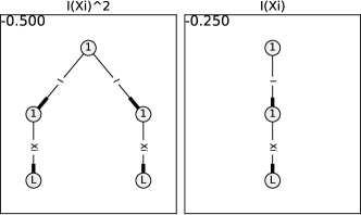
Figure 5: Negative homogeneity elements in the model space ${\mathcal{T}}_{F}$ for a quadratic polynomial $f$ ($N=2$), in dimension $d=2$ and with exponent $\rho=1.5$ for the SPDE (1.1) with space-time white noise forcing $\xi$. The top left corner for each element gives the homogeneity up to a multiple of an arbitrarily small factor, i.e., $|{\mathcal{I}}_{\rho}(\Xi)^{2}|_{\mathfrak{s}}=-\frac{1}{2}+{\mathcal{O}}(\kappa)$ and $|{\mathcal{I}}_{\rho}(\Xi)|_{\mathfrak{s}}=-\frac{1}{4}+{\mathcal{O}}(\kappa)$ for $0<\kappa\ll 1$.

For an example consider Figure 5, which lists the elements of negative homogeneity for the case $N=2$, $\rho=1.5$ and space-time white noise. For additive noise, these elements illustrate that the key building blocks have to be mixtures of integration against the kernel and taking powers. In the notation, we always suppress the trivial element ${\bf 1}$ but the element will be marked on the vertices of the trees to emphasize the product structure at the vertices.

The computation has been carried out in the package ReSSy (Regularity Structures Symbolic Computation Package), which has recently been developed. The main algorithm to compute the regularity structure elements provided the inputs $N,d,\rho$ is the iterative procedure (4.11)–(4.13). The algorithm has two main input parameters given by:

• maxh = maximum homogeneity of elements to keep after one iteration,

• iter = total number of fixed point iteration steps performed.

Of course, we cannot set $\texttt{maxh}=+\infty$ or to be arbitrarily large since this would include all elements of the polynomial regularity structure. For small to medium size regularity structures, it is possible to calculate all elements of negative homogeneity but for very large structures we have to take into account the fact that we may miss some elements if both algorithmic parameters are not large enough. Here we decided to report the parameters for each larger computation to guarantee for the reproducibility of results.

6.1 Explicit Examples – Negative Homogeneity Elements

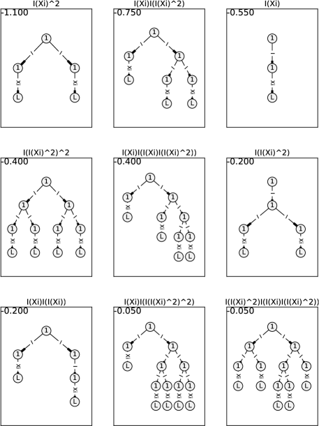
Figure 6: List of all negative-homogeneous elements in the basis ${\mathcal{F}}_{F}$ of the model space ${\mathcal{T}}_{F}$ for a quadratic polynomial $f$ ($N=2$), for dimension $d=2$ and with exponent $\rho=0.9$ for the SPDE (1.1) with space-time white noise forcing $\xi$. The corresponding pairs $(p,q)$ are shown in Figure 2.

In this section, we present a few more computational examples for space-time white noise. As shown in Section 4.2, it makes no practical sense to list all possible regularity structures. However, to build intuition, it is important to explicitly compute with key examples. In this regard, we must restrict the parameter space. Our main restriction is to consider

$$d\in\{2,3\}\;,\qquad N\in\{2,3\}\;.$$

The choice of dimension is motivated by the “classical physical” dimensions. $N>1$ is chosen since we are really interested in nonlinear problems. $N\mathrel{\leqsymb}3$ is motivated by classical normal form theory for ordinary differential equations [31], modulation/amplitude equations for partial differential equations [26] and stochastic partial differential equations [6]. In these contexts, one obtains normal forms near criticality with $N\mathrel{\leqsymb}3$ for the simplest codimension one bifurcations and pattern-forming mechanisms. For the fractional Laplacian parameter $\rho$, it makes sense to restrict to a regime

$$\rho\in(0,2]\bigcap\left\{\rho>\rho_{p}>\rho_{\rm{c}}=d\frac{N-1}{N+1}\right\}$$

where $\rho_{p}$ is a fixed number chosen as close as possible to the local subcriticality boundary but also fixed so that the computations are still possible in practice; indeed, we know from Section 4.2 that the model space grows very rapidly as we approach $\rho_{\rm{c}}$.

Figure 7: Examples of some negative homogeneity elements in the model space ${\mathcal{T}}_{F}$ for a cubic polynomial $f$ ($N=3$), for dimension $d=3$ and with exponent $\rho=1.7$ for the SPDE (1.1) with space-time white noise forcing $\xi$.

Figure 6 shows an example for $d=2=N$ and $\rho=0.9$ listing all elements of negative homogeneity. From the theory it is clear that the maximum degree of a vertex must be $N+1=3$. One easily checks that the pairs $(p,q)$ counting the number of $\Xi$ and ${\mathcal{I}}_{\rho}$ are compatible with the theory in Section 4.3, cf. Figure 2. Furthermore, in accordance with Proposition 4.17, all bare trees obtained by pruning the edges of type $\Xi$ are either binary trees, or can be turned into binary trees by adding one edge.

Figure 7 shows just four elements for a more complicated case with $d=3=N$ and $\rho=1.7$, where also nontrivial polynomial exponents appear; in this case, there are at least 42 negative homogeneity elements in ${\mathcal{F}}_{F}$ ($\texttt{iter}=4$, $\texttt{maxh}=2.0$). In accordance with Proposition 4.19, all pruned trees are either ternary trees, or ternary trees pruned by one edge.

6.2 Degree Distributions

The large dimension of the relevant sector of the model space may suggest that it is too complex to understand in detail. However, as already shown in Section 5, certain statistical properties become relevant as $\rho\searrow\rho_{\rm{c}}$.

\begin{overpic}[width=433.62pt]{./fig04} \put(40.0,68.0){(a)} \put(90.0,68.0){(b)} \put(40.0,30.0){(c)} \put(90.0,30.0){(d)} \end{overpic}

Figure 8: Computation of the degree distribution for the parameter values $N\in\{2,3\}$, $d\in\{2,3\}$ for negative homogeneous elements. Each histogram is coded according to a greyscale, i.e., black corresponds to the largest $\rho$-value used and $\rho=\rho_{p}$ corresponds to white. The degree distribution is visualized as a histogram normalized to the total number of elements of the regularity structure; note that we include the single trivial element ${\bf 1}$ with degree zero as it provides an indication of the absolute numbers in the normalized degree histogram. (a) Case $N=2=d$ (where $\rho_{\rm{c}}=\frac{2}{3}$), computed for $\texttt{maxh}=0.7$ and $\texttt{iter}=4$. The exponents for the fractional Laplacian are $\rho\in\{1.0,0.9,0.85,0.8,0.75,0.7\}$. (b) Case $N=2$, $d=3$, ($\rho_{\rm{c}}=1$), computed for $\texttt{maxh}=1.0$, $\texttt{iter}=4$ and $\rho\in\{1.4,1.3,1.25,1.2,1.15,1.1,1.08\}$. (c) Case $N=3$, $d=2$, ($\rho_{\rm{c}}=1$), computed for $\texttt{maxh}=1.0$, $\texttt{iter}=3$ and $\rho\in\{1.4,1.3,1.25,1.2,1.15,1.1,1.08\}$. (d) Case $N=3=d$, ($\rho_{\rm{c}}=\frac{3}{2}$), computed for $\texttt{maxh}=1.0$, $\texttt{iter}=3$ and $\rho\in\{1.8,1.75,1.7,1.65,$ $1.6,1.59\}$.

We start by considering the degree distribution $D$. Let ${\mathcal{R}}$ denote the set of rooted trees forming the set ${\mathcal{F}}_{F}^{-}$ of negative-homogeneous basis elements. Note that we can also view ${\mathcal{R}}$ as a single graph. Then we define

$$D(j;\rho)=\frac{\text{number of vertices of degree $j$ in ${\mathcal{R}}$}}{\text{ total number of vertices in ${\mathcal{R}}$}}=\frac{m_{j}}{m}\;.$$ (6.1)

Note that this is slightly different from the $D_{j}$ defined in Section 5.3, but both quantities are strongly related and converge to the same deterministic limit as $\rho\searrow\rho_{\rm{c}}$. In particular, it follows from (5.12) that $D(j;\rho)=\mathbb{E}[D_{j}(P+Q+1)]/\mathbb{E}[P+Q+1]$.

Figure 8 shows the degree distribution for the classical Allen–Cahn case with $N,d\in\{2,3\}$ for different values of $\rho$ approaching the subcriticality boundary at $d(N-1)/(N+1)=\rho_{\rm{c}}$; obviously we always consider this limit as a limit from above. Although $m\rightarrow+\infty$ as $\rho\rightarrow\rho_{\rm{c}}$, we see that the degree distribution $D(k;\rho)$ has relatively stable features. The trivial graph of the unit element ${\bf 1}$ explains the results at degree zero. The results are compatible with Proposition 5.4, which implies that the degrees should converge to $(\frac{1}{3},\frac{1}{3},\frac{1}{3})$ for $N=2$, and to $(\frac{2}{5},\frac{2}{5},0,\frac{1}{5})$ for $N=3$.

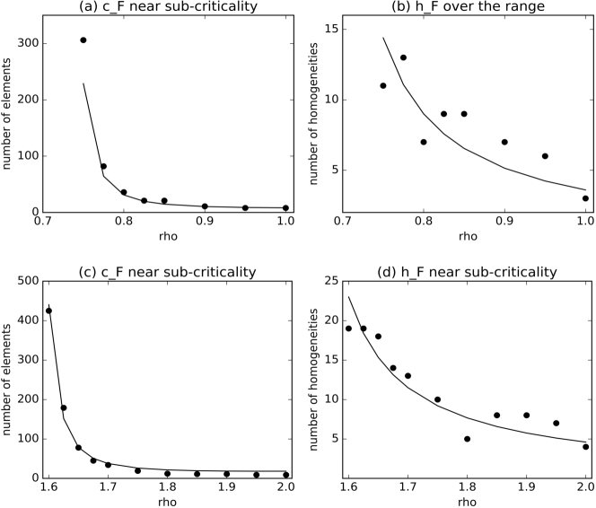
Figure 9: Computation to analyse the functions $h_{F}$ and $c_{F}$. Dots mark computational results while connected curves are theoretical scaling laws plotted using a least-square fit to the theoretical scaling laws. (a)–(b) Result for $N=2=d$ computed with $\texttt{maxh}=0.7$, $\texttt{iter}=5$. (c)–(d) Result for $N=3=d$ computed for $\texttt{maxh}=0.8$, $\texttt{iter}=4$.

Furthermore, we are also interested in the growth of the functions $c_{F}$ and $h_{F}$. The results of this computation are shown in Figure 9 for the cases $N=2=d$ and $N=3=d$. The results are compatible with the asymptotic growth in $(\rho-\rho_{\rm{c}})^{-1}$ of $h_{F}$ obtained in Theorem 4.12 and with the exponential growth of $c_{F}$ obtained in Theorems 4.18 and 4.20.

We briefly summarize some computational observations. Obviously, the results for the function $h_{F}$ are a lot easier to obtain computationally as we only need a large enough sub-sample of the entire model space to count homogeneities while for $c_{F}$, we have to count all elements (up to homogeneities equal to a multiple of $-\alpha_{0}$). Counting all elements requires higher values for iter and maxh, which can substantially increase the computation time. The key computational bottleneck, where the computation is slow, arises in the decision step whether during, or after, the construction of an element, this element is already contained in the model space from a previous iteration step. This step is unavoidable and necessitates a comparison to previously computed elements. The larger the individual graphs become, the more computationally intensive the computation may be. Note that we already reduce the computation time significantly by doing comparison by exclusion, e.g., first comparing the homogeneity, then comparing the number of edges and nodes, etc., until we finally have to check for complete graph isomorphism. Checking for graph isomorphism many times is extremely expensive so it should be avoided as much as possible.

6.3 Average Graph Properties

Although the degree distribution helps already to understand the approach towards the subcriticality boundary, it is also very interesting to consider other averaged graph properties.

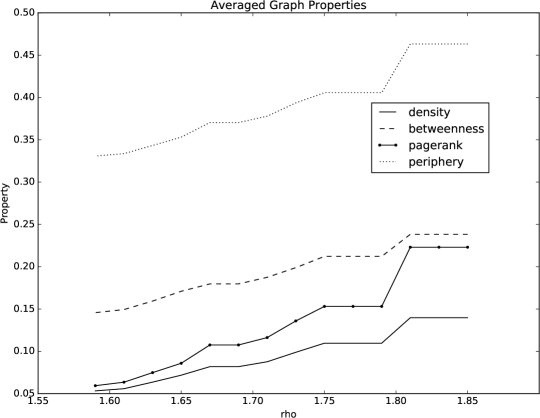
Figure 10: Computation of different averaged graph properties (vertical axis) for the regularity structure of the case $d=3=N$ for different values of $\rho$ (horizontal axis); the computation has been carried out for $\texttt{maxh}=1.5$ and $\texttt{iter}=3$. The properties are defined in the text but one can already see that density $M_{d}$ and pagerank $M_{r}$ are very close to zero at the subcriticality boundary; periphery $M_{p}$ and betweenness $M_{b}$ are decreasing but are more likely to stabilize at the subcriticality boundary $\rho=\frac{3}{2}$ to finite nonzero values.

As before, we let ${\mathcal{R}}$ denote the set of rooted trees spanning the negative-homogeneous sector ${\mathcal{F}}_{F}^{-}$ of the model space and let $|{\mathcal{R}}|=c_{F}$ denote the number of trees in ${\mathcal{R}}$. Then we consider the following properties of ${\mathcal{R}}$:

• Density: For an element $R\in{\mathcal{R}}$, let $n_{R}$ be the number of vertices in $R$ and $m_{R}$ be the number of edges in $R$. Then the graph density averaged over ${\mathcal{R}}$ is defined as

  $$M_{d}:=\frac{1}{|{\mathcal{R}}|}\sum_{R\in{\mathcal{R}}}\frac{m_{R}}{n_{R}(n_{R}-1)}\;.$$ (6.2)

  Since each $R$ is a tree, we have $n_{R}=m_{R}+1$ and thus $M_{d}$ is just the average of $1/n_{R}$, which we know to be of order $\rho-\rho_{\rm{c}}$. Hence, we expect it to decay to zero as $\rho\rightarrow\rho_{c}$.

• Betweenness: Let $\textnormal{path}(v_{1},v_{2})$ denote the number of shortest paths between two vertices $v_{1}$ and $v_{2}$ and let $\textnormal{path}(v_{1},v_{2}|v)$ denote the number of shortest paths that also pass through $v$; let $V_{R}$ denote the set of vertices of $R$. The betweenness (or betweenness centrality) averaged over ${\mathcal{R}}$ is defined as

  $$M_{b}:=\frac{1}{|{\mathcal{R}}|}\sum_{R\in{\mathcal{R}}}\frac{1}{n_{R}}\sum_{v\in R}\sum_{v_{1},v_{2}\in V_{R}}\frac{\textnormal{path}(v_{1},v_{2}|v)}{\textnormal{path}(v_{1},v_{2})}\;.$$ (6.3)

  Since each $R$ is a tree, $\textnormal{path}(v_{1},v_{2})=1$. However, betweenness centrality for trees is still a property not fully understood [14] so it is of interest to just calculate it here.

• PageRank: Let $\textnormal{pagerank}(v)$ denote the pagerank of a node computed according to [36], which measures the importance of a vertex in a graph. Then the averaged PageRank is defined as

  $$M_{r}:=\frac{1}{|{\mathcal{R}}|}\sum_{R\in{\mathcal{R}}}\frac{1}{n_{R}}\sum_{v\in R}\textnormal{pagerank}(v)\;.$$ (6.4)

• Periphery: For $R\in{\mathcal{R}}$ let $|\textnormal{ecc}_{R}|$ be the number of vertices in $R$ with eccentricity equal to the diameter of $R$; recall that the eccentricity of a vertex $v$ is the maximum distance from $v$ to all other vertices and the diameter of a graph is the maximum eccentricity over all nodes. Then the averaged periphery measure is defined as:

  $$M_{p}:=\frac{1}{|{\mathcal{R}}|}\sum_{R\in{\mathcal{R}}}|\textnormal{ecc}_{R}|\;.$$ (6.5)

Note that for $M_{b}$ and $M_{r}$, we view each rooted tree as an undirected graph, while the computations are for directed graphs for $M_{d}$ and $M_{p}$. The graph properties are essentially coarse-grained summary statistics of the set of rooted trees ${\mathcal{R}}$ and represent different characteristics. Figure 10 shows a computation for the benchmark case fixing $d=3=N$ and leaving $\rho$ to vary. The density $M_{d}$ decreases as expected. The averaged betweenness $M_{b}$ also decreases as $\rho$ decreases but seems to stabilize to a finite value, i.e., there is a typical shortest path scale developing. The PageRank $M_{r}$ was designed to measure the importance/connectedness of vertices and it also becomes very small as $\rho\rightarrow\frac{3}{2}$. This indicates that although each rooted tree is quite structured, it still grows individually in such a way to produce only a few special or significant nodes so that the effect of $|{\mathcal{R}}|$ increasing eventually dominates. Quite interestingly, the averaged periphery measure $M_{p}$ also seems to have a well-defined finite value near subcriticality. $M_{p}$ essentially measures how many nodes are in the periphery of the trees and this indicates that the growth of the rooted trees does follow a pattern still adding a lot of smaller trees at the ends rather than maximizing connectedness.

6.4 Homogeneity Distribution

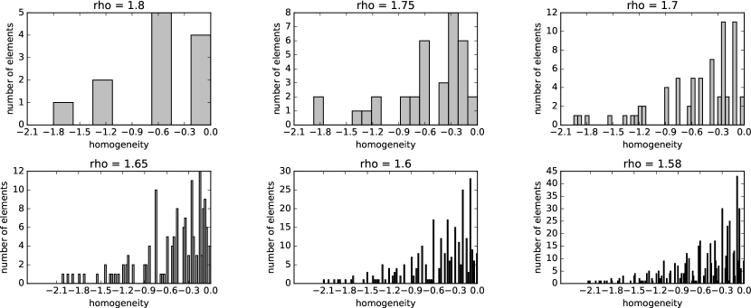
Figure 11: Computation of homogeneity distributions for the regularity structure $d=3=N$ for different values of $\rho\in\{1.8,1.75,1.7,1.65,1.6,1.58\}$, where each histogram shows the number of elements in the regularity structure sorted according to negative homogeneity but discarding arbitrarily small factors in $|\cdot|_{\mathfrak{s}}=\cdot+{\mathcal{O}}(\kappa)$, i.e., dropping the terms of order ${\mathcal{O}}(\kappa)$ as $\kappa>0$ is arbitrarily small. The computation has been carried out for $\texttt{maxh}=1.5$ and $\texttt{iter}=3$.

Another important measure for rooted trees in ${\mathcal{F}}_{F}^{-}$ is their homogeneity, i.e., we consider $\mathfrak{H}(R)={}|R|_{\mathfrak{s}}$ for $R\in{\mathcal{R}}$ by just viewing the rooted tree as a symbol.

Figure 11 again shows results for our benchmark case $d=3=N$ for different values of $\rho$. Each histogram counts the number of elements of a given homogeneity and each bin in the histogram is just one homogeneity level. Note that we could have normalized the histograms by $|{\mathcal{R}}|$ to obtain a probability distribution, but the absolute counts are also informative and we have scaled the vertical axis so that one already sees the normalized versions. The results are consistent with Proposition 5.3, and in particular with the large-deviation estimate (5.11) showing that the probability of the homogeneity having a negative value $h$ behaves like $\operatorname{e}^{-\kappa(-h)/(\rho-\rho_{\rm{c}})}$. Another observation from Figure 11 is that upon decreasing $\rho$, new homogeneities appear in a very regular fashion, at least reminiscent of the construction of functions with fractal graphs. Indeed, if $\rho$ is rational, then only rational negative homogeneities may appear by the iterative construction. However, the negative homogeneities really do seem to fill out an entire domain of $\rho$.

Nils Berglund
Université d’Orléans, Laboratoire Mapmo, CNRS, UMR 7349
Fédération Denis Poisson, FR 2964
Bâtiment de Mathématiques, B.P. 6759
45067 Orléans Cedex 2, France
E-mail address: nils.berglund@univ-orleans.fr

Christian Kuehn
Technical University of Munich (TUM)
Faculty of Mathematics
Boltzmannstr. 3
85748 Garching bei München, Germany
E-mail address: ckuehn@ma.tum.de

References

- [1] F. Achleitner and C. Kuehn. Traveling waves for a bistable equation with nonlocal-diffusion. Adv. Differential Equat., 20(9):887–936, 2015.
- [2] S.M. Allen and J.W. Cahn. A microscopic theory for antiphase boundary motion and its application to antiphase domain coarsening. Acta Metallurgica, 27(6):1085–1905, 1979.
- [3] L. Arnold. Random Dynamical Systems. Springer, Berlin Heidelberg, Germany, 2003.
- [4] N. Berglund, G. Di Gesù, and H. Weber. An Eyring-Kramers law for the stochastic Allen-Cahn equation in dimension two. arXiv:1604.05742, pages 1–26, 2016.
- [5] N. Berglund and C. Kuehn. Regularity structures and renormalisation of FitzHugh-Nagumo SPDEs in three space dimensions. Electron. J. Probab., 21(18):1–48, 2016.
- [6] D. Blömker. Amplitude Equations for Stochastic Partial Differential Equations. World Scientific, 2007.
- [7] Nicolas Broutin and Philippe Flajolet. The distribution of height and diameter in random non-plane binary trees. Random Structures Algorithms, 41(2):215–252, 2012.
- [8] Y. Bruned, M. Hairer, and L. Zambotti. Algebraic renormalisation of regularity structures. arXiv:1610.08468, pages 1–84, 2016.
- [9] A. Chandra and M. Hairer. An analytic BPHZ theorem for regularity structures. arXiv:1612.08138, pages 1–113, 2016.
- [10] Ajay Chandra and Hendrik Weber. Stochastic PDEs, regularity structures, and interacting particle systems. arXiv:1508.03616, 2015.
- [11] Z.-Q. Chen, P. Kim, and R. Song. Heat kernel estimates for the Dirichlet fractional Laplacian. J. Eur. Math. Soc., 12:1307–1329, 2010.
- [12] M.C. Cross and P.C. Hohenberg. Pattern formation outside of equilibrium. Rev. Mod. Phys., 65(3):851–1112, 1993.
- [13] C.M. Dafermos. Hyperbolic Conservation Laws in Continuum Physics. Springer, 2010.
- [14] B. Fish, R. Kushwaha, and G. Turan. Betweenness centrality profiles in trees. arXiv:1607.02334, pages 1–21, 2016.
- [15] R.A. Fisher. The wave of advance of advantageous genes. Ann. Eugenics, 7:353–369, 1937.
- [16] P.K. Friz and M. Hairer. A Course on Rough Paths: With an Introduction to Regularity Structures. Springer, 2014.
- [17] C. Gardiner. Stochastic Methods. Springer, Berlin Heidelberg, Germany, 4th edition, 2009.
- [18] M. Gubinelli. Controlling rough paths. J. Funct. Anal., 216(1):86–140, 2004.
- [19] M. Gubinelli, P. Imkeller, and N. Perkowski. Paracontrolled distributions and singular PDEs. Forum Math. Pi, 3:e6, 2015.
- [20] M. Gubinelli and S. Tindel. Rough evolution equations. Ann. Probab., 38:1–75, 2010.
- [21] M. Hairer. Solving the KPZ equation. Ann. Math., 178(2):559–664, 2013.
- [22] M. Hairer. A theory of regularity structures. Invent. Math., 198(2):269–504, 2014.
- [23] M. Hairer. The motion of a random string. arXiv:1605.02192, pages 1–20, 2015.
- [24] M. Hairer. Regularity structures and the dynamical model. arXiv:1508.05261, pages 1–46, 2015.
- [25] M. Hairer and H. Weber. Large deviations for white-noise driven, nonlinear stochastic PDEs in two and three dimensions. Ann. Fac. Sci. Toulouse Math., 24(1):55–92, 2015.
- [26] R. Hoyle. Pattern Formation: An Introduction to Methods. Cambridge University Press, 2006.
- [27] J.-M-Bony. Calcul symbolique et propagation des singularites pour les équations aux dérivées partielles non linéaires. Ann. Sci. Ec. Norm. Super., 4(14):209–246, 1981.
- [28] M. Kardar, G. Parisi, and Y.C. Zhang. Dynamic scaling of growing interfaces. Phys. Rev. Lett., 56(9):889–892, 1986.
- [29] R. Klages, G. Radons, and I.M. Sokolov. Anomalous Transport: Foundations and Applications. Wiley, 2008.
- [30] A. Kolmogorov, I. Petrovskii, and N. Piscounov. A study of the diffusion equation with increase in the amount of substance, and its application to a biological problem. In V.M. Tikhomirov, editor, Selected Works of A. N. Kolmogorov I, pages 248–270. Kluwer, 1991. Translated by V. M. Volosov from Bull. Moscow Univ., Math. Mech. 1, 1–25, 1937.
- [31] Yu.A. Kuznetsov. Elements of Applied Bifurcation Theory. Springer, New York, NY, 3rd edition, 2004.
- [32] M. Kwaśnicki. Ten equivalent definitions of the fractional Laplace operator. arXiv:1507.07356, pages 1–31, 2015.
- [33] R. Metzler and J. Klafter. The random walk’s guide to anomalous diffusion: a fractional dynamics approach. Phys. Rep., 339(1):1–77, 2000.
- [34] J. Nagumo, S. Arimoto, and S. Yoshizawa. An active pulse transmission line simulating nerve axon. Proc. IRE, 50:2061–2070, 1962.
- [35] Richard Otter. The number of trees. Ann. of Math. (2), 49:583–599, 1948.
- [36] L. Page, S. Brin, R. Motwani, and T. Winograd. The PageRank citation ranking: bringing order to the web. http://ilpubs.stanford.edu:8090/422/1/1999-66.pdf, pages 1–17, 1999.
- [37] G. Da Prato and J. Zabczyk. Stochastic Equations in Infinite Dimensions. Cambridge University Press, 1992.
- [38] K. Sato. Lévy Processes and Infinitely Divisible Distributions. CUP, 1999.