Model reduction of a kinetic swarming model by operator projection

Abstract

This paper derives the arbitrary order globally hyperbolic moment system for a non-linear kinetic description of the Vicsek swarming model by using the operator projection. It is built on our careful study of a family of the complicate Grad type orthogonal functions depending on a parameter (angle of macroscopic velocity). We calculate their derivatives with respect to the independent variable, and projection of those derivatives, the product of velocity and basis, and collision term. The moment system is also proved to be hyperbolic, rotational invariant, and mass-conservative. The relationship between Grad type expansions in different parameter is also established. A semi-implicit numerical scheme is presented to solve a Cauchy problem of our hyperbolic moment system in order to verify the convergence behavior of the moment method. It is also compared to the spectral method for the kinetic equation. The results show that the solutions of our hyperbolic moment system converge to the solutions of the kinetic equation for the Vicsek model as the order of the moment system increases, and the moment method can capture key features such as vortex formation and traveling waves.

Keywords: Moment method, hyperbolicity, kinetic equation, model reduction, operator projection

1 Introduction

Swarm behaviour, or swarming, is a collective behaviour exhibited by entities, particularly animals, of similar size which aggregate together, perhaps milling about the same spot or perhaps moving en masse or migrating in some direction [1]. It is a highly interdisciplinary topic. Some works studied kinetic models for swarming [7, 10, 17], but few did a numerical investigation. The first numerical method was presented in [13] for a kinetic description of the Vicsek swarming model. The main contribution was to use a spectral representation linked with a discrete constrained optimization to compute those interactions. Unfortunately, only first-order accurate upwind method was used to approximated the transport term.

The kinetic theory has been widely studied and played an important role in many fields during several decades, see e.g. [8, 9]. The kinetic equation can determine the distribution function hence the transport coefficients, however such task is not so easy. The moment method [15, 16] is a model reduction for the kinetic equation by expanding the distribution function in terms of tensorial Hermite polynomials and introducing the balance equations corresponding to higher order moments of the distribution function. One major disadvantage of the Grad moment method is the loss of hyperbolicity, which will cause the solution blow-up when the distribution is far away from the equilibrium state. Increasing the number of moments could not avoid such blow-up [6]. Up to now, there has been some latest progress on the Grad moment method for the kinetic equation. Numerical regularized moment method of arbitrary order was studied for Boltzmann-BGK equation [5] and for high Mach number flow [6]. Based on the observation that the characteristic polynomial of the flux Jacobian in the Grad moment system did not depend on the intermediate moments, a regularization was presented in [2, 3, 4] for the one- and multi-dimensional Grad moment systems to achieve global hyperbolicity. The quadrature based projection methods were used to derive hyperbolic systems for the solution of the Boltzmann equation [18, 19] by using the quadrature rule instead of the exact integration. In the 1D case, it is similar to the regularization in [2]. Those contributions led to well understanding the hyperbolicity of the Grad moment systems. Based on the operator projection, a general framework of model reduction technique was recently given in [12]. It projected the time and space derivatives in the kinetic equation into a finite-dimensional weighted polynomial space synchronously, and could give most of the existing moment systems in the literature. Recently, such model reduction method was also successfully extended to the 1D special relativistic Boltzmann equation and the globally hyperbolic moment model of arbitrary order was derived in [20].

The aim of this paper is to extend the model reduction method by the operator projection to the two-dimensional kinetic description of the Vicsek swarming model and derive corresponding globally hyperbolic moment system of arbitrary order. The paper is organized as follows. Section 2 introduces the kinetic and macroscopic equations for the Vicsek model. Section 3 gives a family of orthogonal functions dependent on a parameter and their properties and derives the arbitrary order globally hyperbolic moment system of the kinetic description for the Vicsek model. Section 4 investigates the mathematical properties of moment system, including: hyperbolicity, rotational invariance, mass-conservation and relationship between Grad type expansions in different parameter. Section 5 presents a semi-implicit numerical scheme and conducts a numerical experiment to check the convergence of the proposed hyperbolic moment system. Section 6 concludes the paper.

2 Kinetic and macroscopic equations for the Vicsek model

This section introduces the non-linear kinetic and macroscopic equations for the Vicsek model.

2.1 Kinetic equation

The kinetic equation for the Vicsek model can be written as follows [13]

$$\partial_{t}f +\mbox{\boldmath\small$\omega$}\cdot{\nabla_{\boldsymbol{x}}}f+{\nabla_{\mbox{\boldmath\small$\omega$}}}\cdot(\mbox{\boldmath\small$F$}[f]f)=\sigma\Delta_{\mbox{\boldmath\small$\omega$}}f,$$ (2.1)

where $f(t,\boldsymbol{x},\mbox{\boldmath\small$\omega$})$ is the particle distribution function depending on the time $t$, spatial variable $\boldsymbol{x}\in\mathbb{R}^{d}$, and the unit velocity vector $\omega$, the parameter $\sigma$ is a scaled diffusion constant describing the intensity of the noise with the Brownian motion, the vector $\mbox{\boldmath\small$F$}[f](t,\mbox{\boldmath\small$x$},\mbox{\boldmath\small$\omega$})$ is the mean-field interaction force between the particles and given by

$$\mbox{\boldmath\small$F$}[f](t,\boldsymbol{x},\mbox{\boldmath\small$\omega$})= (\mathrm{Id}-\mbox{\boldmath\small$\omega$}\otimes\mbox{\boldmath\small$\omega$})\mbox{\boldmath\small$\Omega$}(\boldsymbol{x}),\quad\mbox{\boldmath\small$\Omega$}(t,\boldsymbol{x})=\dfrac{\mbox{\boldmath\small$J$}(t,\boldsymbol{x})}{\lvert\mbox{\boldmath\small$J$}(t,\boldsymbol{x})\rvert},$$ (2.2)

the notation $\mathrm{Id}$ is the identity operator, $\mbox{\boldmath\small$\Omega$}(t,\boldsymbol{x})$ is the mean velocity, and $\mbox{\boldmath\small$J$}(t,\boldsymbol{x})$ denotes the mean flux at $x$ and is defined by

$$\mbox{\boldmath\small$J$}(t,\boldsymbol{x})= \int_{\mathbb{R}^{d}}\int_{S^{d-1}}K(\boldsymbol{y}-\boldsymbol{x})\mbox{\boldmath\small$\omega$}f(t,\boldsymbol{y},\mbox{\boldmath\small$\omega$})\mathrm{d}\boldsymbol{y}\mathrm{d}\mbox{\boldmath\small$\omega$}.$$ (2.3)

Here $K(\boldsymbol{y}-\boldsymbol{x})$ is the characteristic function of the ball $B(0,R)=\{\mbox{\boldmath\small$x$}:|\mbox{\boldmath\small$x$}|\leq R\}$, i.e. $K(\mbox{\boldmath\small$x$})={\boldsymbol{1}}_{\lvert\mbox{\boldmath\small$x$}\rvert<R}$, and $R$ is the radius of the alignment interactions between the particles. The vector field $\mbox{\boldmath\small$F$}[f](t,\mbox{\boldmath\small$x$},\mbox{\boldmath\small$\omega$})$ tends to align the particles to the direction $\Omega$ which is the director of the particle flux $J$ and becomes spatially local in the large scale limit of space and time so that $J$ can be approximated by

$$\mbox{\boldmath\small$J$}(t,\boldsymbol{x})=\int_{S^{d-1}}\mbox{\boldmath\small$\omega$}f(t,\boldsymbol{x},\mbox{\boldmath\small$\omega$})\mathrm{d}\mbox{\boldmath\small$\omega$}.$$ (2.4)

In the numerical computations, $\mbox{\boldmath\small$J$}(t,\boldsymbol{x})$ can be considered within the approximation (2.4) because the spatial mesh stepsize may be smaller than the radius of ball $B(0,R)$ [13].

It has been shown [14] that the non-linear kinetic equation (2.1) with (2.2) and (2.3) or (2.4) has a non-negative global weak solution in $C(0,T;L^{1}(D)\cap L^{\infty}\big{(}(0,T)\times D\big{)}$ with $D=\mathbb{R}^{d}\times S^{d-1}$, for any time $T$, given non-negative initial value $f(0,\boldsymbol{x},\mbox{\boldmath\small$\omega$})$ in $L^{1}(D)\cap L^{\infty}(D)$ and $\mbox{\boldmath\small$J$}(t,\boldsymbol{x})$ which is always not equal to $\mathrm{0}$ for $t\in[0,T]$.

Throughout the paper, we will only consider the case of (2.4) and the direction of mean velocity of $f$ becomes

$$\mbox{\boldmath\small$\Omega$}=\dfrac{\int_{S^{d-1}}\mbox{\boldmath\small$\omega$}f\mathrm{d}\mbox{\boldmath\small$\omega$}}{\lvert\int_{S^{d-1}}\mbox{\boldmath\small$\omega$}f\mathrm{d}\mbox{\boldmath\small$\omega$}\rvert}.$$

Moreover, the kinetic equation (2.1) is rewritten as following

$$\partial_{t}f+\mbox{\boldmath\small$\omega$}\cdot\nabla_{\boldsymbol{x}}f=Q(f),$$ (2.5)

where the collision term $Q(f)$ is defined by

$$Q(f)=-{\nabla_{\mbox{\boldmath\small$\omega$}}}\cdot(\mbox{\boldmath\small$F$}[f]f)+\sigma\Delta_{\mbox{\boldmath\small$\omega$}}f.$$ (2.6)

Lemma 1 ([13]).

The collision term $Q(f)$ can be rewritten as follows

$$Q(f)=\sigma\nabla_{\mbox{\boldmath\small$\omega$}}\cdot\left(M_{\mbox{\boldmath\small$\Omega$}}\nabla_{\mbox{\boldmath\small$\omega$}}\big{(}\dfrac{f}{M_{\mbox{\boldmath\small$\Omega$}}}\big{)}\right),$$ (2.7)

and satisfies

$$\int_{S^{d-1}}Q(f)f\frac{\mathrm{d}\mbox{\boldmath\small$\omega$}}{M_{\mbox{\boldmath\small$\Omega$}}}\leq 0,$$ (2.8)

where

$$M_{\mbox{\boldmath\small$\Omega$}}(\mbox{\boldmath\small$\omega$})=C_{0}\exp(\dfrac{\mbox{\boldmath\small$\omega$}\cdot\mbox{\boldmath\small$\Omega$}}{\sigma}),$$ (2.9)

is the equilibrium function, also known as the Von Mises distribution, and $C_{0}$ is a constant of normalization.

Remark 2.1.

The equilibria of operator $Q$ are given by the set $\{\rho M_{\mbox{\boldmath\small$\Omega$}}|\rho\in\mathbb{R},\mbox{\boldmath\small$\Omega$}\in S^{d-1}\}$ and forms a set of dimension $d$, but the collisional invariants of $Q$ are only of dimension 1. Particularly, $Q$ does preserve the mass but cannot preserve the flux, that is, for a general $f$, it holds

$$\int_{S^{d-1}}Q(f)\mathrm{d}\mbox{\boldmath\small$\omega$}=0,\quad\int_{S^{d-1}}Q(f)\mbox{\boldmath\small$\omega$}\mathrm{d}\mbox{\boldmath\small$\omega$}\neq 0.$$

Remark 2.2.

In the case of $d=2$, if letting $\mbox{\boldmath\small$\Omega$}=(\cos\bar{\theta},\sin\bar{\theta})^{T}$, then the equilibrium can be expressed as follows

$$M(\theta-\bar{\theta})=C_{0}\exp\left(\dfrac{\cos(\theta-\bar{\theta})}{\sigma}\right),$$ (2.10)

and the kinetic equation (2.5) becomes

$$f_{t} +\cos\theta f_{x}+\sin\theta f_{y}=Q(f),$$ (2.11)

$$Q(f)= \sigma\partial_{\theta}\left(M_{\bar{\theta}}\partial_{\theta}\big{(}\dfrac{f}{M_{\bar{\theta}}}\big{)}\right)=\partial_{\theta}(\sin(\theta-\bar{\theta})f)+\sigma\partial_{\theta}^{2}f,$$

where  $\theta$ and $\bar{\theta}$ denote the angles of microscopic and macroscopic velocities, respectively.

2.2 Macroscopic equations

The kinetic equation (2.5) is written at the microscopic level, i.e. at time and length scales which are characteristic of the dynamics of the individual particles. When investigating the dynamics of the system at large time and length scales compared with the scales of the individuals, a set of new variables $\tilde{t}=\varepsilon t$ and $\tilde{\boldsymbol{x}}=\varepsilon\boldsymbol{x}$ has to be introduced [11], where $\varepsilon$ denotes the ratio between micro and macro variables, $\varepsilon\ll 1$. In this new set of variables, the kinetic equation (2.5) is written (after dropping the tildes for clarity) as follows

$$\partial_{t}f^{\varepsilon}+\mbox{\boldmath\small$\omega$}\cdot{\nabla_{\boldsymbol{x}}}f^{\varepsilon}=\dfrac{1}{\varepsilon}Q(f^{\varepsilon}).$$ (2.12)

In the limit $\varepsilon\rightarrow 0$,  $f^{\varepsilon}$ converges locally in space to an equilibrium state in the local space, that is

$$f^{\varepsilon}\rightarrow f(t,\boldsymbol{x},\mbox{\boldmath\small$\omega$})=\rho(t,\boldsymbol{x})M_{\mbox{\boldmath\small$\Omega$}}(\mbox{\boldmath\small$\omega$}).$$ (2.13)

At this moment, the evolution of macroscopic density $\rho=\int_{S^{d-1}}f\mathrm{d}\mbox{\boldmath\small$\omega$}$ and velocity $\Omega$ is described by the following equations

$$\partial_{t}\rho+\nabla_{\boldsymbol{x}}\cdot(c_{1}\rho\mbox{\boldmath\small$\Omega$})=0,$$ (2.14)

$$\rho(\partial_{t}\mbox{\boldmath\small$\Omega$}+c_{2}(\mbox{\boldmath\small$\Omega$}\cdot\nabla_{\boldsymbol{x}})\mbox{\boldmath\small$\Omega$})+\lambda(\mathrm{Id}-\mbox{\boldmath\small$\Omega$}\otimes\mbox{\boldmath\small$\Omega$})\nabla_{\boldsymbol{x}}\rho=0,$$ (2.15)

$$\lvert\mbox{\boldmath\small$\Omega$}\rvert=1,$$ (2.16)

where $c_{1},c_{2}$, and $\lambda$ are three constants depending on $\sigma$. Such macroscopic system is hyperbolic but non-conservative, and the operator $\mathrm{Id}-\mbox{\boldmath\small$\Omega$}\otimes\mbox{\boldmath\small$\Omega$}$ ensures the constraint (2.16).

Remark 2.3.

In the 2D case, the macroscopic density $\rho$ and angle of velocity $\bar{\theta}$ are related to the particle distribution function $f$ by

$$\rho(t,\boldsymbol{x})=\int_{0}^{2\pi}f(t,\boldsymbol{x},\theta)\mathrm{d}\theta,$$ (2.17a)

$$\mbox{\boldmath\small$J$}(t,\boldsymbol{x})=\int_{0}^{2\pi}\begin{pmatrix}\cos\theta\\ \sin\theta\end{pmatrix}f(t,\boldsymbol{x},\theta)\mathrm{d}\theta,$$ (2.17b)

$$\mbox{\boldmath\small$\Omega$}=(\cos\bar{\theta},\sin\bar{\theta})^{T}=\dfrac{\mbox{\boldmath\small$J$}(t,\boldsymbol{x})}{\lvert\mbox{\boldmath\small$J$}(t,\boldsymbol{x})\rvert}.$$ (2.17c)

3 Derivation of moment system

This section derives the moment system for the 2D kinetic description of Vicsek swarming model by using the operator projection [12, 20]. For the sake of simplicity, we assume $\bar{\theta}=0$ in Sections 3.1 and 3.2. In fact, the general case of $\bar{\theta}\not=0$ can be converted into such simple case by operating a translation transformation $\theta\mapsto\theta-\bar{\theta}$.

3.1 Orthogonal functions

The Hermite polynomials are used to derive the Grad’s moment system [15, 16], where the distribution function is assumed to close to a local Maxwellian. Here we need to find the orthogonal functions with respect to the weight $M(\theta)$ defined in $[0,2\pi]$, because $\theta\in[0,2\pi]$. Those functions, denoted by

$$H^{c}_{0}(\theta),H^{c}_{1}(\theta),\cdots,H^{c}_{N}(\theta),\cdots,H^{s}_{1}(\theta),\cdots,H^{s}_{N}(\theta),\cdots,$$

are built on the trigonometric functions

$$\{1,\cos\theta,\cdots,\cos(N\theta),\cdots;\sin\theta,\cdots,\sin(N\theta),\cdots\}$$

by using the Schmit orthogonal process, where the superscript $c$ (resp. $s$) denotes the functions consisting of a linear combination of $\cos(k\theta)$ (resp. $\sin(k\theta)$). Because the function $M(\theta)$ is even, it holds

$$\int_{0}^{2\pi}\sin(m\theta)\cos(n\theta)M(\theta)\mathrm{d}\theta=0,\quad\forall m,n\in\mathbb{N},$$

so in the process of Schimidt orthogonalization, the linear combination of $\cos(k\theta)$ is orthogonal to that of $\sin(k\theta)$, so that there are two sets of “independent” orthogonal functions. The first $2N+1$ functions are $H^{c}_{0}(\theta),H^{c}_{1}(\theta),\cdots,H^{c}_{N}(\theta)$ and $H^{s}_{1}(\theta),\cdots,H^{s}_{N}(\theta)$, and can be expressed in terms of the trigonometric functions $\{1,\cos\theta,\cdots,\cos(N\theta)$,  $\sin\theta,\cdots,\sin(N\theta)\}$ as follows

$$\begin{pmatrix}H^{c}_{0}(\theta),H^{c}_{1}(\theta),\cdots,H^{c}_{N}(\theta)\\ \end{pmatrix}^{\mathrm{T}}=A_{N}\begin{pmatrix}1,\cos\theta,\cdots,\cos(N\theta)\\ \end{pmatrix}^{\mathrm{T}},$$ (3.1)

$$\begin{pmatrix}H^{s}_{1}(\theta),\cdots,H^{s}_{N}(\theta)\\ \end{pmatrix}^{\mathrm{T}}=B_{N}\begin{pmatrix}\sin\theta,\cdots,\sin(N\theta)\\ \end{pmatrix}^{\mathrm{T}},$$ (3.2)

where $A_{N}\in\mathbb{R}^{(N+1)\times(N+1)},B_{N}\in\mathbb{R}^{N\times N}$, and both $A_{N}$ and $B_{N}$ are invertible lower triangular matrix. This set of functions satisfy

$$\int_{0}^{2\pi}H^{l}_{m}(\theta)H^{l}_{n}(\theta)M(\theta)\mathrm{d}\theta=\delta_{m,n},\quad m,n\in\{0,1,\cdots,N\},l\in\{c,s\}.$$

When $l=s$, $m,n\not=0$. For the sake of simplicity, define

$$\begin{pmatrix}1,\cos\theta,\cdots,\cos(N\theta)\\ \end{pmatrix}^{\mathrm{T}}\triangleq\boldsymbol{E}^{c}_{N}(\theta),\ \ \begin{pmatrix}\sin\theta,\cdots,\sin(N\theta)\\ \end{pmatrix}^{\mathrm{T}}\triangleq\boldsymbol{E}^{s}_{N}(\theta),$$

$$\begin{pmatrix}H^{c}_{0}(\theta),H^{c}_{1}(\theta),\cdots,H^{c}_{N}(\theta)\\ \end{pmatrix}^{\mathrm{T}}\triangleq\boldsymbol{H}^{c}_{N}(\theta),\ \ \begin{pmatrix}H^{s}_{1}(\theta),H^{s}_{2}(\theta),\cdots,H^{s}_{N}(\theta)\\ \end{pmatrix}^{\mathrm{T}}\triangleq\boldsymbol{H}^{s}_{N}(\theta),$$

$$\begin{pmatrix}H^{c}_{0}(\theta),H^{c}_{1}(\theta),\cdots\\ \end{pmatrix}^{\mathrm{T}}\triangleq\boldsymbol{H}^{c}(\theta),\ \ \begin{pmatrix}H^{s}_{1}(\theta),H^{s}_{2}(\theta),\cdots\\ \end{pmatrix}^{\mathrm{T}}\triangleq\boldsymbol{H}^{s}(\theta),$$

then (3.1) and (3.2) can be rewritten as follows

$$\boldsymbol{H}^{c}_{N}(\theta)=A_{N}\boldsymbol{E}^{c}_{N}(\theta),\quad\boldsymbol{H}^{s}_{N}(\theta)=B_{N}\boldsymbol{E}^{s}_{N}(\theta).$$ (3.3)

It is worth noting that the first polynomial is 1, and will be applied to the calculation of density $\rho$.

Remark 3.1.

The coefficients $A_{N}$ and $B_{N}$ in (3.3) can be calculated by using the following regular modified cylindrical Bessel function of order $n$

$$I_{n}(x)=\dfrac{1}{\pi}\int_{0}^{\pi}\exp(x\cos\theta)\cos(n\theta)\mathrm{d}\theta.$$ (3.4)

In fact, because of the identities

$$\sin(m\theta)\sin(n\theta) =-\dfrac{1}{2}[\cos((m+n)\theta)-\cos((m-n)\theta)],$$

$$\cos(m\theta)\cos(n\theta) =\dfrac{1}{2}[\cos((m+n)\theta)+\cos((m-n)\theta)],$$

the Schmidt process is carried out with the aid of $I_{n}(x)$, and then the calculation of $A_{N}$ and $B_{N}$ is completed by the existing packages.

3.2 Hilbert space and orthonormal basis

On the interval $[0,2\pi]$, define Hilbert space $\mathcal{H}$ and inner product with respect to the weight $M(\theta)$ by

$${\mathcal{H}}=\left\{f\Big{|}\int_{0}^{2\pi}f^{2}(\theta)\frac{\mathrm{d}\theta}{M(\theta)}<\infty\right\},$$ (3.5)

$$\langle{f(\theta)},{g(\theta)}\rangle_{M(\theta)}\triangleq\int_{0}^{2\pi}f(\theta)g(\theta)\dfrac{\mathrm{d}\theta}{M(\theta)}.$$ (3.6)

Such inner product is symmetric, i.e.

$$\langle{f},{g}\rangle_{M(\theta)}=\langle{g},{f}\rangle_{M(\theta)}.$$

Moreover, due to (2.7), the inner product still satisfies

$$\langle{Q(f)},{g}\rangle_{M(\theta)}=-\sigma\int_{0}^{2\pi}M(\theta)\partial_{\theta}\left(\dfrac{f}{M}\right)\partial_{\theta}\left(\dfrac{g}{M}\right){\mathrm{d}\theta}=\langle{f},{Q(g)}\rangle_{M(\theta)},$$ (3.7)

and

$$\langle{Q(f)},{f}\rangle_{M(\theta)}=-\sigma\int_{0}^{2\pi}M(\theta)\partial_{\theta}^{2}\left(\dfrac{f}{M}\right){\mathrm{d}\theta}\leqslant 0.$$ (3.8)

Take a basis of $\mathcal{H}$ as $P^{c}_{0}(\theta),\cdots,P^{c}_{N}(\theta)\cdots$,  $P^{s}_{1}(\theta),\cdots,P^{s}_{N}(\theta)\cdots$, and denote

$$\begin{pmatrix}P^{c}_{0}(\theta),P^{c}_{1}(\theta),\cdots\\ \end{pmatrix}^{\mathrm{T}}\triangleq\boldsymbol{P}^{c}(\theta),$$ (3.9a)

$$\begin{pmatrix}P^{s}_{1}(\theta),P^{s}_{2}(\theta),\cdots\\ \end{pmatrix}^{\mathrm{T}}\triangleq\boldsymbol{P}^{s}(\theta).$$ (3.9b)

Such basis can be generated by the previous orthogonal functions $\boldsymbol{H}^{c}(\theta)$ and $\boldsymbol{H}^{s}(\theta)$ as follows

$$\boldsymbol{P}^{c}(\theta)=\boldsymbol{H}^{c}(\theta)M(\theta),\quad\boldsymbol{P}^{s}(\theta)=\boldsymbol{H}^{s}(\theta)M(\theta).$$ (3.10)

Lemma 2.

The functions $\boldsymbol{P}^{c}(\theta)$ and $\boldsymbol{P}^{s}(\theta)$ form an orthonormal basis of $\mathcal{H}$, and satisfy the following properties

$$\langle{\cos(k\theta)M(\theta)},{P^{c}_{n}(\theta)}\rangle_{M(\theta)}=0,\quad k\leqslant n-1,$$ (3.11)

$$\langle{\sin(k\theta)M(\theta)},{P^{s}_{n}(\theta)}\rangle_{M(\theta)}=0,\quad k\leqslant n-1,$$

$$\langle{\cos(k\theta)M(\theta)},{P^{s}_{n}(\theta)}\rangle_{M(\theta)}=0,\quad\forall k,n,$$

$$\langle{\sin(k\theta)M(\theta)},{P^{c}_{n}(\theta)}\rangle_{M(\theta)}=0,\quad\forall k,n.$$

Because $\{\boldsymbol{P}^{c},\boldsymbol{P}^{s}\}$ is an orthonormal basis, one has

$$\mathcal{H}=span\{P^{c}_{0},P^{c}_{1},P^{c}_{2},\cdots;P^{s}_{1},\cdots\},$$

and any function $f\in\mathcal{H}$ may be expressed as follows

$$f=\sum_{k=0}^{\infty}f^{c}_{k}P^{c}_{k}+\sum_{k=1}^{\infty}f^{s}_{k}P^{s}_{k},$$ (3.12)

where $f^{c}_{k}=\langle{f},{P^{c}_{k}}\rangle$ and $f^{s}_{k}=\langle{f},{P^{s}_{k}}\rangle$.

Take a subspace of $\mathcal{H}$ as

$$\mathcal{H}_{N}=span\{P^{c}_{0},P^{c}_{1},\cdots,P^{c}_{N};P^{s}_{1},\cdots,P^{s}_{N}\}.$$

It is obvious that $\{\boldsymbol{P}^{c}_{N}(\theta),\boldsymbol{P}^{s}_{N}(\theta)\}$ forms an orthonormal basis of $\mathcal{H}_{N}$, where

$$\begin{pmatrix}P^{c}_{0}(\theta),P^{c}_{1}(\theta),\cdots,P^{c}_{N}(\theta)\\ \end{pmatrix}^{\mathrm{T}}\triangleq\boldsymbol{P}^{c}_{N}(\theta),$$ (3.13a)

$$\begin{pmatrix}P^{s}_{1}(\theta),P^{s}_{2}(\theta),\cdots,P^{s}_{N}(\theta)\\ \end{pmatrix}^{\mathrm{T}}\triangleq\boldsymbol{P}^{s}_{N}(\theta).$$ (3.13b)

For any $f\in\mathcal{H}$, it is expanded as follows

$$f(t,\boldsymbol{x},\theta)=\sum_{k=0}^{\infty}f^{c}_{k}(t,\boldsymbol{x},\bar{\theta})P^{c}_{k}(\theta-\bar{\theta})+\sum_{k=1}^{\infty}f^{s}_{k}(t,\boldsymbol{x},\bar{\theta})P^{s}_{k}(\theta-\bar{\theta}),$$

so one can define projection operator $\Pi_{N}[\bar{\theta}]:\mathcal{H}\mapsto\mathcal{H}_{N}$ by

$$\Pi_{N}[\bar{\theta}]f=\sum_{k=0}^{N}f^{c}_{k}(t,\boldsymbol{x},\bar{\theta})P^{c}_{k}(\theta-\bar{\theta})+\sum_{k=1}^{N}f^{s}_{k}(t,\boldsymbol{x},\bar{\theta})P^{s}_{k}(\theta-\bar{\theta}).$$ (3.14)

Let $\tilde{\mbox{\boldmath\small$f$}}=\begin{pmatrix}f^{c}_{0},\cdots,f^{c}_{N},f^{s}_{1},\cdots,f^{s}_{N}\end{pmatrix}^{\mathrm{T}}$, the above equation can be rewritten as follows

$$\Pi_{N}f=\tilde{\mbox{\boldmath\small$f$}}^{\mathrm{T}}\mathcal{\boldsymbol{P}}_{N}(\theta-\bar{\theta}).$$ (3.15)

In the case of no confusion, the symbol $\bar{\theta}$ will be ignored in the projection operator, that is, $\Pi_{N}=\Pi_{N}[\bar{\theta}]$.

In the following let us projecting the product of $\cos\theta$ or $\sin\theta$ and orthonormal basis. Let

$$\mathcal{\boldsymbol{P}}_{N}(\theta)=\begin{pmatrix}\boldsymbol{P}^{c}_{N}(\theta)\\ \boldsymbol{P}^{s}_{N}(\theta)\\ \end{pmatrix},$$ (3.16)

and the $i$th component of $\mathcal{\boldsymbol{P}}_{N}$ is denoted by $({\mathcal{\boldsymbol{P}}_{N}})_{i}$, equal to $\boldsymbol{P}^{c}_{i}(\theta)$, if $i\leqslant N$, otherwise $\boldsymbol{P}^{s}_{i-N}(\theta)$.

Lemma 3 (Projecting product of velocity and basis).

The result of the operator $\Pi_{N}$ acting on the product of velocity and basis is

$$\Pi_{N}[\bar{\theta}]\cos\theta\mathcal{\boldsymbol{P}}_{N}(\theta-\bar{\theta})=J^{c}(\bar{\theta})\mathcal{\boldsymbol{P}}_{N}(\theta-\bar{\theta}),$$ (3.17a)

$$\Pi_{N}[\bar{\theta}]\sin\theta\mathcal{\boldsymbol{P}}_{N}(\theta-\bar{\theta})=J^{s}(\bar{\theta})\mathcal{\boldsymbol{P}}_{N}(\theta-\bar{\theta}),$$ (3.17b)

where $J^{c}(\bar{\theta})\in\mathbb{R}^{(2N+1)\times(2N+1)}$ and $J^{s}(\bar{\theta})\in\mathbb{R}^{(2N+1)\times(2N+1)}$. Both matrices $J^{c}(\bar{\theta})$ and $J^{s}(\bar{\theta})$ are symmetric and thus can be real diagonalizable. For any eigenvalue $\lambda$, $\lvert\lambda\rvert\leqslant 1$, and $J^{c}(\bar{\theta}),J^{s}(\bar{\theta})$ has the following form

$$J^{c}(\bar{\theta})=\cos\bar{\theta}J_{1}-\sin\bar{\theta}J_{2},\quad J^{s}(\bar{\theta})=\sin\bar{\theta}J_{1}+\cos\bar{\theta}J_{2},$$ (3.18)

where $J_{1}$ and $J_{2}$ satisfy

$$\Pi_{N}[0]\cos\theta\mathcal{\boldsymbol{P}}_{N}(\theta)=J_{1}\mathcal{\boldsymbol{P}}_{N}(\theta),\quad\Pi_{N}[0]\sin\theta\mathcal{\boldsymbol{P}}_{N}(\theta)=J_{2}\mathcal{\boldsymbol{P}}_{N}(\theta).$$

Proof:.

According to (3.12) and (3.14), the $(i,j)$th component of matrix $J^{c}(\bar{\theta})$ is calculated as follows

$$J^{c}_{ij}(\bar{\theta})=\langle{\cos\theta(\mathcal{\boldsymbol{P}}_{N})_{i}(\theta-\bar{\theta})},{(\mathcal{\boldsymbol{P}}_{N})_{j}(\theta-\bar{\theta})}\rangle_{M(\theta-\bar{\theta})}.$$ (3.19)

Using the definition of inner product (3.6) gives

$$J^{c}_{ij}(\bar{\theta})=J^{c}_{ji}(\bar{\theta}),$$

so $J^{c}(\bar{\theta})$ is symmetric and can be written as follows $J^{c}(\bar{\theta})=\int_{0}^{2\pi}\cos\theta\mathcal{\boldsymbol{P}}_{N}\mathcal{\boldsymbol{P}}_{N}^{\mathrm{T}}\dfrac{\mathrm{d}\theta}{M}$.

Because $\mathcal{\boldsymbol{P}}_{N}$ is an orthonormal basis, $\int_{0}^{2\pi}\mathcal{\boldsymbol{P}}_{N}\mathcal{\boldsymbol{P}}_{N}^{\mathrm{T}}\dfrac{\mathrm{d}\theta}{M}=I$. For any $\lambda\in\mathbb{R}$, and non-zero vector $\boldsymbol{x}\in\mathbb{R}^{2N+1}$, one has

$$\boldsymbol{x}^{\mathrm{T}}(\lambda I-J^{c}(\bar{\theta}))\boldsymbol{x}= \boldsymbol{x}^{\mathrm{T}}\left(\int_{0}^{2\pi}(\lambda-\cos\theta)\mathcal{\boldsymbol{P}}_{N}\mathcal{\boldsymbol{P}}_{N}^{\mathrm{T}}\dfrac{\mathrm{d}\theta}{M}\right)\boldsymbol{x}=\int_{0}^{2\pi}(\lambda-\cos\theta)(\boldsymbol{x}^{\mathrm{T}}\mathcal{\boldsymbol{P}}_{N})^{2}\dfrac{\mathrm{d}\theta}{M}.$$

When $\lambda>1$ or $\lambda<-1$, $\lambda-\cos\theta>0$ or $\lambda-\cos\theta<0$, so that the above is greater than 0 or less than 0. Thus the matrix $\lambda I-J^{c}(\bar{\theta})$ is positive definite or negative definite, $\lambda I-J^{c}(\bar{\theta})$ is non singular, so $\lambda>1$ or $\lambda<-1$ is not eigenvalue. Therefore, $\lvert\lambda\rvert\leqslant 1$. For $J^{s}(\bar{\theta})$, the conclusion can be similar proved.

Because $\cos\theta=\cos\bar{\theta}\cos(\theta-\bar{\theta})-\sin\bar{\theta}\sin(\theta-\bar{\theta})$, $\sin\theta=\sin\bar{\theta}\cos(\theta-\bar{\theta})+\cos\bar{\theta}\sin(\theta-\bar{\theta})$, using the definition of $J_{1},J_{2}$ gives

$$J^{c}_{ij}(\bar{\theta})= \langle{\cos\theta(\mathcal{\boldsymbol{P}}_{N})_{i}(\theta-\bar{\theta})},{(\mathcal{\boldsymbol{P}}_{N})_{j}(\theta-\bar{\theta})}\rangle_{M(\theta-\bar{\theta})}$$

$$= \cos\bar{\theta}(\langle{\cos\theta(\mathcal{\boldsymbol{P}}_{N})_{i}(\theta)},{(\mathcal{\boldsymbol{P}}_{N})_{j}(\theta)}\rangle_{M(\theta)})-\sin\bar{\theta}(\langle{\sin\theta(\mathcal{\boldsymbol{P}}_{N})_{i}(\theta)},{(\mathcal{\boldsymbol{P}}_{N})_{j}(\theta)}\rangle_{M(\theta)})$$

$$= \cos\bar{\theta}(J_{1})_{ij}-\sin\bar{\theta}(J_{2})_{ij}.$$

Thus one gets

$$J^{c}(\bar{\theta})=\cos\bar{\theta}J_{1}-\sin\bar{\theta}J_{2}.$$

Similarly, one has

$$J^{s}(\bar{\theta})=\sin\bar{\theta}J_{1}+\cos\bar{\theta}J_{2}.$$

∎

Lemma 4 (Projecting derivatives of basis).

The projection of derivatives of basis function $\mathcal{\boldsymbol{P}}_{N}(\theta-\bar{\theta})$ is

$$\Pi_{N}\mathrm{d}(\mathcal{\boldsymbol{P}}_{N}(\theta-\bar{\theta}))=\tilde{D}\mathcal{\boldsymbol{P}}_{N}(\theta-\bar{\theta})\mathrm{d}(\theta-\bar{\theta}),$$ (3.20)

where $\tilde{D}\in\mathbb{R}^{(2N+1)\times(2N+1)}$ is a constant matrix, and its $(i,j)$th element is

$$-\int_{0}^{2\pi}{({\mathcal{\boldsymbol{P}}_{N}})_{i}(\theta)}\mathrm{d}\dfrac{({\mathcal{\boldsymbol{P}}_{N}})_{j}(\theta)}{M(\theta)}.$$

Proof:.

Similar to the calculation of (3.19), the $(i,j)$th component of matrix $\tilde{D}$ is calculated as follows

$$\tilde{D}_{ij}= \langle{\mathrm{d}({\mathcal{\boldsymbol{P}}_{N}}_{i}(\theta-\bar{\theta}))},{{\mathcal{\boldsymbol{P}}_{N}}_{j}(\theta-\bar{\theta})}\rangle_{M(\theta-\bar{\theta})}$$

$$= \int_{0}^{2\pi}{(\mathcal{\boldsymbol{P}}_{N})_{j}(\theta)}\dfrac{{\mathrm{d}((\mathcal{\boldsymbol{P}}_{N})_{i}(\theta))}}{M(\theta)}=-\int_{0}^{2\pi}{(\mathcal{\boldsymbol{P}}_{N})_{i}(\theta)}\mathrm{d}\dfrac{(\mathcal{\boldsymbol{P}}_{N})_{j}(\theta)}{M(\theta)},$$

where the periodicity of the basis functions and $M(\theta)$ has been used in the second equal sign while the integration by parts is used in the third equal sign. ∎

Lemma 5 (Projecting collision term).

The result of the operator $\Pi_{N}$ acting on the collision term is

$$\Pi_{N}Q(\mathcal{\boldsymbol{P}}_{N}(\theta-\bar{\theta}))=Q_{N}\mathcal{\boldsymbol{P}}_{N}(\theta-\bar{\theta}),$$ (3.21)

where $Q_{N}\in\mathbb{R}^{(2N+1)\times(2N+1)}$ is a symmetric and negative semidefinite matrix, and its first column and first row elements are zeros.

Proof:.

Using the property of inner product (3.7), one has

$$(Q_{N})_{ij}= \langle{Q((\mathcal{\boldsymbol{P}}_{N})_{i}(\theta-\bar{\theta}))},{(\mathcal{\boldsymbol{P}}_{N})_{j}(\theta-\bar{\theta})}\rangle_{M(\theta-\bar{\theta})}$$

$$= \langle{(\mathcal{\boldsymbol{P}}_{N})_{i}(\theta-\bar{\theta})},{Q((\mathcal{\boldsymbol{P}}_{N})_{j}(\theta-\bar{\theta}))}\rangle_{M(\theta-\bar{\theta})}$$

$$= \langle{Q((\mathcal{\boldsymbol{P}}_{N})_{j}(\theta-\bar{\theta}))},{(\mathcal{\boldsymbol{P}}_{N})_{i}(\theta-\bar{\theta})}\rangle_{M(\theta-\bar{\theta})}=(Q_{N})_{ji}.$$

Because ${\boldsymbol{P}^{c}_{0}}=M(\theta-\bar{\theta})$ and $Q({\boldsymbol{P}^{c}_{0}})=0$, the first column and first row elements of $Q_{N}$ are zeros.

On the other hand, for any non-zero vector $\boldsymbol{x}\in\mathbb{R}^{2N+1}$, using (3.8), one has

$$\boldsymbol{x}^{\mathrm{T}}Q_{N}\boldsymbol{x}= \boldsymbol{x}^{\mathrm{T}}\left(\int_{0}^{2\pi}Q(\mathcal{\boldsymbol{P}}_{N})\mathcal{\boldsymbol{P}}_{N}^{\mathrm{T}}\dfrac{\mathrm{d}\theta}{M}\right)\boldsymbol{x}=\int_{0}^{2\pi}Q(\boldsymbol{x}^{\mathrm{T}}\mathcal{\boldsymbol{P}}_{N})(\boldsymbol{x}^{\mathrm{T}}\mathcal{\boldsymbol{P}}_{N})\dfrac{\mathrm{d}\theta}{M}$$

$$= \langle{Q(\boldsymbol{x}^{\mathrm{T}}\mathcal{\boldsymbol{P}}_{N})},{\boldsymbol{x}^{\mathrm{T}}\mathcal{\boldsymbol{P}}_{N}}\rangle\leqslant 0,$$

which implies that the matrix $Q_{N}$ is negative semidefinite.

∎

3.3 Moment system

The moment system of kinetic equation (2.5) is derived by the following steps.

1. Calculate the partial derivatives of $\Pi_{N}f$ with respect to $t$ and $x,y$, and then project it onto ${\mathcal{H}}_{N}$. Using (3.20) gives

   $$\Pi_{N}\partial_{t}\Pi_{N}f =(\dfrac{\partial{\tilde{\mbox{\boldmath\small$f$}}^{\mathrm{T}}}}{\partial{t}}-\dfrac{\partial{\bar{\theta}}}{\partial{t}}\tilde{\mbox{\boldmath\small$f$}}^{\mathrm{T}}\tilde{D})\mathcal{\boldsymbol{P}}_{N}(\theta-\bar{\theta})\triangleq G_{1}\mathcal{\boldsymbol{P}}_{N}(\theta-\bar{\theta}),$$ (3.22a)

   $$\Pi_{N}\partial_{x}\Pi_{N}f =(\dfrac{\partial{\tilde{\mbox{\boldmath\small$f$}}^{\mathrm{T}}}}{\partial{x}}-\dfrac{\partial{\bar{\theta}}}{\partial{x}}\tilde{\mbox{\boldmath\small$f$}}^{\mathrm{T}}\tilde{D})\mathcal{\boldsymbol{P}}_{N}(\theta-\bar{\theta})\triangleq G_{2}\mathcal{\boldsymbol{P}}_{N}(\theta-\bar{\theta}),$$ (3.22b)

   $$\Pi_{N}\partial_{y}\Pi_{N}f =(\dfrac{\partial{\tilde{\mbox{\boldmath\small$f$}}^{\mathrm{T}}}}{\partial{y}}-\dfrac{\partial{\bar{\theta}}}{\partial{y}}\tilde{\mbox{\boldmath\small$f$}}^{\mathrm{T}}\tilde{D})\mathcal{\boldsymbol{P}}_{N}(\theta-\bar{\theta})\triangleq G_{3}\mathcal{\boldsymbol{P}}_{N}(\theta-\bar{\theta}).$$ (3.22c)

2. Multiply (3.22b) and (3.22c) by $\cos\theta$ and $\sin\theta$ respectively, and then project them onto ${\mathcal{H}}_{N}$. Using (3.17a) and (3.17b) gives

   $$\Pi_{N}\cos\theta\Pi_{N}\partial_{x}\Pi_{N}f=G_{2}J^{c}(\bar{\theta})\mathcal{\boldsymbol{P}}_{N}(\theta-\bar{\theta}),$$ (3.23a)

   $$\Pi_{N}\sin\theta\Pi_{N}\partial_{y}\Pi_{N}f=G_{3}J^{s}(\bar{\theta})\mathcal{\boldsymbol{P}}_{N}(\theta-\bar{\theta}).$$ (3.23b)

3. Substituting $\Pi_{N}f$ into the collision term and projecting it, and using (3.21) gives

   $$\Pi_{N}Q(\Pi_{N}f) =\tilde{\mbox{\boldmath\small$f$}}^{\mathrm{T}}Q_{N}\mathcal{\boldsymbol{P}}_{N}(\theta-\bar{\theta}).$$ (3.24)

4. Substituting above all into the kinetic equation, and comparing the coefficients of each basis function gives the following moment system

   $$\Pi_{N}[\bar{\theta}]\partial_{t}(\Pi_{N}[\bar{\theta}]f)+ \Pi_{N}[\bar{\theta}](\cos\theta\Pi_{N}[\bar{\theta}](\partial_{x}(\Pi_{N}[\bar{\theta}]f)))$$ (3.25)

   $$+ \Pi_{N}[\bar{\theta}](\sin\theta\Pi_{N}[\bar{\theta}](\partial_{y}(\Pi_{N}[\bar{\theta}]f)))=\Pi_{N}[\bar{\theta}]Q(\Pi_{N}[\bar{\theta}]f),$$

   i.e.

   $$G_{1}+G_{2}J^{c}(\bar{\theta})+G_{3}J^{s}(\bar{\theta})=\tilde{\mbox{\boldmath\small$f$}}^{\mathrm{T}}Q_{N}.$$ (3.26)

Because the moment system has $2N+1$ equations but $2N+2$ unknowns

$$\{f^{c}_{0},\cdots,f^{s}_{N},\bar{\theta}\},$$

it needs an additional relationship between $\bar{\theta}$ and $\{f^{c}_{0},\cdots,f^{s}_{N}\}$.

Lemma 6.

One has $\rho=f^{c}_{0}$,  $f^{s}_{1}=0$, and $a_{0}f^{c}_{0}+a_{1}f^{c}_{1}>0$, where $a_{0}=\int_{0}^{2\pi}\cos(\theta-\bar{\theta})P^{c}_{0}(\theta-\bar{\theta})\mathrm{d}\theta$, $a_{1}=\int_{0}^{2\pi}\cos(\theta-\bar{\theta})P^{c}_{1}(\theta-\bar{\theta})\mathrm{d}\theta$.

Proof:.

Using (2.17a) gives

$$\rho= \int_{0}^{2\pi}1\cdot\tilde{\mbox{\boldmath\small$f$}}^{\mathrm{T}}\mathcal{\boldsymbol{P}}_{N}(\theta-\bar{\theta})\mathrm{d}\theta=\int_{0}^{2\pi}(\mathcal{\boldsymbol{P}}_{N})_{0}(\theta-\bar{\theta})\cdot\tilde{\mbox{\boldmath\small$f$}}^{\mathrm{T}}\mathcal{\boldsymbol{P}}_{N}(\theta-\bar{\theta})\dfrac{\mathrm{d}\theta}{M(\theta-\bar{\theta})}$$

$$= \sum_{k=0}^{2N}{\tilde{f}_{k}}\langle{(\mathcal{\boldsymbol{P}}_{N})_{0}},{(\mathcal{\boldsymbol{P}}_{N})_{k}}\rangle_{M(\theta-\bar{\theta})}=f^{c}_{0}.$$

where $\tilde{f}_{k}$ denotes the $k$th component of vector $\tilde{\mbox{\boldmath\small$f$}}$.

Similarly, using (2.17c), (2.17b), and property (3.11) yields

$$\int_{0}^{2\pi}\cos\theta f\mathrm{d}\theta= \cos\bar{\theta}\sum_{k=0}^{2N}{\tilde{f}_{k}}\langle{\cos(\theta-\bar{\theta})M(\theta-\bar{\theta})},{(\mathcal{\boldsymbol{P}}_{N})_{k}}\rangle_{M(\theta-\bar{\theta})}$$

$$-\sin\bar{\theta}\sum_{k=0}^{2N}{\tilde{f}_{k}}\langle{\sin(\theta-\bar{\theta})M(\theta-\bar{\theta})},{(\mathcal{\boldsymbol{P}}_{N})_{k}}\rangle_{M(\theta-\bar{\theta})}$$

$$= \cos\bar{\theta}(a_{0}f^{c}_{0}+a_{1}f^{c}_{1})-\sin\bar{\theta}a_{2}f^{s}_{1}=\cos\bar{\theta}\lvert j(\boldsymbol{x})\rvert,$$

$$\int_{0}^{2\pi}\sin\theta f\mathrm{d}\theta= \sin\bar{\theta}(a_{0}f^{c}_{0}+a_{1}f^{c}_{1})+\cos\bar{\theta}a_{2}f^{s}_{1}=\sin\bar{\theta}\lvert j(\boldsymbol{x})\rvert,$$

where $a_{0}=\int_{0}^{2\pi}\cos(\theta-\bar{\theta})P^{c}_{0}(\theta-\bar{\theta})\mathrm{d}\theta$, $a_{1}=\int_{0}^{2\pi}\cos(\theta-\bar{\theta})P^{c}_{1}(\theta-\bar{\theta})\mathrm{d}\theta$, and $a_{2}=\int_{0}^{2\pi}\sin(\theta-\bar{\theta})P^{s}_{1}(\theta-\bar{\theta})\mathrm{d}\theta$.

From the above two equations, one can obtain $\lvert j(\boldsymbol{x})\rvert=\sqrt{(a_{0}f^{c}_{0}+a_{1}f^{c}_{1})^{2}+(a_{2}f^{s}_{N})^{2}}$, thus one has

$$\sqrt{(a_{0}f^{c}_{0}+a_{1}f^{c}_{1})^{2}+(a_{2}f^{s}_{1})^{2}}\cos\bar{\theta}=\cos\bar{\theta}(a_{0}f^{c}_{0}+a_{1}f^{c}_{1})-\sin\bar{\theta}a_{2}f^{s}_{1},$$ (3.27)

$$\sqrt{(a_{0}f^{c}_{0}+a_{1}f^{c}_{1})^{2}+(a_{2}f^{s}_{1})^{2}}\sin\bar{\theta}=\sin\bar{\theta}(a_{0}f^{c}_{0}+a_{1}f^{c}_{1})+\cos\bar{\theta}a_{2}f^{s}_{1}.$$ (3.28)

Multiplying (3.27) and (3.28)by $\sin\bar{\theta}$ and $\cos\bar{\theta}$ respectively and subtracting them gives $a_{2}f^{s}_{1}=0$. Because $a_{2}$ is larger than zero, $f^{s}_{1}=0$. And by hypothesis $\lvert j(\boldsymbol{x})\rvert\not=0$, one has $a_{0}f^{c}_{0}+a_{1}f^{c}_{1}>0$. ∎

Based on the above lemma, the variable $\bar{\theta}$ can be used to replace $f^{s}_{1}$, and unknowns in the system (3.26) become $\{f^{c}_{0},\cdots,f^{c}_{N},\bar{\theta},f^{s}_{2},\cdots,f^{s}_{N}\}$, thus the variable number of the moment equations is equal to the equation number. Let $\boldsymbol{F}=[f^{c}_{0},\cdots,f^{c}_{N},\bar{\theta},f^{s}_{2},\cdots,f^{s}_{N}]^{\mathrm{T}}$, and rewrite the moment system (3.26) in the matrix-vector form

$$D\boldsymbol{F}_{t}+{J^{c}}D\boldsymbol{F}_{x}+{J^{s}}D\boldsymbol{F}_{y}=\tilde{Q}_{N}^{\mathrm{T}}\boldsymbol{F}.$$ (3.29)

where $D=(I-\mbox{\boldmath\small$e$}_{N+2}\mbox{\boldmath\small$e$}^{\mathrm{T}}_{N+2}-\tilde{\tilde{D}}^{\mathrm{T}}\boldsymbol{F}\mbox{\boldmath\small$e$}^{\mathrm{T}}_{N+2})$, $\mbox{\boldmath\small$e$}_{N+2}$ denotes the $(N+2)$th column vector of $2N+1$ order unit matrix, $\tilde{\tilde{D}}$ and $\tilde{Q}_{N}$ are the matrices defined respectively by replacing the $(N+2)$th row of matrices $\tilde{D}$ and $Q_{N}$ with zero.

4 Properties of moment system

This section investigates the mathematical properties of moment system (3.29).

4.1 Hyperbolicity

In order to prove the hyperbolicity of the moment system (3.29), one should show that the matrix $D$ is invertible, and the matrix $\alpha J^{c}+\beta J^{s}$ can be really diagonalizable for any $\alpha,\beta\in\mathbb{R}$.

Lemma 7.

The matrix $D$ is invertible.

Proof:.

From the definition of $D$, one has

$$D=\begin{pmatrix}1&0&0&\cdots&0&-\tilde{\tilde{D}}^{\mathrm{T}}_{1}{\mbox{\boldmath\small$F$}}&0&\cdots&0&0\\ 0&1&0&\cdots&0&-\tilde{\tilde{D}}^{\mathrm{T}}_{2}{\mbox{\boldmath\small$F$}}&0&\cdots&0&0\\ \vdots&\vdots&\vdots&\ddots&\vdots&\vdots&\vdots&\ddots&\vdots&\vdots\\ 0&0&0&\cdots&0&-\tilde{\tilde{D}}^{\mathrm{T}}_{N+2}{\mbox{\boldmath\small$F$}}&0&\cdots&0&0\\ \vdots&\vdots&\vdots&\ddots&\vdots&\vdots&\vdots&\ddots&\vdots&\vdots\\ 0&0&0&\cdots&0&-\tilde{\tilde{D}}^{\mathrm{T}}_{2N+1}{\mbox{\boldmath\small$F$}}&0&\cdots&0&1\\ \end{pmatrix},$$

and $\det{D}=-\tilde{\tilde{D}}^{\mathrm{T}}_{N+2}{\mbox{\boldmath\small$F$}}$, where $\tilde{\tilde{D}}^{\mathrm{T}}_{j}$ denotes the $j$th row of matrix $\tilde{\tilde{D}}^{\mathrm{T}}$. According to Lemma 4, one has

$$\tilde{D}_{i,N+2}= -\int_{0}^{2\pi}{(\mathcal{\boldsymbol{P}}_{N})_{i}(\theta)}\mathrm{d}\dfrac{(\mathcal{\boldsymbol{P}}_{N})_{N+2}(\theta)}{M(\theta)}=-\int_{0}^{2\pi}{(\mathcal{\boldsymbol{P}}_{N})_{i}(\theta)}\mathrm{d}(B_{1,1}\sin\theta)$$

$$= -b\int_{0}^{2\pi}{(\mathcal{\boldsymbol{P}}_{N})_{i}(\theta)}\cos\theta\mathrm{d}\theta=-b\langle{\cos\theta M(\theta)},{(\mathcal{\boldsymbol{P}}_{N})_{i}(\theta)}\rangle_{M(\theta)}$$

$$= \begin{cases}-ba_{0},&\quad i=0,\\ -ba_{1},&\quad i=1,\\ 0,&\quad\text{otherwise},\\ \end{cases}$$

where $b\not=0$ is the element of matrix $B_{N}$ at $(1,1)$, and the definition of $a_{0},a_{1}$ are given in Lemma 6. Thus,  $\det{D}=b(a_{0}f^{c}_{0}+a_{1}f^{c}_{1})$. Using Lemma 6 gives $\det{D}\not=0$. ∎

Lemma 8.

$\alpha J^{c}+\beta J^{s}$ can be really diagonalizable for all $\alpha,\beta\in\mathbb{R}$.

Proof:.

Thanks to Lemma 3, both matrices $J^{c}$ and $J^{s}$ are really symmetric so that their linear combination is really symmetric too, and thus really diagonalizable. ∎

Combing Lemma 7 with Lemma 8 gives the following conclusion.

Lemma 9.

The moment system (3.29) is hyperbolic in time.

4.2 Rotational invariance

Lemma 10.

Under the rotation coordinate transformation

$$\begin{pmatrix}x^{\prime}\\ y^{\prime}\\ \end{pmatrix}= \begin{pmatrix}\cos\alpha&\sin\alpha\\ -\sin\alpha&\cos\alpha\\ \end{pmatrix}\begin{pmatrix}x\\ y\\ \end{pmatrix},$$

$$\theta^{\prime}= \theta-\alpha,\ \ \bar{\theta}^{\prime}=\bar{\theta}-\alpha,$$

the moment system (3.29) keeps invariant.

Proof:.

Because the moment system (3.29) is derived by changing unknowns of (3.26) and the coordinate transformation is not involved, our proof will be completed for (3.26).

If using the identity $f(t,x,y,\theta)=f^{\prime}(t,x^{\prime},y^{\prime},\theta^{\prime})$, and $\tilde{\mbox{\boldmath\small$f$}}=(f^{c}_{0},\cdots,f^{c}_{N},f^{s}_{1},\cdots,f^{s}_{N})^{\mathrm{T}}$ and $\tilde{\mbox{\boldmath\small$f$}}^{\prime}=((f^{c}_{0})^{\prime},\cdots,(f^{c}_{N})^{\prime},(f^{s}_{1})^{\prime},\cdots,(f^{s}_{N})^{\prime})^{\mathrm{T}}$ to denote the expansion coefficients of $f(t,x,y,\theta)$ and $f^{\prime}(t,x^{\prime},y^{\prime},\theta^{\prime})$, respectively, then

$$\dfrac{\partial{\tilde{\mbox{\boldmath\small$f$}}^{\mathrm{T}}}}{\partial{t}}=\dfrac{\partial{\tilde{\mbox{\boldmath\small$f$}^{\prime}}^{\mathrm{T}}}}{\partial{t}},\quad\dfrac{\partial{\bar{\theta}}}{\partial{t}}=\dfrac{\partial{\bar{\theta}^{\prime}}}{\partial{t}},\ \dfrac{\partial{\tilde{\mbox{\boldmath\small$f$}}^{\mathrm{T}}}}{\partial{x}}=\cos\alpha\dfrac{\partial{\tilde{\mbox{\boldmath\small$f$}^{\prime}}^{\mathrm{T}}}}{\partial{x^{\prime}}}-\sin\alpha\dfrac{\partial{\tilde{{\mbox{\boldmath\small$f$}}^{\prime}}^{\mathrm{T}}}}{\partial{y^{\prime}}},$$

$$\dfrac{\partial{\bar{\theta}}}{\partial{x}}=\cos\alpha\dfrac{\partial{\bar{\theta}^{\prime}}}{\partial{x^{\prime}}}-\sin\alpha\dfrac{\partial{\bar{\theta}^{\prime}}}{\partial{y^{\prime}}},\ \dfrac{\partial{\tilde{\mbox{\boldmath\small$f$}}^{\mathrm{T}}}}{\partial{y}}=\sin\alpha\dfrac{\partial{\tilde{\mbox{\boldmath\small$f$}^{\prime}}^{\mathrm{T}}}}{\partial{x^{\prime}}}+\cos\alpha\dfrac{\partial{\tilde{{\mbox{\boldmath\small$f$}}^{\prime}}^{\mathrm{T}}}}{\partial{y^{\prime}}},$$

$$\dfrac{\partial{\bar{\theta}}}{\partial{y}}=\sin\alpha\dfrac{\partial{\bar{\theta}^{\prime}}}{\partial{x^{\prime}}}+\cos\alpha\dfrac{\partial{\bar{\theta}^{\prime}}}{\partial{y^{\prime}}}.$$

On the other hand, the matrices $J^{c}(\bar{\theta}),J^{s}(\bar{\theta}),J^{c}(\bar{\theta}^{\prime}),J^{s}(\bar{\theta}^{\prime})$ satisfy

$$J^{c}(\bar{\theta})=\cos\bar{\theta}J_{1}-\sin\bar{\theta}J_{2},\quad J^{s}(\bar{\theta})=\sin\bar{\theta}J_{1}+\cos\bar{\theta}J_{2},$$

$$J^{c}(\bar{\theta}^{\prime})=\cos\bar{\theta}^{\prime}J_{1}-\sin\bar{\theta}^{\prime}J_{2},\quad J^{s}(\bar{\theta}^{\prime})=\sin\bar{\theta}^{\prime}J_{1}+\cos\bar{\theta}^{\prime}J_{2},$$

thus one has

$$\dfrac{\partial{\tilde{\mbox{\boldmath\small$f$}}^{\mathrm{T}}}}{\partial{x}}J^{c}(\bar{\theta})+\dfrac{\partial{\tilde{\mbox{\boldmath\small$f$}}^{\mathrm{T}}}}{\partial{y}}J^{s}(\bar{\theta})= \cos\bar{\theta}^{\prime}\dfrac{\partial{\tilde{{\mbox{\boldmath\small$f$}}^{\prime}}^{\mathrm{T}}}}{\partial{x}}J_{1}(\bar{\theta})-\sin\bar{\theta}^{\prime}\dfrac{\partial{\tilde{{\mbox{\boldmath\small$f$}}^{\prime}}^{\mathrm{T}}}}{\partial{x}}J_{2}(\bar{\theta})$$

$$+\sin\bar{\theta}^{\prime}\dfrac{\partial{\tilde{{\mbox{\boldmath\small$f$}}^{\prime}}^{\mathrm{T}}}}{\partial{y}}J_{1}(\bar{\theta})+\cos\bar{\theta}^{\prime}\dfrac{\partial{\tilde{{\mbox{\boldmath\small$f$}}^{\prime}}^{\mathrm{T}}}}{\partial{y}}J_{2}(\bar{\theta})$$

$$= \dfrac{\partial{\tilde{{\mbox{\boldmath\small$f$}}^{\prime}}^{\mathrm{T}}}}{\partial{x^{\prime}}}J^{c}(\bar{\theta}^{\prime})+\dfrac{\partial{\tilde{{\mbox{\boldmath\small$f$}}^{\prime}}^{\mathrm{T}}}}{\partial{y^{\prime}}}J^{s}(\bar{\theta}^{\prime}),$$

$$\dfrac{\partial{\bar{\theta}}}{\partial{x}}J^{c}(\bar{\theta})+\dfrac{\partial{\bar{\theta}}}{\partial{y}}J^{s}(\bar{\theta})= \dfrac{\partial{\bar{\theta}^{\prime}}}{\partial{x^{\prime}}}J^{c}(\bar{\theta}^{\prime})+\dfrac{\partial{\bar{\theta}^{\prime}}}{\partial{y^{\prime}}}J^{s}(\bar{\theta}^{\prime}),$$

$$\tilde{\mbox{\boldmath\small$f$}}^{\mathrm{T}}Q_{N}= \tilde{\mbox{\boldmath\small$f$}^{\prime}}^{\mathrm{T}}Q_{N},$$

Substituting them into (3.26) completes the proof. ∎

4.3 Relationship between Grad type expansions in different $\bar{\theta}$

Transformation of a density distribution function under different $\bar{\theta}$ basis functions. For the purpose of numerical computations, let us establish the relationship between Grad type expansions of density distribution in different $\bar{\theta}$.

Lemma 11.

If assuming that $\Pi_{N}[\bar{\theta}_{1}]f=\sum_{k=0}^{2N}\tilde{f}^{1}_{k}(\mathcal{\boldsymbol{P}}_{N})_{k}(\theta-\bar{\theta}_{1})$, $\Pi_{N}[\bar{\theta}_{2}]f=\sum_{k=0}^{2N}\tilde{f}^{2}_{k}(\mathcal{\boldsymbol{P}}_{N})_{k}(\theta-\bar{\theta}_{2})$, then it holds

$$[\tilde{f}^{2}_{0},\cdots,\tilde{f}^{2}_{2N}]^{\mathrm{T}}=T(\bar{\theta}_{1}-\bar{\theta}_{2})[\tilde{f}^{1}_{0},\cdots,\tilde{f}^{1}_{2N}]^{\mathrm{T}},$$ (4.1)

where

$$T(\bar{\theta})=\begin{pmatrix}A_{N}&O\\ O&B_{N}\end{pmatrix}X(\bar{\theta})\begin{pmatrix}A_{N}^{-1}&O\\ O&B_{N}^{-1}\end{pmatrix},$$ (4.2)

and

$$X(\theta)=\begin{pmatrix}1&0&\cdots&0&0&\cdots&0\\ 0&\cos(\theta)&\cdots&0&-\sin(\theta)&\cdots&0\\ \vdots&\vdots&\ddots&\vdots&\vdots&\ddots&\vdots\\ 0&0&\cdots&\cos(N\theta)&0&\cdots&-\sin(N\theta)\\ 0&\sin(\theta)&\cdots&0&\cos(\theta)&\cdots&0\\ \vdots&\vdots&\ddots&\vdots&\vdots&\ddots&\vdots\\ 0&0&\cdots&\sin(N\theta)&0&\cdots&\cos(N\theta)\end{pmatrix}.$$

Proof:.

First estibalish the relationship between basis functions. Because

$$\boldsymbol{E}^{c}_{N}(\theta-\bar{\theta}_{2})=$$

$$\begin{pmatrix}1&0&\cdots&0&0&\cdots&0\\ 0&\cos(\bar{\theta}_{1}-\bar{\theta}_{2})&\cdots&0&-\sin(\bar{\theta}_{1}-\bar{\theta}_{2})&\cdots&0\\ \vdots&\vdots&\ddots&\vdots&\vdots&\ddots&\vdots\\ 0&0&\cdots&\cos(N(\bar{\theta}_{1}-\bar{\theta}_{2}))&0&\cdots&-\sin(N(\bar{\theta}_{1}-\bar{\theta}_{2}))\end{pmatrix}$$

$$\cdot\begin{pmatrix}\boldsymbol{E}^{c}_{N}(\theta-\bar{\theta}_{1})\\ \boldsymbol{E}^{s}_{N}(\theta-\bar{\theta}_{1})\end{pmatrix},$$

and

$$\boldsymbol{E}^{s}_{N}(\theta-\bar{\theta}_{2})=$$

$$\begin{pmatrix}0&\sin(\bar{\theta}_{1}-\bar{\theta}_{2})&\cdots&0&\cos(\bar{\theta}_{1}-\bar{\theta}_{2})&\cdots&0\\ \vdots&\vdots&\ddots&\vdots&\vdots&\ddots&\vdots\\ 0&0&\cdots&\sin(N(\bar{\theta}_{1}-\bar{\theta}_{2}))&0&\cdots&\cos(N(\bar{\theta}_{1}-\bar{\theta}_{2}))\end{pmatrix}$$

$$\cdot\begin{pmatrix}\boldsymbol{E}^{c}_{N}(\theta-\bar{\theta}_{1})\\ \boldsymbol{E}^{s}_{N}(\theta-\bar{\theta}_{1})\end{pmatrix},$$

then one has

$$\begin{pmatrix}\boldsymbol{H}_{N}^{c}(\theta-\bar{\theta}_{2})\\ \boldsymbol{H}_{N}^{s}(\theta-\bar{\theta}_{2})\\ \end{pmatrix}= \begin{pmatrix}A_{N}&O\\ O&B_{N}\\ \end{pmatrix}X(\bar{\theta}_{1}-\bar{\theta}_{2})\begin{pmatrix}A_{N}^{-1}&O\\ O&B_{N}^{-1}\\ \end{pmatrix}\begin{pmatrix}\boldsymbol{H}_{N}^{c}(\theta-\bar{\theta}_{1})\\ \boldsymbol{H}_{N}^{s}(\theta-\bar{\theta}_{1})\\ \end{pmatrix}$$

$$= T(\bar{\theta}_{1}-\bar{\theta}_{2})\begin{pmatrix}\boldsymbol{H}_{N}^{c}(\theta-\bar{\theta}_{1})\\ \boldsymbol{H}_{N}^{s}(\theta-\bar{\theta}_{1})\\ \end{pmatrix}.$$ (4.3)

If denoting $\mathcal{\boldsymbol{P}}_{N}(\theta-\bar{\theta}_{1})=\tilde{T}(\bar{\theta}_{1}-\bar{\theta}_{2})\mathcal{\boldsymbol{P}}_{N}(\theta-\bar{\theta}_{2})$, then one has

$$\tilde{T}_{ij}(\bar{\theta}_{1}-\bar{\theta}_{2})= \int_{0}^{2\pi}(\mathcal{\boldsymbol{P}}_{N})_{i}(\theta-\bar{\theta}_{1})(\mathcal{\boldsymbol{P}}_{N})_{j}(\theta-\bar{\theta}_{2})/M(\theta-\bar{\theta}_{2})\mathrm{d}\theta$$

$$= \int_{0}^{2\pi}(\boldsymbol{H}_{N})_{i}(\theta-\bar{\theta}_{1})(\boldsymbol{H}_{N})_{j}(\theta-\bar{\theta}_{2})M(\theta-\bar{\theta}_{1})\mathrm{d}\theta={T}_{ji}(\bar{\theta}_{1}-\bar{\theta}_{2}),$$

where $({\boldsymbol{H}_{N}})_{i}$ denotes the $i$th component of $\begin{pmatrix}\boldsymbol{H}_{N}^{c}\\ \boldsymbol{H}_{N}^{s}\\ \end{pmatrix}$. So one has $\tilde{T}(\bar{\theta}_{1}-\bar{\theta}_{2})=T^{\prime}(\bar{\theta}_{1}-\bar{\theta}_{2})$ and

$$\Pi_{N}f= [\tilde{f}^{1}_{0},\cdots,\tilde{f}^{1}_{2N}]{\mathcal{\boldsymbol{P}}_{N}}(\theta-\bar{\theta}_{1})$$

$$= [\tilde{f}^{1}_{0},\cdots,\tilde{f}^{1}_{2N}]\tilde{T}(\bar{\theta}_{1}-\bar{\theta}_{2}){\mathcal{\boldsymbol{P}}_{N}}(\theta-\bar{\theta}_{2})$$

$$= [\tilde{f}^{2}_{0},\cdots,\tilde{f}^{2}_{2N}]{\mathcal{\boldsymbol{P}}_{N}}(\theta-\bar{\theta}_{2}).$$

Hence one has

$$[\tilde{f}^{2}_{0},\cdots,\tilde{f}^{2}_{2N}]^{\mathrm{T}}=T(\bar{\theta}_{1}-\bar{\theta}_{2})[\tilde{f}^{1}_{0},\cdots,\tilde{f}^{1}_{2N}]^{\mathrm{T}}.$$

∎

4.4 Mass conservation

Lemma 12.

The moment system (3.29) preserves the mass-conservation.

Proof:.

Because $\rho=f^{c}_{0}$, one just needs to see whether $f^{c}_{0}$ is changed.

It is obvious that the convective term does not change $f^{c}_{0}$. On the other hand, according to Lemma 5, the first row and first column of matrix $Q_{N}$ are zeros, so the first element of $\tilde{Q}_{N}^{\mathrm{T}}\mbox{\boldmath\small$F$}$ is equal to 0, and does not change the value of $\boldsymbol{F}_{0}$ or $f^{c}_{0}$. In summary, The moment system (3.29) is mass-conservative. ∎

5 Numerical experiments

This section conducts numerical experiments to check the behavior of our hyperbolic moment system (3.25) or (3.29).

5.1 Numerical scheme

The spatial grid $\{(x_{i},y_{j}),i,j\in\mathbb{N}\}$ considered here is uniform so that the stepsizes $\Delta x=x_{i+1}-x_{i}$ and $\Delta y=y_{j+1}-y_{j}$ are constant. The grid in $t$-direction $\{t_{n+1}=t_{n}+\Delta t,n\in\mathbb{N}\}$ is also given with the stepsize $\Delta t=C_{\mbox{\tiny CFL}}\Delta x$, where $C_{\mbox{\tiny CFL}}$ denotes the CFL (Courant-Friedrichs-Lewy) number. Use $f_{i,j}^{n}$ and $\bar{\theta}^{n}_{i,j}$ to denote the approximations of $f,\bar{\theta}$ at $t=t_{n}$ and $(x_{i},y_{j})$ respectively. Denote $(\Pi f)^{n}_{i,j}=\Pi_{N}[\bar{\theta}_{i}^{n}]f^{n}_{i,j}$. For the purpose of checking the behavior of our hyperbolic moment system, similar to [5], we only consider a first-order accurate semi-implicit operator-splitting type numerical scheme for the system (3.25) or (3.29), which is formed into the convection and collision steps:

$$\Pi_{N}[\bar{\theta}^{n}_{i,j}](\Pi f)^{n*}_{i,j}=(\Pi f)^{n}_{i,j}-\dfrac{\Delta t}{\Delta x}[(\Pi F^{-})^{n}_{i+\frac{1}{2},j}-(\Pi F^{+})^{n}_{i-\frac{1}{2},j}],$$ (5.1a)

$$\Pi_{N}[\bar{\theta}^{n*}_{i,j}](\Pi f)^{n**}_{i,j}=(\Pi f)^{n*}_{i,j}-\dfrac{\Delta t}{\Delta y}[(\Pi F^{-})^{n*}_{i,j+\frac{1}{2}}-(\Pi F^{+})^{n*}_{i,j-\frac{1}{2}}],$$ (5.1b)

$$\Pi_{N}[\bar{\theta}^{n**}_{i,j}]\left(\dfrac{(\Pi f)^{n+1}_{i,j}-(\Pi f)^{n**}_{i,j}}{\Delta t}\right)=\Pi_{N}[\bar{\theta}^{n**}_{i,j}]Q((\Pi f)^{n+1}_{i,j}),$$ (5.1c)

where the numerical fluxes are chosen as the nonconservative HLL flux [21]. As an example, the flux in $x$ direction can be expressed as follows

$$(\Pi F^{-})^{n}_{i+\frac{1}{2},j}=$$

$$\begin{cases}\Pi_{N}[\bar{\theta}^{n}_{i,j}](\cos\theta(\Pi f)^{n}_{i,j}),&0\leqslant\lambda^{L}_{i+\frac{1}{2},j},\\ \dfrac{\lambda^{R}_{i+\frac{1}{2},j}\Pi_{N}[\bar{\theta}^{n}_{i,j}](\cos\theta(\Pi f)^{n}_{i,j})-\lambda^{L}_{i+\frac{1}{2},j}\Pi_{N}[\bar{\theta}^{n}_{i,j}](\cos\theta\Pi_{N}[\bar{\theta}^{n}_{i,j}](\Pi f)^{n}_{i+1,j})}{\lambda^{R}_{i+\frac{1}{2},j}-\lambda^{L}_{i+\frac{1}{2},j}}\\ +\dfrac{\lambda^{L}_{i+\frac{1}{2},j}\lambda^{R}_{i+\frac{1}{2},j}(\Pi_{N}[\bar{\theta}^{n}_{i,j}](\Pi f)^{n}_{i+1,j}-(\Pi f)^{n}_{i,j})}{\lambda^{R}_{i+\frac{1}{2},j}-\lambda^{L}_{i+\frac{1}{2},j}},&\lambda^{L}_{i+\frac{1}{2},j}<0<\lambda^{R}_{i+\frac{1}{2},j},\\ \Pi_{N}[\bar{\theta}^{n}_{i,j}](\cos\theta\Pi_{N}[\bar{\theta}^{n}_{i,j}](\Pi f)^{n}_{i+1,j}),&0\geqslant\lambda^{R}_{i+\frac{1}{2},j},\\ \end{cases}$$

and

$$(\Pi F^{+})^{n}_{i-\frac{1}{2},j}=$$

$$\begin{cases}\Pi_{N}[\bar{\theta}^{n}_{i,j}](\cos\theta\Pi_{N}[\bar{\theta}^{n}_{i,j}](\Pi f)^{n}_{i-1,j}),&0\leqslant\lambda^{L}_{i-\frac{1}{2},j},\\ \dfrac{\lambda^{R}_{i-\frac{1}{2},j}\Pi_{N}[\bar{\theta}^{n}_{i,j}](\cos\theta\Pi_{N}[\bar{\theta}^{n}_{i,j}](\Pi f)^{n}_{i-1,j})-\lambda^{L}_{i-\frac{1}{2},j}\Pi_{N}[\bar{\theta}^{n}_{i,j}](\cos\theta(\Pi f)^{n}_{i,j})}{\lambda^{R}_{i-\frac{1}{2},j}-\lambda^{L}_{i-\frac{1}{2},j}}\\ +\dfrac{\lambda^{L}_{i-\frac{1}{2},j}\lambda^{R}_{i-\frac{1}{2},j}((\Pi f)^{n}_{i,j}-\Pi_{N}[\bar{\theta}^{n}_{i,j}](\Pi f)^{n}_{i-1,j})}{\lambda^{R}_{i-\frac{1}{2},j}-\lambda^{L}_{i-\frac{1}{2},j}},&\lambda^{L}_{i-\frac{1}{2},j}<0<\lambda^{R}_{i-\frac{1}{2},j},\\ \Pi_{N}[\bar{\theta}^{n}_{i,j}](\cos\theta(\Pi f)^{n}_{i,j}),&0\geqslant\lambda^{R}_{i-\frac{1}{2},j},\\ \end{cases}$$

where $\lambda^{L}_{i\pm\frac{1}{2},j}=\min\{\lambda^{\mathrm{min}}_{i,j},\lambda^{\mathrm{min}}_{i\pm 1,j}\}$, $\lambda^{R}_{i\pm\frac{1}{2},j}=\max\{\lambda^{\mathrm{max}}_{i,j},\lambda^{\mathrm{max}}_{i\pm 1,j}\}$, $\lambda^{\mathrm{min}}_{i,j}$ and $\lambda^{\mathrm{max}}_{i,j}$ denotes the minimum and maximum eigenvalues of $J^{c}(\bar{\theta})$ at $(i,j)$.

Lemma 13.

For any $\bar{\theta}_{1},\bar{\theta}_{2}$, it holds

$$\Pi_{N}[\bar{\theta}_{1}]f=\Pi_{N}[\bar{\theta}_{1}]\Pi_{N}[\bar{\theta}_{2}]f.$$ (5.2)

Proof:.

If assuming

$$\Pi_{N}[\bar{\theta}_{1}]f=\sum_{k=0}^{2N}\tilde{f}^{1}_{k}(\mathcal{\boldsymbol{P}}_{N})_{k}(\theta-\bar{\theta}_{1}),\ \Pi_{N}[\bar{\theta}_{2}]f=\sum_{k=0}^{2N}\tilde{f}^{2}_{k}(\mathcal{\boldsymbol{P}}_{N})_{k}(\theta-\bar{\theta}_{2}),$$

then using (4.1) gives

$$[\tilde{f}^{2}_{0},\cdots,\tilde{f}^{2}_{2N}]^{\mathrm{T}}=T(\bar{\theta}_{1}-\bar{\theta}_{2})[\tilde{f}^{1}_{0},\cdots,\tilde{f}^{1}_{2N}]^{\mathrm{T}}.$$

The term $\Pi_{N}[\bar{\theta}_{1}]\Pi_{N}[\bar{\theta}_{2}]f$ is equivalent to transferring the expansion $\Pi_{N}[\bar{\theta}_{2}]f$ in the basis with the parameter $\bar{\theta}_{2}$ to the basis with the parameter $\bar{\theta}_{1}$, so the coefficients of expansion $\Pi_{N}[\bar{\theta}_{1}]\Pi_{N}[\bar{\theta}_{2}]f$ are

$$T(\bar{\theta}_{2}-\bar{\theta}_{1})[\tilde{f}^{2}_{0},\cdots,\tilde{f}^{2}_{2N}]^{\mathrm{T}}=T(\bar{\theta}_{2}-\bar{\theta}_{1})T(\bar{\theta}_{1}-\bar{\theta}_{2})[\tilde{f}^{1}_{0},\cdots,\tilde{f}^{1}_{2N}]^{\mathrm{T}}=[\tilde{f}^{1}_{0},\cdots,\tilde{f}^{1}_{2N}]^{\mathrm{T}},$$

which are the coefficients of expansion $\Pi_{N}[\bar{\theta}_{1}]f$. ∎

The above lemma tell us that in (5.1a), $\Pi_{N}[\bar{\theta}^{n*}_{i,j}]=\Pi_{N}[\bar{\theta}^{n*}_{i,j}]\Pi_{N}[\bar{\theta}^{n}_{i,j}]$. Hence, it can first calculate the coefficients of $f_{i,j}$ in $\Pi_{N}[\bar{\theta}^{n}_{i,j}]$, then uses the definition to get the value of $\bar{\theta}^{n*}$. Finally, the transition matrix (4.1) for the projection in different $\bar{\theta}$ is used to get the coefficients of $f_{i,j}$ in $\Pi_{N}[\bar{\theta}^{n*}_{i,j}]$.

From what has been discussed above, the following steps are required to complete the numerical scheme.

1. solve the $x$-convective step to get $\Pi_{N}[\bar{\theta}^{n}_{i,j}](\Pi f)^{n*}_{i,j}$.

2. use the definition to calculate $\bar{\theta}^{n*}$ and give $(\Pi f)^{n*}_{i,j}$.

3. solve the $y$-convective step to obtain $\Pi_{N}[\bar{\theta}^{n}_{i,j}](\Pi f)^{n**}_{i,j}$.

4. use the definition to calculate $\bar{\theta}^{n**}$ and get $(\Pi f)^{n**}_{i,j}$.

5. solve the collision step to yield $\Pi_{N}[\bar{\theta}^{n}_{i,j}](\Pi f)^{n+1}_{i,j}$.

6. calculate $\bar{\theta}^{n+1}$ and $(\Pi f)^{n+1}_{i,j}$. Set $n=n+1$ and goto (a).

For the collision step, an implicit scheme is used. Substituting the matrix $Q_{N}$ into (5.1c) gives

$$\Pi_{N}[\bar{\theta}^{n**}_{i,j}](\Pi f)^{n+1}_{i,j} = \Pi_{N}[\bar{\theta}^{n**}_{i,j}](I-\Delta tQ_{N})^{-1}(\Pi f)^{n**}_{i,j}.$$ (5.3)

Lemma 14.

The implicit discretization for the collision step is unconditionally stable.

Proof:.

Because the matrix $Q_{N}$ is semi negative definite, any eigenvalue $\lambda$ of $Q_{N}$ is not larger than $0$. On the other hand, because $1-\Delta t\lambda$ is the eigenvalue of $I-\Delta tQ_{N}$, the eigenvalues of $(I-\Delta tQ_{N})^{-1}$ satisfy $0\leqslant(1-\Delta t\lambda)^{-1}\leqslant 1$. Therefore, the implicit scheme for the collision step is unconditionally stable. ∎

5.2 Treatment of reflection boundary

Here the treatment of reflection boundaries is similar to the upwind scheme. Take the left boundary in $x$ direction as an example to illustrate our treatment of reflection boundary.

For all $j$, when $\cos\theta\leqslant 0$, the macroscopic numerical flux $\tilde{F}$ at the left boundary can be defined by $(\Pi f)_{0,j}$, while when $\cos\theta>0$, it is defined by reflection of $(\Pi f)_{0,j}$, that is

$$\tilde{F}=\begin{cases}\cos\theta(\Pi f)_{0,j}(\theta),&\quad\cos\theta\leqslant 0,\\ \cos\theta(\Pi f)_{0,j}(\pi-\theta),&\quad\cos\theta>0.\end{cases}$$ (5.4)

If expanding $\tilde{F}$ in $\mathcal{\boldsymbol{P}}_{N}(\theta-\bar{\theta}_{0,j})$, then its $k$th component is

$$\tilde{F}_{k}= \int_{\cos\theta\leqslant 0}\cos\theta(\Pi f)_{0,j}(\theta)(\mathcal{\boldsymbol{P}}_{N})_{k}(\theta-\bar{\theta}_{0,j})\dfrac{\mathrm{d}\theta}{M(\theta-\bar{\theta}_{0,j})}$$

$$+\int_{\cos\theta>0}\cos\theta(\Pi f)_{0,j}(\pi-\theta)(\mathcal{\boldsymbol{P}}_{N})_{k}(\theta-\bar{\theta}_{0,j})\dfrac{\mathrm{d}\theta}{M(\theta-\bar{\theta}_{0,j})}.$$

Therefore the numerical flux at the left reflection boundary in $x$ direction is given by

$$(\Pi\hat{F}^{+})_{-\frac{1}{2},j}=\sum_{k=0}^{2N}\tilde{F}_{k}(\mathcal{\boldsymbol{P}}_{N})_{k}(\theta-\bar{\theta}_{0,j}).$$ (5.5)

5.3 Numerical results

The 2D scheme of moment system is used to solve three Riemann problems and a vortex formation problem and will be compared to the spectral method proposed in [13]. For our computations, the computational domain of Riemann problems in $x$-direction is taken as $[-5,5]$, the CFL number is chosen as $0.5$, and the value of parameter $\sigma$ is set as 0.2.

Example 5.1 (Rarefaction wave).

The initial data of the first Riemann problem for the density $\rho^{\varepsilon}$ and velocity angle $\bar{\theta}^{\varepsilon}$ are

$$(\rho^{\varepsilon},\bar{\theta}^{\varepsilon})=\begin{cases}(2,1.7),&x<0,\\ (0.218,0.5),&x>0,\end{cases}$$

and the initial particle distribution function is set as the Von Mises distribution associated with the initial density and velocity angle. The solutions of this problem are given by a rarefaction wave. Figs. 5.1 and 5.2 show the densities $\rho^{\varepsilon}$ and macroscopic velocity angles $\bar{\theta}^{\varepsilon}$ at $t=4$ obtained by the moment method with $N=1,2,\cdots,6$, 2000 cells, and $\varepsilon=1$, where the solid line denotes the reference solution obtained by using the spectral method with 4000 cells. Figs. 5.3 and 5.4 display corresponding solutions for the case of $\varepsilon=0.01$. It is seen that the solutions of the moment system well agree with the reference when $N$ is larger than 1, and for a fixed $N$, the solutions of moment method also get closer to the reference as $\varepsilon$ decreases.

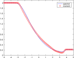
(a) $N=1$

(b) $N=2$

(c) $N=3$

(d) $N=4$

(e) $N=5$

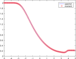
(f) $N=6$

Figure 5.1: Example 5.1: The densities at $t=4$ obtained by the moment method with $N=1,2,\cdots,6$ and 2000 cells. The solid line is the reference solution obtained by using the spectral method with 4000 cells. $\varepsilon=1$.

(a) $N=1$

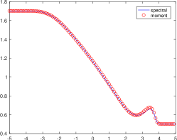
(b) $N=2$

(c) $N=3$

(d) $N=4$

(e) $N=5$

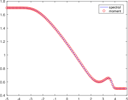
(f) $N=6$

Figure 5.2: Same as Fig. 5.1 except for the macroscopic velocity angles.

(a) $N=1$

(b) $N=2$

(c) $N=3$

(d) $N=4$

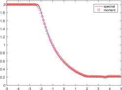
(e) $N=5$

(f) $N=6$

Figure 5.3: Same as Fig. 5.1 except for $\varepsilon=0.01$.

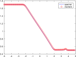
(a) $N=1$

(b) $N=2$

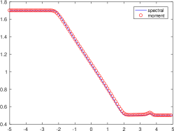
(c) $N=3$

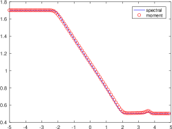
(d) $N=4$

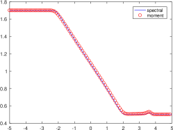
(e) $N=5$

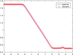
(f) $N=6$

Figure 5.4: Same as Fig. 5.3 except for the macroscopic velocity angles.

Example 5.2 (Shock wave).

The initial data of the second Riemann problem are

$$(\rho^{\varepsilon},\bar{\theta}^{\varepsilon})=\begin{cases}(1,1.5),&x<0,\\ (2,1.83),&x>0.\end{cases}$$

Figs. 5.5 and 5.6 give the densities $\rho^{\varepsilon}$ and macroscopic velocity angles $\bar{\theta}^{\varepsilon}$ at $t=4$ obtained by the moment method with $N=1,2,\cdots,6$, 2000 cells, and $\varepsilon=1$, where the solid line denotes the reference solution obtained by using the spectral method with 4000 cells. Figs. 5.7 and 5.8 display corresponding solutions for the case of $\varepsilon=0.01$. It is observed that a shock wave solution is generated and the solutions of moment method $(\rho^{\varepsilon},\bar{\theta}^{\varepsilon})$ do converge the shock profile as $\varepsilon$ becomes small, and the solutions of the moment system well agree with the reference when $N$ is larger than 1.

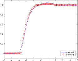
(a) $N=1$

(b) $N=2$

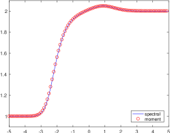
(c) $N=3$

(d) $N=4$

(e) $N=5$

(f) $N=6$

Figure 5.5: Example 5.2: The densities at $t=4$ obtained by the moment method with $N=1,2,\cdots,6$ and 2000 cells. The solid line is the reference solution obtained by using the spectral method with 4000 cells. $\varepsilon=1$.

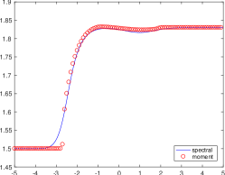
(a) $N=1$

(b) $N=2$

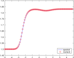
(c) $N=3$

(d) $N=4$

(e) $N=5$

(f) $N=6$

Figure 5.6: Same as Fig. 5.5 except for the macroscopic velocity angles.

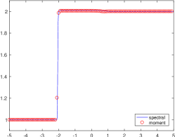
(a) $N=1$

(b) $N=2$

(c) $N=3$

(d) $N=4$

(e) $N=5$

(f) $N=6$

Figure 5.7: Same as Fig. 5.5 except for $\varepsilon=0.01$.

(a) $N=1$

(b) $N=2$

(c) $N=3$

(d) $N=4$

(e) $N=5$

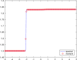
(f) $N=6$

Figure 5.8: Same as Fig. 5.7 except for the macroscopic velocity angles.

Example 5.3 (Contact discontinuity).

The initial data of the third Riemann problem are

$$(\rho^{\varepsilon},\bar{\theta}^{\varepsilon})=\begin{cases}(1,1),&x<0,\\ (1,-1),&x>0.\end{cases}$$

It is a contact discontinuity problem.

Figs. 5.9 and 5.10 show the densities $\rho^{\varepsilon}$ and macroscopic velocity angles $\bar{\theta}^{\varepsilon}$ at $t=4$ obtained by the moment method with $N=1,2,\cdots,6$, 4000 cells, and $\varepsilon=1$, where the solid line denotes the reference solution obtained by using the spectral method with 8000 cells. Figs. 5.11 and 5.12 display corresponding solutions for the case of $\varepsilon=0.01$. It is observed that the solutions of moment method $(\rho^{\varepsilon},\bar{\theta}^{\varepsilon})$ do converge the contact profile as $\varepsilon$ becomes small, and the solutions of the moment system agree with the reference when $N$ is larger than 3. When the $\varepsilon$ is smaller, the convergence rate of the moment method is faster, and for a fixed $\varepsilon$, the faster the $N$, the faster the convergence rate.

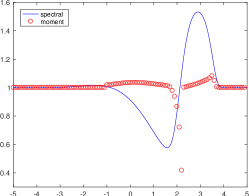
(a) $N=1$

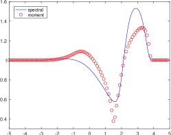
(b) $N=2$

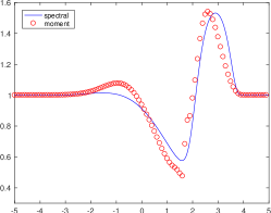
(c) $N=3$

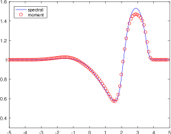
(d) $N=4$

(e) $N=5$

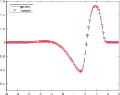
(f) $N=6$

Figure 5.9: Example 5.3: The densities at $t=4$ obtained by the moment method with $N=1,2,\cdots,6$ and 4000 cells. The solid line is the reference solution obtained by using the spectral method with 8000 cells. $\varepsilon=1$.

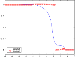
(a) $N=1$

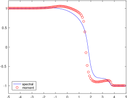
(b) $N=2$

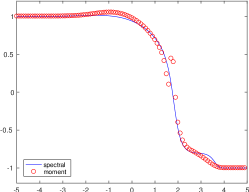
(c) $N=3$

(d) $N=4$

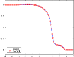
(e) $N=5$

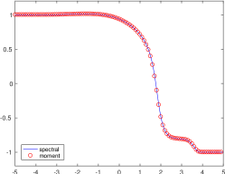
(f) $N=6$

Figure 5.10: Same as Fig. 5.9 except for the macroscopic velocity angles.

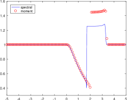
(a) $N=1$

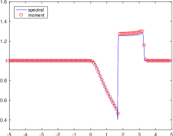
(b) $N=2$

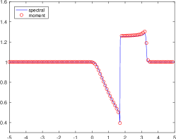
(c) $N=3$

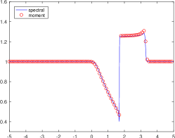
(d) $N=4$

(e) $N=5$

(f) $N=6$

Figure 5.11: Same as Fig. 5.9 except for $\varepsilon=0.01$.

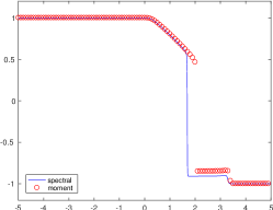
(a) $N=1$

(b) $N=2$

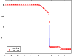
(c) $N=3$

(d) $N=4$

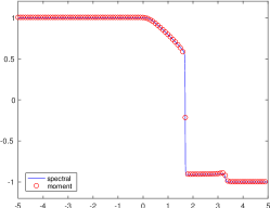
(e) $N=5$

(f) $N=6$

Figure 5.12: Same as Fig. 5.11 except for the macroscopic velocity angles.

Example 5.4 (Vortex formation).

The computational domain is chosen as the square area $[-5,5]\times[-5,5]$ with reflection boundary conditions, and is divided into a uniform square mesh $\{(x_{i},y_{j})|x_{i}=-5+ih,y_{j}=-5+jh,i,j=0,1,\cdots,n-1\}$. The initial data are taken as follows

$$f(0,x_{i},y_{j},\theta)=\dfrac{1}{2\pi},\ \ \bar{\theta}(0,x_{i},y_{j})=\begin{cases}0,&x<4.5,\\ \dfrac{\pi}{2},&\text{otherwise}.\end{cases}$$

After a transient period, the solution will converge to a steady state consisting of a vortex-type formation.

In numerical simulation, a perturbation is added to the initial velocity direction on the right boundary in order to ensure that the final steady state is counterclockwise rotation, and the solutions are output when the relative $\ell^{2}$ error of the density between two adjacent iterations is less than $1.5\times 10^{-3}$.

Figs. 5.13-5.15 show the densities and the velocities obtained by using the moment methods with $N=2,3,4$, $\varepsilon=1$, and the mesh of $n=20$, where 13 equally spaced contour lines are chosen from 0 to 2.4 with stepsize 0.2. Figs. 5.16-5.18 shows corresponding results for $n=50$. For the sake of comparison, Fig. 5.19 also gives the results obtained by using the spectral method with $n=25$. Fig. 5.20 shows the total mass $M(l)$ on the square $\Omega(l)$ and the relative $\ell^{2}$ errors of density, where

$$M(l)=\int_{\Omega(l)}\rho\mathrm{d}s,$$

and

$$\Omega(l)=\{(x,y)|\max\{\lvert x\rvert,\lvert y\rvert\}=l\},$$

and “N2n20” etc. in the legend represent “$N=2,n=20$” etc., while “specn20” denotes the spectral method with $n=20$. The distributions of $M(l)$ agree well with each other with some discrepancy near the boundary of the domain ($l\approx 5$). The discrepancies reduce as the number of moment and mesh cell increases. By observing the numerical error plots, it can be seen that with the increase of time step number, the errors are decreased, and the speed of convergence to the steady state solution becomes slow as the mesh number $n$ or the moment number $N$ is increasing.

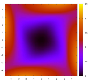
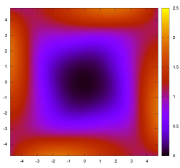
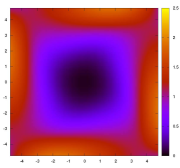
Figure 5.13: Example 5.4: The schlieren images of density obtained by using the moment method with $n=20$. From left to right: $N=2,3,4$.

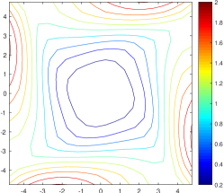
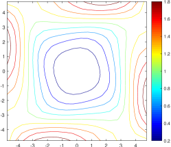
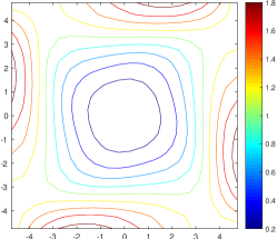
Figure 5.14: Same as Fig. 5.13 except for the density contours.

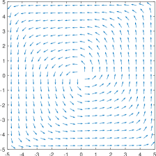
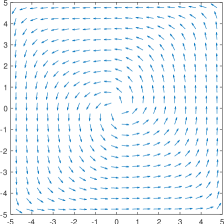
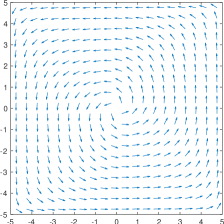
Figure 5.15: Same as Fig. 5.13 except for the arrow diagrams of velocity.

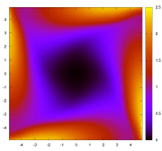
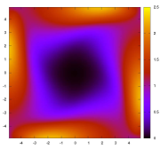
Figure 5.16: Same as Fig. 5.13 except for $n=50$.

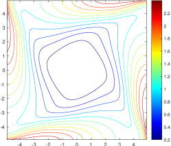
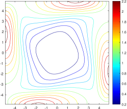
Figure 5.17: Same as Fig. 5.16 except for the density contours.

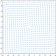
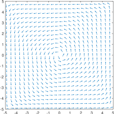
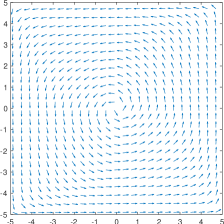
Figure 5.18: Same as Fig. 5.16 except for the arrow diagram of velocity.

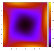
(a) Density

(b) Density

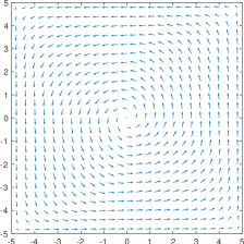
(c) Velocity

Figure 5.19: Same as Figs. 5.13-5.15 except for the spectral method with $n=25$.

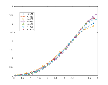
(a) Total mass $M(l)$

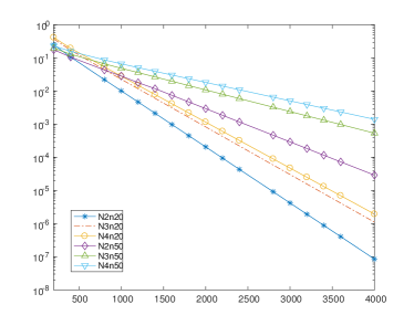
(b) Relative $\ell^{2}$ errors

Figure 5.20: Example 5.4: The total mass $M(l)$ on the square $\Omega(l)$ and the relative $\ell^{2}$ errors of density obtained by using moment methods.

6 Conclusions

The paper extended the model reduction method by the operator projection to a non-linear kinetic description of the Vicsek swarming model. First, a family of the complicate Grad type orthogonal functions depending on a parameter (angle of macroscopic velocity) were carefully studied in the regard of calculating their derivatives and projection of those derivatives and the product of velocity and basis and collision term. Next, building on those discussions and the operator projection, arbitrary order globally hyperbolic moment system of the kinetic description of the Vicsek swarming model was derived and their mathematical properties such as hyperbolicity, rotational invariance, mass-conservation and relationship between Grad type expansions in different parameter were also investigated. Finally, a semi-implicit numerical scheme was presented to solve a Cauchy problem of our hyperbolic moment system in order to verify the convergence behavior of the moment method. It was also compared to the spectral method for the kinetic equation. It was seen that the solutions of our hyperbolic moment system could converge to the solutions of the kinetic equation for the Vicsek swarming model as the order of the moment system increases, and the moment method could successfully capture key features such as shock wave, contact discontinuity, rarefaction wave, and vortex formation.

References

- [1] R. Bouffanais, Design and Control of Swarm Dynamics, Springer, 2016.
- [2] Z. Cai, Y. Fan, and R. Li, Globally hyperbolic regularization of Grad’s moment system in one dimensional space, Commun. Math. Sci., 11(2013), 547–571.
- [3] Z. Cai, Y. Fan, and R. Li, Globally hyperbolic regularization of Grad’s moment system, Comm. Pure Appl. Math., 67(2014), 464–518.
- [4] Z. Cai, Y. Fan, and R. Li, A framework on moment model reduction for kinetic equation, SIAM J. Appl. Math., 75(2014), 2001–2023.
- [5] Z. Cai and R. Li, Numerical regularized moment method of arbitrary order for Boltzmann-BGK equation, SIAM J. Sci. Comput., 32(2010), 2875–2907.
- [6] Z. Cai, R. Li, and Y. Wang, Numerical regularized moment method for high Mach number flow, Commun. Comput. Phys., 11(2012), 1415–1438.
- [7] J.A. Caizo, J. Carrillo, and J. Rosado, A well-posedness theory in measures for some kinetic models of collective motion, Math. Models Meth. Appl. Sci., 21(2011), 515–539.
- [8] C. Cercignani, The Boltzmann Equation and Its Applications, Springer, 1988.
- [9] S. Chapman and T.G. Cowling, The Mathematical Theory of Non-uniform Gases, 3rd ed., Cambridge Univ. Press, 1991.
- [10] P. Degond, J.G. Liu, S. Motsch, and V. Panferov, Hydrodynamic models of self-organized dynamics: derivation and existence theory, Meth. and Appl. Anal., 20(2013), 89–114.
- [11] P. Degond and S. Motsch, Continuum limit of self-driven particles with orientation interaction, Math. Models Meth. Appl. Sci., 18(2008), 1193–1215.
- [12] Y. Fan, J. Koellermeier, J. Li, R. Li, and M. Torrilhon, Model reduction of kinetic equations by operator projection, J. Stat. Phys., 162(2016), 457–486.
- [13] I.M. Gamba, J.R. Haack, and S. Motsch, Spectral method for a kinetic swarming model, J. Comput. Phys., 297(2015), 32–46.
- [14] I.M. Gamba and M.J. Kang, Global weak solutions for Kolmogorov-Vicsek type equations with orientational interactions, Arch. Rational Mech. Anal., 222(2015), 1–26.
- [15] H. Grad, On the kinetic theory of rarefied gases, Commun. Pure Appl. Math., 2(1949), 331–407.
- [16] H. Grad, Note on -dimensional Hermite polynomials, Commun. Pure Appl. Math., 2(1949), 325–330.
- [17] S.Y. Ha and E. Tadmor, From particle to kinetic and hydrodynamic descriptions of flocking, Kinet. Relat. Mod., 1(2008), 415–435.
- [18] J. Koellermeier and M. Torrilhon, Hyperbolic moment equations using quadrature based projection methods, AIP Conf. Proc., 1628(2014), 626–633.
- [19] J. Koellermeier, R. Schaerer, and M. Torrilhon, A framework for hyperbolic approximation of kinetic equations using quadrature-based projection methods, Kinet. Relat. Mod., 7(2014), 531–549.
- [20] Y.Y. Kuang and H.Z.Tang, Globally hyperbolic moment model of arbitrary order for one-dimensional special relativistic Boltzmann equation, preprint, arXiv: 1608.06555v2, 2016.
- [21] S. Rhebergen, O. Bokhove, and J. J. W. Van Der Vegt, Discontinuous Galerkin finite element methods for hyperbolic nonconservative partial differential equations, J. Comput. Phys., 227(2008), 1887–1922.