Graph Equivalence Classes for Spectral Projector-Based Graph Fourier Transforms

Abstract

We define and discuss the utility of two equivalence graph classes over which a spectral projector-based graph Fourier transform is equivalent: isomorphic equivalence classes and Jordan equivalence classes. Isomorphic equivalence classes show that the transform is equivalent up to a permutation on the node labels. Jordan equivalence classes permit identical transforms over graphs of nonidentical topologies and allow a basis-invariant characterization of total variation orderings of the spectral components. Methods to exploit these classes to reduce computation time of the transform as well as limitations are discussed.

I Introduction

Graph signal processing [1, 2] permits applications of digital signal processing concepts to increasingly larger networks. It is based on defining a shift filter, for example, the adjacency matrix in [1, 3, 4] to analyze undirected and directed graphs, or the graph Laplacian [2] that applies to undirected graph structures. The graph Fourier transform is defined through the eigendecomposition of this shift operator, see these references. Further developments have been considered in [5, 6, 7]. In particular, filter design [1, 5, 8] and sampling [9, 10, 11] can be applied to reduce the computational complexity of graph Fourier transforms.

With the objective of simplifying graph Fourier transforms for large network applications, this paper explores methods based on graph equivalence classes to reduce the computation time of the subspace projector-based graph Fourier transform proposed in [12]. This transform extends the graph signal processing framework proposed by [1, 3, 4] to consider spectral analysis over directed graphs with potentially non-diagonalizable (defective) adjacency matrices. The graph signal processing framework of [12] allows for a unique, unambiguous signal representation over defective adjacency matrices.

Consider a graph $\mathcal{G}=G(A)$ with adjacency matrix $A\in\mathbb{C}^{N\times N}$ with $k\leq N$ distinct eigenvalues and Jordan decomposition $A=VJV^{-1}$. The associated Jordan subspaces of $A$ are $\mathscr{J}_{ij}$, $i=1,\dots k$, $j=1,\dots,g_{i}$, where $g_{i}$ is the geometric multiplicity of eigenvalue $\lambda_{i}$, or the dimension of the kernel of $A-\lambda_{i}I$. The signal space $\mathcal{S}$ can be uniquely decomposed by the Jordan subspaces (see [13, 14] and Section II). For a graph signal $s\in\mathcal{S}$, the graph Fourier transform (GFT) of [12] is defined as

$$\mathcal{F}:\mathcal{S} \rightarrow\bigoplus_{i=1}^{k}\bigoplus_{j=1}^{g_{i}}\mathscr{J}_{ij}$$

$$s \rightarrow\left(\widehat{s}_{11},\dots,\widehat{s}_{1g_{1}},\dots,\widehat{s}_{k1},\dots,\widehat{s}_{kg_{k}}\right),$$ (1)

where $s_{ij}$ is the (oblique) projection of $s$ onto the Jordan subspace $J_{ij}$ parallel to $\mathcal{S}\backslash\mathscr{J}_{ij}$. That is, the Fourier transform of $s$, is the unique decomposition

$$s=\sum_{i=1}^{k}\sum_{j=1}^{g_{i}}\widehat{s}_{ij},\hskip 28.45274pt\widehat{s}_{ij}\in\mathscr{J}_{ij}.$$ (2)

The spectral components are the Jordan subspaces of the adjacency matrix with this formulation.

This paper presents graph equivalence classes where equal GFT projections by (1) are the equivalence relation. First, the transform (1) is invariant to node permutations, which we formalize with the concept of isomorphic equivalence classes. Furthermore, the GFT permits degrees of freedom in graph topologies, which we formalize by defining Jordan equivalence classes, a concept that allows graph Fourier transform computations over graphs of simpler topologies. A frequency-like ordering based on total variation of the spectral components is also presented to motivate low-pass, high-pass, and pass-band graph signals.

Section II provides the graph signal processing and linear algebra background for the graph Fourier transform (1). Isomorphic equivalence classes are defined in Section III, and Jordan equivalence classes are defined in Section IV. The Jordan equivalence classes influence the definition of total variation-based orderings of the Jordan subspaces, which is discussed in detail in Section V. Section VI illustrates Jordan equivalence classes and total variation orderings. Limitations of the method are discussed in Section VII.

II Background

This section reviews the concepts of graph signal processing and the GFT (1). Background on graphs signal processing, including definitions of graph signals and the graph shift, is described in greater detail in [1, 3, 4, 12]. For background on eigendecompositions, the reader is directed to in [13, 15, 16].

II-A Eigendecomposition

Consider matrix $A\in\mathbb{C}^{N\times N}$ with $k$ distinct eigenvalues $\lambda_{1},\dots,\lambda_{k}$, $k\leq N$. The algebraic multiplicity $a_{i}$ of $\lambda_{i}$ represents the corresponding exponent of the characteristic polynomial of $A$. Denote by $\mathrm{Ker}(A)$ the kernel or null space of matrix $A$. The geometric multiplicity $g_{i}$ of eigenvalue $\lambda_{i}$ equals the dimension of $\mathrm{Ker}\left(A-\lambda_{i}I\right)$, which is the eigenspace of $\lambda_{i}$ where $I$ is the $N\times N$ identity matrix. The generalized eigenspaces $\mathscr{G}_{i}$, $i=1,\dots,k$, of $A$ are defined as

$$\mathscr{G}_{i}=\mathrm{Ker}(A-\lambda_{i}I)^{m_{i}},$$ (3)

where $m_{i}$ is the index of eigenvalue $\lambda_{i}$. The generalized eigenspaces uniquely decompose $\mathbb{C}^{N}$ as the direct sum

$$\mathbb{C}^{N}=\bigoplus_{i=1}^{k}\mathscr{G}_{i}.$$ (4)

Jordan chains. Let $v_{1}\in\mathrm{Ker}(A-\lambda_{i}I)$, $v_{1}\neq 0$, be a proper eigenvector of $A$ that generates generalized eigenvectors by the recursion

$$Av_{p}=\lambda_{i}v_{p}+v_{p-1},\>\>p=2,\dots,r$$ (5)

where $r$ is the minimal positive integer such that $\left(A-\lambda_{i}I\right)^{r}v_{r}=0$ and $\left(A-\lambda_{i}I\right)^{r-1}v_{r}\neq 0$. A sequence of vectors $(v_{1},\dots,v_{r})$ that satisfy (5) is a Jordan chain of length $r$ [13]. The vectors in a Jordan chain are linearly independent and generate the Jordan subspace

$$\mathscr{J}=\mathrm{span}\left(v_{1},v_{2},\dots,v_{r}\right).$$ (6)

Denote by $\mathscr{J}_{ij}$ the $j$th Jordan subspace of $\lambda_{i}$ with dimension $r_{ij}$, $i=1,\dots,k$, $j=1,\dots,g_{i}$. The Jordan spaces are disjoint and uniquely decompose the generalized eigenspace $\mathscr{G}_{i}$ (3) of $\lambda_{i}$ as

$$\mathscr{G}_{i}=\bigoplus_{j=1}^{g_{i}}\mathscr{J}_{ij}.$$ (7)

The space $\mathbb{C}^{N}$ can be expressed as the unique decomposition of Jordan spaces

$$\mathbb{C}^{N}=\bigoplus_{i=1}^{k}\bigoplus_{j=1}^{g_{i}}\mathscr{J}_{ij}.$$ (8)

Jordan decomposition. Let $V_{ij}$ denote the $N\times r_{ij}$ matrix whose columns form a Jordan chain of eigenvalue $\lambda_{i}$ that spans Jordan subspace $\mathscr{J}_{ij}$. Then the eigenvector matrix $V$ of $A$ is

$$V=\begin{bmatrix}V_{11}\cdots V_{1g_{1}}&\cdots&V_{k1}\cdots V_{kg_{k}}\end{bmatrix},$$ (9)

where $k$ is the number of distinct eigenvalues. The columns of $V$ are a Jordan basis of $\mathbb{C}^{N}$. Then $A$ has block-diagonal Jordan normal form $J$ consisting of Jordan blocks

$$J(\lambda)=\begin{bmatrix}\lambda&1&\\ &\lambda&\ddots\\ &&\ddots&1\\ &&&\lambda\end{bmatrix}.$$ (10)

of size $r_{ij}$. The Jordan normal form $J$ of $A$ is unique up to a permutation of the Jordan blocks. The Jordan decomposition of $A$ is $A=VJV^{-1}$.

II-B Spectral Components

The spectral components of the Fourier transform (1) are expressed in terms of the eigenvector basis $v_{1},\dots,v_{N}$ and its dual basis $w_{1},\dots,w_{N}$ since the Jordan basis may not be orthogonal. Denote the basis and dual basis matrices by $V=[v_{1}\cdots v_{N}]$ and $W=[w_{1}\cdots,w_{N}]$. The dual basis matrix is the inverse Hermitian $W=V^{-H}$ [14, 17].

Consider the $j$th spectral component of $\lambda_{i}$

$$\mathscr{J}_{ij}=\mathrm{span}(v_{1},\cdots v_{r_{ij}}).$$ (11)

The projection matrix onto $\mathscr{J}_{ij}$ parallel to $\mathbb{C}^{N}\backslash\mathscr{J}_{ij}$ is

$$P_{ij}=V_{ij}W^{H}_{ij},$$ (12)

where

$$V_{ij}=[v_{1}\cdots v_{r_{ij}}]$$ (13)

is the corresponding submatrix of $V$ and $W^{H}_{ij}\in\mathbb{C}^{r_{ij}\times N}$ is the corresponding submatrix of $W$ partitioned as

$$W=[\cdots W_{i1}^{H}\cdots W_{ig_{i}}^{H}\cdots]^{T}.$$ (14)

As shown in [12], the projection of signal $s\in\mathbb{C}^{N}$ onto Jordan subspace $\mathscr{J}_{ij}$ can be written as

$$\widehat{s}_{ij} =\widetilde{s}_{1}v_{1}+\dots+\widetilde{s}_{r_{ij}}v_{r_{ij}}$$ (15)

$$=V_{ij}W^{H}_{ij}s.$$ (16)

The next sections show that invariance of the graph Fourier transform (1) is a useful equivalence relation on a set of graphs. Equivalence classes with respect to the GFT are explored in Sections III and IV.

III Isomorphic Equivalence Classes

This section demonstrates that the graph Fourier transform (1) is invariant up to a permutation of node labels and establishes sets of isomorphic graphs as equivalence classes with respect to invariance of the GFT (1). Two graphs $\mathcal{G}(A)$ and $\mathcal{G}(B)$ are isomorphic if their adjacency matrices are similar with respect to a permutation matrix $T$, or $B=TAT^{-1}$ [18]. The graphs have the same Jordan normal form and the same spectra. Also, if $V_{A}$ and $V_{B}$ are eigenvector matrices of $A$ and $B$, respectively, then $V_{B}=TV_{A}$. We prove that the set $\mathbf{G}_{A}^{I}$ of all graphs that are isomorphic to $\mathcal{G}(A)$ is an equivalence class over which the GFT is preserved. The next theorem shows that an appropriate permutation can be imposed on the graph signal and GFT to ensure invariance of the GFT over all graphs $\mathcal{G}\in\mathbf{G}_{A}^{I}$.

Theorem 1.

The graph Fourier transform of a signal $s$ is invariant to the choice of graph $\mathcal{G}\in\mathbf{G}_{A}^{I}$ up to a permutation on the graph signal and inverse permutation on the graph Fourier transform.

Proof:

For $\mathcal{G}(A),\mathcal{G}(B)\in\mathbf{G}_{A}^{I}$, there exists a permutation matrix $T$ such that $B=TAT^{-1}$. For eigenvector matrices $V_{A}$ and $V_{B}$ of $A$ and $B$, respectively, let $V_{A,ij}$ and $V_{B,ij}$ denote the $N\times r_{ij}$ submatrices of $V_{A}$ and $V_{B}$ whose columns span the $j$th Jordan subspaces $\mathscr{J}_{A,ij}$ and $\mathscr{J}_{B,ij}$ of the $i$th eigenvalue of $A$ and $B$, respectively. Let $W_{A}=V_{A}^{-H}$ and $W_{B}=V_{B}^{-H}$ denote the matrices whose columns form dual bases of $V_{A}$ and $V_{B}$. Since $V_{B}=TV_{A}$,

$$W_{B} =(TV_{A})^{-H}$$ (17)

$$=(V_{A}^{-1}T^{-1})^{H}$$ (18)

$$=T^{-H}V_{A}^{-H}$$ (19)

$$=TW_{A},$$ (20)

where $T^{-H}=T$ since $T$ is a permutation matrix. Thus,

$$W_{B}^{H}=W_{A}^{H}T^{H}=W_{A}^{H}T^{-1}.$$ (21)

Consider graph signal $s$. By (16), the signal projection onto $\mathscr{J}_{A,ij}$ is

$$\widehat{s}_{A,ij}=V_{A,ij}W_{A,ij}^{H}s.$$ (22)

Permit a permutation $\overline{s}=Ts$ on the graph signal. Then the projection of $\overline{s}$ onto $\mathscr{J}_{B,ij}$ is

$$\widehat{\overline{s}}_{B,ij} =TV_{A,ij}W_{A,ij}^{H}T^{-1}Ts$$ (23)

$$=TV_{A,ij}W_{A,ij}^{H}s$$ (24)

$$=T\widehat{s}_{A,ij}$$ (25)

by (22). Therefore, the graph Fourier transform (1) is invariant to a choice among isomorphic graphs up to a permutation on the graph signal and inverse permutation on the Fourier transform. ∎

Theorem 2.

Consider $A\in\mathbb{C}^{N\times N}$. Then the set $\mathbf{G}_{A}^{I}$ of graphs isomorphic to $\mathcal{G}(A)$ is an equivalence class with respect to the invariance of the GFT (1) up to a permutation of the graph signal and inverse permutation of the graph Fourier transform.

Theorem 1 establishes an invariance of the GFT over graphs that only differ up to a node labeling, and Theorem 2 follows.

The isomorphic equivalence of graphs is important since it signifies that the rows and columns of an adjacency matrix can be permuted to accelerate the eigendecomposition. For example, permutations of highly sparse adjacency matrices can convert an arbitrary matrix to nearly diagonal forms, such as with the Cuthill-McKee algorithm [19]. Optimizations for such matrices in this form are discussed in [16] and [20], for example. In the next section, the degrees of freedom in graph topology are explored to define another GFT equivalence class.

IV Jordan Equivalence Classes

Since the Jordan subspaces of defective adjacency matrices are nontrivial (i.e., they have dimension larger than one), a degree of freedom exists on the graph structure so that the graph Fourier transform of a signal is equal over multiple graphs of different topologies. This section defines Jordan equivalence classes of graph structures over which the GFT (1) is equal for a given graph signal. The section proves important properties of this equivalence class that are used to explore inexact methods and real-world applications in [21].

The intuition behind Jordan equivalence is presented in Section IV-A, and properties of Jordan equivalence are described in Section IV-B. Section IV-C compares isomorphic and Jordan equivalent graphs. Sections IV-D, IV-E, IV-F, and IV-G prove properties for Jordan equivalence classes when adjacency matrices have particular Jordan block structures.

IV-A Intuition

Consider Figure 1, which shows a basis $\{V\}=\{v_{1},v_{2},v_{3}\}$ of $\mathbb{R}^{3}$ such that $v_{2}$ and $v_{3}$ span a two-dimensional Jordan space $\mathscr{J}$ of adjacency matrix $A$ with Jordan decomposition $A=VJV^{-1}$. The resulting projection of a signal $s\in\mathbb{R}^{N}$ as in (16) is unique.

Figure 1: Projections $\widehat{s}_{1}$ and $\widehat{s}_{2}$ (shown in red) of a signal $s$ (shown in black) onto a nontrivial Jordan subspace (span of $v_{1}$ and $v_{2}$) and the span of $v_{3}$, respectively, in $\mathbb{R}^{3}$. The projection onto the nontrivial subspace is invariant to basis choices $\{v_{1},v_{2}\}$ (in blue) or $\{\widetilde{v}_{1},\widetilde{v}_{2}\}$ (in green).

Note that the definition of the two-dimensional Jordan subspace $\mathscr{J}$ in Figure 1 is not basis-dependent because any spanning set $\{w_{2},w_{3}\}$ could be chosen to define $\mathscr{J}$. This can be visualized by rotating $v_{2}$ and $v_{3}$ on the two-dimensional plane. Any choice $\{w_{2},w_{3}\}$ corresponds to a new basis $\widetilde{V}$. Note that $\widetilde{A}=\widetilde{V}J\widetilde{V}^{-1}$ does not equal $A=VJV^{-1}$ for all choices of $\{w_{2},w_{3}\}$; the underlying graph topologies may be different, or the edge weights may be different. Nevertheless, their spectral components (the Jordan subspaces) are identical, and, consequently, the spectral projections of a signal onto these components are identical; i.e., the GFT (1) is equivalent over graphs $\mathcal{G}(A)$ and $\mathcal{G}(\widetilde{A})$. This observation leads to the definition of Jordan equivalence classes which preserve the GFT (1) as well as the underlying structure captured by the Jordan normal form $J$ of $A$. These classes are formally defined in the next section.

IV-B Definition and Properties

This section defines the Jordan equivalence class of graphs, over which the graph Fourier transform (1) is invariant. We will show that certain Jordan equivalence classes allow the GFT computation to be simplified.

Consider graph $\mathcal{G}(A)$ where $A$ has a Jordan chain that spans Jordan subspace $\mathscr{J}_{ij}$ of dimension $r_{ij}>1$. Then (15), and consequently, (16), would hold for a non-Jordan basis of $\mathscr{J}_{ij}$; that is, a basis could be chosen to find spectral component $\widehat{s}_{ij}$ such that the basis vectors do not form a Jordan chain of $A$. This highlights that the Fourier transform (1) is characterized not by the Jordan basis of $A$ but by the set ${\mathbf{J}}_{A}=\{\mathscr{J}_{ij}\}_{ij}$ of Jordan subspaces spanned by the Jordan chains of $A$. Thus, graphs with topologies yielding the same Jordan subspace decomposition of the signal space have the same spectral components. Such graphs are termed Jordan equivalent with the following formal definition.

Definition 3 (Jordan Equivalent Graphs).

Consider graphs $\mathcal{G}(A)$ and $\mathcal{G}(B)$ with adjacency matrices $A,B\in\mathbb{C}^{N\times N}$. Then $\mathcal{G}(A)$ and $\mathcal{G}(B)$ are Jordan equivalent graphs if all of the following are true:

1. $\mathbf{J}_{A}=\mathbf{J}_{B}$; and

2. $J_{A}=J_{B}$ (with respect to a fixed permutation of Jordan blocks).

Let $\mathbf{G}_{A}^{J}$ denote the set of graphs that are Jordan equivalent to $\mathcal{G}(A)$. Definition 3 and (1) establish that $\mathbf{G}_{A}^{J}$ is an equivalence class.

Theorem 4.

For $A\in\mathbb{C}^{N\times N}$, the set $\mathbf{G}_{A}^{J}$ of all graphs that are Jordan equivalent to $\mathcal{G}(A)$ is an equivalence class with respect to invariance of the GFT (1).

Jordan equivalent graphs have adjacency matrices with identical Jordan subspaces and identical Jordan normal forms. This implies equivalence of graph spectra, proven in Theorem 5 below.

Theorem 5.

Denote by $\Lambda_{A}$ and $\Lambda_{B}$ the sets of eigenvalues of $A$ and $B$, respectively. Let $\mathcal{G}(A),\mathcal{G}(B)\in\mathbf{G}_{A}^{J}$. Then $\Lambda_{A}=\Lambda_{B}$; that is, $\mathcal{G}(A)$ and $\mathcal{G}(B)$ are cospectral.

Proof:

Since $\mathcal{G}(A)$ and $\mathcal{G}(B)$ are Jordan equivalent, their Jordan forms are equal, so their spectra (the unique elements on the diagonal of the Jordan form) are equal. ∎

Once a Jordan decomposition for an adjacency matrix is found, it is useful to characterize other graphs in the same Jordan equivalence class. To this end, Theorem 6 presents a transformation that preserves the Jordan equivalence class of a graph.

Theorem 6.

Consider $A,B\in\mathbb{C}^{N\times N}$ with Jordan decompositions $A=VJV^{-1}$ and $B=XJX^{-1}$ and eigenvector matrices $V=[V_{ij}]$ and $X=[X_{ij}]$, respectively. Then, $\mathcal{G}(B)\in\mathbf{G}_{A}^{J}$ if and only if $B$ has eigenvector matrix $X=VY$ for block diagonal $Y$ with invertible submatrices $Y_{ij}\in\mathbb{C}^{r_{ij}\times r_{ij}}$, $i=1,\dots,k$, $j=1,\dots,g_{i}$.

Proof:

The Jordan normal forms of $A$ and $B$ are equal. By Definition 3, it remains to show $\mathbf{J}_{A}=\mathbf{J}_{B}$ so that $\mathcal{G}(B)\in\mathbf{G}_{A}^{J}$. The identity $\mathbf{J}_{A}=\mathbf{J}_{B}$ must be true when $\mathrm{span}\{V_{ij}\}=\mathrm{span}\{X_{ij}\}=\mathscr{J}_{ij}$, which implies that $X_{ij}$ represents an invertible linear transformation of the columns of $V_{ij}$. Thus, $X_{ij}=V_{ij}Y_{ij}$, where $Y_{ij}$ is invertible. Defining $Y=\mathrm{diag}(Y_{11},\dots,Y_{ij},\dots,Y_{k,g_{k}})$ yields $X=VY$. ∎

IV-C Jordan Equivalent Graphs vs. Isomorphic Graphs

This section shows that isomorphic graphs do not imply Jordan equivalence, and vice versa. First it is shown that isomorphic graphs have isomorphic Jordan subspaces.

Lemma 7.

Consider graphs $\mathcal{G}(A),\mathcal{G}(B)\in\mathbf{G}_{A}^{I}$ so that $B=TAT^{-1}$ for a permutation matrix $T$. Denote by $\mathbf{J}_{A}$ and $\mathbf{J}_{B}$ the sets of Jordan subspaces for $A$ and $B$, respectively. If $\{v_{1},\dots,v_{r}\}$ is a basis of $\mathscr{J}_{A}\in\mathbf{J}_{A}$, then there exists $\mathscr{J}_{B}\in\mathbf{J}_{B}$ with basis $\{x_{1},\dots,x_{r}\}$ such that $[x_{1}\cdots x_{r}]=T[v_{1}\cdots v_{r}]$; i.e., $A$ and $B$ have isomorphic Jordan subspaces.

Proof:

Consider $A$ with Jordan decomposition $A=VJV^{-1}$. Since $B=TAT^{-1}$, it follows that

$$B =TVJV^{-1}T^{-1}$$ (26)

$$=XJX^{-1}$$ (27)

where $X=TV$ represents an eigenvector matrix of $B$ that is a permutation of the rows of $V$. (It is clear that the Jordan forms of $A$ and $B$ are equivalent.) Let columns $v_{1},\dots,v_{r}$ of $V$ denote a Jordan chain of $A$ that spans Jordan subspace $\mathscr{J}_{A}$. The corresponding columns in $X$ are $x_{1},\dots,x_{r}$ and $\mathrm{span}(x_{1},\dots,x_{r})=\mathscr{J}_{B}$. Since $[x_{1}\ \cdots\ x_{r}]=T[v_{1}\ \cdots\ v_{r}]$, $\mathscr{J}_{A}$ and $\mathscr{J}_{B}$ are isomorphic subspaces [13]. ∎

Theorem 8.

A graph isomorphism does not imply Jordan equivalence.

Proof:

Consider $\mathcal{G}(A),\mathcal{G}(B)\in\mathbf{G}_{A}^{I}$ and $B=TAT^{-1}$ for permutation matrix $T$. By (27), $J_{A}=J_{B}$. To show $\mathcal{G}(A),\mathcal{G}(B)\in\mathbf{G}_{A}^{J}$, it remains to check whether $\mathbf{J}_{A}=\mathbf{J}_{B}$.

By Lemma 7, for any $\mathscr{J}_{A}\in\mathbf{J}_{A}$, there exists $\mathscr{J}_{B}\in\mathbf{J}_{B}$ that is isomorphic to $\mathscr{J}_{A}$. That is, if $v_{1},\dots,v_{r}$ and $x_{1},\dots,x_{r}$ are bases of $\mathscr{J}_{A}$ and $\mathscr{J}_{B}$, respectively, then $[x_{1}\cdots x_{r}]=T[v_{1}\cdots v_{r}]$. Checking $\mathscr{J}_{A}=\mathscr{J}_{B}$ is equivalent to checking

$$\alpha_{1}v_{1}+\dots+\alpha_{r}v_{r} =\beta_{1}x_{1}+\dots+\beta_{r}x_{r}$$ (28)

$$=\beta_{1}Tv_{1}+\dots+\beta_{r}Tv_{r}$$ (29)

for some coefficients $\alpha_{i}$ and $\beta_{i}$, $i=1,\dots,r$. However, (29) does not always hold. Consider matrices $A$ and $B$

$$A=\begin{bmatrix}2&0&-1\\ 0&2&-1\\ 0&0&1\end{bmatrix},B=\begin{bmatrix}1&0&0\\ -1&2&0\\ -1&0&2\end{bmatrix}.$$ (30)

These matrices are similar with respect to a permutation matrix and thus correspond to isomorphic graphs. Their Jordan normal forms are both

$$J=\begin{bmatrix}1&0&0\\ 0&2&0\\ 0&0&2\end{bmatrix}$$ (31)

with possible eigenvector matrices $V_{A}$ and $V_{B}$ given by

$$V_{A}=\begin{bmatrix}1&1&0\\ 1&0&1\\ 1&0&0\end{bmatrix},V_{B}=\begin{bmatrix}1&0&0\\ 1&1&0\\ 1&0&1\end{bmatrix}.$$ (32)

Equation (32) shows that $A$ and $B$ both have Jordan subspaces $\mathscr{J}_{1}=\mathrm{span}([1\ 1\ 1]^{T})$ for $\lambda_{1}=1$ and $\mathscr{J}_{21}=\mathrm{span}([0\ 1\ 0]^{T})$ for one Jordan subspace of $\lambda_{2}=2$. However, the remaining Jordan subspace is $\mathrm{span}([1\ 0\ 0]^{T})$ for $A$ but $\mathrm{span}([0\ 0\ 1]^{T})$ for $B$, so (29) fails. Thus, $\mathcal{G}(A)$ and $\mathcal{G}(B)$ are not Jordan equivalent. ∎

The next theorem shows that Jordan equivalent graphs may not be isomorphic.

Theorem 9.

Jordan equivalence does not imply the existence of a graph isomorphism.

Proof:

A counterexample is provided. The top two graphs in Figure 2 correspond to 0/1 adjacency matrices with a single Jordan subspace $\mathscr{J}=\mathbb{C}^{N}$ and eigenvalue $0$; therefore, they are Jordan equivalent. On the other hand, they are not isomorphic since the graph on the right has more edges then the graph on the left. ∎

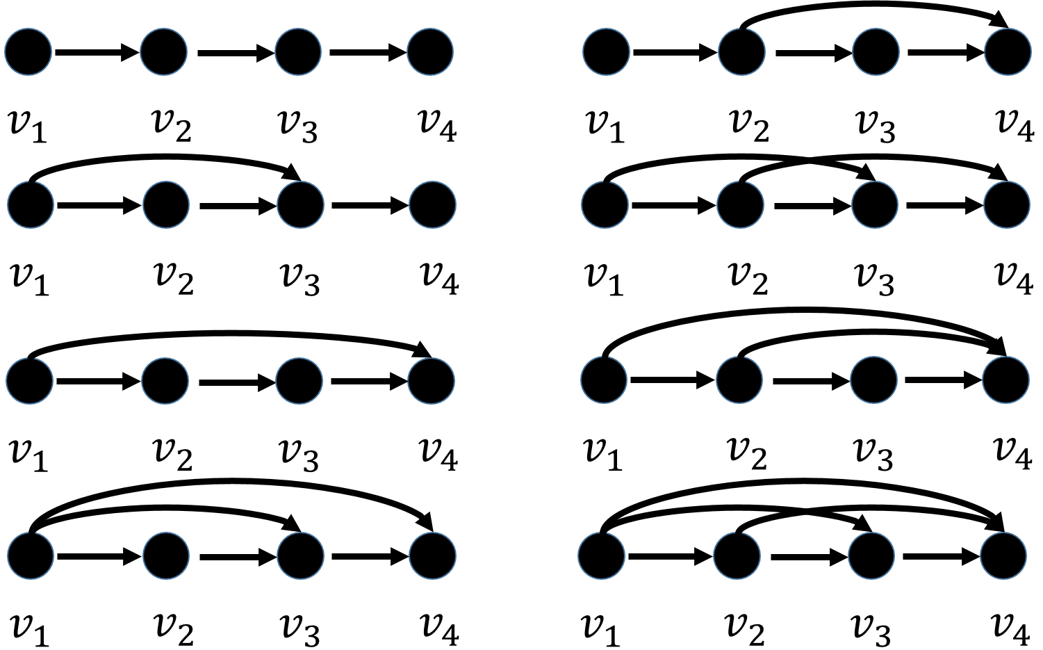
Figure 2: Jordan equivalent graph structures with unicellular adjacency matrices.

Theorem 8 shows that changing the graph node labels may change the Jordan subspaces and the Jordan equivalence class of the graph, while Theorem 9 shows that a Jordan equivalence class may include graphs with different topologies. Thus, graph isomorphism and Jordan equivalence are not identical concepts. Nevertheless, the isomorphic and Jordan equivalence classes both imply invariance of the graph Fourier transform with respect to equivalence relations as stated in Theorems 1 and 4.

The next theorem establishes an isomorphism between Jordan equivalence classes.

Theorem 10.

If $A,B\in\mathbb{C}^{N\times N}$ and $\mathcal{G}(A)$ and $\mathcal{G}(B)$ are isomorphic, then their respective Jordan equivalence classes $\mathbf{G}^{J}_{A}$ and $\mathbf{G}^{J}_{B}$ are isomorphic; i.e., any graph $\mathcal{G}(A^{\prime})\in\mathbf{G}_{A}^{J}$ is isomorphic to a graph $\mathcal{G}(B^{\prime})\in\mathbf{G}_{B}^{J}$.

Proof:

Let $\mathcal{G}(A)$ and $\mathcal{G}(B)$ be isomorphic by permutation matrix $T$ such that $B=TAT^{-1}$. Consider $\mathcal{G}(A^{\prime})\in\mathbf{G}_{A}^{J}$, which implies that Jordan normal forms $J_{A^{\prime}}=J_{A}$ and sets of Jordan subspaces $\mathbf{J}_{A^{\prime}}=\mathbf{J}_{A}$ by Definition 3. Denote by $A^{\prime}=V_{A^{\prime}}J_{A^{\prime}}V_{A^{\prime}}$ the Jordan decomposition of $A^{\prime}$. Define $B^{\prime}=TA^{\prime}T^{-1}$. It suffices to show $\mathcal{G}(B^{\prime})\in\mathbf{G}_{B}^{J}$. First simplify:

$$B^{\prime} =TA^{\prime}T^{-1}$$ (33)

$$=TV_{A^{\prime}}J_{A^{\prime}}V_{A^{\prime}}^{-1}T^{-1}$$ (34)

$$=TV_{A^{\prime}}J_{A}V_{A^{\prime}}^{-1}T^{-1}\hskip 14.22636pt\text{(since $\mathcal{G}(A^{\prime})\in\mathbf{G}_{A}^{J}$)}$$ (35)

$$=TV_{A^{\prime}}J_{B}V_{A^{\prime}}^{-1}T^{-1}\hskip 14.22636pt\text{(since $\mathcal{G}(A)\in\mathbf{G}_{B}^{I}$)}.$$ (36)

From (36), it follows that $J_{B^{\prime}}=J_{B}$. It remains to show that $\mathbf{J}_{B^{\prime}}=\mathbf{J}_{B}$. Choose arbitrary Jordan subspace $\mathscr{J}_{A,ij}=\mathrm{span}\{V_{A,ij}\}$ of $A$. Then $\mathscr{J}_{A^{\prime},ij}=\mathrm{span}\{V_{A^{\prime},ij}\}=\mathscr{J}_{A,ij}$ since $\mathcal{G}(A^{\prime})\in\mathbf{G}_{A}^{J}$. Then the $j$th Jordan subspace of eigenvalue $\lambda_{i}$ for $B$ is

$$\mathscr{J}_{B,ij} =\mathrm{span}\{TV_{A,ij}\}$$ (37)

$$=T\mathrm{span}\{V_{A,ij}\}.$$ (38)

For the $j$th Jordan subspace of eigenvalue $\lambda_{i}$ for $B^{\prime}$, it follows from (36) that

$$\mathscr{J}_{B^{\prime},ij} =\mathrm{span}\{TV_{A^{\prime},ij}\}$$ (39)

$$=T\mathrm{span}\{V_{A^{\prime},ij}\}$$ (40)

$$=T\mathrm{span}\{V_{A,ij}\}\hskip 28.45274pt\text{(since $\mathcal{G}(A^{\prime})\in\mathbf{G}_{A}^{J}$)}$$ (41)

$$=\mathscr{J}_{B,ij}.\hskip 56.9055pt\text{(by~{}\eqref{eq:thm:jordanequiv_inter})}$$ (42)

Since (42) holds for all $i$ and $j$, the sets of Jordan subspaces $\mathbf{J}_{B^{\prime}}=\mathbf{J}_{B}$. Therefore, $\mathcal{G}(B^{\prime})$ and $\mathcal{G}(B)$ are Jordan equivalent, which proves the theorem. ∎

Theorem 10 shows that the Jordan equivalence classes of two isomorphic graphs are also isomorphic. This result permits an frequency ordering on the spectral components of a matrix $A$ that is invariant to both the choice of graph in $\mathbf{G}_{A}^{J}$ and the choice of node labels, as demonstrated in Section V.

Relation to matrices with the same set of invariant subspaces. Let $\mathbf{G}_{A}^{\mathrm{Inv}}$ denote the set of all matrices with the same set of invariant subspaces of $A$; i.e., $\mathcal{G}(B)\in\mathbf{G}_{A}^{\mathrm{Inv}}$ if and only if $\mathrm{Inv}(A)=\mathrm{Inv}(B)$. The next theorem shows that $\mathbf{G}_{A}^{\mathrm{Inv}}$ is a proper subset of the Jordan equivalence class $\mathbf{G}_{A}^{J}$ of $A$.

Theorem 11.

For $A\in\mathbb{C}^{N\times N}$, $\mathbf{G}_{A}^{\mathrm{Inv}}\subset\mathbf{G}_{A}^{J}$.

Proof:

If $\mathcal{G}(B)\in\mathbf{G}_{A}^{\mathrm{Inv}}$, then the set of Jordan subspaces are equal, or $\mathbf{J}_{A}=\mathbf{J}_{B}$. ∎

Theorem 11 sets the results of this chapter apart from analyses such as those in Chapter 10 of [15], which describes structures for matrices with the same invariant spaces, and [22], which describes the eigendecomposition of the discrete Fourier transform matrix in terms of projections onto invariant spaces. The Jordan equivalence class relaxes the assumption that all invariant subspaces of two adjacency matrices must be equal. This translates to more degrees of freedom in the graph topology. The following sections present results for adjacency matrices with diagonal Jordan forms, one Jordan block, and multiple Jordan blocks.

IV-D Diagonalizable Matrices

If the canonical Jordan form $J$ of $A$ is diagonal ($A$ is diagonalizable), then there are no Jordan chains and the set of Jordan subspaces $\mathbf{J}_{A}=\{\mathscr{J}_{p}\}_{p=1}^{N}$ where $\mathscr{J}_{p}=\mathrm{span}(v_{p})$ and $v_{p}$ is the $p$th eigenvector of $A$. Graphs with diagonalizable adjacency matrices include undirected graphs, directed cycles, and other digraphs with normal adjacency matrices such as normally regular digraphs [23]. A graph with a diagonalizable adjacency matrix is Jordan equivalent only to itself, as proven next.

Theorem 12.

A graph $\mathcal{G}(A)$ with diagonalizable adjacency matrix $A\in\mathbb{C}^{N\times N}$ belongs to a Jordan equivalence class of size one.

Proof:

Since the Jordan subspaces of a diagonalizable matrix are one-dimensional, the possible choices of Jordan basis are limited to nonzero scalar multiples of the eigenvectors. Then, given eigenvector matrix $V$ of $A$, all possible eigenvector matrices of $A$ are given by $X=VU$, where $U$ is a diagonal matrix with nonzero diagonal entries. Let $B=XJX^{-1}$, where $J$ is the diagonal canonical Jordan form of $A$. Since $U$ and $J$ are both diagonal, they commute, yielding

$$B =XJX^{-1}$$ (43)

$$=VUJU^{-1}V^{-1}$$ (44)

$$=VJUU^{-1}V^{-1}$$ (45)

$$=VJV^{-1}$$ (46)

$$=A.$$ (47)

Thus, a graph with a diagonalizable adjacency matrix is the one and only element in its Jordan equivalence class. ∎

When a matrix has nondefective but repeated eigenvalues, there are infinitely many choices of eigenvectors [16]. An illustrative example is the identity matrix, which has a single eigenvalue but is diagonalizable. Since it has infinitely many choices of eigenvectors, the identity matrix corresponds to infinitely many Jordan equivalence classes. By Theorem 12, each of these equivalence classes have size one. This observation highlights that the definition of a Jordan equivalence class requires a choice of basis.

IV-E One Jordan Block

Consider matrix $A$ with Jordan decomposition $A=VJV^{-1}$ where $J$ is a single Jordan block and $V=[v_{1}\cdots v_{N}]$ is an eigenvector matrix. Then $A$ is a representation of a unicellular transformation $T:\mathbb{C}^{N}\rightarrow\mathbb{C}^{N}$ with respect to Jordan basis $v_{1},\dots v_{N}$ (see [15, Section 2.5]). In this case the set of Jordan subspaces has one element $\mathscr{J}=\mathbb{C}^{N}$. Properties of unicellular Jordan equivalence classes are demonstrated next.

Theorem 13.

Let $\mathcal{G}(A)$ be an element of the unicellular Jordan equivalence class $\mathbf{G}_{A}^{J}$. Then all graph filters $H\in\mathbf{G}_{A}^{J}$ are all-pass.

Proof:

Since $A$ is unicellular, it has a single Jordan chain $v_{1},\dots,v_{N}$ of length $N$. Consider a graph signal $s$ over graph $\mathcal{G}(A)$, and let $\widetilde{s}$ represent the coordinate vector of $s$ in terms of the basis $\{v_{i}\}_{i=1}^{N}$. Then the spectral decomposition of signal $s$ is given by

$$s=\widetilde{s}_{1}v_{1}+\cdots\widetilde{s}_{N}v_{N}=\widehat{s};$$ (48)

that is, the unique projection of $s$ onto the spectral component $\mathscr{J}=\mathbb{C}^{N}$ is itself. Therefore, $\mathcal{G}(A)$ acts as an all-pass filter. Moreover, (48) holds for all graphs in Jordan equivalence class $\mathbf{G}_{A}^{J}$. ∎

In addition to the all-pass property of unicellular graph filters, unicellular isomorphic graphs are also Jordan equivalent, as proven next.

Theorem 14.

Let $\mathcal{G}(A),\mathcal{G}(B)\in\mathbf{G}_{A}^{I}$ where $A$ is a unicellular matrix. Then $\mathcal{G}(A),\mathcal{G}(B)\in\mathbf{G}_{A}^{J}$.

Proof:

Since $\mathcal{G}(A)$ and $\mathcal{G}(B)$ are isomorphic, Jordan normal forms $J_{A}=J_{B}$. Therefore, $B$ is also unicellular, so $\mathbf{J}_{A}=\mathbf{J}_{B}=\{\mathbb{C}^{N}\}$. By Definition 3, $\mathcal{G}(A),\mathcal{G}(B)\in\mathbf{G}_{A}^{J}$. ∎

The dual basis of $V$ can also be used to construct graphs in the Jordan equivalence class of unicellular $A$.

Theorem 15.

Denote by $V$ an eigenvector matrix of unicellular $A\in\mathbb{C}^{N\times N}$ and $W=V^{-H}$ is the dual basis. Consider decompositions $A=VJV^{-1}$ and $A_{W}=WJW^{-1}$. Then $\mathcal{G}(A_{W})\in\mathbf{G}_{A}^{J}$.

Proof:

Matrices $A$ and $A_{W}$ have the same Jordan normal form by definition. Since there is only one Jordan block, both matrices have a single Jordan subspace $\mathbb{C}^{N}$. By Definition 3, $\mathcal{G}(A_{W})$ and $\mathcal{G}(A)$ are Jordan equivalent. ∎

The next theorem characterizes the special case of graphs in the Jordan equivalence class that contains $\mathcal{G}(J)$ with adjacency matrix equal to Jordan block $J=J(\lambda)$.

Theorem 16.

Denote by $J=J(\lambda)$ is the $N\times N$ Jordan block (10) for eigenvalue $\lambda$. Then $\mathcal{G}(A)\in\mathbf{G}_{J}^{J}$ if $A\in\mathbb{C}^{N\times N}$ is upper triangular with diagonal entries $\lambda$ and nonzero entries on the first off-diagonal.

Proof:

Consider upper triangular matrix $A=[a_{ij}]$ with diagonal entries $a_{11}=\cdots=a_{NN}$ and nonzero elements on the first off-diagonal. By [15, Example 10.2.1], $A$ has the same invariant subspaces as $J=J(\lambda)$, which implies $\mathbf{J}_{J}=\mathbf{J}_{A}=\{\mathbb{C}^{N}\}$. Therefore, the Jordan normal form of $A$ is the Jordan block $J_{A}=J(a_{11})$. Restrict the diagonal entries of $A$ to $\lambda$ so $J_{A}=J$. Then, $\mathcal{G}(J),\mathcal{G}(A)\in\mathbf{G}_{J}^{J}$ by Definition (3). ∎

Figure 2 shows graph structures that are in the same unicellular Jordan equivalence class by Theorem 16. In addition, the theorem implies that it is sufficient to determine the GFT of unicellular $A$ by replacing $\mathcal{G}(A)\in\mathbf{G}_{J}^{J}$ with $\mathcal{G}(J)$, where $J$ is a single $N\times N$ Jordan block. That is, without loss of generality, $\mathcal{G}(A)$ can be replaced with a directed chain graph with possible self-edges and the eigenvector matrix $V=I$ chosen to compute the GFT of a graph signal.

Remark on invariant spaces. Example 10.2.1 of [15] shows that a matrix $A\in\mathbb{C}^{N\times N}$ having upper triangular entries with constant diagonal entries $a$ and nonzero entries on the first off-diagonal is both necessary and sufficient for $A$ to have the same invariant subspaces as $N\times N$ Jordan block $J=J(\lambda)$ (i.e., $\mathrm{Inv}(J)=\mathrm{Inv}(A)$, where $\mathrm{Inv}(\cdot)$ represents the set of invariant spaces of a matrix). If $a=\lambda$, Definition 3 can be applied, which yields $\mathcal{G}(A)\in\mathbf{G}_{J}^{J}$.

On the other hand, consider a unicellular matrix $B$ such that its eigenvector is not in the span of a canonical vector, e.g.,

$$B=\begin{bmatrix}\frac{1}{2}&-\frac{1}{2}&\frac{1}{2}&\frac{1}{2}\\ \frac{1}{2}&-\frac{1}{2}&-\frac{1}{2}&-\frac{1}{2}\\ 0&0&\frac{1}{2}&-\frac{1}{2}\\ 0&0&\frac{1}{2}&-\frac{1}{2}\end{bmatrix}$$ (49)

with Jordan normal form $J(0)$. Since the span of the eigenvectors of $J(0)$ and $B$ are not identical, $\mathrm{Inv}(J(0))\neq\mathrm{Inv}(B)$. However, by Definition 3, $\mathcal{G}(B)$ is in the same class of unicellular Jordan equivalent graphs as those of Figure 2, i.e., $\mathcal{G}(B)\in\mathbf{G}_{J}^{J}$. In other words, for matrices $A$ and $B$ with the same Jordan normal forms ($J_{A}=J_{B}$), Jordan equivalence, i.e., $\mathbf{J}_{A}=\mathbf{J}_{B}$, is a more general condition than $\mathrm{Inv}(A)=\mathrm{Inv}(B)$. This illustrates that graphs having adjacency matrices with equal Jordan normal forms and the same sets of invariant spaces form a proper subset of a Jordan equivalence class, as shown above in Theorem 11.

Remark on topology. Note that replacing each nonzero element of (49) with a unit entry results in a matrix that is not unicellular. Therefore, its corresponding graph is not in a unicellular Jordan equivalence class. This observation demonstrates that topology may not determine the Jordan equivalence class of a graph.

IV-F Two Jordan Blocks

Consider $N\times N$ matrix $A$ with Jordan normal form consisting of two Jordan subspaces $\mathscr{J}_{1}=\mathrm{span}(v_{1},\dots,v_{r_{1}})$ and $\mathscr{J}_{2}=\mathrm{span}(v_{r_{1}+1},\dots,v_{r_{2}})$ of dimensions $r_{1}>1$ and $r_{2}=N-r_{1}$ and corresponding eigenvalues $\lambda_{1}$ and $\lambda_{2}$, respectively. The spectral decomposition of signal $s$ over $\mathcal{G}(A)$ yields

$$s =\underbrace{\widetilde{s}_{1}v_{1}+\cdots+\widetilde{s}_{r_{1}}v_{r_{1}}}_{\widehat{s}_{1}}+\underbrace{\widetilde{s}_{r_{1}+1}v_{r_{1}+1}+\cdots+\widetilde{s}_{N}v_{N}}_{\widehat{s}_{2}}$$ (50)

$$=\widehat{s}_{1}+\widehat{s}_{2}.$$ (51)

Spectral components $\widehat{s}_{1}$ and $\widehat{s}_{2}$ are the unique projections of $s$ onto the respective Jordan subspaces. By Example 6.5.4 in [13], a Jordan basis matrix $X$ can be chosen for $A=VJV^{-1}$ such that $X=VU$, where $U$ commutes with $J$ and has a particular form as follows.

If $\lambda_{1}\neq\lambda_{2}$, then $U=\mathrm{diag}(U_{1},U_{2})$, where $U_{i}$, $i=1,2$, is an $r_{i}\times r_{i}$ upper triangular Toeplitz matrix; otherwise, $U$ has form

$$U=\mathrm{diag}(U_{1},U_{2})+\begin{bmatrix}\underline{0}&U_{12}\\ U_{21}&\underline{0}\end{bmatrix}$$ (52)

where $U_{i}$ is an $r_{i}\times r_{i}$ upper triangular Toeplitz matrix and $U_{12}$ and $U_{21}$ are extended upper triangular Toeplitz matrices as in Theorem 12.4.1 in [13]. Thus, all Jordan bases of $A$ can be obtained by transforming eigenvector matrix $V$ as $X=VU$.

A corresponding theorem to Theorem 16 is presented to characterize Jordan equivalent classes when the Jordan form consists of two Jordan blocks. The reader is directed to Sections 10.2 and 10.3 in [15] for more details. The following definitions are needed. Denote $p\times p$ upper triangular Toeplitz matrices $T_{r_{2}}\left(b_{1},\dots,b_{r_{2}}\right)$ of form

$$T_{p}\left(b_{1},\dots,b_{p}\right)=\begin{bmatrix}b_{1}&b_{2}&\cdots&b_{p-1}&b_{p}\\ 0&b_{1}&\ddots&b_{p-2}&b_{p-1}\\ \vdots&\vdots&\ddots&\ddots&\vdots\\ 0&0&\cdots&b_{1}&b_{2}\\ 0&0&\cdots&0&b_{1}\\ \end{bmatrix},$$ (53)

and define $q\times q$ upper triangular matrix for some $q>p$

$$R_{q}\left(b_{1},\dots,b_{p};F\right)=$$

$$\begin{bmatrix}b_{1}&\cdots&b_{p}&f_{11}&f_{12}&\cdots f_{1,q-p-1}&f_{1,q-p}\\ 0&b_{1}&\cdots&b_{p}&f_{22}&\cdots f_{2,q-p-1}&f_{2,q-p}\\ \vdots&\vdots&\ddots&&\ddots&\vdots&\vdots\\ 0&0&&&\cdots&b_{p}&f_{q-p,q-p}\\ 0&0&&&\cdots&b_{p-1}&b_{p}\\ \vdots&\vdots&&&\vdots&\vdots&\vdots\\ 0&0&\cdots&&0&b_{1}&b_{2}\\ 0&0&\cdots&&0&0&b_{1}\\ \end{bmatrix}$$ (54)

where $F=[f_{ij}]$ is a $(q-p)\times(q-p)$ upper triangular matrix and $b_{i}\in\mathbb{C}$, $i=1,\dots,p$. The theorems are presented below.

Theorem 17.

Consider $A=\mathrm{diag}(A_{1},A_{2})$ where each matrix $A_{i}$, $i=1,2$, is upper triangular with diagonal elements $\lambda_{i}$ and nonzero elements on the first off-diagonal. Let $\lambda_{1}\neq\lambda_{2}$. Then $\mathcal{G}(A)$ is Jordan equivalent to the graph with adjacency matrix $J=\mathrm{diag}(J_{r_{1}}(\lambda_{1}),J_{r_{2}}(\lambda_{2}))$ where $J_{r_{i}}(\lambda_{i})$ is the $r_{i}\times r_{i}$ Jordan block for eigenvalue $\lambda_{i}$.

Proof:

By Theorem 16, $\mathcal{G}(A_{i})$ and $\mathcal{G}(J_{r_{i}}(\lambda_{i}))$ are Jordan equivalent for $i=1,2$ and $A_{i}$ upper triangular with nonzero elements on the first off-diagonal. Therefore, the Jordan normal forms of $J$ and $A$ are the same. Moreover, the set of irreducible subspaces of $J$ is the union of the irreducible subspaces of $[J_{1}\ \underline{0}]^{T}$ and $[\underline{0}\ J_{2}]^{T}$, which are the same as the irreducible subspaces of $[A_{1}\ \underline{0}]^{T}$ and $[\underline{0}\ A_{2}]^{T}$, respectively. Therefore, $\mathbf{J}_{A}=\mathbf{J}_{J}$, so $\mathcal{G}(A)$ and $\mathcal{G}(J)$ are Jordan equivalent. ∎

Theorem 18.

Consider $A=\mathrm{diag}(A_{1},A_{2})$ where $A_{1}=U_{r_{1}}(\lambda,b_{1},\dots,b_{r_{2}},F)$ and $A_{2}=T_{r_{2}}(\lambda,b_{1},\dots,b_{r_{2}})$, $r_{1}\geq r_{2}$. Then $\mathcal{G}(A)$ is Jordan equivalent to the graph with adjacency matrix $J=\mathrm{diag}(J_{r_{1}}(\lambda),J_{r_{2}}(\lambda))$ where $J_{r_{i}}(\lambda)$ is the $r_{i}\times r_{i}$ Jordan block for eigenvalue $\lambda$.

Proof:

By Lemma 10.3.3 in [15], $A$ with structure as described in the theorem have the same invariant subspaces as $J=\mathrm{diag}(J_{r_{1}}(\lambda),J_{r_{2}}(\lambda))$. Therefore, $A$ and $J$ have the same Jordan normal form and Jordan subspaces and so are Jordan equivalent. ∎

Theorems 17 and 18 demonstrate two types of Jordan equivalences that arise from block diagonal matrices with submatrices of form (53) and (IV-F). These theorems imply that computing the GFT (1) over the block diagonal matrices can be simplified to computing the transform over the adjacency matrix of a union of directed chain graphs. That is, the canonical basis can be chosen for $V$ without loss of generality.

As for the case of unicellular transformations, it is possible to pick bases of $\mathscr{J}_{1}$ and $\mathscr{J}_{2}$ that do not form a Jordan basis of $A$. Any two such choices of bases are related by Theorem 6. Concretely, if $V$ is the eigenvector matrix of $A$ and $X$ is the matrix corresponding to another choice of basis, then Theorem 6 states that a transformation matrix $Y$ can be found such that $X=VY$, where $Y$ is partitioned as $Y=\mathrm{diag}(Y_{1},Y_{2})$ with full-rank submatrices $Y_{i}\in\mathbb{C}^{r_{i}\times r_{i}}$, $i=1,2$.

IV-G Multiple Jordan Blocks

This section briefly describes a special case of Jordan equivalence classes whose graphs have adjacency matrices $A\in\mathbb{C}^{N\times N}$ with $p$ Jordan blocks, $1<p<N$.

Consider matrix $A$ with Jordan normal form $J$ comprised of $p$ Jordan blocks and eigenvalues $\lambda_{1},\dots,\lambda_{k}$. By Theorem 10.2.1 in [15], there exists an upper triangular $A$ with Jordan decomposition $A=VJV^{-1}$ such that $\mathcal{G}(A)\in\mathbf{G}_{J}^{J}$. Note that the elements in the Jordan equivalence class $\mathbf{G}_{J}^{J}$ of $\mathcal{G}(J)$ are useful since signals over a graph in this class can be computed with respect to the canonical basis with eigenvector matrix $V=I$. Theorem 19 characterizes the possible eigenvector matrices $V$ such that $A=VJV^{-1}$ allows $\mathcal{G}(A)\in\mathbf{G}_{J}^{J}$.

Theorem 19.

Let $A=VJV^{-1}$ be the Jordan decomposition of $A\in\mathbb{C}^{N\times N}$ and $\mathcal{G}(A)\in\mathbf{G}_{J}^{J}$. Then $V$ must be an invertible block diagonal matrix.

Proof:

Consider $\mathcal{G}(J)$ with eigenvector matrix $I$. By Theorem 6, $\mathcal{G}(A)\in\mathbf{G}_{J}^{J}$ implies

$$V=IY=Y$$ (55)

where $Y$ is an invertible block diagonal matrix. ∎

The structure of $V$ given in Theorem 19 allows a characterization of graphs in the Jordan equivalence class $\mathbf{G}_{J}^{J}$ with the dual basis of $V$ as proved in Theorem 20.

Theorem 20.

Let $\mathcal{G}(A)\in\mathbf{G}_{J}^{J}$, where $A$ has Jordan decomposition $A=VJV^{-1}$ and $W=V^{-H}$ is the dual basis of $V$. If $A_{W}=WJW^{-1}$, then $\mathcal{G}(A_{W})\in\mathbf{G}_{J}^{J}$.

Proof:

By Theorem 19, $V$ is block diagonal with invertible submatrices $V_{i}$. Thus, $W=V^{-H}$ is block diagonal with submatrices $W_{i}=V_{i}^{-H}$. By Theorem 6, $W$ is an appropriate eigenvector matrix such that, for $A_{W}=WJW^{-1}$, $\mathcal{G}(A_{W})\in\mathbf{G}_{J}^{J}$. ∎

Relation to graph topology. Certain types of matrices have Jordan forms that can be deduced from their graph structure. For example, [24] and [25] relate the Jordan blocks of certain adjacency matrices to a decomposition of their graph structures into unions of cycles and chains. Applications where such graphs are in use would allow a practitioner to determine the Jordan equivalence classes (assuming the eigenvalues can be computed) and potentially choose a different matrix in the class for which the GFT can be computed more easily. Sections IV-E and IV-G show that working with unicellular matrices and matrices in Jordan normal form permits the choice of the canonical basis. In this way, for matrices with Jordan blocks of size greater than one, finding a spanning set for each Jordan subspace may be more efficient than attempting to compute the Jordan chains. Nevertheless, relying on graph topology is not always possible. Such an example was presented in Section IV-E with adjacency matrix (49).

Relation to algebraic signal processing. The emergence of Jordan equivalence from the graph Fourier transform (1) is related to algebraic signal processing and the signal model $(\mathcal{A},\mathcal{M},\Phi)$, where $\mathcal{A}$ is a signal algebra corresponding to the filter space, $\mathcal{M}$ is a module of $\mathcal{A}$ corresponding to the signal space, and $\Phi:V\rightarrow\mathcal{M}$ is a bijective linear mapping that generalizes the $z$-transform [26, 27]. We emphasize that the GFT (1) is tied to a basis. This is most readily seen by considering diagonal adjacency matrix $A=\lambda I$, where any basis that spans $\mathbb{C}^{N}$ defines the eigenvectors (the Jordan subspaces and spectral components) of a graph signal; that is, a matrix, even a diagonalizable matrix, may not have distinct spectral components. Similarly, the signal model $(\mathcal{A},\mathcal{M},\Phi)$ requires a choice of basis for module (signal space) $\mathcal{M}$ in order to define the frequency response (irreducible representation) of a signal [26]. On the other hand, this section demonstrated the equivalence of the GFT (1) over graphs in Jordan equivalence classes, which implies an equivalence of certain bases. This observation suggests the concept of equivalent signal models in the algebraic signal processing framework. Just as working with graphs that are Jordan equivalent to those with adjacency matrices in Jordan normal form simplifies GFT computation, we expect similar classes of equivalent signal models for which the canonical basis can be chosen without loss of generality.

Jordan equivalence classes show that the GFT (1) permits degrees of freedom in graph topologies. This has ramifications for total variation-based orderings of the spectral components, as discussed in the next section.

V Frequency Ordering of Spectral Components

This section defines a mapping of spectral components to the real line to achieve an ordering of the spectral components. This ordering can be used to distinguish generalized low and high frequencies as in [4]. An upper bound for a total-variation based mapping of a spectral component (Jordan subspace) is derived and generalized to Jordan equivalence classes.

The graph total variation of a graph signal $s\in\mathbb{C}^{N}$ is defined as [4]

$$\mathrm{TV}_{G}\left(s\right)=\left\|s-As\right\|_{1}.$$ (56)

Matrix $A$ can be replaced by $A^{\mathrm{norm}}=\frac{1}{\left|\lambda_{\mathrm{max}}\right|}A$ when the maximum eigenvalue satisfies $|\lambda_{\mathrm{max}}|>0$.

Equation (56) can be generalized to define the total variation of the Jordan subspaces of the graph shift $A$ as described in [12]. Choose a Jordan basis of $A$ so that $V$ is the eigenvector matrix of $A$, i.e., $A=VJV^{-1}$, where $J$ is the Jordan form of $A$. Partition $V$ into $N\times r_{ij}$ submatrices $V_{ij}$ whose columns are a Jordan chain of (and thus span) the $j$th Jordan subspace $\mathscr{J}_{ij}$ of eigenvalue $\lambda_{i}$, $i=1,\dots,k\leq N$, $j=1,\dots,g_{i}$. Then the (graph) total variation of $V_{ij}$ is defined as [12]

$$\mathrm{TV}_{G}\left(V_{ij}\right)=\left\|V_{ij}-AV_{ij}\right\|_{1},$$ (57)

where $\|\cdot\|_{1}$ represents the induced L1 matrix norm (equal to the maximum absolute column sum).

Theorem 21 shows that the graph total variation of a spectral component is invariant to a relabeling of the graph nodes; that is, the total variations of the spectral components for graphs in the same isomorphic equivalence class as defined in Section III are equal.

Theorem 21.

Let $A,B\in\mathbb{C}^{N\times N}$ and $\mathcal{G}(B)\in\mathbf{G}^{I}_{A}$, i.e., $\mathcal{G}(B)$ is isomorphic to $\mathcal{G}(A)$. Let $V_{A,ij}\in\mathbb{C}^{N\times_{r_{ij}}}$ be a Jordan chain of matrix $A$ and $V_{B,ij}\in\mathbb{C}^{N\times_{r_{ij}}}$ the corresponding Jordan chain of $B$. Then

$$\mathrm{TV}_{G}(V_{A,ij})=\mathrm{TV}_{G}(V_{B,ij}).$$ (58)

Proof:

Since $\mathcal{G}(A)$ and $\mathcal{G}(B)$ are isomorphic, there exists a permutation matrix $T$ such that $B=TAT^{-1}$ and the eigenvector matrices $V_{A}$ and $V_{B}$ of $A$ and $B$, respectively, are related by $V_{B}=TV_{A}$. Thus, the Jordan chains are related by $V_{B,ij}=TV_{A,ij}$. By (57),

$$\mathrm{TV}\left(V_{B}\right) =\left\|V_{B,ij}-BV_{B,ij}\right\|_{1}$$ (59)

$$=\left\|TV_{A,ij}-\left(TAT^{-1}\right)TV_{A,ij}\right\|_{1}$$ (60)

$$=\left\|TV_{A,ij}-TAV_{A,ij}\right\|_{1}$$ (61)

$$=\left\|T\left(V_{A,ij}-AV_{A,ij}\right)\right\|_{1}$$ (62)

$$=\left\|V_{A,ij}-AV_{A,ij}\right\|_{1}$$ (63)

$$=\mathrm{TV}\left(V_{A}\right),$$ (64)

where (63) holds because the maximum absolute column sum of a matrix is invariant to a permutation on its rows. ∎

Theorem 21 shows that the graph total variation is invariant to a node relabeling, which implies that an ordering of the total variations of the frequency components is also invariant.

Reference [12] demonstrates that each eigenvector submatrix corresponding to a Jordan chain can be normalized. This is stated as a property below:

Property 22.

The eigenvector matrix $V$ of adjacency matrix $A\in\mathbb{C}^{N\times N}$ can be chosen so that each Jordan chain represented by the eigenvector submatrix $V_{ij}\in\mathbb{C}^{N\times r_{ij}}$ satisfies $\left\|V_{ij}\right\|_{1}=1$; i.e., $\left\|V\right\|_{1}=1$ without loss of generality.

It is assumed that the eigenvector matrices are normalized as in Property 22 for the remainder of the section.

Furthermore, [12] shows that (57) can be written as

$$\mathrm{TV}_{G}\left(V_{ij}\right)=\left\|V_{ij}\left(I_{r_{ij}}-J_{ij}\right)\right\|_{1}$$ (65)

$$=\max_{i=2,\dots,r_{ij}}\left\{\left|1-\lambda\right|\left\|v_{1}\right\|_{1},\left\|\left(1-\lambda\right)v_{i}-v_{i-1}\right\|_{1}\right\}.$$ (66)

and establishes the upper bound for the total variation of spectral components as

$$\mathrm{TV}_{G}(V_{ij})\leq\left|1-\lambda_{i}\right|+1.$$ (67)

Equations (65), (66), and (67) characterize the (graph) total variation of a Jordan chain by quantifying the change in a set of vectors that spans the Jordan subspace $\mathscr{J}_{ij}$ when they are transformed by the graph shift $A$. These equations, however, are dependent on a particular choice of Jordan basis. As seen in Sections IV-E, IV-F, and IV-G, defective graph shift matrices belong to Jordan equivalence classes that contain more than one element, and the GFT of a signal is the same over any graph in a given Jordan equivalence class. Furthermore, for any two graphs $\mathcal{G}(A),\mathcal{G}(B)\in\mathbf{G}_{A}^{J}$, $A$ and $B$ have Jordan bases for the same Jordan subspaces, but the respective total variations of the spanning Jordan chains as computed by (65) may be different. Since it is desirable to be able to order spectral components in a manner that is invariant to the choice of Jordan basis, we derive here a definition of the total variation of a spectral component of $A$ in relation to the Jordan equivalence class $\mathbf{G}_{A}^{J}$.

Class total variation. Let $\mathcal{G}(B)$ be an element in Jordan equivalence class $\mathbf{G}_{A}^{J}$ where $B$ has Jordan decomposition $B=VJV^{-1}$. Let the columns of eigenvector submatrix $V_{ij}$ span the Jordan subspace $\mathscr{J}_{ij}$ of $A$. Then the class total variation of spectral component $\mathscr{J}_{ij}$ is defined as the supremum of the graph total variation of $V_{ij}$ over the Jordan equivalence class (for all $\mathcal{G}(B)\in\mathbf{G}_{A}^{J}$):

$$\mathrm{TV}_{\mathbf{G}_{A}^{J}}\left(\mathscr{J}_{ij}\right) =\sup_{\begin{subarray}{c}\mathcal{G}\left(B\right)\in\mathbf{G}_{A}^{J}\\ B=VJV^{-1}\\ \mathrm{span}\left\{V_{ij}\right\}=\mathscr{J}_{ij}\\ \left\|V_{ij}\right\|_{1}=1\end{subarray}}\mathrm{TV}_{G}\left(V_{ij}\right).$$ (68)

Theorem 23.

Let $A,B\in\mathbb{C}^{N\times N}$ and $\mathcal{G}(B)\in\mathbf{G}^{I}_{A}$. Let $V_{A}$ and $V_{B}$ be the respective eigenvector matrices with Jordan subspaces $\mathscr{J}_{A,ij}=\mathrm{span}\{V_{A,ij}\}$ and $\mathscr{J}_{B,ij}=\mathrm{span}\{V_{B,ij}\}$ spanned by the $j$th Jordan chain of eigenvalue $\lambda_{i}$. Then $\mathrm{TV}_{\mathbf{G}^{J}_{A}}(\mathscr{J}_{A,ij})=\mathrm{TV}_{\mathbf{G}^{J}_{B}}(\mathscr{J}_{B,ij})$.

Proof:

Let $V^{\ast}_{A}$ denote the eigenvector matrix corresponding to $\mathcal{G}(A^{\ast})\in\mathbf{G}_{A}^{J}$ that maximizes the class total variation of Jordan subspace $\mathscr{J}_{A,ij}$; i.e.,

$$\mathrm{TV}_{\mathbf{G}^{J}_{A}}\left(\mathscr{J}_{A,ij}\right)=\mathrm{TV}_{G}\left(V^{\ast}_{A,ij}\right).$$ (69)

Similarly, let $V^{\ast}_{B}$ denote the eigenvector matrix corresponding to $\mathcal{G}(B^{\ast})\in\mathbf{G}_{B}^{J}$ that maximizes the class total variation of Jordan subspace $\mathscr{J}_{B,ij}$, or

$$\mathrm{TV}_{\mathbf{G}^{J}_{B}}\left(\mathscr{J}_{B,ij}\right)=\mathrm{TV}_{G}\left(V^{\ast}_{B,ij}\right).$$ (70)

Since $\mathcal{G}(A)$ and $\mathcal{G}(B)$ are isomorphic, Theorem 10 implies that there exists $\mathcal{G}(B^{\prime})\in\mathbf{G}_{B}^{J}$ such that $B^{\prime}=TA^{\ast}T^{-1}$; i.e., $V_{B^{\prime}}=TV^{\ast}_{A}$ where $V_{B^{\prime}}$ is an eigenvector matrix of $B^{\prime}$. By the class total variation definition (68), $\mathrm{TV}_{G}(V_{B^{\prime},ij})\leq\mathrm{TV}_{G}(V^{\ast}_{B,ij})$. Applying Theorem 21 to isomorphic graphs $\mathcal{G}(A^{\ast})$ and $\mathcal{G}(B^{\prime})$ yields

$$\mathrm{TV}_{G}\left(V^{\ast}_{A,ij}\right)=\mathrm{TV}_{G}\left(V_{B^{\prime},ij}\right)\leq\mathrm{TV}_{G}\left(V^{\ast}_{B,ij}\right).$$ (71)

Similarly, by Theorem 10, there exists $\mathcal{G}(A^{\prime})\in\mathbf{G}_{A}^{J}$ such that $B^{\ast}=TA^{\prime}T^{-1}$, or $V_{B}^{\ast}=TV_{A^{\prime}}$ where $V_{A^{\prime}}$ is an eigenvector matrix of $A^{\prime}$. Apply (68) and Theorem 21 again to obtain

$$\mathrm{TV}_{G}\left(V^{\ast}_{A,ij}\right)\geq\mathrm{TV}_{G}\left(V_{A^{\prime},ij}\right)=\mathrm{TV}_{G}\left(V^{\ast}_{B,ij}\right).$$ (72)

Equations (71) and (72) imply that $\mathrm{TV}_{G}\left(V^{\ast}_{A,ij}\right)=\mathrm{TV}_{G}\left(V^{\ast}_{B,ij}\right)$, or

$$\mathrm{TV}_{\mathbf{G}^{J}_{A}}\left(\mathscr{J}_{A,ij}\right)=\mathrm{TV}_{\mathbf{G}^{J}_{B}}\left(\mathscr{J}_{B,ij}\right).$$ (73)

∎

Theorem 23 shows that the class total variation of a spectral component is invariant to a relabeling of the nodes. This is significant because it means that an ordering of the spectral components by their class total variations is invariant to node labels.

Next, the significance of the class total variation (68) is illustrated for adjacency matrices with diagonal Jordan form, one Jordan block, and multiple Jordan blocks.

Diagonal Jordan Form. Section IV-D shows that a graph shift $A$ with diagonal Jordan form is the single element of its Jordan equivalence class $\mathbf{G}_{A}^{J}$. This yields the following result.

Theorem 24.

Let $\mathcal{G}(A)$ have diagonalizable adjacency matrix $A$ with eigenvectors $v_{1},\dots,v_{N}$. Then the class total variation of the spectral component $\mathscr{J}_{i}$, $i=1,\dots,N$, of $A$ satisfies (for $\left\|v_{i}\right\|=1$)

$$\mathrm{TV}_{\mathbf{G}_{A}^{J}}\left(\mathscr{J}_{i}\right)=\left|1-\lambda_{i}\right|.$$ (74)

Proof:

Each spectral component $\mathscr{J}_{i}$ of $A$ is the span of eigenvector $v_{i}$ corresponding to eigenvalue $\lambda_{i}$. The class total variation of $\mathscr{J}_{i}$ is then

$$\mathrm{TV}_{\mathbf{G}_{A}^{J}}\left(\mathscr{J}_{i}\right) =\sup_{\begin{subarray}{c}\mathcal{G}\left(B\right)\in\mathbf{G}_{A}^{J}\\ B=VJV^{-1}\\ \mathrm{span}\left\{v_{i}\right\}=\mathscr{J}_{i}\\ \left\|v_{i}\right\|_{1}=1\end{subarray}}\mathrm{TV}_{G}\left(v_{i}\right)$$ (75)

$$=\mathrm{TV}_{G}\left(v_{i}\right)$$ (76)

$$=\left\|v_{i}-Bv_{i}\right\|_{1}\hskip 28.45274pt\text{(by \eqref{eq:TV_singlecomp})}$$ (77)

$$=\left\|v_{i}-\lambda_{i}v_{i}\right\|_{1}$$ (78)

$$=\left|1-\lambda_{i}\right|\left\|v_{i}\right\|_{1}$$ (79)

$$=\left|1-\lambda_{i}\right|.$$ (80)

∎

Theorem 24 is consistent with the total variation result for diagonalizable graph shifts in [4]. Next, the class total variation for defective graph shifts is characterized.

One Jordan block. Consider the graph shift $A$ with a single spectral component $\mathscr{J}=\mathbb{C}^{N}$ and Jordan form $J=J(\lambda)$. The next theorem proves that the total variation of $\mathscr{J}$ attains the upper bound (67).

Theorem 25.

Consider unicellular $A\in\mathbb{C}^{N\times N}$ with Jordan normal form $J=J(\lambda)$. Then the class total variation of $\mathbf{G}_{A}^{J}$ is $\left|1-\lambda\right|+1$.

Proof:

Graph $\mathcal{G}(A)$ is Jordan equivalent to $\mathcal{G}(J)$ since $A$ is unicellular. Therefore, the GFT of a graph signal can be computed over $\mathcal{G}(J)$ by choosing the the canonical vectors ($V=I$) as the Jordan basis, as shown in (48). By (66), the maximum of $\left|1-\lambda\right|\left\|v_{1}\right\|_{1}$ and $\left\|\left|1-\lambda\right|v_{i}-v_{i-1}\right\|_{1}$ for $i=2,\dots,N$ needs to be computed. The former term equals $\left|1-\lambda\right|$ since $v_{1}$ is the first canonical vector. The latter term has form

$$\left\|\,\,\left|1-\lambda\right|v_{i}-v_{i-1}\right\|_{1} =\left\|\begin{bmatrix}\underline{0}\\ -1\\ \left|1-\lambda\right|\\ \underline{0}\end{bmatrix}\right\|_{1}$$ (81)

$$=1+\left|1-\lambda\right|,$$ (82)

Since $\left|1-\lambda\right|+1>\left|1-\lambda\right|$, $\mathrm{TV}_{G}(I)=1+\left|1-\lambda\right|$. Therefore, (67) holds with equality, so the class total variation of $\mathscr{J}=\mathbb{C}^{N}$ satisfies

$$\mathrm{TV}_{\mathbf{G}_{A}^{J}}\left(\mathscr{J}_{i}\right) =\sup_{\begin{subarray}{c}\mathcal{G}\left(B\right)\in\mathbf{G}_{A}^{J}\\ B=VJV^{-1}\\ \mathrm{span}\left\{V\right\}=\mathscr{J}=\mathbb{C}^{N}\\ \left\|V\right\|_{1}=1\end{subarray}}\mathrm{TV}_{G}\left(V\right)$$ (83)

$$=\mathrm{TV}_{G}\left(I\right)$$ (84)

$$=\left|1-\lambda\right|+1.$$ (85)

∎

Multiple Jordan blocks. Theorem 26 proves that graphs in the Jordan equivalence class $\mathbf{G}_{J}^{J}$ where $J$ is in Jordan normal form attains the bound (67).

Theorem 26.

Let $\mathcal{G}(A)\in\mathbf{G}_{J}^{J}$ where $J$ is the Jordan normal form of $A$ and $\mathbf{J}_{A}=\{\mathscr{J}_{ij}\}_{ij}$ for $i=1,\dots,k$, $j=1,\dots,g_{i}$. Then the class total variation of $\mathscr{J}_{ij}$ is $\left|1-\lambda_{i}\right|+1$.

Proof:

Since $\mathcal{G}(A)\in\mathbf{G}_{J}^{J}$, the GFT can be computed over $\mathcal{G}(J)$ with eigenvector matrix $V=I$. Then each $V_{ij}=I_{r_{ij}}$ that spans $\mathscr{J}_{ij}$ has total variation

$$\mathrm{TV}_{G}\left(I_{ij}\right) =\left\|I_{r_{ij}}-J_{ij}\right\|_{1}$$ (86)

$$=\left|1-\lambda_{i}\right|+1\hskip 28.45274pt\text{(by~{}\eqref{eq:TV_ineqeval})}.$$ (87)

Therefore,

$$\mathrm{TV}_{\mathbf{G}_{J}^{J}}\left(\mathscr{J}_{i}\right) =\sup_{\begin{subarray}{c}\mathcal{G}\left(B\right)\in\mathbf{G}_{A}^{J}\\ B=VJV^{-1}\\ \mathrm{span}\left\{V_{ij}\right\}=\mathscr{J}_{ij}\\ \left\|V_{ij}\right\|_{1}=1\end{subarray}}\mathrm{TV}_{G}\left(V_{ij}\right)$$ (88)

$$=\mathrm{TV}_{G}\left(I_{r_{ij}}\right)$$ (89)

$$=\left|1-\lambda_{i}\right|+1.$$ (90)

∎

Although the total variation upper bound may not be attained for a general graph shift $A$, choosing this bound as the ordering function provides a useful standard for comparing spectral components for all graphs in a Jordan equivalence class. The ordering proceeds as follows:

1. Order the eigenvalues $\lambda_{1},\dots,\lambda_{k}$ of $A$ by increasing $\left|1-\lambda_{i}\right|+1$ (from low to high total variation).

2. Permute submatrices $V_{ij}$ of eigenvector matrix $V$ to respect the total variation ordering.

Since the ordering is based on the class total variation (68), it is invariant to the particular choice of Jordan basis for each nontrivial Jordan subspace. Such an ordering can be used to study low frequency and high frequency behaviors of graph signals; see also [4].

VI Example

This section illustrates the Jordan equivalence classes of Section IV and total variation ordering of Section V on the $10\times 10$ matrix example

$$A=\begin{bmatrix}0&0&0&-2&0&-3&0&0&0&0\\ 0&0&0&0&0&0&0&1&0&0\\ 5&0&0&0&0&0&2&0&0&0\\ 0&0&0&0&6&0&0&0&0&0\\ 0&0&0&0&0&0&0&1&0&0\\ 0&0&0&0&0&0&0&0&-2&0\\ 0&0&0&0&0&0&0&0&0&3\\ 0&0&0&0&0&0&0&4&0&0\\ 0&1&0&0&0&0&0&0&0&0\\ 0&0&-1&0&0&0&0&0&0&0\end{bmatrix}.$$ (91)

The Jordan normal form of $A$ is

$$J=\mathrm{diag}\left(4,\sqrt[3]{-6}\omega,\sqrt[3]{-6}\omega^{2},\sqrt[3]{-6},J_{4}(0),J_{2}(0)\right),$$ (92)

where $\omega=\exp(2\pi j/3)$ and $J_{4}(0)$ and $J_{2}(0)$ are $4\times 4$ and $2\times 2$ Jordan blocks corresponding to eigenvalue zero, respectively.

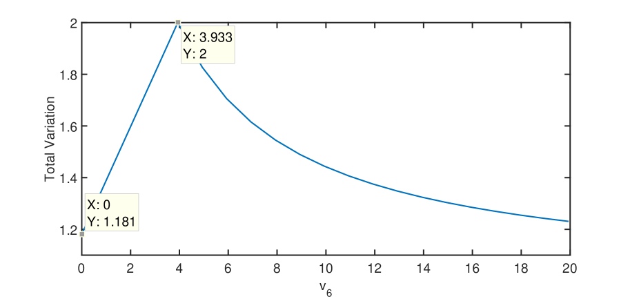
Figure 3: Total variation of the spectral component of $J_{2}(0)$ for the example in Section VI with respect to generalized eigenvector component $v_{6}$. The data points (gray squares) show total variation $1.181$ when $v_{6}=0$ and $2$ when $v_{6}=\frac{59}{15}$.

Total variation. Possible Jordan chains for the Jordan block $J_{2}(0)$ and their respective total variations (57) are computed. By applying the recurrence equation (5) with $\lambda=0$, the following eigenvector submatrices with columns that span potential Jordan subspaces corresponding to $J_{2}(0)$ in (92) are obtained:

$$V_{1} =\begin{bmatrix}-2&0&0&3&0&-2&5&0&0&0\\ 0&0&0&1&\frac{1}{2}&0&0&0&1&\frac{5}{3}\end{bmatrix}^{T},$$ (93)

$$V_{2} =\begin{bmatrix}-2&0&0&3&0&-2&5&0&0&0\\ 0&0&0&-\frac{1}{2}&\frac{1}{2}&1&0&0&1&\frac{5}{3}\end{bmatrix}^{T},$$ (94)

$$V_{3} =\begin{bmatrix}-2&0&0&3&0&-2&5&0&0&0\\ 0&0&0&-\frac{49}{10}&\frac{1}{2}&\frac{59}{15}&0&0&1&\frac{5}{3}\end{bmatrix}^{T}.$$ (95)

Normalizing these matrices by their L1 norm as specified by Property 22 in Section V, the resulting total variations (57) are

$$\mathrm{TV}_{G}(V_{1}) =1.181$$ (96)

$$\mathrm{TV}_{G}(V_{2}) =1.389$$ (97)

$$\mathrm{TV}_{G}(V_{3}) =2.$$ (98)

These results show that the degrees of freedom in the Jordan chain recurrence (5) can lead to fluctuating total variations of the spectral components.

We compare these results to the upper bound (67), which is $\left|\lambda-1\right|+1=2$ for $\lambda=0$. Our results show that this upper bound is achieved with $V_{3}$ (95). In this way, the class total variation (68) of the Jordan subspace $\mathscr{J}_{2}(0)=\mathrm{span}\{V_{3}\}$ corresponding to Jordan block $J_{2}(0)$ is

$$\mathrm{TV}_{\mathbf{G}_{A}^{J}}\left(\mathscr{J}_{2}(0)\right)=2.$$ (99)

This example shows that using the class total variation or the upper bound (67) as a method of ranking the spectral components by (57) removes the dependency on the choice of generalized eigenvector.

We modify $V_{3}$ (95) by varying the sixth component $v_{6}$ (and fourth component $v_{4}$ as $v_{4}=1-1.5v_{6}$) of the generalized eigenvector in the second column. It can be verified by (5) that such vectors are valid generalized eigenvectors. The results are shown in Figure 3 with the total variation plotted versus the value of $v_{6}$. The data point at $v_{6}=0$ corresponds to the total variation of $V_{1}$ (93). The figure illustrates that the total variation has a global maximum at $v_{6}=\frac{59}{15}$.

Jordan equivalence. It can be shown that the images of the projection matrices (12) corresponding to $V_{1}$(93), $V_{2}$ (94), and $V_{3}$ (95) are nonidentical; that is, each choice of Jordan basis corresponds to a different Jordan equivalence class.

Consider an alternate basis for $\mathscr{J}_{2}(0)=\mathrm{span}\{V_{3}\}$ provided by the columns of matrix

$$\widetilde{V}_{1}=\begin{bmatrix}1&0&0&3&0&1&2&0&0&0\\ 0&0&0&-1&\frac{1}{2}&1&0&0&1&\frac{5}{3}\end{bmatrix}^{T}.$$ (100)

If $\widetilde{V}$ is defined as the matrix consisting of the columns of $V$ that do not correspond to $\mathscr{J}_{2}(0)$ in addition to the columns of $\widetilde{V}_{1}$ (100), it can be shown that $\widetilde{A}=\widetilde{V}J\widetilde{V}^{-1}$ does not equal $A$. Nevertheless, the oblique projection matrices (12) corresponding to $\widetilde{V}_{1}$ (100) and $V_{3}$ (95) onto the Jordan subspaces are identical; that is, the GFT (1) is equivalent for both eigenvector matrices, and graphs $\mathcal{G}(A)$ and $\mathcal{G}(\widetilde{A})$ are in the same Jordan equivalence class corresponding to $\mathscr{J}_{2}(0)=\mathrm{span}\{V_{3}\}$. The total variation of $\widetilde{V}_{1}$ with respect to $\widetilde{A}$ is

$$\mathrm{TV}_{G}(\widetilde{V}_{1})=\left\|\widetilde{V}_{1}-\widetilde{A}\widetilde{V}_{1}\right\|_{1}=1.452.$$ (101)

Thus, $\widetilde{V}_{1}$ does not achieve the class total variation (99).

VII Limitations

The Jordan equivalence classes discussed in Section IV show that there are degrees of freedom over graph topologies with defective adjacency matrices that enable the GFT to be equivalent over multiple graph structures. It may be sufficient to find these classes by traversing the graph once (with total time complexity $O(\left|V\right|+\left|E\right|)$) and then determining the Jordan normal form of the underlying graph because of the acyclic and cyclic structures within the graph; see [24, 25] and more details in Section IV.

On the other hand, not all graphs have structures that readily reveal their Jordan equivalence classes. For example, arbitrary directed, sparse matrices such as road networks or social networks may have complex substructures that require a full eigendecomposition before determining the corresponding Jordan equivalence class. Inexact eigendecomposition methods are useful to approximate the GFT in this case. In particular, the authors explore such a method in [21].

VIII Conclusion

This paper characterizes two equivalence classes of graph structures that arise from the spectral projector-based GFT formulation of [12]. Firstly, isomorphic equivalence classes ensure that the GFT is equivalent with respect to a given node ordering. This allows the exploitation of banded matrix structures that permit efficient eigendecomposition methods. Secondly, Jordan equivalence classes show that the GFT can be identical over graphs of different topologies. Certain types of graphs have Jordan equivalence classes that can be determined by a single traversal over the graph structure, which means that the eigenvector matrix can potentially be chosen for a simpler matrix topology. For more general graphs for which the equivalence class cannot be easily determined, inexact methods such as those proposed in [21] provide a means to computing the spectral projector-based GFT.

Lastly, a total variation-based ordering of the Jordan subspaces is proposed. Since the total variation is dependent on the particular choice of Jordan basis, we propose a class variation-based ordering that is defined by the Jordan equivalence class of the graph.

References

- [1] A. Sandryhaila and J.M.F. Moura, “Discrete signal processing on graphs,” IEEE Transactions on Signal Processing, vol. 61, no. 7, pp. 1644–1656, Apr. 2013.
- [2] D. Shuman, S.K. Narang, P. Frossard, A. Ortega, and P. Vandergheynst, “The emerging field of signal processing on graphs: Extending high-dimensional data analysis to networks and other irregular domains,” IEEE Signal Processing Magazine, vol. 30, no. 3, pp. 83–98, Apr. 2013.
- [3] A. Sandryhaila and J.M.F. Moura, “Big data analysis with signal processing on graphs: Representation and processing of massive data sets with irregular structure,” IEEE Signal Processing Magazine, vol. 31, no. 5, pp. 80–90, Aug. 2014.
- [4] A. Sandryhaila and J.M.F. Moura, “Discrete signal processing on graphs: Frequency analysis,” IEEE Transactions on Signal Processing, vol. 62, no. 12, pp. 3042–3054, Jun. 2014.
- [5] O. Teke and P.P. Vaidyanathan, “Extending classical multirate signal processing theory to graphs – Part I: Fundamentals,” IEEE Transactions on Signal Processing, vol. 65, no. 2, pp. 409–422, Jan. 2017.
- [6] X. Zhu and M. Rabbat, “Approximating signals supported on graphs,” in Proceedings of the 37th IEEE International Conference on Acoustics, Speech, and Signal Processing (ICASSP), Mar. 2012, pp. 3921–3924.
- [7] S.K. Narang and A. Ortega, “Perfect reconstruction two-channel wavelet filter banks for graph structured data,” IEEE Transactions on Signal Processing, vol. 60, no. 6, pp. 2786–2799, Jun. 2012.
- [8] O. Teke and P.P. Vaidyanathan, “Extending classical multirate signal processing theory to graphs – Part II: M-channel filter banks,” IEEE Transactions on Signal Processing, vol. 65, no. 2, pp. 423–437, Jan. 2017.
- [9] A.G. Marques, S. Segarra, G. Leus, and A. Ribeiro, “Sampling of graph signals with successive local aggregations,” IEEE Transactions on Signal Processing, vol. 64, no. 7, pp. 1832–1843, Apr. 2016.
- [10] S. Segarra, A. Marques, G. Leus, and A. Ribeiro, “Reconstruction of graph signals through percolation from seeding nodes,” IEEE Transactions on Signal Processing, vol. 64, no. 16, pp. 4363–4378, Aug. 2016.
- [11] S. Chen, A. Sandryhaila, J.M.F. Moura, and J. Kovačević, “Signal recovery on graphs: Variation minimization,” IEEE Transactions on Signal Processing, vol. 63, no. 17, pp. 4609–4624, 2015.
- [12] J.A. Deri and J.M.F. Moura, “Spectral projector-based graph Fourier transforms,” submitted, Nov. 2016.
- [13] P. Lancaster and M. Tismenetsky, The Theory of Matrices, New York, NY, USA: Academic, 2nd edition, 1985.
- [14] R.A. Horn and C.R. Johnson, Matrix Analysis, Cambridge, U.K.: Cambridge Univ. Press, 2012.
- [15] I. Gohberg, P. Lancaster, and L. Rodman, Invariant Subspaces of Matrices with Applications, vol. 51, Philadelphia, PA, USA: SIAM, 2006.
- [16] G.H. Golub and C.F. Van Loan, Matrix Computations, Baltimore, MD, USA: JHU Press, 4 edition, 2013.
- [17] M. Vetterli, J. Kovačević, and V.K. Goyal, Foundations of Signal Processing, Cambridge, U.K.: Cambridge Univ. Press, 2014.
- [18] D.M. Cvetković, M. Doob, I. Gutman, and A. Torgašev, Recent results in the theory of graph spectra, vol. 36 of Annals of Discrete Mathematics, North-Holland, 1988.
- [19] E. Cuthill and J. McKee, “Reducing the bandwidth of sparse symmetric matrices,” in Proceedings of the 1969 24th National Conference, New York, NY, USA, 1969, ACM ’69, pp. 157–172.
- [20] Hwansoo Han and Chau-Wen Tseng, “A comparison of locality transformations for irregular codes,” in International Workshop on Languages, Compilers, and Run-Time Systems for Scalable Computers. Springer, 2000, pp. 70–84.
- [21] J.A. Deri and J.M.F. Moura, “Agile inexact methods for spectral projector-based graph Fourier transforms,” submitted, Nov. 2016.
- [22] C. Candan, “On the eigenstructure of DFT matrices [DSP education],” IEEE Signal Processing Magazine, vol. 28, no. 2, pp. 105–108, 2011.
- [23] L.K. Jørgensen, “On normally regular digraphs,” Tech. Rep. R 94-2023, Univ. of Aalborg, Institute for Electronic Systems, Dept. of Mathematics and Computer Science, 1994.
- [24] D.A. Cardon and B. Tuckfield, “The Jordan canonical form for a class of zero–one matrices,” Linear Algebra and its Applications, vol. 435, no. 11, pp. 2942–2954, 2011.
- [25] H. Nina, R.L. Soto, and D.M. Cardoso, “The Jordan canonical form for a class of weighted directed graphs,” Linear Algebra and its Applications, vol. 438, no. 1, pp. 261–268, 2013.
- [26] M. Püschel and J.M.F. Moura, “Algebraic signal processing theory: Foundation and 1-D time,” IEEE Transactions on Signal Processing, vol. 56, no. 8, pp. 3572–3585, Aug. 2008.
- [27] M. Püschel and J.M.F. Moura, “Algebraic signal processing theory: 1-D space,” IEEE Transactions on Signal Processing, vol. 56, no. 8, pp. 3586–3599, Aug. 2008.