DyMo: Dynamic Monitoring
of Large Scale LTE-Multicast Systems

Abstract

LTE evolved  Multimedia  Broadcast/Multicast Service (eMBMS) is an attractive solution for video delivery to very large groups in crowded venues. However, deployment and management of eMBMS systems is challenging, due to the lack of real-time feedback from the User Equipment (UEs). Therefore, we present the Dynamic Monitoring (DyMo) system for low-overhead feedback collection. DyMo leverages eMBMS for broadcasting Stochastic Group Instructions to all UEs. These instructions indicate the reporting rates as a function of the observed Quality of Service (QoS). This simple feedback mechanism collects very limited QoS reports from the UEs. The reports are used for network optimization, thereby ensuring high QoS to the UEs. We present the design aspects of DyMo and evaluate its performance analytically and via extensive simulations. Specifically, we show that DyMo infers the optimal eMBMS settings with extremely low overhead, while meeting strict QoS requirements under different UE mobility patterns and presence of network component failures. For instance, DyMo can detect the eMBMS Signal-to-Noise Ratio (SNR) experienced by the $0.1\%$ percentile of the UEs with Root Mean Square Error (RMSE) of $0.05\%$ with only 5 to 10 reports per second regardless of the number of UEs.

I Introduction

Wireless video delivery is an important service. However, unicast video streaming over LTE to a large user population in crowded venues requires a dense deployment of Base Stations (BSs) [1, 2, 3]. Such deployments require high capital and operational expenditure and may suffer from extensive interference between adjacent BSs.

LTE-eMBMS (evolved Multimedia Broadcast/Multicast Service) [4, 5] provides an alternative method for content delivery in crowded venues which is based on broadcasting to a large population of User Equipment (UEs) (a.k.a. eMBMS receivers). As illustrated in Fig. 1, in order to improve the Signal-to-Noise Ratio (SNR) at the receivers, eMBMS utilizes soft signal combining techniques. Thus, a large scale Modulation and Coding Scheme (MCS) adaptation should be conducted simultaneously for all the BSs based on the Quality of Service (QoS) at the UEs.

Unfortunately, the eMBMS standard [4] only provides a mechanism for UE QoS reporting once the communication terminates, thereby making it unsuitable for real-time traffic. Recently, the Minimization of Drive Tests (MDT) protocol [6] was extended to provide eMBMS QoS reports periodically from all the UEs or when a UE joins/leaves a BS. However, in crowded venues with tens of thousands of UEs (e.g., [1]), even infrequent QoS reports by each UE may result in high signaling overhead and blocking of unicast traffic. Due to the limited ability to collect feedback, a deployment of an eMBMS system is very challenging. In particular, it is hindered by the following limitations:

• Extensive and time consuming radio frequency surveys: Such surveys are conducted before each new eMBMS deployment. Yet, they provide only limited information from a few monitoring nodes.

• Conservative resource allocation: The eMBMS MCS and Forward Error Correction (FEC) codes are set conservatively to increase the decoding probability.

• Oblivious to environmental changes: It is impossible to infer QoS degradation due to environmental changes, such as new obstacles or component failures.

Figure 1: The DyMo system architecture: It exchanges control information with the Multicast Coordination Entity (MCE) of BSs which use soft signal combining for eMBMS. The Instruction Control module uses broadcast to dynamically partition the UEs into groups, each sending QoS reports at a different rate. The reports are sent to the Feedback Collection module and allow the QoS Evaluation module to identify an SNR Threshold. It is used by the MCS Control module to specify the optimal MCS to the MCEs.

Clearly, there is a need to dynamically tune the eMBMS parameters according to the feedback from UEs. However, a key challenge for eMBMS parameter tuning for large scale groups is obtaining accurate QoS reports with low overhead. Schemes for efficient feedback collection in wireless multicast networks have recently received considerable attention, particulalty in the context of WiFi networks (e.g., [7, 8, 9, 10]). Yet, WiFi feedback schemes cannot be easily adapted to eMBMS since unlike WiFi, where a single Access Point transmits to a node, transmissions from multiple BSs are combined in eMBMS. Efforts for optimizing eMBMS performance focus on periodically collecting QoS reports from all UEs (e.g., [11]) but such approaches rely on extensive knowledge of the user population (for more details, see Section II-B).

In this paper, we present the Dynamic Monitoring (DyMo) system designed to support efficient LTE-eMBMS deployments in crowded and dynamic environments by providing accurate QoS reports with low overhead. DyMo identifies the maximal eMBMS SNR Threshold such that only a small number of UEs with SNR below the SNR Threshold may suffer from poor service. To identify the SNR Threshold accurately, DyMo leverages the broadcast capabilities of eMBMS for fast dissemination of instructions to a large UE population.

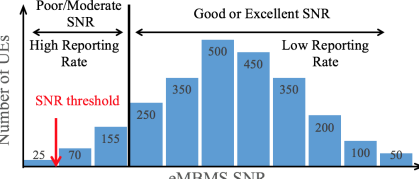
Each instruction is targeted at a sub-group of UEs that satisfies a given condition. It instructs the UEs in the group to send a QoS report with some probability during a reporting interval. We refer to these instructions as Stochastic Group Instructions. For instance, as shown in Fig. 2, DyMo divides UEs into two groups. UEs with poor or moderate eMBMS SNR are requested to send a report with a higher rate during the next reporting interval. In order to improve the accuracy of the SNR Threshold, the QoS reports are analyzed and the group partitions and instructions are dynamically adapted such that the UEs whose SNR is around the SNR Threshold report more frequently. The SNR Threshold is then used for setting the eMBMS parameters, such as the MCS and FEC codes.

From a statistics perspective, DyMo can be viewed as a practical method for realizing importance sampling [12] in wireless networks. Importance sampling improves the expectation approximation of a rare event by sampling from a distribution that overweighs the important region. With limited knowledge of the SNR distribution, DyMo leverages Stochastic Group Instructions to narrow down the SNR sampling to UEs that suffer from poor service and consequently obtains accurate estimation of the SNR Threshold. To the best of our knowledge, this is the first realization of using broadcast instructions for importance sampling in wireless networks.

Figure 2: Operation of DyMo for a sample UE QoS distribution: UEs are partitioned into two groups based on their SNR and each group is instructed to send QoS reports at a different rate. The partitioning is dynamically adjusted based on the reports to yield more reports from UEs whose SNR is around the estimated SNR Threshold.

The DyMo system architecture is illustrated in Fig. 1. It operates on an independent server and exchanges control information with several BSs supporting eMBMS. The Instruction Control module instructs the different groups to send reports at different rates. The reports are sent via unicast to the Feedback Collection module and allow the QoS Evaluation module to identify an accurate SNR Threshold. The SNR Threshold is determined such that only a predefined number of UEs with SNR below the threshold, termed as outliers, may suffer from poor service. The MCS Control module utilizes the SNR Threshold to configure the eMBMS parameters (e.g., MCS) accordingly. Finally, the QoS Evaluation module continually refines group partitions based on the reports.

We focus on the QoS Evaluation module and develop a Two-step estimation algorithm which can efficiently identify the SNR Threshold as a one time estimation. We also develop an Iterative estimation algorithm for estimating the SNR Threshold iteratively, when the distribution changes due to UE mobility or environmental changes, such as network component failures. Our analysis shows that the Two-step estimation and Iterative estimation algorithms can infer the SNR Threshold with a small error and limited number of QoS reports. It is also shown that they outperform the Order-Statistics estimation method, a well-known statistical method, which relies on sampling UEs with a fixed probability. For instance, the Two-step estimation requires only 400 reports when estimating the $1\%$ percentile to limit the error to $0.3\%$ for each re-estimation. The Iterative estimation algorithm performs even better than the Two-step estimation and the maximum estimation error can be bounded according to the maximum change of SNR Threshold.

We conduct extensive at-scale simulations, based on real eMBMS radio survey measurements from a stadium and an urban area. It is shown that DyMo accurately infers the SNR Threshold and optimizes the eMBMS parameters with low overhead under different mobility patterns and even in the event of component failures. DyMo significantly outperforms alternative schemes based on the Order-Statistics estimation method which rely on random or periodic sampling.

Our simulations show that both in a stadium-like and urban area, DyMo detects the eMBMS SNR value of the $0.1\%$ percentile with Root Mean Square Error (RMSE) of $0.05\%$ with only $5$ messages per second in total across the whole network. This is at least $8$ times better than Order-Statistics estimation based methods. DyMo also infers the optimal SNR Threshold with RMSE of $0.3$ dB regardless of the UE population size, while the error of the best Order-Statistics estimation method is above $1$ dB. DyMo violates the outlier bound (of $0.1\%$) with RMSE of at most $0.35$ while the best Order-Statistics estimation method incurs RMSE of over $4$ times. The simulations also show that after a failure, DyMo converges instantly (i.e., in a single reporting interval) to the optimal SNR Threshold. Thus, DyMo is able to infer the maximum MCS while preserving QoS constraints.

To summarize, the main contributions of this paper are three-fold:
(i) We present the concept of Stochastic Group Instructions for efficient realization of importance sampling in wireless networks.
(ii) We present the system architecture of DyMo and efficient algorithms for SNR Threshold estimation.
(iii) We show via extensive simulations that DyMo performs well in diverse scenarios.
The principal benefit of DyMo is its ability to infer the system performance based on a low number of QoS reports. It converges very fast to the optimal eMBMS configuration and it reacts very fast to changes in the environment. Hence, it eliminates the need for service planning and extensive field trials. Further, DyMo is compatible with existing LTE-eMBMS deployments and does not need any knowledge of the UE population.

The rest of the paper is organized as follows. We provide background information about eMBMS and a brief review of related work in Section II. We introduce the model and objective in Section III. We present the DyMo system in Section IV. The algorithms for SNR threshold estimation with their analysis are given in Section V. The numerical evaluation results appear in Section VI before concluding in Section VII. Some details of our analysis are given in the Appendix.

II Background information

II-A eMBMS Background

LTE-Advanced networks provide broadcast services by using evolved Multimedia Broadcast/Multicast Service (eMBMS) [13]. eMBMS is best suited to simultaneously deliver common content like video distribution to a large number of users within a contiguous region of cells. eMBMS video distribution is offered as an unidirectional service without feedback from the UE nor retransmissions of lost packets. This is enabled by all cells acting in a coordinated Single Frequency Network (SFN) arrangement, i.e., transmitting identical signals in a time synchronized manner, called Multicast Broadcast Single Frequency Network (MBSFN). The identical signals combine over the air in a non-coherent manner at each of the user locations, resulting in an improved Signal-Noise Ratio (SINR). Thus, what is normally out-of-cell interference in unicast becomes useful signal in eMBMS. For avoiding further interference from cells not transmitting the same MBSFN signal, the BSs near the boundary of the MBSFN area are used as a protection tier and they should not include eMBMS receivers in their coverage areas.

II-B Related Work

Wireless multicast control schemes received considerable attention in recent years (see survey in [7] and references therein). Below we briefly review the most relevant papers.

LTE-eMBMS: Most previous work on eMBMS (e.g., [14, 15, 16, 17]) assumes individual feedback from all the UEs and proposes various MCS selection or resource allocation techniques. Yet, extensive QoS reports impose significant overhead on LTE networks, which are already highly congested in crowded venues [1]. An efficient feedback scheme was proposed in [11] but it relies on knowledge of path loss (or block error) of the entire UE population to form the set of feedback nodes.

Recently, [18] proposed a multicast-based anonymous query scheme for inferring the maximum MCS that satisfies all UEs without sending individual queries. However, the scheme cannot be implemented in current LTE networks, since it will require UEs to transmit simultaneous beacon messages in response to broadcast queries.

WiFi Multicast: Most of the wireless multicast schemes are designed for WiFi networks. Some rely on individual feedback from all nodes for each packet [9, 10]. Leader-Based Schemes [19, 20, 21] collect feedback from a few selected nodes with the weakest channel quality. Cluster-Based Feedback Schemes in [8, 22] balance accurate reporting with minimization of control overhead by selecting nodes with the weakest channel condition in each cluster as feedback nodes.

However, WiFi multicast solutions cannot easily be applied to LTE-eMBMS systems. First, in WiFi, each node is associated with an Access Point, and therefore, the Access Point is aware of every node and can specify the feedback nodes. In LTE, eMBMS UEs could be in the idle state and the network may not be aware of the number of active UEs. Second, eMBMS is based on simultaneous transmission from various BSs. Thus, unlike in WiFi where MCS adaptation is done at each Access Point independently, a common MCS adaptation should be done at all BSs.

TABLE I: Notation.

Symbol	Semantics
$m$	The number of UEs in the venue, also the
	number of active eMBMS receiver in static settings.
$m(t)$	The number of active eMBMS receivers at time $t$.
$h_{v}(t)$	The individual SNR value of UE $v$
	at time interval $t$.
$s(t)$	The SNR Threshold at time $t$.
$p$	QoS Threshold - The maximal portion of UEs
	with individual SNR value $h_{v}(t)<s(t)$.
$r$	Overhead Threshold - An upper bound on the
	average number of reports in a reporting interval.

III Model and Objective

III-A Network Model

We consider an LTE-Advanced network with multiple base stations (BSs) providing eMBMS service to a very large group of $m$ UEs in a given large venue (e.g., sports arena, transportation hub). Such venues can accommodate tens of thousands of users. The eMBMS service is managed by a single DyMo server as shown in Fig. 1 and all the BSs transmit identical multicast signals in a time synchronized manner. The multicast flows contain FEC code that allows the UEs to tolerate some level of losses $\ell$ (e.g., up to $5\%$ packet losses).

All UEs can detect and report the eMBMS QoS they experience. More specifically, time is divided into short reporting intervals, a few seconds each. We assume that the eMBMS SNR distribution of the UEs does not change during each reporting interval. We define the individual SNR value $h_{v}(t)$, such that at least a given percentage $1-\ell$ (e.g., $95\%$) of the eMBMS packets received by an UE $v$ during a reporting interval $t$ have an SNR above $h_{v}(t)$. For a given SNR value, $h_{v}(t)$, there is a one-to-one mapping to an eMBMS MCS such that a UE can decode all the packets whose SNR is above $h_{v}(t)$ [16, 17]. The remaining packets $\ell$ can be recovered by appropriate level of FEC assuming $\ell$ is not too large. A summary of the main notations used throughout the paper are given in Table I.

III-B Objective

We aim to design a scalable efficient eMBMS monitoring and control system for which the objective is outlined below and that satisfies the following constraints:

• QoS Constraint – Given a QoS Threshold $p\ll 1$, at most a fraction $p$ of the UEs may suffer from packet loss of more than $\ell$. This implies that, with FEC, a fraction $1-p$ of the UEs should receive all of the transmitted data. We refer to the set UEs that suffer from packet loss after FEC as outliers and the rest are termed normal UEs.

• Overhead Constraint – The average number of UE reports during a reporting interval should be below a given Overhead Threshold $r$.

Objective: Accurately identify at any given time $t$ the maximum SNR Threshold, $s(t)$ that satisfies the QoS and Overhead Constraints.

Namely, the calculated $s(t)$ needs to ensure that a fraction $1-p$ of the UEs have individual SNR values $h_{v}(t)\geq s(t)$.

The network performance can be maximized by using $s(t)$ to calculate the maximum eMBMS MCS that meets the QoS constraint [16, 17]. This allows reducing the resource blocks allocated to eMBMS. Alternatively for a service such as video, the video quality can be enhanced without increasing the bandwidth allocated to the video flow.

IV The DyMo System

This section introduces the DyMo system. It first presents the DyMo system architecture, which is based on the Stochastic Group Instructions concept. Then, it provides an illustrative example of DyMo operations along with some technical aspects of eMBMS parameter tuning.

IV-A System Overview

We now present the DyMo system architecture, shown in Fig. 1.

Feedback Collection: This module operates in the DyMo server and in a DyMo Mobile-Application on each UE. At the beginning of each reporting interval, the Feedback Collection module broadcasts Stochastic Group Instructions to all the UEs. These instructions specify the QoS report probability as a function of the observed QoS (i.e., eMBMS SNR). In response, each UE independently determines whether it should send a QoS report at the current reporting interval.

QoS Evaluation: The UE feedback is used to estimate the eMBMS SNR distribution, as shown in Fig. 2. Since the system needs to determine the SNR Threshold, $s(t)$, the estimation of the low SNR range of the distribution has to be more accurate. To achieve this goal, the QoS Evaluation module partitions the UEs into two or more groups, according to their QoS values. This allows DyMo to accurately infer the optimal value of $s(t)$, by obtaining more reports from UEs with low SNR. We elaborate on the algorithms for $s(t)$ estimation in Section V.

MCS Control: Since the eMBMS signal is a combination of synchronized multicast transmissions from several BSs, the unicast SNR can be used as a lower bound on the eMBMS SNR. Therefore, the initial eMBMS MCS and FEC are determined from unicast SNR values reported by the UEs during unicast connections. Then, after each reporting interval, the QoS Evaluation module infers the SNR Threshold, $s(t)$, and the MCS Control module determines the desired eMBMS settings, mainly the eMBMS MCS and FEC, according to commonly used one-to-one mappings [16, 17].

TABLE II: Example of the DyMo feedback report overhead.

Group	No. of UEs	Report Prob.	Avg. reports per interval	Avg. per sec	Rate per min
H	$250$	$20\%$	$50$	$5$	$\approx 100\%$
L	$2250$	$2\%$	$45$	$\approx{5}$	$\approx{12}\%$

IV-B Illustrative Example

DyMo operations and the Stochastic Group Instructions concept are demonstrated in the following example. Consider an eMBMS system that serves $2,500$ UEs with the QoS Constraint that at most $p=1\%=25$ UEs may suffer from poor service. Assume a reporting interval of $10$ seconds. To infer the SNR Threshold, $s(t)$, that satisfies the constraint, the UEs are divided into two groups:

$\bullet~{}$ High-Reporting-Rate (H): $10\%~{}(250)$ of UEs that experience poor or moderate service quality report with probability of $20\%$, i.e., an expected number of $50$ reports per interval.

$\bullet~{}$ Low-Reporting-Rate (L): $90\%~{}(2250)$ of the UEs that experience good or excellent service quality report with probability of $2\%$, implying about $45$ reports per interval.

Table II presents the reporting probability of each UE and the number of QoS reports per reporting interval by each group. It also shows the number of QoS reports per second and the reporting rate per minute (i.e., the expected fraction of UEs that send QoS reports in a minute). Since the QoS Constraint implies that only 25 UEs may suffer from poor service, these UEs must belong to group H. Although only $10$ QoS reports are received at each second, all the UEs in group H send QoS reports at least once a minute. Thus, the SNR Threshold can be accurately detected within one minute.

IV-C Dynamic eMBMS Parameter Tuning

Besides the MCS, DyMo can leverage the UE feedback and the calculated SNR Threshold, $s(t)$, for optimizing other eMBMS parameters including FEC, video coding and protection tier. While this aspect is not the focus of this study, we briefly discuss the challenges and the solutions for dynamic tuning of the eMBMS parameters.

Once the SNR Threshold $s(t)$ is selected, DyMo tunes the eMBMS parameters accordingly. Every time DyMo changes the eMBMS parameters, the consumption of wireless resources for the service is affected as well. For instance, when the eMBMS MCS index is increased, some of the wireless resources allocated for eMBMS are not needed and can be released. Alternatively, the service provider may prefer to improve the video quality by instructing the content server to increase the video resolution. Similarly, before the eMBMS MCS index is lowered, the wireless resources should be increased or the video resolution should be reduced to match the content bandwidth requirements to the available wireless resources.

Since the eMBMS signal is a soft combination of the signals from all BSs in the venue, any change of eMBMS parameters must be synchronized at all the BSs to avoid interruption of service. The fact that all the clocks of the BSs are synchronized can be used and a scheme similar to the two phase commit protocol (which is commonly used in distributed databases [23]) can be used.

V Algorithms for SNR Threshold Estimation

This section describes the algorithms utilized by DyMo for estimating the SNR Threshold, $s(t)$, for a given QoS Constraint, $p$ and Overhead Constraint $r$. In particular, it addresses the challenges of partitioning the UEs into groups according to their SNR distribution as well as determining the group boundaries and the reporting rate from the UEs in each group, such that the overall estimation error of $s(t)$ is minimized. We first consider a static setting with fixed number of eMBMS receivers, $m$, where the SNR values of UEs are fixed. Then, we extend our solution to the case of dynamic environments and UE mobility.

V-A Order Statistics

We first briefly review a known statistical method in quantile estimation, referred to as Order-Statistics estimation. It provides a baseline for estimating $s(t)$ and is also used by DyMo for determining the initial SNR distribution in its first iteration assuming a single group. Let $F(x)$ be a Cumulative Distribution Function (CDF) for a random variable $X$, the quantile function $F^{-1}(p)$ is given by, $\inf\{x\mid F(x)\geq p\}$.

Let $X_{1},X_{2},\ldots,X_{r}$ be a sample from the distribution $F$, and $F_{r}$ its empirical distribution function. It is well known that the empirical quantile $F_{r}^{-1}(p)$ converges to the population quantile $F^{-1}(p)$ at all points $p$ where $F^{-1}$ is continuous [24]. Moreover, the true quantile, $\hat{p}=F(F_{r}^{-1}(p))$, of the empirical quantile estimate $F_{r}^{-1}(p)$ is asymptotically normal [24] with mean $p$ and variance

$$\operatorname*{\mathbb{V}ar}[\hat{p}]=\frac{p(1-p)}{r}$$ (1)

For SNR Threshold estimation, $F$ is the SNR distribution of all UEs. A direct way to estimate the SNR Threshold $s(t)$ is to collect QoS reports from $r$ randomly selected UEs, and calculate the empirical quantile $F_{r}^{-1}(p)$ as an estimate.

V-B The Two-Step Estimation Algorithm

We now present the Two-step estimation algorithm that uses two groups for estimating the SNR Threshold, $s(t)$, in a static setting. We assume a fixed number of UEs, $m$, and a bound $r$ on the number of expected reports. By leveraging Stochastic Group Instructions, DyMo is not restricted to collecting reports uniformly from all UEs and can use these instructions to improve the accuracy of $s(t)$. One way to realize this idea is to perform a two-step estimation that approximates the shape of the SNR distribution before focusing on the low quantile tail. The Two-step estimation algorithm works as follows:

Algorithm 1: Two-Step Estimation for the Static Case

1. Select $p_{1}$ and $p_{2}$ such that $p_{1}p_{2}=p$. Use $p_{1}$ as the percentile boundary for defining the two groups.

2. Select number of reports $r_{1}$ and $r_{2}$ for each step such that $r_{1}+r_{2}=r$.

3. Instruct all UEs to send QoS reports with probability $r_{1}/m$ and use these reports to estimate the $p_{1}$ quantile $\hat{x}_{1}=F_{r_{1}}^{-1}(p_{1})$.

4. Instruct UEs with SNR value below $\hat{x}_{1}$ to send reports with probability $r_{2}/(p_{1}\cdot m)$ and calculate the $p_{2}$ quantile $\hat{x}_{2}\!=\!G_{r_{2}}^{-1}(p_{2})$ as an estimation for $s(t)$ ($G$ is the CDF of the subpopulation with SNR below $\hat{x}_{1}$). ($G_{r_{2}}$ is the empirical CDF of the subpopulation with SNR below $\hat{x}_{1}$).

Upper Bound Analysis of the Two-Step Algorithm: To simplify the notation, we use $r_{1}$ and $r_{2}$ to denote the expected number of reports at each step. From (1) we know that

$$\hat{p}_{1}=F(\hat{x}_{1})~{}~{}~{}and~{}~{}~{}\hat{p}_{2}=G(\hat{x}_{2})$$

are unbiased estimators of $p_{1}$ and $p_{2}$ with variance

$$\operatorname*{\mathbb{V}ar}[\hat{p}_{1}]=\frac{p_{1}(1-p_{1})}{r_{1}}~{}~{}and~{}~{}\operatorname*{\mathbb{V}ar}[\hat{p}_{2}]=\frac{p_{2}(1-p_{2})}{r_{2}}$$ (2)

Our estimate $\hat{x}_{2}$ has true quantile $\hat{p}_{1}\hat{p}_{2}$. Assume $\hat{p}_{1}$ is less than $p_{1}+\epsilon_{1}$ and $\hat{p}_{2}$ is less than $p_{2}+\epsilon_{2}$ with high probability (for example, we can take $\epsilon_{1}$ and $\epsilon_{2}$ to be 3 times the standard deviation for $>99.8\%$ probability). Then, the over-estimation error is bounded by

$$\begin{split}\epsilon=\ &(p_{1}+\epsilon_{1})(p_{2}+\epsilon_{2})\ -\ p\\ =\ &p_{1}p_{2}+\epsilon_{1}p_{2}+\epsilon_{2}p_{1}+\epsilon_{1}\epsilon_{2}-p\\ \approx\ &\epsilon_{1}p_{2}+\epsilon_{2}p_{1}\end{split}$$ (3)

after ignoring the small higher order term $\epsilon_{1}\epsilon_{2}$. The case for under-estimation is similar. As shown in the Appendix, the error is minimized by taking,

$$p_{1}\!=\!p_{2}\!=\!\sqrt{p}~{}~{}~{}and~{}~{}~{}r_{1}\!=\!r_{2}\!=\!r/2$$

so that

$$\epsilon_{1}\!=\!\epsilon_{2}\!=\!3\sqrt{\sqrt{p}(1-\sqrt{p})/(r/2)}$$

This leads to proposition 1.

Proposition 1.

The distance between $p$ and the quantile of the Two-Step estimator $\hat{x}_{2}$, $\hat{p}=F^{-1}(x_{2})$, is bounded by

$$6\sqrt{2}\sqrt{\frac{p\sqrt{p}(1-\sqrt{p})}{r}}$$

with probability at least $1-2(1-\Phi(3))>99.6\%$, where $\Phi$ is the normal CDF.

We now compare this result against the bound of 3 standard deviations in the Order Statistics case, which is $3\sqrt{p(1-p)/r}$. With some simple calculations, it can be easily shown that if $p\leq 1/49\approx 2\%$, the Two-step estimation has smaller error than the Order-Statistics estimation method. Essentially the Order-Statistics estimation method has an error of order $\sqrt{p}/\sqrt{r}$, while the Two-step estimation has an error of order $p^{3/4}/\sqrt{r}$. Since $p\ll 1$, the difference can be significant.

Example: We validated the error estimation of the Two-step estimation algorithm and the Order-Statistics estimation method by numerical analysis. We considered the cases of $p=1\%$ and $p=0.1\%$ of uniform distribution on $[0,1]$ using $r\!=\!400$ samples over population size of $10^{6}$. The Two-step estimation algorithm has smaller standard error compared to the Order-Statistics estimation, as shown in Fig. 3. Its accuracy is significantly better for very small $p$.

The Two-step estimation algorithm can be generalized to 3 or more telescoping group sizes, but $p$ will need to be much smaller for these sampling schemes in order to reduce the number of samples.

V-C The Iterative Estimation Algorithm

We now turn to the dynamic case in which DyMo uses the SNR Threshold estimation $s(t-1)$ from the previous reporting interval to estimate $s(t)$ at the end of reporting interval $t$. Assume that the total number of eMBMS receivers, $m$, is fixed and it is known initially.

Suppose that DyMo has a current estimate $\hat{x}$ of the SNR threshold, $s(t)$, and $s(t)$ changes over time. We assume that the change in SNR of each UE is bounded over a time period. Formally,

$$|h_{v}(t_{1})-h_{v}(t_{2})|\leq L|t_{1}-t_{2}|$$

where $L$ is a Lipschitz constant for SNR changes. For example, we can assume that the UEs’ SNR cannot change by more than $5$dB during a reporting interval. This implies that within the interval, only UEs with SNR below $\hat{x}+5$dB affect the estimation of the $p$ quantile (subject to small estimation error in $\hat{x}$).

DyMo only needs to monitor UEs with SNR below $x_{L}=\hat{x}+L$. Denote the true quantile of $x_{L}$, defined by $F^{-1}(x_{L})$, as $p_{L}$. To apply a process similar to the second step of the Two-step estimation algorithm by focusing on UEs with SNR below $x_{L}$, first an estimate of $p_{L}$ is required. DyMo uses the previous SNR distribution to estimate $p_{L}$ and instructs the UEs to send reports at a rate $q=r/(p_{L}\cdot m)$. Let $Y$ be the number of reports received during the last reporting interval, then $Y/m\cdot q$ can be used as an updated estimator, $\hat{p_{L}}$, for $p_{L}$. This estimator is unbiased and has variance

$$\operatorname*{\mathbb{V}ar}[\hat{p_{L}}]=\operatorname*{\mathbb{V}ar}[\frac{Y}{m\cdot q}]=\frac{p_{L}}{m}\frac{1-q}{q}$$ (4)

As a result, the Iterative Estimation algorithm works as follows:

Algorithm 2: Iterative Estimation for the Dynamic Case

1. Instruct UEs with SNR below $\hat{x}+L$ to send reports at a rate $q$. Construct an estimator $\hat{p}_{L}$ of $p_{L}$ from the number of received reports $Y$.

2. Set $p^{\prime}=p/\hat{p}_{L}$. Find the $p^{\prime}$ quantile $x^{\prime}=G_{Y}^{-1}(p^{\prime})$ and report it as the $p$ quantile of the whole population ($G$ is the CDF of the subpopulation with SNR below $\hat{x}+L$).

Figure 3: Estimates of (a) $p=1\%$ and (b) $p=0.1\%$ quantiles for 500 runs for the Order-Statistics estimation (1-step) method and the Two-step estimation algorithm.

Upper Bound Analysis of the Iterative Algorithm: Suppose the estimation error of $p_{L}$ is bounded by $\epsilon_{1}$, and the estimation error of $p^{\prime}=p/\hat{p}_{L}$ is bounded by $\epsilon_{2}$ with high probability. Then, the estimation error is

$$\epsilon=(\frac{p}{\hat{p}_{L}}\pm\epsilon_{2})p_{L}-p=(\frac{p}{p_{L}\pm\epsilon_{1}}\pm\epsilon_{2})p_{L}-p.$$

The over-estimation error is bounded by

$$\frac{p}{p_{L}-\epsilon_{1}}\epsilon_{1}+p_{L}\epsilon_{2}.$$ (5)

If we assume $p_{L}-\epsilon_{1}\geq p$ (we know $p_{L}\geq p$ by the Lipschitz assumption), then the bound can be simplified to $\epsilon_{1}+p_{L}\epsilon_{2}$. The same bound also works for the under-estimation error. If $r$ denotes also the expected number of samples collected, $r=p_{L}\cdot m\cdot q$. The standard deviation of $\hat{p}_{L}$ can be written as:

$$\sqrt{\frac{p_{L}}{m}\frac{1-q}{q}}=\sqrt{\frac{p_{L}^{2}}{r}(1-\frac{r}{p_{L}m})}\leq\frac{p_{L}}{\sqrt{r}}.$$

If we assume $\epsilon_{1}=3p_{L}/\!\sqrt{r}$, the error of $\hat{p}_{L}$ is less than $\epsilon_{1}$ with probability at least $\Phi(3)$. Since we assume $p_{L}\!-\!\epsilon_{1}\!\geq\!p$ above, this implies $(1\!-\!3/\sqrt{r})p_{L}\!\geq\!p$. If $r\!\geq\!100$, then $p\!<\!0.7p_{L}$ will satisfy our requirement.

The standard deviation of estimating the $p^{\prime}=p/\hat{p}_{L}$ quantile is

$$\sqrt{\frac{1}{Y}\frac{p}{\hat{p}_{L}}(1-\frac{p}{\hat{p}_{L}})}\leq\frac{1}{2\sqrt{Y}},$$ (6)

by using the fact that $x(1-x)\leq 1/4$ for $x\in[0,1]$ and $Y$ is the number of reports received (a random variable). If the expected number of reports ${r}$ is reasonably large ($\geq 100$, say), then $Y$ can be well approximated by a normal and $Y\geq 0.7{r}$ with high probability $\Phi(3)=99.8\%$. Then, (6) is bounded by $2/(3\sqrt{{r}})\geq 1/(2\sqrt{0.7r})$ with high probability ($\Phi(3)=99.8\%$), and we can set $\epsilon_{2}=2/\sqrt{{r}}$. Substituting these back into (5), gives us the following proposition.

Proposition 2.

The distance between $p$ and the quantile of the estimator $x$, $\hat{p}=F^{-1}(x)$, is approximately bounded by

$$5\frac{p_{L}}{\sqrt{r}}$$

with probability at least $1-2(1-\Phi(3))>99.6\%$, if the expected sample size ${r}\geq 100$ and $p\leq 0.7p_{L}$.

This shows that the error is of order $p_{L}/\sqrt{{r}}$. We can see that the estimation error can be smaller compared to the error of order $p^{3/4}/\sqrt{{r}}$ in the static Two-step estimation if $p_{L}$ is small (i.e., the SNR of individual users does not change much during a reporting interval).

Exponential Smoothing: DyMo applies exponential smoothing by weighing past and current reports to smooth the estimates of the SNR Threshold, $s(t)$, and take older reports into account. It estimates the SNR Threshold as

$$s(t)=\alpha\hat{x}(t)+(1-\alpha)s(t-1)$$

where $\hat{x}(t)$ is the new raw SNR Threshold estimate using the Iterative estimation above and $s(t-1)$ is the SNR Threshold from the previous reporting interval. We set $\alpha=0.5$ to allow some re-use of past reports without letting them have too strong an effect on the estimates (e.g., samples older than 7 reporting intervals have less than 1% weight). DyMo also uses the exponential smoothing method for estimating the SNR distribution while taking into account QoS reports from previous reporting intervals.

Dynamic and Unknown Number of eMBMS Receivers: If the total number of UEs, $m(t)$, is unknown or changes dynamically, DyMo can estimate $m(t)$ by requiring UEs above the threshold $\hat{x}+L$ to send reports. These UEs can send reports at a lower rate, since $m(t)$ is not expected to change rapidly. Similar to the Two-step estimation algorithm, DyMo allocates $r_{1}=r_{2}=r/2$ reports to each group. The errors in estimating the total number of UEs $m(t)$ will contribute to the error $\epsilon_{1}$ in the estimation of $p_{L}$ in (5). The error analysis in this case is largely similar.

VI Performance Evaluation

Figure 4: (a) The heatmap of SNR distribution of UEs (b) the evolution of the number of active UEs over time compared to the number estimated by DyMo for a homogeneous environment.

Figure 5: (a) The heatmap of UE SNR distribution in a stadium area of $1000\times 1000m^{2}$ and (b) the evolution of the number of active UEs over time compared to the number estimated by DyMo for a stadium environment.

Figure 6: The heatmap of the SNR distribution of UEs (a) before a failure and (b) after a failure.

VI-A Methodology

We perform extensive simulations to evaluate the performance of DyMo with various values of QoS Constraint, $p$, Overhead Constraint, $r$, and number of UEs, $m$. Our evaluation considers dynamic environments with UE mobility and a changing number of active eMBMS receiversdenoted by $m(t)$, dynamically selected from the given set of $m$ UEs in the considered venue. In this paper, we present a few sets of simulation results, which capture various levels of variability of the SNR threshold, $s(t)$, over time.

We consider a variant of DyMo where the number of active UEs is unknown and is estimated from its measurements. We compare the performance of DyMo to four other schemes. To demonstrate the advantages of DyMo, we augment each scheme with additional information, which is hard to obtain in practice. The evaluated benchmarks are the following:

$~{}\bullet$ Optimal – Full knowledge of SNR values of the UEs at any time and consequently accurate information of the SNR distribution. This is the best possible benchmark although impractical, due to its high overhead.

$~{}\bullet$ Uniform – Full knowledge of the SNR characteristics at any location while assuming uniform UE distribution and static eMBMS settings. In practice, this knowledge cannot be obtained even with rigorous field trial measurements.

$~{}\bullet$ Order-Statistics – It is based estimation of the SNR Threshold using random sampling. The active UEs send reports with a fixed probability of $r/\operatorname*{\mathbb{E}}[m(t)]$ per second, assuming that the expected number of active UEs, $\operatorname*{\mathbb{E}}[m(t)]$, is known. We assume that the UEs are configured with this reporting rate during initialization. In practice, $\operatorname*{\mathbb{E}}[m(t)]$ is not available. We also ignore initial configuration overhead in our evaluation. Order-Statistics is the best possible approach when not using broadcast messages for UE configuration. We consider two variants of Order-Statistics. The first is Order-Statistics w.o. History which ignores SNR measurements from earlier reporting intervals. The second variant Order-Statistics w. History considers the history of reports.

Both DyMo and Order-Statistics w. History perform the same exponential smoothing process for assigning weights to the measurements from previous reporting intervals with a smoothing factor of $\alpha=0.5$. We use the following metrics to evaluate the performance of the schemes:

• Accuracy – The accuracy of the SNR Threshold estimation, $s(t)$. After calculating $s(t)$ at each reporting interval, we check the actual SNR Threshold Percentile in the accurate SNR distribution of the considered scheme. This metric provides the percentile of active UEs with individual SNR values below $s(t)$.

• QoS Constraint violation – The number of outliers above the QoS Constraint $p$. The number of outliers of a scheme in a given reporting interval $t$ is defined as the actual SNR Threshold Percentile of the scheme times the number of active eMBMS receivers, $m(t)$, at time $t$.

• Overhead Constraint violation – The number of reports above the Overhead Threshold, $r$, at each reporting interval.

The total simulation time for each instance is $30$mins with $5$ reporting intervals per minute (each is $12$s). During each reporting interval, an active UE may send its SNR value at most once. The accuracy of each SNR report is $0.1$dB.

VI-B Simulated Environments

We simulated a variety of environments with different SNR distributions and UE mobility patterns. Although the simulated environments are artificial, their SNR distributions mimic those of real eMBMS networks obtained through field trial measurements. To capture the SNR characteristics of an environment, we divide its geographical area into rectangles of $10m\times 10m$. For each reporting interval, each UE draws its individual SNR value, $h_{v}(t)$, from a Gaussian-like distribution which is a characteristic of the rectangle in which its located. The rectangles have different mean SNR, but the same standard deviation of roughly $5$dB (as observed in real measurements). Thus, the SNR characteristics of each environment are determined by the mean SNR values of the rectangles at any reporting interval. To demonstrate the performance of the different schemes, we discuss three types of environments.

$~{}\bullet$ Homogeneous: In the homogeneous setting the mean SNR value of each rectangle is fixed and it is uniformly selected in the range of $5-25$dB. Fig. 4 provides an example of the mean SNR values of such a venue as well as typical UE location distribution. In such instances, we assume random mobility pattern, in which each UE moves back and forth between two uniformly selected points. During the simulation, $50\%$ of the UEs are always active, while the other $50\%$ join and leave at some random time, as illustrated by Fig. 4. As we show later in such setting $s(t)$ barely change over time.

$~{}\bullet$ Stadiums: In a stadium, the eMBMS service quality is typically significantly better inside the stadium than in the surrounding vicinity (e.g., the parking lots). To capture this, we simulate several stadium-like environments, in which the stadium, in the center of the venue, has high eMBMS SNR with mean values in the range of $15-25$dB. On the other hand, the vicinity has significantly lower SNR with means values of $5-10$dB. An example of a stadium is shown in Fig. 5.

We assume a mobility pattern in which, the UEs move from the edges to the inside of the stadium in $12$mins, stay there for $3$mins, and then go back to the edges. As shown in Fig. 5, as the UEs move toward the center, the number of active UEs gradually increases from $10\%$ of the UEs to $100\%$, and then declines again as they move away.

$~{}\bullet$ Failures: Such an environment is similar to the homogeneous setting with a sudden event of a component failure. In the case of a malfunctioning component, the QoS in some parts of a venue can degrade significantly. To simulate failures, we consider cases in which the eMBMS SNR is high with a mean between $15-25$dB. During the simulation, (around the $10^{th}$ minute), we mimic a failure by reducing the mean SNR values of some of the rectangles by over $10$dB to the range of $5-10$dB. The mean SNR values are restored to their original values after a few minutes. Figs. 6 and 6 provide an example of the mean SNR values of such a venue before and after a failure, respectively. We assume the same mobility pattern like the homogeneous setting, as shown by Fig. 4.

Figure 7: Simulation results from a single simulation instance lasting for $30$mins in a component homogeneous environment with $20,000$ UEs moving side to side between two random points, with $p=0.1$ and $r=5$ messages/sec. (a) The actual percentile of the SNR Threshold estimated by DyMo, (b) the actual percentile of the SNR Threshold estimated by Order-Statistics, (c) the SNR Threshold estimation, (d) spectral Efficiency of Optimal vs. DyMo, (e) spectral Efficiency of Optimal vs. Order-Statistics, (f) the number of Outliers by using DyMo, (g) the number of outliers by using Uniform and Order-Statistics, and (h) the QoS report overhead.

Figure 8: Simulation results from a single simulation instance lasting for $30$mins in a stadium environment with $20,000$ UEs moving from the edges to the center and back, with $p=0.1$ and $r=5$ messages/sec. (a) The actual percentile of the SNR Threshold estimated by DyMo, (b) the actual percentile of the SNR Threshold estimated by Order-Statistics, (c) the SNR Threshold estimation, (d) spectral efficiency of Optimal vs. DyMo, (e) spectral efficiency of Optimal vs. Order-Statistics, (f) the number of Outliers by using DyMo, (g) the number of Outliers by using Uniform and Order-Statistics, and (h) the QoS report overhead.

Figure 9: Simulation results from a single simulation instance lasting for $30$mins in a component failure environment with $20,000$ UEs moving side to side between two random points, with $p=0.1$ and $r=5$ messages/sec. (a) The actual percentile of the SNR Threshold estimated by DyMo, (b) the actual percentile of the SNR Threshold estimated by Order-Statistics, (c) the SNR Threshold estimation, (d) spectral Efficiency of Optimal vs. DyMo, (e) spectral Efficiency of Optimal vs. Order-Statistics, (f) the number of Outliers by using DyMo, (g) the number of outliers by using Uniform and Order-Statistics, and (h) the QoS report overhead.

Figure 10: The Root Mean Square Error (RMSE) of different parameters averaged over 5 different simulation instances lasting for $30$mins each in homogeneous scenario with different SNR characteristics and UE mobility patterns. (a) SNR Threshold percentile RMSE vs. the total number of UEs in the system, (b) SNR Threshold percentile RMSE vs. the QoS Constraint $p$, (c) SNR Threshold percentile RMSE vs. the number of permitted reports , (d) Overhead RMSE vs. the number of UEs, (e) Overhead RMSE vs. the QoS constraint $p$, and (f) Overhead RMSE vs. the number of permitted reports.

Figure 11: The Root Mean Square Error (RMSE) of different parameters averaged over 5 different simulation instances lasting for $30$mins each in a stadium environment with different SNR characteristics and UE mobility patterns. (a) SNR Threshold percentile RMSE vs. the total number of UEs in the system, (b) SNR Threshold percentile RMSE vs. the QoS Constraint $p$, (c) SNR Threshold percentile RMSE vs. the number of permitted reports, (d) Overhead RMSE vs. the number of UEs, (e) Overhead RMSE vs. the QoS constraint $p$, and (f) Overhead RMSE vs. the number of permitted reports.

Figure 12: The Root Mean Square Error (RMSE) of different parameters averaged over 5 different simulation instances lasting for $30$mins each in failure scenario with different SNR characteristics and UE mobility patterns. (a) SNR Threshold percentile RMSE vs. the total number of UEs in the system, (b) SNR Threshold percentile RMSE vs. the QoS Constraint $p$, (c) SNR Threshold percentile RMSE vs. the number of permitted reports , (d) Overhead RMSE vs. the number of UEs, (e) Overhead RMSE vs. the QoS constraint $p$, and (f) Overhead RMSE vs. the number of permitted reports.

VI-C Performance over time

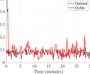
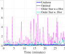
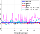
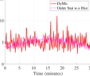
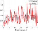
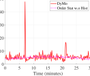
We first illustrate the performance of the different schemes over time for three given instances, a homogeneous, a stadium and a failure scenarios, with $m=20,000$ UEs, QoS Constraint $p=0.1\%$, and Overhead constraint $r=5$ reports/sec, i.e., $60$ messages per reporting interval. The number of permitted outliers depends on the number of active UEs at the current reporting interval. In the three considered scenarios, it can be at most $20$ at any given time. The key difference between the different instances is the rate at which the SNR Threshold changes. In the homogeneous environment the SNR Threshold is almost fixed with very limited variability. In the case of the stadium, the SNR Threshold gradually changes as the UEs change their locations. In the failure scenario, the SNR Threshold is roughly fixed but it drops instantly by $10$dBs for the duration of the failure.

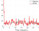
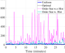
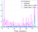
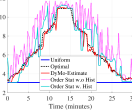
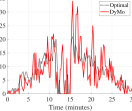
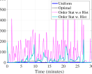
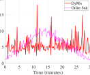
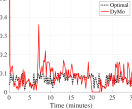
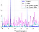
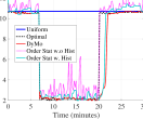
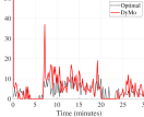
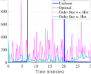
The results of the homogeneous, stadium and failure cases are shown in Figs. 7,  8 and 9, respectively. Figs. 7, 7,  8, 8, 9, and 9 show the actual SNR Threshold percentile over time. From Figs. 7, 8 and 9, we observe that DyMo can accurately infer the SNR Threshold with an estimation error of at most $0.1\%$. Fig. 9 shows slightly higher error of $0.25\%$ at the time of the failure (at the $7^{th}$ minute). The Order-Statistics variants suffer from much higher estimation error to the order of a few percentage points, as shown by Figs. 8, 8 and 8. This performance gap results in different estimation accuracy of the SNR Threshold for DyMo and Order-Statistics schemes as illustrated in Figs. 7, 8 and 9, respectively. These figures show that the performance of DyMo and Optimal is almost identical. Even in the event of a failure, DyMo reacts immediately and detects the SNR Threshold accurately. The Order-Statistics variants react quickly to a failure but not as accurately as DyMo. After the recovery, both DyMo and Order-Statistics w. History gradually increase their SNR Threshold estimates, due to the exponential smoothing process.

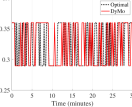
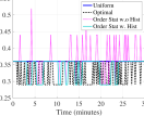
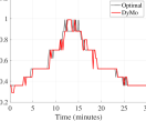
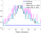
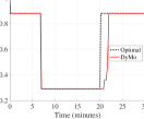
The SNR Threshold estimation gap directly impacts the number of outliers as well as the network utilization, i.e., the spectral efficiency. Figs. 7 and 7 show the number of outliers of DyMo and Order-Statistics variants for the homogeneous environment, respectively, while Figs. 7 and 7 show the spectral efficiency of the schemes. Figs. 7 and 7 reveal that after a short adaptation phase DyMo converges to the optimal performance, i.e., spectral efficiency, while preserving the QoS constraint. Fig. 7 show that both Optimal and DyMo fluctuate between two spectral efficiency levels, $0.29$ and $0.36$ bit/sec/Hz, which results from oscillatation between two MCS levels $3$ and $4$. Such oscillations can be easily suppressed by enforcing some delay between MCS increase operations. The Order-Statistics variants over estimate the SNR threshold and suffer from higher number of outliers, as shown by Fig. 7. The homogeneous setting represents quasi-static environments with minor variation of the SNR threshold, $s(t)$. In such settings, the Uniform scheme provides a good estimation of $s(t)$ and its number of outliers as well as the obtained spectral efficiency are comparable to DyMo. However, this is not the situation when $s(t)$ is time varying.

The number of outliers of DyMo and Order-Statistics variants for the stadium environment is shown in Figs. 8 and 8, respectively, while Figs. 9 and 9 illustrate the number of outliers of DyMo and Order-Statistics variants for the failure scenario, in this order. These figures show that the number of outliers that results from the Order-Statistics w. History and Order-Statistics w.o. History variants are occasionally over $200$ and $800$, respectively. Whereas, DyMo ensures that the number of outliers at any time is comparable to Optimal and in the worst case it exceeds the permitted number by less than a factor of $2$.

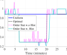
Figs. 8 and 8 show the spectral efficiency for the stadium environment, whereas Figs. 9 and 9 show the spectral efficiency for the component failure case. The spectral efficiency for each case is correlated to the SNR Threshold. For the stadium environment, DyMo has spectral efficiency close to Optimal while Uniform has the lowest spectral efficiency. In the event of a failure, the spectral efficiency of DyMo follows the Optimal as expected from the SNR Threshold estimations. Since Order-Statistics variants typically over estimate the SNR Threshold, they frequently determine MCS and consequently spectral efficiency that exceed the optimal settings. Such inaccuracy leads to a high number of outliers.

Figs. 7, 8  and 9 indicate only mild violation of the Overhead Constraint by both the DyMo and Order-Statistics variants. We observe that accurate SNR Threshold estimation allows DyMo to achieve near optimal spectral efficiency with negligible violation of the QoS Constraint. The other schemes suffer from sub-optimal spectral efficiency, excessive number of outliers, or both. Given that the permitted number of outliers is at most $20$, the Order-Statistics w. History and Order-Statistics w.o. History schemes exceed this value sometimes by a factor of $10$ and $40$, respectively. Among these two alternatives, Order-Statistics w. History leads to lower number of outliers. While Uniform provides accurate estimation of $s(t)$ for the homogeneous environment, we observe that it yields a very conservative eMBMS MCS setting in the stadium example, which causes low network utilization. In the failure scenario, the conservative eMBMS MCS of Uniform is not sufficient to cope with the low SNR Threshold and it leads to excessive number of outliers.

VI-D Impact of Various Parameters

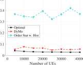
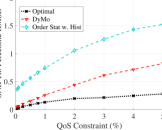
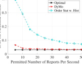
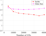
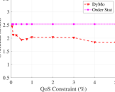
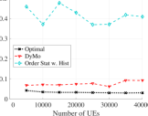
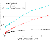
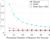
We now turn to evaluate the quality of the SNR Threshold estimation and the schemes’ ability to preserve the QoS and Overhead Constraints under various settings. We use the same configuration of $m=20,000$ UEs, $p=0.1\%$ and $r=5$ reports/sec and we evaluate the impact of changing the values of one of the parameters. The results for the homogeneous, stadium and failure scenarios are shown in Figs. 10, 11 and 12, respectively. Each point in the figures is the average of 5 different simulation instances of $30$mins each with different SNR characteristics and UE mobility patterns. The error bars are small and not shown. In these examples, we compare DyMo only with Optimal and Order-Statistics w. History which is the best performing alternative. We omit the Uniform scheme since it does not adapt to variation of $s(t)$.

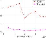
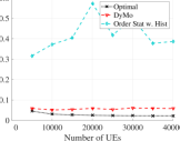
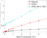
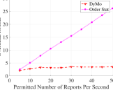
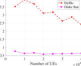
First, we consider the impact of changing these parameters on the accuracy of the SNR Threshold estimation. Figs. 10, 11, and 12 show the Root Mean Square Error (RMSE) in SNR Threshold percentile estimation vs. $m$, for homogeneous, stadium and failure scenarios, respectively. The non-zero values of RMSE in Optimal are due to quantization of SNR reports. The RMSE in the SNR Threshold estimation of DyMo is close to that of Optimal regardless of the number of UEs, while Order-Statistics w. History suffers from order of magnitude higher RMSE.

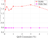
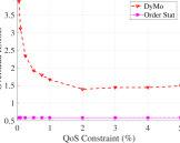
Figs. 10, 11, and 12 show the RMSE in SNR Threshold estimation as the QoS Constraint $p$ changes, for homogeneous, stadium and failure scenarios. DyMo outperforms the alternative schemes as $p$ increases. As $p$ increases, we observe an increasing quantization error, which impacts the RMSE of all the schemes including the Optimal. Recall that the SNR distribution is represented by a histogram where each bar has a width of $0.1dB$. As $p$ increases, the number UEs in the bar that contains the $p$ percentile UE increases as well. Since $s(t)$ should be below the SNR value of this bar, we notice a higher quantization error.

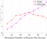
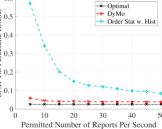
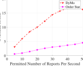
Figs. 10, 11, and 12 illustrate the SNR Threshold percentile RMSE as the Overhead Constraint is relaxed, for homogeneous, stadium and failure cases, respectively. The SNR Threshold percentile RMSE of DyMo is $0.05\%$ even with Overhead Constraint of $5$ reports/sec, while Optimal RMSE due to quantization is $0.025\%$. DyMo error slightly reduces by relaxing the Overhead Constraint (Optimal error stays $0.25\%$). Even with $10$ times higher reporting rate, DyMo significantly outperforms the Order-Statistics alternatives. The RMSE in SNR Threshold percentile for Order-Statistics is in the order of the required average value of $0.1$ even with a permitted overhead of $50$ reports/sec, i.e,. $3000$ reports per reporting interval. This is a very high overhead on the unicast traffic, since in LTE networks the number of simultaneously open unicast connections is limited, i.e., several hundreds per base station and each connection lasts several hundred msecs even for sending a short update. Unlike the downlink, uplink resources are not reserved for eMBMS systems and utilize the unicast resources. The RMSE of number of outliers is qualitatively similar to the SNR Threshold percentile results.

We also compute the overhead RMSE for different UE population sizes, $m$, QoS Constraint $p$, and Overhead Constraints $r$. The results are shown is sub-figures (d), (e) and (f) of Figs. 10, 11 and 12, respectively. In most cases, the overhead RMSE of DyMo is between $1-4$ even when the system parameters change. We observe an increase in the overhead RMSE only in failure scenarios when the permitted overhead is relaxed, as shown in Fig. 12. This is expected immediately after a failure because many more UEs suffer from poor service than DyMo estimated. Thus, as the permitted overhead increases also the spike in the number of reports during the first reporting interval after the failure also increases, which results in a gradual increase of the Overhead RMSE.

Figs. 10 and 12 show that the Order-Statistics variants experience very low violation of the Overhead Constraint in the homogeneous and Failure scenarios. This is not surprising, since in these scenarios the variation in the number of active eMBMS receivers is very small and this number is roughly $\operatorname*{\mathbb{E}}[m(t)]$ (the expected number of active eMBMS receivers). As mentioned in Section VI-A, this observation is misleading, since we assume that $\operatorname*{\mathbb{E}}[m(t)]$ is known and we ignore the overhead of configuring the UEs with the proper reporting rate. Obviously, the exact number of active receivers, $\operatorname*{\mathbb{E}}[m(t)]$, is unknown in practice. Furthermore, Fig. 11 shows that in scenarios with high variation in the number of active receivers, $m(t)$, (like the case in the stadium simulations) the violation of the Overhead Constraint is high and it is amplified as the permitted number of reports, $r$, increases. This is due to the static reporting rate of Order-Statistics despite dynamic changes of the number of active eMBMS receivers. Fig. 11 confirms that the overhead violation of Order-Statistics is very sensitive to the estimation of $\operatorname*{\mathbb{E}}[m(t)]$ and its variance.

Given that the number of active eMBMS receivers, $m(t)$, is unknown and may change significantly over time, Order-Statistics cannot practically preserve the Overhead Constraint without keeping track of the active UEs and sending individual messages to a subset of the active UEs. However, keeping track of $m(t)$ requires each UE to report when it starts and stops receiving eMBMS services, which may incur much higher overhead than permitted. For instance, in our simulations with $m=20,000$ UEs, even if such switching occurs at most once (start and stop) by each UE, the total number of reports is $40,000$. When dividing this number by the simulation duration of $30$ minutes ($1,800$ sec) we get $22$ messages/second, which is much higher than the permitted overhead.

Summary: Our simulations show that DyMo achieves accurate, close to optimal, estimation of the SNR Threshold even when the number of active eMBMS receivers is unknown. It can improve the spectral efficiency for eMBMS operation, while adding a very low reporting overhead. DyMo can predict the SNR Threshold with lower errors than other alternatives under a wide range of the SNR Threshold requirement $p$ and reporting Overhead Constraint $r$. These observations show that DyMo exceeds the expectations of our analysis in Section V.

VII Conclusion

This paper presents a Dynamic Monitoring (DyMo) system for large scale monitoring of eMBMS services, based on the concept of Stochastic Group Instructions. Our extensive simulations show that DyMo achieves accurate, close to optimal, estimation of the SNR Threshold even when the number of active UEs is unknown. It can improve the spectral efficiency for eMBMS operation while adding a low reporting overhead.

VIII Acknowledgment

This work was supported in part by NSF grants CNS-16-50669 and CNS-14-23105.

-A Analysis of the Two-Step Estimation Algorithm

We now extend the analysis of the Two-step estimation algorithm given in Section V-B. We show that the optimal settings for minimizing the error $\epsilon$ of Equation (3) is obtained by taking

$$p_{1}\!=\!p_{2}\!=\!\sqrt{p}~{}~{}~{}and~{}~{}~{}r_{1}\!=\!r_{2}\!=\!r/2$$

Notice that the settings should satisfy the following two constraints:

$$p=p_{1}\cdot p_{2}$$ (7)

and

$$r=r_{1}+r_{2}$$ (8)

From Equation (2) and by taking $3$ times the standard deviation, we get that the errors $\epsilon_{1}$ and $\epsilon_{2}$ are

$$\epsilon_{1}=3\sqrt{\frac{p_{1}(1-p_{1})}{r_{1}}}~{}~{}~{}and~{}~{}~{}\epsilon_{2}=3\sqrt{\frac{p_{2}(1-p_{2})}{r_{2}}}$$

By combining with Equation (3), we get

$$\epsilon=3\ \sqrt{\frac{p_{1}(1-p_{1})}{r_{1}}}\ p_{2}+3\ \sqrt{\frac{p_{2}(1-p_{2})}{r_{2}}}\ p_{1}$$ (9)

By using the two constraints (7) and (8), we assign $p_{2}=p/p_{1}$ and $r_{2}=r-r_{1}$. Consequently,

$$\begin{split}\epsilon=\ &3\ \sqrt{\frac{p_{1}(1-p_{1})}{r_{1}}}\ \frac{p}{p_{1}}+3\ \sqrt{\frac{(p/p_{1})(1-p/p_{1})}{r-r_{1}}}\ p_{1}\\ =\ &3\ p\left[\sqrt{\left(\frac{1}{p_{1}}-1\right)\ \frac{1}{r_{1}}}\ +\sqrt{\left(\frac{p_{1}}{p}-1\right)\ \frac{1}{r-r_{1}}}\right]\end{split}$$ (10)

By taking the partial derivative $\frac{\partial{\epsilon}}{\partial{p_{1}}}$ we get,

$$\begin{split}\frac{\partial{\epsilon}}{\partial{p_{1}}}=3\ p&\left[-\left(2\ p_{1}^{2}\ \sqrt{\left(\frac{1}{p_{1}}-1\right)\ \frac{1}{r_{1}}}\right)^{-1}+\right.\\ &\ \ \left.\left(2\ p\ \sqrt{\left(\frac{p_{1}}{p}-1\right)\ \frac{1}{r-r_{1}}}\right)^{-1}\right]\end{split}$$ (11)

For minimizing the error we calculate $\frac{\partial{\epsilon}}{\partial{p_{1}}}=0$ and get that

$$p_{1}^{2}\ \sqrt{\left(\frac{1}{p_{1}}-1\right)\frac{1}{r_{1}}}=p\ \sqrt{\left(\frac{p_{1}}{p}-1\right)\ \frac{1}{r-r_{1}}}$$ (12)

By simple mathematical manipulations we get

$$p_{1}^{4}\ \left(\frac{1}{p_{1}}-1\right)\left(r-r_{1}\right)=p^{2}\ \left(\frac{p_{1}}{p}-1\right)\ r_{1}$$ (13)

Similarly, from the partial derivative $\frac{\partial{\epsilon}}{\partial{r_{1}}}$ we get

$$\frac{\partial{\epsilon}}{\partial{r_{1}}}=3\ p\left[\sqrt{\left(\frac{1}{p_{1}}-1\right)}\ \frac{-1}{2\ r_{1}^{3/2}}+\sqrt{\left(\frac{p_{1}}{p}-1\right)}\ \frac{1}{2\ (r-r_{1})^{3/2}}\right]$$ (14)

For minimizing the error we calculate $\frac{\partial{\epsilon}}{\partial{r_{1}}}=0$ and get that

$$\sqrt{\left(\frac{1}{p_{1}}-1\right)}\ \frac{1}{2\ r_{1}^{3/2}}=\sqrt{\left(\frac{p_{1}}{p}-1\right)}\ \frac{1}{2\ (r-r_{1})^{3/2}}$$ (15)

By simple mathematical manipulations we get

$$\left(\frac{1}{p_{1}}-1\right)\ \left(r-r_{1}\right)^{3}=\left(\frac{p_{1}}{p}-1\right)\ r_{1}^{3}$$ (16)

Noticed that Equations (13) and (16) together provide two simple conditions to optimize $p_{1}$ and $r_{1}$. By dividing Equation (13) by Equation (16) we obtain,

$$\left(r-r_{1}\right)=\frac{r_{1}\ p_{1}^{2}}{p}$$ (17)

Using Equation (17) in Equation (16) results that

$$\begin{split}\left(\frac{1}{p_{1}}-1\right)\ \left(\frac{r_{1}\ p_{1}^{2}}{p}\right)^{3}=&\left(\frac{p_{1}}{p}-1\right)\ r_{1}^{3}\\ \left(\frac{1}{p_{1}}-1\right)\ \frac{p_{1}^{6}}{p^{2}}=&\left(\frac{p_{1}}{p}-1\right)\end{split}$$ (18)

From this we get the following relation

$$p_{1}^{6}-p_{1}^{5}+p_{1}\ p^{2}-p^{3}=0$$ (19)

The only real solutions are $p_{1}=\pm\sqrt{p}$. Since $p_{1}$ must be positive we get that $p=\sqrt{p}$. From this solution and Equation (17), it is implies that the optimal setting is

$$p_{1}=p_{2}=\sqrt{p},~{}~{}and~{}~{}r_{1}=r_{2}=r/2$$

Consequently, the errors of the two steps are

$$\epsilon_{1}\!=\!\epsilon_{2}\!=\!3\sqrt{\sqrt{p}(1-\sqrt{p})/(r/2)}$$

From this we obtain Proposition 1 and a bound on the error of,

$$6\sqrt{2}\sqrt{\frac{p\sqrt{p}(1-\sqrt{p})}{r}}$$

This concludes our analysis of the Two-step estimation algorithm.

References

- [1] J. Erman and K. K. Ramakrishnan, “Understanding the super-sized traffic of the super bowl.,” in Proc. ACM IMC’13, 2013.
- [2] Y. Tanigawa, K. Yasukawa, and K. Yamaoka, “Transparent unicast translation to improve quality of multicast over wireless LAN,” in Proc. IEEE CCNC’10, 2010.
- [3] A. Kaya, D. Calin, and H. Viswanathan, “On the performance of stadium high density carrier Wi-Fi enabled LTE small cell deployments,” in Proc. IEEE WCNC’15, 2015.
- [4] “3GPP TS 26.346 V13.1.0, 3rd Generation Partnership Project; Technical Specification Group Services and System Aspects; Multimedia Broadcast/Multicast Service (MBMS); Protocols and codecs (Release 13),” June 2015.
- [5] D. Lecompte and F. Gabin, “Evolved multimedia broadcast/multicast service (eMBMS) in LTE-advanced: overview and rel-11 enhancements,” IEEE Comm. Mag., vol. 50, no. 11, pp. 68–74, 2012.
- [6] “3GPP TS 37.320 V12.2.0 , 3rd Generation Partnership Project; Technical Specification Group Radio Access Network; Universal Terrestrial Radio Access (UTRA) and Evolved Universal Terrestrial Radio Access (E-UTRA); Radio measurement collection for Minimization of Drive Tests (MDT); Overall description; Stage 2 (Release 12),” Sept. 2014.
- [7] J. Vella and S. Zammit, “A survey of multicasting over wireless access networks,” IEEE Commun. Surv. & Tut., vol. 15, no. 2, pp. 718–753, 2013.
- [8] V. Gupta, Y. Bejerano, C. Gutterman, J. Ferragut, K. Guo, T. Nandagopal, and G. Zussman, “Light-weight feedback mechanism for WiFi multicast to very large groups - experimental evaluation,” IEEE Trans. Netw. (to appear), 2016.
- [9] X. Wang, L. Wang, and D. Wang, Y.and Gu, “Reliable multicast mechanism in WLAN with extended implicit MAC acknowledgment,” in Proc. IEEE VTC’08, 2008.
- [10] Z. Feng, G. Wen, C. Yin, and H. Liu, “Video stream groupcast optimization in WLAN,” in Proc. IEEE ITA’10, 2010.
- [11] Y. Cai, S. Lu, L. Zhang, C. Wang, P. Skov, Z. He, and K. Niu, “Reduced feedback schemes for LTE MBMS,” in Proc. IEEE VTC’09, 2009.
- [12] A. B. Owen, Monte Carlo theory, methods and examples. 2013.
- [13] D. Lecompte and F. Gabin, “Evolved multimedia broadcast/multicast service (eMBMS) in LTE-advanced: overview and Rel-11 enhancements,” IEEE Commun. Mag., vol. 50, no. 11, 2012.
- [14] J. Yoon, H. Zhang, S. Banerjee, and S. Rangarajan, “MuVi: a multicast video delivery scheme for 4G cellular networks,” in Proc. ACM MOBICOM’11, 2012.
- [15] R. Sivaraj, A. Pande, and P. Mohapatra, “Spectrum-aware radio resource management for scalable video multicast in LTE-advanced systems,” in Proc. IFIP Networking’13, 2013.
- [16] L. Militano, D. Niyato, M. Condoluci, G. Araniti, A. Iera, and G. M. Bisci, “Radio resource management for group-oriented services in LTE-A,” IEEE Trans. Veh. Technol., vol. 64, no. 8, pp. 3725–3739, 2015.
- [17] J. Chen, M. Chiang, J. Erman, G. Li, K. Ramakrishnan, and R. K. Sinha, “Fair and optimal resource allocation for LTE multicast (eMBMS): group partitioning and dynamics,” in Proc. IEEE INFOCOM’15, 2015.
- [18] F. Wu, Y. Yang, O. Zhang, K. Srinivasan, and N. B. Shroff, “Anonymous-query based rate control for wireless multicast: Approaching optimality with constant feedback,” in Proc. ACM MOBIHOC ’16, 2016.
- [19] J. Villalon, P. Cuenca, L. Orozco-Barbosa, Y. Seok, and T. Turletti, “Cross-layer architecture for adaptive video multicast streaming over multirate wireless LANs,” IEEE J. Sel. Areas Commun., vol. 25, no. 4, pp. 699–711, 2007.
- [20] R. Chandra, S. Karanth, T. Moscibroda, V. Navda, J. Padhye, R. Ramjee, and L. Ravindranath, “DirCast: a practical and efficient Wi-Fi multicast system,” in Proc. IEEE ICNP’09, 2009.
- [21] S. Sen, N. K. Madabhushi, and S. Banerjee, “Scalable WiFi media delivery through adaptive broadcasts,” in Proc. USENIX NSDI’10, 2010.
- [22] V. Gupta, C. Gutterman, Y. Bejerano, and G. Zussman, “Dynamic rate adaptation for WiFi multicast to very large groups – design and experimental evaluation,” in Proc. IEEE INFOCOM’16, 2016.
- [23] A. Silberschatz, H. F. Korth, and S. Sudarshan, Database System Concepts, Sixth Edition. McGraw-Hill, 2010.
- [24] A. W. Van der Vaart, Asymptotic statistics. Cambridge university press, 2000.
- [25] I. Rhee, M. Shin, S. Hong, K. Lee, S. J. Kim, and S. Chong, “On the levy-walk nature of human mobility,” IEEE Trans. Netw., vol. 19, no. 3, pp. 630–643, 2011.
- [26] S. Scellato, I. Leontiadis, C. Mascolo, P. Basu, and M. Zafer, “Evaluating temporal robustness of mobile networks,” IEEE Trans. Mobile Comput., vol. 12, no. 1, pp. 105–117, 2013.