Identifying Best Interventions through Online Importance Sampling

Abstract

Motivated by applications in computational advertising and systems biology, we consider the problem of identifying the best out of several possible soft interventions at a source node $V$ in an acyclic causal directed graph, to maximize the expected value of a target node $Y$ (located downstream of $V$). Our setting imposes a fixed total budget for sampling under various interventions, along with cost constraints on different types of interventions. We pose this as a best arm identification bandit problem with $K$ arms where each arm is a soft intervention at $V,$ and leverage the information leakage among the arms to provide the first gap dependent error and simple regret bounds for this problem. Our results are a significant improvement over the traditional best arm identification results. We empirically show that our algorithms outperform the state of the art in the Flow Cytometry data-set, and also apply our algorithm for model interpretation of the Inception-v3 deep net that classifies images.

1 Introduction

Causal graphs [28] are useful for representing causal relationships among interacting variables in large systems [7]. Over the last few decades, causal models have found use in computational advertising [7], biological systems [25], sociology [5], agriculture [36] and epidemiology [18]. There are two important questions commonly studied with causal graphs: (i) How to learn a directed causal graph that encodes the pattern of interaction among components in a system (casual structure learning)? [28] , and (ii) Using previously acquired (partial) knowledge about the causal graph structure, how to estimate and/or to optimize the effect of a new intervention on other variables (optimization) [7, 18, 20, 6, 21]? Here, an intervention is a forcible change to the value of a variable in a system. The change either alters the relationship between the parental causes and the variable, or decouples it from the parental causes entirely. Our focus is on optimizing over a given set of interventions.

Figure 1: Computational advertising example borrowed from [7]. Various observable and hidden variables are shown. The topology of the causal graph is known; however the strengths of most interactions are unknown. A click-rate scoring algorithm predicts future user click through rates from users’ search queries and the set of ads relevant to the user query chosen from an ad inventory. The algorithm’s output determines the ads displayed (as well as the display style), and through a complex causal graph, finally determines actual revenue. The part of the network in bold – distribution of user queries and matching ad keywords is known (including strengths), and the input output characteristics of several candidate (randomized) click-rate scoring algorithms are known. The objective is to choose the best algorithm that maximizes the revenue (target in bold red).

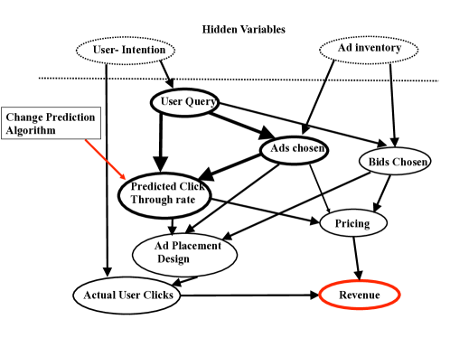
An illustrative example includes online advertising [7], where there is a collection of click-through rate scoring algorithms that provide an estimate of the probability that an user clicks on an ad displayed at a specific position. The interventions occur through the choice of click-through rate scoring algorithm; the algorithm choice directly impacts ad placement and pricing, and through a complex network of interactions, affects the revenue generated through advertisements. The revenue is used to determine the best scoring algorithm (optimize for the best intervention); see Figure 1. Another example is in biological gene-regulatory networks [6], where a large number of genomes interact amongst each other and also interact with environmental factors. The objective here is to understand the best perturbation of some genomes in terms of its effect on the expression of another subset of genomes (target) in cellular systems.

This paper focuses on the following setting: We are given apriori knowledge about the structure and strength of interactions over a small part of the causal graph. In addition, there is freedom to intervene (from a set of allowable interventions) at a certain node in the known part of the graph, and collect data under the chosen intervention; further we can alter the interventions over time and observe the corresponding effects. Given a set of potential interventions to optimize over, the key question of interest is: How to choose the best sequence of $T$ allowable interventions in order to discover which intervention maximizes the expectation of a downstream target node?

Determining the best intervention in the above setting can be cast as a best arm identification bandit problem, as noted in [22]. The possible interventions to optimize over are the arms of the bandit, while the sample value of the target node under an intervention is the reward.

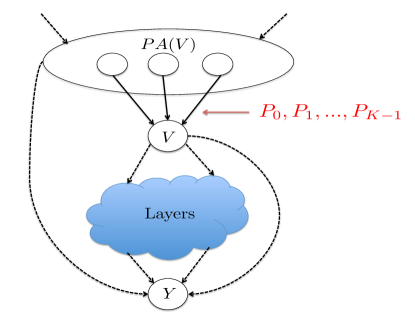
More formally, suppose that $V$ is a node in a causal graph $\mathcal{G}(\mathcal{V},\mathcal{E})$ (as shown in Fig. 2), with the parents of $V$ denoted by $pa(V).$ In Fig. 1, $V$ corresponds to the click-through rate and its parents are user-query and ads-chosen. This essentially means that $V$ is causally determined by a function of $pa(V)$ and some exogenous random noise. This dependence is characterized by the conditional $\mathrm{P}(V|pa(V))$. Then a (soft) intervention mathematically corresponds to changing this conditional probability distribution i.e. probabilistically forcing $V$ to certain states given its parents. In the computational advertising example, the interventions correspond to changing the click through rate scoring algorithm i.e $\mathrm{P}(click~{}through~{}rate|ads~{}chosen,user~{}query)$, whose input-output characteristics are well-studied. Further, suppose that the effect of an intervention is observed at a node $Y$ which is downstream of $V$ in the topological order (w.r.t $\mathcal{G}$) -refer to Fig. 2. Then, our key question is stated as follows: Given a collection of interventions $\{\mathrm{P}_{0}(V|pa(V)),\ldots\mathrm{P}_{K-1}(V|pa(V))\},$ find the best intervention among these $K$ possibilites that maximizes $E[Y]$ under a fixed budget of $T$ (intervention, observation) pairs.

Figure 2: Illustration of our setting. The soft interventions modify $\mathrm{P}(V|pa(V)$. The various conditionals and the marginal of $pa(V)$ is assumed to be known from prior data. The target variable $Y$ lies further downstream in the unknown portions of the causal graph.

1.1 Main Contributions

(Successive Rejects Algorithm) We provide an efficient successive rejects multi-phase algorithm. The algorithm uses clipped importance sampling. The clipper level is set adaptively in each phase in order to trade-off bias and variance. Our procedure yields a major improvement over the algorithm in [22] (both in theoretical guarantees and in practice), which sets the clippers and allocates samples in a static manner.

(Gap Dependent Error Guarantees under Budget Constraints) In the classic best arm identification problem [3], Audibert et al. derive gap dependent bounds on the probability of error given a fixed sample budget. Specifically, let $\Delta_{(i)}$ be the $i$-th largest gap (difference) in the expected reward from that of the best arm (e.g. $\Delta_{(1)}$ is the difference between the best arm expected reward and the second best reward). Then, it has been shown in [3] that the number of samples needed scales as (upto poly log factors) $\max_{i}(i/\Delta_{(i)}^{2}).$

In our setting, a fundamental difference from the classical best arm setting [3] is the information leakage across the arms, i.e, samples from one arm can inform us about the expected value of other arms because of the shared causal graph. We show that this information leakage yields significant improvement both in theory and practice. We derive the first gap dependent (gaps between the expected reward at the target under different interventions) bounds on the probability of error in terms of the number of samples $T$, cost budget $B$ on the relative fraction of times various arms are sampled and the divergences between soft intervention distributions of the arms.

In our result (upto poly log factors) the factor $i$ is replaced by the ’effective variance’ of the estimator for arm $(i)$, i.e. we obtain (with informal notation) $\max_{i}\sigma_{i}^{2}/\Delta_{(i)}^{2}$. $\sigma_{i}$ can be much smaller than $\sqrt{i}$ (the corresponding term in the results of [3]). Our theoretical guarantees quantify the improvement obtained by leveraging information leakage, which has been empirically observed in [7]. We discuss in more detail in Sections 3.3 and B (in the appendix), about how these guarantees can be exponentially better than the classical ones. We derive simple regret (refer to Section 3.1) bounds analogous to the gap dependent error bounds.

(Novel $f$-divergence measure for analyzing Importance Sampling) We provide a novel analysis of clipped importance sampling estimators, where pairwise $f$-divergences between the distributions $\{\mathrm{P}_{k}(V|pa(V))\}$, for a carefully chosen function $f(.)$ (see Section C.1) act as the ‘effective variance’ term in the analysis for the estimators (similar to Bernstein’s bound [4]).

(Extensive Empirical Validation) We demonstrate that our algorithm outperforms the prior works [22, 3] on the Flow Cytometry data-set [32] (in Section 4.1). We exhibit an innovative application of our algorithm for model interpretation of the Inception Deep Network [38] for image classification (refer to Section 4.2).

Remark 1.

The techniques in this paper can be directly applied to more general settings like (i) the intervention source ($V$) can be a collection of nodes ($\mathcal{V}$) and the changes affect the distribution $P(\mathcal{V}|pa(\mathcal{V}))$, where $pa(\mathcal{V})$ is the union of all the parents; (ii) the importance sampling can be applied at a directed cut separating the sources and the targets, provided the effect of the interventions, on the nodes forming the cut can be estimated. Moreover, our techniques can be applied without the complete knowledge of the source distributions. We explain the variations in more detail in Section A in the appendix.

1.2 Related Work

The problem lies at the intersection of causal inference and best arm identification in bandits. There have been many studies on the classical best arm identification in the bandit literature, both in the fixed confidence regime [19, 13] and in the fixed budget setting [3, 10, 17, 8]. It was shown recently in [8] that the results of [3] are optimal. The key difference from our work is that, in these models, there is no information leakage among the arms.

There has been a lot of work [27, 16, 12, 15, 35, 29, 24, 33] on learning casual models from data and/or experiments and using it to estimate causal strength questions of the counterfactual nature. One notable work that partially inspired our work is [7] where the causal graph underlying a computational advertising system (like in Bing, Google etc.) is known and the primary interest is to find out how a change in the system would affect some other variable.

At the intersection of causality and bandits, [22] is perhaps most relevant to our setting. It studies the problem of identifying the best hard interventions on multiple variables (among many), provided the distribution of the parents of the target is known under those interventions. Simple regret bound of order $O(1/\sqrt{T})$ was derived. We assume soft interventions that affect the mechanism between a ’source’ node and its parents, far away from the target (similar to the case of computational advertising considered in [7]). Further, we derive the first gap dependent bounds (that can be exponentially small in $T$), generalizing the results of [3]. Our formulation can handle general budget constraints on the bandit arms and also recover the problem independent bounds of [22] (orderwise). Budget constraints in bandit settings have been explored before in [1, 34].

In the context of machine learning, importance sampling has been mostly used to recondition input data to adhere to conditions imposed by learning algorithms [37, 23, 39].

2 Problem Setting

A causal graph $\mathcal{G}(\mathcal{V},\mathcal{E})$ specifies causal relationships among the random variables representing the vertices of the graph $\mathcal{V}$. The relationships are specified by the directed edges $\mathcal{E}$; an edge $V_{i}\rightarrow V_{j}$ implies that $V_{i}\in\mathcal{V}$ is a direct parental cause for the effect $V_{j}\in\mathcal{V}$. With some abuse of notation, we will denote the random variable associated with a node $V\in\mathcal{V}$ by $V$ itself. We will denote the parents of a node $V$ by $pa(V)$. The causal dependence implies that $V=f_{V}({U\in pa(V)},\epsilon_{V})$, where $\epsilon_{V}$ is an independent exogenous noise variable. One does not get to measure the functions $f_{V}$ in practice. The noise variable and the above functional dependence induce a conditional probability distribution $\mathrm{P}(V|pa(V))$. Further, the joint distribution of $\{V\}_{V\in\mathcal{V}}$ decomposes into product of conditional distributions according to $\mathcal{G}$ viewed as a Bayesian Network, i.e. $\mathrm{P}(\{V\}_{V\in\mathcal{V}})=\prod\limits_{V\in\mathcal{V}}\mathrm{P}(V|pa(V))$.

Interventions in a causal setting can be categorized into two kinds:

1. Soft Interventions: At node $V$, the conditional distribution relating $pa(V)$ and $V$ is changed to $\tilde{\mathrm{P}}\left(V|pa(V)\right)$.

2. Hard Interventions: We force the node $V$ to take a specific value $x$. The conditional distribution $\tilde{\mathrm{P}}\left(V|pa(V)\right)$ is set to a point mass function $\mathbf{1}_{V=x}$.

In this work, we consider the problem of identifying the best soft intervention, i.e. the one that maximizes the expected value of a certain target variable. The problem setting is best illustrated in Figure 2. Consider a causal graph $\mathcal{G}(\mathcal{V},\mathcal{E})$ that specifies directed causal relationships between the variables $\mathcal{V}$. Let $Y$ be a target random variable which is downstream in the graph $\mathcal{G}$; the expected value of this target variable is the quantity of interest. Consider another random variable $V$ along with its parents $pa(V)$. We assume that there are $K$ possible soft interventions. Each soft intervention is a distinct conditional distribution that dictates the relationship $pa(V)\rightarrow V$. During a soft intervention $k\in[K]$ ($[K]=\{0,1,...,K-1\}$), the conditional distribution of $V$ given its parents is set to $\mathrm{P}_{k}(V|pa(V))$ and all other relationships in the causal graph are unchanged.

It is assumed that the conditional distributions $\mathrm{P}_{k}(V|pa(V))$ and marginals for $pa(V)$ for $k\in[K]$ are known from past experiments or existing domain knowledge. We only observe samples of $Y,V$ and $pa(V)$, while the rest of the variables in the causal graph may be unobserved under different interventions. For simplicity we assume that the variables $V,pa(V)$ are discrete while the target variable $Y$ may be continuous/discrete and has bounded support in $[0,1]$. Further, we assume that the various conditionals, i.e. $\mathrm{P}_{k}\left(V|pa(V\right))$ are absolutely continuous with respect to each other. In the case of discrete distributions, the non-zero supports of these distributions are identical. However, our algorithm can be easily generalized for continuous distributions on $V$ and $pa(V)$ (as in our experiments in Section 4.1). In this setting, we are interested in the following natural questions: Which of the $K$ soft interventions yield the highest expected value of the target $(\mathbb{E}[Y])$ and what is the misidentification error that can be achieved with a finite total budget $T$ for samples ?

Remark 2.

Although we may know apriori the joint distribution of $pa(V)$ and $V$ under different interventions, how the change affects another variable $Y$ in the causal graph is unknown and must be learnt from samples. The task is to transfer prior knowledge to identify the best intervention.

Bandit Setting: The $K$ different soft interventions can be thought of as the $K$ arms of a bandit problem. Let the reward of arm $k$ be denoted by: $\mu_{k}={\mathbb{E}}_{k}\left[Y\right]$, where ${\mathbb{E}}_{k}\left[Y\right]$ is the expected value of $Y$ under the soft intervention when the conditional distribution of $V$ given its parents $pa(V)$ is set to $\mathrm{P}_{k}(V|pa(V))$ (soft intervention $k$) while keeping all other things in $\mathcal{G}$ unchanged. We assume that there is only one best arm. Let $k^{*}$ be the arm that yields the highest expected reward and $\mu^{*}$ be the value of the corresponding expected reward i.e. $k^{*}=\operatorname*{arg\,max}_{k}\mu_{k}$ and $\mu^{*}=\mu_{k^{*}}.$ Let the optimality gap of the $k^{th}$ arm be defined as $\Delta_{k}=\mu^{*}-\mu_{k}$. We shall see that the these gaps $\{\Delta_{k}\}_{k=0}^{K-1}$ and the relationship between distributions $\{\mathrm{P}_{k}(V|pa(V))\}_{k=0}^{K-1}$ are important parameters in the problem. Let the minimum gap be $\Delta=\min_{k\neq k^{*}}\Delta_{k}$.

Fixed Budget for Samples: In this paper, we work under the fixed budget setting of best arm identification [3]. Let $T_{k}$ be the number of times the $k^{th}$ intervention is used to obtain samples. We require that $\sum_{k=0}^{K}T_{k}=T$. Let $\nu_{k}=\frac{T_{k}}{T}$ be the fraction of times the $k^{th}$ intervention is played.

Additional Cost Budget on Interventions: In the context of causal discovery, some interventions require a lot more resources or experimental effort than the others. We find such examples in the context of online advertisement design [7]. Therefore, we introduce two variants of an additional cost constraint that influences the choice of interventions. (i) Difficult arm budget (S1): Some arms are deemed to be difficult. Let $\mathcal{B}\subset[K]$ be the set of difficult arms. We require that the total fraction of times the difficult arms are played does not exceed $B$ i.e. $\sum_{k\in\mathcal{B}}\nu_{k}\leq B.$ (ii) Cost Budget (S2): This is the most general budget setting that captures the variable costs of sampling each arm [34]. We assume that there is a cost $c_{k}$ associated with sampling arm $k$. It is required that the average cost of sampling does not exceed a cost budget $B$ .ie. $\sum_{k=0}^{K-1}c_{k}\nu_{k}\leq B.$ $\mathbf{c}=[c_{1},..,c_{k}]$ along with the total budget $T$ completely defines this budget setting. It should be noted that S1 is a special case of S2.

We note that unless otherwise stated, we work with the most general setting in S2. We state some of our results in the setting S1 for clearer exposition.

Objectives: There are two main quantities of interest:

(Probability of Error): This is the probability of failing to identify the best soft intervention (arm). Let $\hat{k}(T,B)$ be the arm that is predicted to be the best arm at the end of the experiment. Then the probability of error $e(T,B)$ [3, 8] is given by,

$e(T,B)={\mathbb{P}}\left(\hat{k}(T,B)\neq k^{*}\right)$

(Simple Regret): Another important quantity that has been analyzed in the best arm identification setting is the simple regret [22]. The simple regret is given by $r(T,B)=\sum_{k\neq k^{*}}\Delta_{k}{\mathbb{P}}\left(\hat{k}(T,B)=k\right)$.

3 Our Main Results

In this section we provide our main theoretical contributions. In Section 2, we provide a successive rejects style algorithm that leverages the information leakage between the arms via importance sampling. Then, we provide theoretical guarantees on the probability of mis-identification $(e(T,B))$ and simple regret $(r(T,B))$ for our algorithm in Section 3.3. In order to explain our algorithm and our results formally, we first describe several key ideas in our algorithm and introduce important definitions in Section 3.1.

3.1 Definitions

Quantifying Information Leakage: Our setting is one in which there is information leakage among the $K$ arms of the bandit. Recall that each arm corresponds to a different conditional distribution imposed on a node $V$ given its parents $pa(V)$, while the rest of the relationships in the causal graph $\mathcal{G}$ remain unchanged. Since the different candidate conditional distributions $\mathrm{P}_{k}(V|pa(V))$ are known from prior knowledge (and are absolutely continuous with respect to each other), it is possible to utilize samples obtained under an arm $j$ to obtain an estimate for the expectation under some other arm $i$ (i.e ${\mathbb{E}}_{i}\left[Y\right]$). A popular method for utilizing this information leakage among different distributions is through importance sampling, which has been used in counterfactual analysis in similar causal settings [22, 7].

Importance Sampling: Suppose we get samples from arm $j\in[K]$ and we are interested in estimating ${\mathbb{E}}_{i}[Y]$. In this context it helpful to express ${\mathbb{E}}_{i}[Y]$ in the following manner:

$${\mathbb{E}}_{i}\left[Y\right]={\mathbb{E}}_{j}\left[Y\frac{\mathrm{P}_{i}(V|pa(V))}{\mathrm{P}_{j}(V|pa(V))}\right]$$ (1)

(1) is trivially true because the only change to the joint distribution of all the variables in the causal graph $\mathcal{G}$ under arm $i$ and $j$ is at the factor $\mathrm{P}(V|pa(V))$. Suppose we observe $t$ samples of $\{Y,V,pa(V)\}$ from the arm $j$, denoted by $\{Y_{j}(s),V_{j}(s),pa(V)_{j}(s)\}_{s=1}^{t}$. Here $X_{j}(s)$ denotes the sample from random variable $X$ at time step $s$, while the sub-script $j$ just denotes that the samples are collected under arm $j$. Under the observation of Equation (1), one might assume that the naive estimator,

$$\hat{Y}^{\prime}_{i}(j)=\frac{1}{t}\sum_{s=1}^{t}Y_{j}(s)\frac{\mathrm{P}_{i}(V_{j}(s)|pa(V)_{j}(s))}{\mathrm{P}_{j}(V_{j}(s)|pa(V)_{j}(s))}$$ (2)

provides a good estimate for $\mu_{i}={\mathbb{E}}_{i}\left[Y\right]$. However, the confidence guarantees on such an estimate can be arbitrarily bad even if $Y$ is bounded. This is because the factor $\mathrm{P}_{i}(V|pa(V))/\mathrm{P}_{j}(V|pa(V))$ can be very large for several instances of $(V,pa(V))$. Therefore, usual measure concentrations (e.g. the Azuma-Hoeffding inequality) would not yield good confidence intervals. This has been noted in [22] in a similar setting, where a static clipper has been applied to the weighted samples to control the variance. However, a static clipper introduces a fixed bias, and thus it is not suitable for obtaining gap dependent simple regret bounds. Instead, in our algorithm we a multi-phase approach and use dynamic clipping to adaptively control the bias vs. variance trade-off in a phase dependent manner, which leads to significantly better gap dependent bounds. We now define some key quantities.

Definition 1.

Let $f(\cdot)$ be a non-negative convex function such that $f(1)=0$. For two joint distributions $p_{X,Y}(x,y)$ and $q_{X,Y}(x,y)$ (and the associated conditionals), the conditional $f$-divergence $D_{f}(p_{X|Y}\|q_{X|Y})$ is given by:

$$D_{f}(p_{X|Y}\|q_{X|Y})={\mathbb{E}}_{q_{X,Y}}\left[f\left(\frac{p_{X|Y}(X|Y)}{q_{X|Y}(X|Y)}\right)\right].$$

Recall that $\mathrm{P}_{i}$ is the conditional distribution of node $V$ given the state of its parents $pa(V).$ Thus, $D_{f}(\mathrm{P}_{i}\|\mathrm{P}_{j})$ is the conditional $f$-divergence between the conditional distributions $P_{i}$ and $P_{j}.$ Now we define some log-divergences that are are crucial in the our analysis.

Definition 2.

($M_{ij}$ measure) Consider the function $f_{1}(x)=x\exp(x-1)-1$. We define the following log-divergence measure: $M_{ij}=1+\log(1+D_{f_{1}}(\mathrm{P}_{i}\lVert\mathrm{P}_{j})),$ $\forall i,j\in[K].$

These log divergences help us in controlling the bias variance trade-off in importance sampling as shown in Section C.2 in the appendix. We also note that estimates of the $f$-divergence measure can be had directly from empirical data (without the knowledge of the full distributions) using techniques like that of [30].

Aggregating Interventional Data: We describe an efficient estimator of ${\mathbb{E}}_{k}[Y]$ ($\forall k\in[K]$) that combines available samples from different arms. This estimator adaptively weights samples depending on the relative $M_{ij}$ measures, and also uses clipping to control variance by introducing bias. The estimator is given by (3).

Suppose we obtain $\tau_{i}$ samples from arm $i\in[K]$. Let the total number of samples from all arms be denoted by $\tau$. Further, let us index all the samples by $s\in\{1,2,..,\tau\},$ and $\mathcal{T}_{k}\subset\{1,2,..,\tau\}$ be the indices of all the samples collected from arm $k$. Let $X_{j}(s)$ denotes the sample collected for random variable $X$ under intervention $j$, at time instant $s$. Finally, let $Z_{k}=\sum_{j\in[K]}\tau_{j}/M_{kj}$. We denote the estimate of $\mu_{k}$ by $\hat{Y}_{k}^{\epsilon}$ ($\epsilon$ indicates the level of confidence desired). Our estimator is:

$$\hat{Y}_{k}^{\epsilon}=\frac{1}{Z_{k}}\sum_{j=0}^{K}\sum_{s\in\mathcal{T}_{j}}\frac{1}{M_{kj}}Y_{j}(s)\frac{\mathrm{P}_{k}(V_{j}(s)|pa(V)_{j}(s))}{\mathrm{P}_{j}(V_{j}(s)|pa(V)_{j}(s))}\times\mathds{1}\left\{\frac{\mathrm{P}_{k}(V_{j}(s)|pa(V)_{j}(s))}{\mathrm{P}_{j}(V_{j}(s)|pa(V)_{j}(s))}\leq 2\log(2/\epsilon)M_{kj}\right\}.$$ (3)

In other words, $\hat{Y}_{k}^{\epsilon}$ is the weighted average of the clipped samples, where the samples from arm $j$ are weighted by $1/M_{kj}$ and clipped at $2\log(2/\epsilon)M_{kj}$. The choice of $\epsilon$ controls the bias-variance tradeoff which we will adaptively change in our algorithm.

3.2 Algorithm

Now, we describe our main algorithmic contribution - Algorithm 1 and 2. Algorithm 1 starts by having all the $K$ arms under consideration and then proceeds in phases, possibly rejecting one or more arms at the end of each phase.

At every phase, Estimator $(\ref{eq:uniestimator_main})$ with a phase specific choice of the $\epsilon$ parameter (i.e. controlling bias variance trade-off), is applied to all arms under consideration. Using a phase specific threshold on these estimates, some arms are rejected at the end of each phase. A random arm among the ones surviving at the end of all phases is declared to be the optimal. We now describe the duration of various phases.

Recall the parameters $T$ - Total sample budget available and $B$ - average cost budget constraint. Let $n(T)=\lceil\log 2\times\log 10\sqrt{T}\rceil$. Let $\overline{\log}(n)=\sum_{i=1}^{n}(1/i)$. We will have an algorithm with $n(T)$ phases numbered by $\ell=1,2.,,n(T)$. Let $\tau(\ell)$ be the total number of samples in phase $\ell$. We set $\tau(l)=T/(l\overline{\log}(n(T)))$ for $l\in\{1,..,n(T)\}$. Note that $\sum_{l}\tau(l)=T$. Let ${\cal R}$ be the set of arms remaining to compete with the optimal arm at the beginning of phase $\ell$ which is continuously updated.

Allocation of Budget: Let $\tau_{k}(\ell)$ be the samples allocated to arm $k$ in phase $\ell$. Let $\boldsymbol{\tau(\ell)}$ be the vector consisting of entries $\{\tau_{k}\left(\ell\right)\}$. The vector of allocated samples, i.e. $\boldsymbol{\tau(\ell)}$ is decided by Algorithm 3. Intuitively, an arm that provides sufficient information about all the remaining arms needs to be given more budget than other less informative arms. This allocation depends on the average budget constraints and the relative log divergences between the arms (Definition 2). Algorithm 3 formalizes this intuition, and ensures that variance of the worst estimator (of the form (3)) for the arms in $\mathcal{R}$ is as good as possible (quantified in Theorem 4 and Lemma 4 in the appendix).

The inverse of the maximal objective of the LP in Algorithm 3 acts as effective standard deviation uniformly for all the estimators for the remaining arms in $\mathcal{R}$. It is analogous to the variance terms appearing in Bernstein-type concentration bounds (refer to Lemma 4 in the appendix).

Definition 3.

The effective standard deviation for budget $B$ and arm set ${\cal R}\subseteq[K]$ is defined as ${\sigma^{*}(B,{\cal R})}=1/v^{*}(B,{\cal R})$ from Algorithm 3 with input $B$ and arm set ${\cal R}$.

Algorithm 3 minimizes the variance terms in the confidence bounds for the estimates of the arms that are in contention i.e. $\hat{Y}_{k}^{\epsilon}$ for all $k\in\mathcal{R}$. This minimization is performed subject to the constraints on the fractional budget of each arms (recall $B$ from Section 2). Note that Algorithm 3 only needs to ensure good confidence bounds for the arms that are remaining ($k\in\mathcal{R}$). This gets easier as the number of arms remaining (i.e. $\lvert\mathcal{R}\rvert$) decreases. Therefore the effective variances $\sigma^{*}(B,{\cal R})$ become progressively better with every phase.

Algorithm 1 Successive Rejects with Importance Sampling -v1 (SRISv1) - Given total budget $T$ and the cost budget $B$ (along with $c_{i}$’s) picks the best arm.

1:  $\mathrm{SRIS}(B,\{M_{kj}\},T)$

2:  ${\cal R}=[K]$.

3:  Form the matrix $\mathbf{A}\in\mathbb{R}^{K\times K}$ such that $A_{kj}=\frac{1}{M_{kj}}$.

4:  for $\ell=1$ to $n(T)$ do

5:     $\boldsymbol{\tau(\ell)}=\mathrm{ALLOCATE}\left(\mathbf{c},B,\mathbf{A},{\cal R},\tau(\ell)\right)$ (Algorithm 3)

6:     Use arm $k$, $\tau_{k}(\ell)$ times and collect samples $(Y,V,pa(V))$.

7:     for $k\in{\cal R}$ do

8:        Let $\hat{Y}_{k}$ be the estimator for arm $k$ as in (3) calculated with $\{M_{kj}\}$, $\epsilon=2^{-(\ell-1)}$ and the samples obtained in Line 6.

9:     end for

10:     Let $\hat{Y}_{H}=\operatorname*{arg\,max}_{k\in{\cal R}}\hat{Y}_{k}$.

11:     ${\cal R}={\cal R}-\{k\in{\cal R}:\hat{Y}_{H}>\hat{Y}_{k}+5/2^{l}\}$.

12:     if $\lvert{\cal R}\rvert=1$ then

13:        return: the arm in ${\cal R}$.

14:     end if

15:  end for

16:  return: A randomly chosen arm from ${\cal R}$.

Remark 3.

Note that Line 6 uses only the samples acquired in that phase. Clearly, a natural extension is to modify the algorithm to re-use all the samples acquired prior to that step. We give that variation in Algorithm 2. We prove all our guarantees for Algorithm 1. We conjecture that the second variation has tighter guarantees (dropping a multiplicative log factor) in the sample complexity requirements.

Algorithm 2 Successive Rejects with Importance Sampling -v2 (SRISv2) - Given total budget $T$ and the cost budget $B$ (along with $\mathbf{c}$) picks the best arm.

1:  Identical to Algorithm 1 except for Line 6 where all samples acquired in all the phases till that Line is used.

Algorithm 3 Allocate - Allocates a given budget $\tau$ among the arms to reduce variance.

1:  $\mathrm{ALLOCATE}(\mathbf{c},B,\mathbf{A},{\cal R},\tau)$

2:  Solve the following LP:

$$\frac{1}{\sigma^{*}(B,{\cal R})} =v^{*}(B,{\cal R})=\max_{\boldsymbol{\nu}}\min_{k\in{\cal R}}[\mathbf{A}\boldsymbol{\nu}]_{k}$$ (4)

$$\text{s.t.~{}}\sum_{i=0}^{K}c_{i}\nu_{i}\leq B\text{ and }\sum_{j=0}^{K}\nu_{j}=1,~{}\nu_{i}\geq 0.$$

where $[\mathbf{A}\boldsymbol{\nu}]_{k}$ denotes the $k^{th}$ element in the vector $\mathbf{A}\boldsymbol{\nu}$.

3:  Assign $\tau_{j}=\nu_{j}^{*}(B,{\cal R})\tau$

3.3 Theoretical Guarantees

We state our main results as Theorem 1 and Theorem 2, which provide guarantees on probability of error and simple regret respectively. Our results can be interpreted as a natural generalization of the results in [3], when there is information leakage among the arms. This is the first gap dependent characterization.

Theorem 1.

(Proved formally as Theorem 5) Let $\Delta=\min\limits_{k\neq k*}\Delta_{k}$. Let $\sigma^{*}(.)$ be the effective standard deviation as in Definition 3. The probability of error for Algorithm 1 satisfies:

$$e(T,B)\leq 2K^{2}\log_{2}(20/\Delta)\exp\left(-\frac{T}{2\bar{H}\overline{\log}(n(T))}\right)$$ (5)

when the budget for the total number of samples is $T$ and $\Delta\geq 10/\sqrt{T}$. Here,

$$\bar{H}=\max_{k\neq k^{*}}\log_{2}(10/\Delta_{k})^{3}\left(\frac{\sigma^{*}(B,{\cal R}^{*}(\Delta_{k}))}{\Delta_{k}}\right)^{2}$$ (6)

and ${\cal R}^{*}(\Delta_{k})=\{s:\log_{2}\left(\frac{10}{\Delta_{s}}\right)\geq\lfloor\log_{2}\left(\frac{10}{\Delta_{k}}\right)\rfloor\}$ is the set of arms whose distance from the optimal arm is roughly at most twice that of arm $k$.

Comparison with the result in [3]: Let $\tilde{{\cal R}}(\Delta_{k})=\{s:\Delta_{s}\leq\Delta_{k}\}$, i.e. the set of arms which are closer to the optimal than arm $k$. Let $\tilde{H}=\max\limits_{k\neq k*}\frac{\lvert\tilde{{\cal R}}(\Delta_{k})\rvert}{\Delta_{k}^{2}}$. The result in [3] can be stated as: The error in finding the optimal arm is bounded as: $e(T)\leq O\left(K^{2}\exp\left(-\frac{T-K}{\overline{\log}(K)\tilde{H}}\right)\right)$.

Our work is analogous to the above result (upto poly log factors) except that $\bar{H}$ appears instead of $\tilde{H}$. In Section B.1 (in the appendix), we demonstrate through simple examples that $\sigma^{*}(B,{\cal R}^{*}(\Delta_{k}))$ can be significantly smaller than $\sqrt{\tilde{\mathcal{R}}(\Delta_{k})}$ (the corresponding term in $e(T)$ above) even when there are no average budget constraints. Moreover, our results can be exponentially better in the presence of average budget constraints (examples in Section B.1). Now we present our bounds on simple regret in Theorem 2.

Theorem 2.

(Proved formally as Theorem 5) Let $\sigma^{*}(.)$ be the effective standard deviation as in Definition 3. The simple regret of Algorithm 1 when the number of samples is $T$ satisfies:

$$r(T,B)\leq\frac{10}{\sqrt{T}}\mathds{1}\left\{\exists k\neq k^{*}\text{ s.t }\Delta_{k}<10/\sqrt{T}\right\}+2K^{2}\sum_{\begin{subarray}{c}k\neq k^{*}:\\ \Delta_{k}\geq 10/\sqrt{T}\end{subarray}}\Delta_{k}\log_{2}\left(\frac{20}{\Delta_{k}}\right)\exp\left(-\frac{T}{2\bar{H}_{k}\overline{\log}(n(T))}\right)$$ (7)

Here, $\bar{H}_{k}=\max_{\{l:\Delta_{l}\geq\Delta_{k}\}}\frac{\log_{2}(10/\Delta_{l})^{3}}{(\Delta_{l}/10)^{2}v^{*}(B,{\cal R}^{*}(\Delta_{l}))^{2}}$ and ${\cal R}^{*}(\Delta_{k})=\{s:\log_{2}\left(\frac{10}{\Delta_{s}}\right)\geq\lfloor\log_{2}\left(\frac{10}{\Delta_{k}}\right)\rfloor\}.$

Comparison with the result in [22]: In [22], the simple regret scales as $O(1/\sqrt{T})$ and does not adapt to the gaps. We provide gap dependent bounds that can be exponentially better than that of [22] (when $\Delta_{k}$’s are not too small and the first term in (7) is zero). Moreover our bounds generalize to gap independent bounds that match $O(1/\sqrt{T})$. Further details are provided in Section B.2 (in the appendix).

We defer the theoretical analysis to Section C. Theorem 1 and Theorem 2 are subparts of our main technical theorem (Theorem 5), which is proved in Section C.5.

4 Empirical Validation

We empirically validate the performance of our algorithms in two real data settings. In Section 4.1, we study the empirical performance of our algorithm on the flow cytometry data-set [32]. In Section 4.2, we apply our algorithms for the purpose of model interpretability of the Inception Deep Network [38] in the context of image classification. Section 4.3 is dedicated to synthetic experiments. In Section D (in the appendix) we provide more details about our experiments. In the appendix we empirically show that our divergence metric is fundamental and replacing it with other divergences is sub-optimal.

4.1 Flow Cytometry Data-Set

The flow cytometry data-set [32] consists of multi-variate measurements of protein interactions in a single cell, under different experimental conditions (soft interventions). This data-set has been extensively used for validating causal inference algorithms. Our experiments are aimed at identifying the best intervention among many, given some ground truth about the causal graph. For, this purpose we borrow the causal graph from Fig. 5(c) in [26] (shown in Fig. 3a) and consider it to be the ground truth.

(a)

(b)

(c)

Figure 3: Performance of various algorithms on the cytometry data under different scenarios. The results are averaged over the course of $500$ independent experiments. The total sample budget $T$ is plotted on the $x$-axis. The budget for all arms other than arm $0$ is constrained to be less than $\sqrt{T}$. Here $K=15$. The performance improvement is especially evident in the low sample regime. For, example in (b) SRISv2 provides more than 65% improvement over CR and SR. It is significant in biological data where number of samples is generally small. SR does not use information leakage while the static clipper in CR cannot adapt to high divergences like in (b).

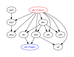
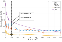
Parametric linear models have been popularly used for causal inference on this data-set [25, 11]. We fit a GLM gamma model [14] between the activation of each node and its parents in Fig. 3a using the observational data. In Section D.1 (in the appendix) we provide further details showing that the sampled distributions in the fitted model are extremely close to the empirical distributions from the data. The soft interventions signifying the arms are generated by changing the distribution of a source node pkc in the GLM. The objective is to identify the intervention that yields the highest output at the target node erk We provide empirical results for two sets of interventions at the source node. Both these experiments have been performed with $15$ arms each representing different distributions at pkc.

Budget Restriction: The experiments are performed in the budget setting S1, where all arms except arm $0$ are deemed to be difficult. We plot our results as a function of the total samples $T$, while the fractional budget of the difficult arms ($B$) is set to $1/\sqrt{T}$. Therefore, we have $\sum_{k\neq 0}T_{k}\leq\sqrt{T}$. This essentially belongs to the case when there is a lot of data that can be acquired for a default arm while any new change requires significant cost in acquiring samples.

Competing Algorithms: We test our algorithms on different problem parameters and compare with related prior work [3, 22]. The algorithms compared are (i) SRISv1: Algorithm 1 introduced in Section 2. The divergences, $D_{f_{1}}(P_{i}||P_{j})$ are estimated from sampled data using techniques from [30]; (ii)SRISv2: Algorithm 2 as detailed in Section 2; (iii) SR: Successive Rejects Algorithm from [3] adapted to the budget setting. The division of the total budget $T$ into $K-1$ phases is identical, while the individual arm budgets are decided in each phase according to the budget restrictions; (iv) CR: Algorithm 2 from [22]. The optimization problem for calculating the mixture parameter $\boldsymbol{\eta}$ is not efficiently solvable for general distributions and budget settings. Therefore, the mixture proportions are set by Algorithm 3.

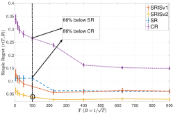
In these experiments, the budget restrictions imply that arm $0$ can be pulled much more than the other arms. Intuitively the divergences of the arms from arm $0$ as well as the gap $\Delta$ defines the hardness of identification. Fig. 3b represents a difficult scenario where the divergences $M_{k0}>400$ for many arms (large divergences imply low information leakage) and $\Delta=0.01$ (small $\Delta$ increases hardness). In Fig. 3c (easier scenario) the divergences $M_{k0}<20$ for most arms while the gap is same as before. We see that SRISv2 outperforms all the other algorithms by a large margin, especially in the low sample regime.

4.2 Interpretability of Inception Deep Network

In this section we use our algorithm for model interpretation of the pre-trained Inception-v3 network [38] for classifying images. Model Interpretation essentially addresses: ’why does a learning model classify in a certain way?’, which is an important question for complicated models like deep nets [31].

When an RGB image is fed to Inception, it produces an ordered sequence of $1000$ labels (e.g ’drums’, ’sunglasses’) and generally the top-$10$ labels are an accurate description of the objects in the image. To address interpretability, we segment the image into a number of superpixels/segments (using segmentation algorithms like SLIC [2]) and infer which superpixels encourage the neural net to output a certain label (henceforth referred to as label-I; e.g ’drum’) in top-$k$ (e.g. $k=10$), and to what extent.

(a)

(b)

(c)

(d)

Figure 4: Interpretation for different top labels for the image in (a); Image courtesy [9]. The best mixture distribution generates an image where the highlighted superpixels are most indicative of a label. For example, in (b) we see the drums highlighted, while in (d) (a different mixture distribution), sunglasses are in the focus.

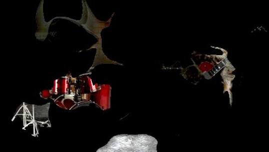
Given a mixture distribution over the superpixels of an image (Figure 4a), a few superpixels are randomly sampled from the distribution with replacement. Then a new image is generated where all other superpixels of the original image are blurred out except the ones selected. This image is then fed to Inception, and it is observed whether label-I appears within the top-$k$ labels. A mixture distribution is said to be a good interpretation for label-I if there is a high probability that label-I appears for an image generated by this mixture distribution. To empirically test the goodness of a mixture distribution, we would generate (using this mixture distribution) a number of random images, and determine the fraction of images for which label-I appears; a large fraction indicates that the mixture distribution is a good interpretation of label-I.

Motivated by the above discussion, we generate a large number ($3200$) of mixture distributions, with the goal of finding the one that best interprets label-I. To highlight the applicability of our algorithm, we allow images to be generated for only $200$ of these mixture distributions; in other words, most of the mixture distributions cannot be directly tested. Nevertheless, we determine the best from among the entire collection of mixture distributions (learning counterfactuals).

Specifically in our experiments, we consider the image in Figure 4a, partition it into $43$ superpixels, and generate images from mixture distributions by sampling $5$ superpixels (with replacement). We generate $3000$ arm distributions which lie in the $43$-dimensional simplex but have sparse support (sparsity of $10$ in our examples). The support of these distributions are randomly generated by techniques like markov random walk (encourages contiguity), random choice, etc. as detailed in Section D.2 in the appendix. However, we are only allowed to sample using a different set of $200$ arms that are dense distributions chosen uniformly at random from the $43$-dimensional simplex. The distributions are generated in a manner which is completely agnostic to the image content. The total sample budget ($T$) is $2500$.

Figure 4 shows images in which the segments are weighted in proportion to the optimal distribution (obtained by SRISv2) for the interpretation of three different labels. This showcases the true counterfactual power of the algorithm, as the set of arms that can be optimized over are disjoint from the arms that can be sampled from. Moreover the sample budget is less than the number of arms. This is an extreme special case of budget setting S2. We see that our algorithm can generate meaningful interpretations for all the labels with relatively less number of runs of Inception. Even sampling $10$ times from each of the arms to be optimized over would require $30,000$ runs of Inception for a single image and label, while we use only $2500$ runs by leveraging information leakage.

4.3 Synthetic Experiments

In this section, we empirically validate the performance our algorithm through synthetic experiments. We carefully design our simulation setting which is simple, but at the same time sufficient to capture the various tradeoffs involved in the problem. An important point to note is that our algorithm is not aware of the actual effect of the changes on the target (gaps between expectations) but it only knows the divergence among the candidate soft interventions. Sometimes, a change with large divergence from an existing one may not maximize the effect we are looking for. Conversely, smaller divergence may sometimes lead you closer to the optimal. We demonstrate that our algorithm performs well in all the experiments, as compared to previous works [3, 22].

Experimental Setup: We set up our experiments according to the simple causal graph in Figure 5. $V$ is assumed to be a random variable taking values in $\{0,1,2,\cdots,m-1\}$. The various arms $\mathrm{P}_{0}(V),\mathrm{P}_{1}(V),...\mathrm{P}_{K-1}(V)$ are discrete distributions with support $[m]$. We will vary $m$ and $K$ over the course of our experiments.

Figure 5: Causal Graph for Experimental Setup

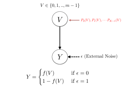
$Y$ is assumed to be a function of $V$ and some random noise $\epsilon$ which is external to the system. In our experiments, we set the function as follows:

$$Y=\begin{cases}f(V)&\text{ if }\epsilon=0\\ 1-f(V)&\text{ if }\epsilon=1\end{cases}$$

where $f:[m]\rightarrow\{0,1\}$ is an arbitrary function. We set ${\mathbb{P}}(\epsilon=1)=0.01$ in all our experiments. The discrete candidate distributions are modified to explore various tradeoffs between the gaps and the effective standard deviation parameters.

Budget Restriction: The experiments are performed in the budget setting S1, where all arms except arm $0$ are deemed to be difficult. We plot our results as a function of the total samples $T$, while the fractional budget of the difficult arms ($B$) is set to $1/\sqrt{T}$. Therefore, we have $\sum_{k\neq 0}T_{k}\leq\sqrt{T}$. This essentially belongs to the case when there is a lot of data that can be acquired for a default arm while any new change requires significant cost in acquiring samples.

Experiments: In our experiments, we choose $f$ to be the parity function, when $V\in[m]$, is represented in base $2$. Note that arm $0$ is the arm that can be sampled $O(T)$ times while the rest of the arms can only be sampled $O(\sqrt{T})$ times due to the above budget constraints. So, the divergence of the arm $0$ from other arms is crucial alongside the gaps. We perform our experiments in different regimes that get progressively easier. In these experiments, we function in various regimes of the divergences between the other arms and arm $0$, and the gaps from the optimal arm in terms of target value. When there is no information leakage, the samples are divided among the $K$ arms. So, the loss in having multiple arms can be expressed as a scaling $\sqrt{K}$ in standard deviation. Recall the $\log$ divergence measure $M_{k0}$ which is a measure of information leakage from arm $0$ to another arm $k$. Therefore, in the following, when we say high divergence from arm $0$, it means that $M_{k0}/\sqrt{K}$ is high for most arms $k\neq 0$.

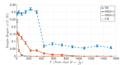
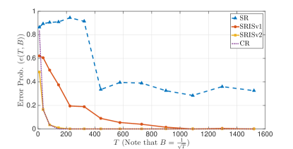
High Divergence and Low $\Delta$: This is the hardest of all settings. Here, we set $m=20$ and $K=30$. Here, we have $M_{k0}$ to be pretty high for all the arms $k\neq 0$. This means that the arm $0$, which can be pulled $O(T)$ times provides highly noisy estimates for other arms. We have $M_{k0}/\sqrt{K}\sim 30$ for most arms. Moreover, the minimum gap from the best arm $\Delta=0.04$, which is pretty small. This implies that it is harder to distinguish the best arm.

The results are demonstrated in Figure 6. Figure 6a displays the simple regret. We see that both SRISv1 and SRISv2 outperform the others by a large extent, in this hard setting, even when the number of samples are very low. In Figure 6b we plot the probability of error in exactly identifying the best arm. We see that none of the algorithms successfully identify the best arm, in the small sample regime, as the gap $\Delta$ is very low. However, our algorithms quickly zero in on arms that are almost as good as the optimal, and therefore the simple regret is well-behaved. Our algorithm performs this well even when the divergences are big, because it is able to reject the arms that have high $\Delta_{i}$ in the early phases, very effectively.

(a)

(b)

Figure 6: Performance of various algorithms when divergences $M_{k0}$’s are high and mininum gap $\Delta$ is small. The results are averaged over the course of $500$ independent experiments. The total sample budget $T$ is plotted on the $x$-axis. Note that budget for all arms other than arm $0$ is constrained to be less than $\sqrt{T}$. Here $K=30$.

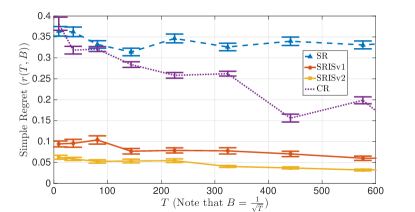
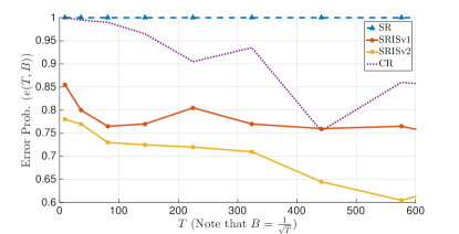
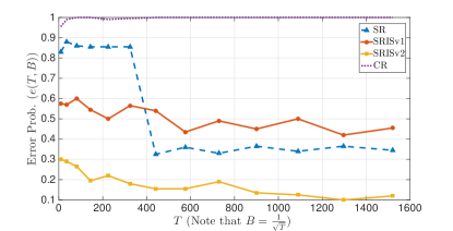
High Divergence and High $\Delta$: This is easier than the previous setting. Here, we set $m=10$ and $K=20$. Here, we have $M_{k0}$ to be very high for all the arms $k\neq 0$. Thus arm $0$ provides very noisy estimates on other arms. We have $M_{k0}/\sqrt{K}\gg 50$ for many arms. However, the minimum gap from the best arm $\Delta=0.15$, which is not too small. This implies that it might be easier to distinguish the best arm.

The results are demonstrated in Figure 7. Figure 7a displays the simple regret. We see that in the small sample regime SRISv1 and SRISv2 outperform the others by a large extent. In the high sample regime, SRISv2 is still the best, while SR and SRISv1 are close behind. In Figure 7b we plot the probability of error in exactly identifying the best arm. We see that SRISv2 performance very well in identifying the best arm even though arm $0$ gives highly noise estimates. It is interesting to note that CR does not perform well. This can be attributed to the non-adaptive clipper in CR, that incurs a significant bias because arm $0$ has high-divergences from most of the other arms.

(a)

(b)

Figure 7: Performance of various algorithms when divergences $M_{k0}$’s are high and min. gap $\Delta$ is not too bad. The results are averaged over the course of $500$ independent experiments. The total sample budget $T$ is plotted on the $x$-axis. Note that budget for all arms other than arm $0$ is constrained to be less than $\sqrt{T}$. Here, $K=20$.

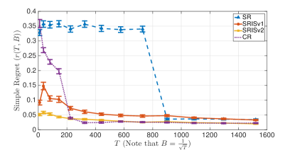
Low Divergence and Low $\Delta$: This is another moderately hard setting, similar to the previous one. Here, we set $m=20$ and $K=30$. Here, we have $M_{k0}$ to be not too high for the arms $k\neq 0$. This means that the arm $0$, which can be pulled $O(T)$ times is moderately good for estimating the other arms. Here, $M_{k0}/\sqrt{K}\leq 10$ for most arms $k$. However, the minimum gap from the best arm $\Delta=0.04$, which is small. This implies that it might be hard to distinguish the best arm.

The results are demonstrated in Figure 8. Figure 8a displays the simple regret. We see that in the small sample regime SRISv1 and SRISv2 outperforms the others by a large extent. In the high sample regime, SRISv2 is still the best, while CR is close behind. In Figure 8a we plot the probability of error in exactly identifying the best arm. We see that most of the algorithms have moderately bad probability of error as the gap $\Delta$ is small. However, the algorithms SRISv2 and SRISv1 are quickly able to zero down on arms close to optimal as shown in the simple regret in the small sample regime.

(a)

(b)

Figure 8: Performance of various algorithms when divergences $M_{k0}$’s are moderately low and min. gap $\Delta$ is small. The results are averaged over the course of $500$ independent experiments. The total sample budget $T$ is plotted on the $x$-axis. Note that budget for all arms other than arm $0$ is constrained to be less than $\sqrt{T}$. Here, $K=30$.

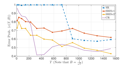
Low Divergence and High $\Delta$: This is the easiest of all settings. Here, we set $m=10$ and $K=20$. Here, arms $0$ has $\mathrm{P}_{0}(V)$ pretty close to the uniform distribution on $[m]$. Therefore, it is very well-posed for estimating the means of all other arms. In fact we have $M_{k0}/\sqrt{K}<2$ for many arms. Moreover, the minimum gap from the best arm $\Delta=0.15$, which is not too small. This implies that it might be very easy to distinguish the best arm.

The results are demonstrated in Figure 9. Figure 9a displays the simple regret. We see that SRISv2 and CR perform extremely well closely followed by SRISv1. In Figure 9b we plot the probability of error in exactly identifying the best arm. Again SRISv2 and CR have almost zero probability of error and SRISv1 is close behind. This is because $\Delta$ is pretty large. In this example, we observe that all the algorithms that use information leakage are better than SR, because arm $0$ is well-behaved. CR performs almost as well as SRISv2 in this example, as the static clipper is never invoked because almost always the ratios in the importance sampler are well bounded.

(a)

(b)

Figure 9: Performance of various algorithms when divergences $M_{k0}$’s are low and min. gap $\Delta$ is not too bad. The results are averaged over the course of $500$ independent experiments. The total sample budget $T$ is plotted on the $x$-axis. Note that budget for all arms other than arm $0$ is constrained to be less than $\sqrt{T}$. Here $K=20$.

In conclusion, it should be noted that our algorithms perform well in all the different settings, because they are able to adapt to the problem parameters (similar to  [3]) and at the same time leverage the information leakage (similar to  [22]).

5 Discussion and Future Work

In this paper, we analyze the problem of identifying the best arm at a node $V$ in a causal graph (various known conditionals $\mathrm{P}_{k}(V|pa(V)))$ in terms of its effect on a target variable $Y$ further downstream, possibly in a less understood portion of the larger causal network. We characterize the hardness of this problem in terms of the relative divergences of the various conditionals that are being tested and the gaps between the expected value of the target under the various arms. We provide the first problem dependent simple regret and error bounds for this problem, that is a natural generalization of  [3], but with information leakage between arms. We provide an efficient successive rejects style algorithm that achieves these guarantees, by leveraging the leakage of information, through carefully designed clipped importance samplers. Further, we introduce a new $f$-divergence measure that may be relevant for analyzing importance sampling estimators in the causal context. This may be of independent interest. We believe that our work paves the way for various interesting problems with significant practical implications. In the following, we state a few open questions in this regard:

Tighter guarantees on SRISv2: In Section 4, we have observed that a slightly modified version of our algorithm SRISv2 performs the best among all the competing algorithms including SRISv1. The only difference of SRISv2 from Algorithm 1, is that in line 6 the estimators used in a phase also uses samples from past phases, but clipped according to the criterion in the current phase. We believe that this algorithm has tighter error and simple regret guarantees. We conjecture that at least one of the $\log(1/\Delta_{k})$, in the definition of $\bar{H}$ in (6) can be eliminated, thus leading to better guarantees.

Estimating the marginals of the parents: In Algorithm 1, either the marginals of the parents of $V$, that is $\mathrm{P}(pa(V))$ is required in order to calculate the $f$-divergences in Definition 2, or prior data involving the parents is required to estimate the $f$-divergences directly from data. However, we believe it is possible to model this estimation, directly into the online framework, as data about the marginals of the parents are available through the samples in all the arms, as these marginals remain unchanged.

Problem Dependent Lower Bound: In [22], a problem independent lower bound of $O(1/\sqrt{T})$ has been provided for a special causal graph. However, the problem parameter dependent lower bound like that of [3] still remains an open problem. We believe that the lower bound will depend on the divergences between the distributions and the gaps between the rewards of the arms, similar to the term in (6).

General Learning Framework: Our work paves the way for a more general setting for learning counterfactual effects. Importance sampling is a fairly general tool and can be ideally applied at any set of nodes of a causal graph. So, in principle it is possible to study the effect of a change at $V$ on a target $Y$, by using importance sampling between the changed marginal distributions at an intermediate cut ${\cal S}$ that blocks every path from $V$ to $Y$. In fact, this is explored in a non-bandit context in [7]. An important question is: What is the most suitable cut to be used? [22] uses the cut closest to $Y$, i.e. immediate parents of $Y$. However, the marginals of the cut under different changes need to be estimated this ’far’ from the source closer to the target. Therefore, there is a tradeoff that involves a delicate balance between the estimation errors of the changes at an intermediate cut between $V$ and $Y$, and the reduction in importance sampling divergences between cut distributions closer to the target $Y$. We believe understanding this is quite important to fully exploit partial/full knowledge about causal graph structure to answer causal strength questions from data observed.

Appendix A Variations of the Problem Setting

In this section we provide more general causal settings where our results can be directly applied.

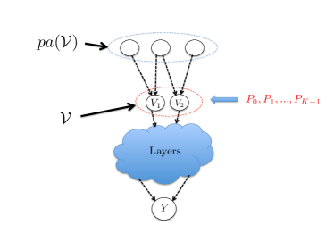
Multiple nodes at the graph: This is illustrated in Fig. 10a. Soft interventions can be performed at multiple nodes like at $\mathcal{V}=\{V_{1},V_{2}\}$. These interventions can be modeled as changing the distribution $P(\mathcal{V}|pa(\mathcal{V}))$ where $pa(\mathcal{V})$ are the union of parents of $V_{1}$ and $V_{2}$. These distributions can be thought of as the arms of the bandits and our techniques can be applied as before to estimate the best intervention.

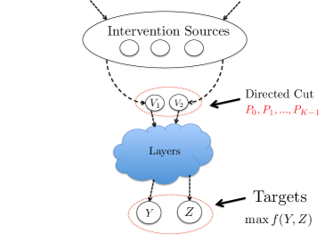
Directed cut between sources and targets: Fig. 10b represents the most general scenario in which our techniques can be applied. Soft or hard interventions can be performed at multiple source nodes, while the goal is to choose the best out of these interventions in terms of maximizing a known function of multiple target nodes. If the effect of these interventions can be estimated on a directed cut separating the targets and the sources then our techniques can be applied as before. This is akin to knowing $P(V_{1},V_{2})$ under all the interventions in Fig. 10b, because $V_{1}$ and $V_{2}$ is a directed cut separating the sources and the targets.

Empirical knowledge of continuous arm distributions: Our techniques can be applied to continuous distributions $\mathrm{P}(V|pa(V))$ as shown in our empirical results in Section 4.1. The extension is straight-forward by using the general definition of $f$-divergences. More importantly our techniques can be applied even if only prior empirical samples from the distributions $\mathrm{P}(V|pa(V))$ is available and not the whole distributions. In this case the $f$-divergences can be estimated using nearest neighbor estimators similar to [30]. Moreover, for the importance sampling only ratios of distributions are needed, which can again be estimated using nearest neighbor based techniques from empirical data.

(a)

(b)

Figure 10: Illustration of more general causal settings where our algorithms can be directly applied. (a) Illustration of a scenario where there are multiple intervention sources $\mathcal{V}=\{V_{1},V_{2}\}$. Each soft intervention is a change in the distribution $\mathrm{P}(\mathcal{V}|pa(\mathcal{V})).$ (b) Illustration of a causal setting, where there are many intervention sources. Soft or hard interventions can be performed at these sources and the effects of these interventions can be observed at the target node. Our techniques can be applied in choosing the best intervention in terms of maximizing a function on the target nodes, provided the effects of these interventions on $P(V_{1},V_{2})$ are known. Here $V_{1}$ and $V_{2}$ form a directed cut separating the sources and the targets

Appendix B Interpretation of our Theoretical Results

In this section we compare our theoretical bounds on the probability of mis-identification with the corresponding bounds in [3]. We also compare our simple regret guarantees with the guarantees in [22]. In both these cases, we demonstrate significant improvements. These theoretical improvements are exhibited in our empirical results in Section 4.1.

B.1 Comparison with [3]

Let $\tilde{{\cal R}}(\Delta_{k})=\{s:\Delta_{s}\leq\Delta_{k}\}$, i.e. the set of arms which are closer to the optimal than arm $k$. Let $\tilde{H}=\max\limits_{k\neq k*}\frac{\lvert\tilde{{\cal R}}(\Delta_{k})\rvert}{\Delta_{k}^{2}}$. The result for the best arm identification with no information leakage in [3] can be stated as: The error in finding the optimal arm is bounded as:

$$e(T)\leq O\left(K^{2}\exp\left(-\frac{T-K}{\overline{\log}(K)\tilde{H}}\right)\right)$$ (8)

One intuitive interpretation for $\tilde{H}$ is that it is the maximum among the number of samples (neglecting some log factors) required to conclude that arm $k$ is suboptimal from among the arms which are closer to the optimal than itself. Intuitively, this is because when there is no information leakage, one requires $1/\Delta_{k}^{2}$ samples to distinguish between the $k$-th optimal arm and the optimal arm. Further, the $k$th arm is played only $1/k$ fraction of the times since we do not know the identity of the $k$-th optimal arm.

Our main result in Theorem 1 can be seen to be a generalization of the existing result for the case when there is information leakage between the arms (various changes in a causal graph).

The term $\sigma^{*}(B,{\cal R}^{*}(\Delta_{k}))$ in our setting is the ‘effective standard deviation’ due to information leakage. There is a similar interpretation of our result (ignoring the log factors): Since there is information leakage, the expression $\frac{(\sigma^{*})^{2}}{(\Delta_{k})^{2}}$ characterizes the number of samples required to weed out arm $k$ out of contention from among competing arms (arms that are at a distance at most twice than that of arm $k$ from the optimal arm). The interpretation of ’effective variance’ is justified using importance sampling which is detailed in Section C.3. Further, in our framework $\sigma^{*}$ also incorporates any budget constraint that comes with the problem, i.e. any apriori constraint on the relative fraction of times different arms need to be pulled.

For ease of exposition let $(k)$ denote the index of the $k$-th best arm (for $k=1,..,K$) and $\Delta_{(k)}$ denotes the corresponding gap. In this setting, the terms $\tilde{H}$ (from the result in [3]) and $\bar{H}$ can be written as:

$$\tilde{H} =\max_{k\neq 1}\frac{k}{\Delta_{(k)}^{2}}$$

$$\bar{H} =\max_{k\neq 1}\frac{\sigma^{*}(B,{\cal R}^{*}(\Delta_{(k)}))^{2}}{\Delta_{(k)}^{2}}.$$

$\sigma^{*}(B,{\cal R}^{*}(\Delta_{(k)}))$ can be smaller than $\sqrt{k}$ due to information leakage as every single arm pull contributes to another arm’s estimate. Therefore, these provide better guarantees than  [3].

To see the improvement over the previous result in [3], we consider a special case when the cost budget $B$ is infinity and there is only the the sample budget $T$. In addition, let us assume that the log divergences are such that: $M_{ij}\leq\eta M_{ii}=\eta<<\sqrt{\lvert{\cal R}\rvert},~{}\forall i\neq j$. Let ${\cal R}={\cal R}^{*}(\Delta_{(k)})$. If $\eta>\sqrt{\lvert{\cal R}\rvert}$, the optimal solution for (4) is a bit complicated to interpret. Consider the feasible allocation $\nu_{i}=\frac{1}{\lvert{\cal R}\rvert},~{}\forall i\in{\cal R}$ in (4). Evaluating the objective function for this feasible allocation, it is possible to show that $\sigma^{*}\leq\frac{\eta}{1-1/\lvert{\cal R}\rvert}<<\sqrt{\lvert{\cal R}\rvert}$. Hence, unless the variance due to information leakage is too bad, the effective variance is smaller than that of the case with no information leakage.

The improvement over the no information leakage setting, is even more pronounced under budget constraints. Consider the setting S1, and assume that the fractional budget of the difficult arms, $B=o(1)$. This implies that the total number of samples available for difficult arms is $o(T)$. The budget constrained case has not been analyzed in [3], however in the absence of information leakage, one would expect that the arms with the least number of samples would be the most difficult to eliminate, and therefore the error guarantees would scale as $\exp(-O(BT)/\tilde{H})\sim\exp(-o(T)/\tilde{H})$ (excluding $\log$ factors). On the other hand, our algorithm can leverage the information leakage and the error guarantee would scale as $\exp(-O(T)/\bar{H})$, which can be order-wise better if the effective standard deviations are well-behaved.

B.2 Comparison with [22]

In [22], the algorithm is based on clipped importance samples, where the clipper is always set at a static level of $O(\sqrt{T})$ (excluding $\log$ factors). The simple regret guarantee in [22] scales as $O(\sqrt{(m(\eta)/T)\log T})$, where $m(\eta)$ is a global hardness parameter. The guarantees do not adapt to the problem parameters, specifically the gaps $\{\Delta_{k}\}_{k\in[K]}$.

On the contrary, we provide problem dependent bounds, which differentiates the arms according to its gap from the optimal arm and its effective standard deviation parameter. The terms $\bar{H}_{k}$ can be interpreted as the hardness parameter for rejecting arm $k$. Note that $\bar{H}_{k}$ depends only on the arms that are at least as bad in terms of their gap from the optimal arm. Moreover the guarantees are adapted to our general budget constraints, which is absent in [22]. It can be seen that when $\Delta_{k}$’s do not scale in $T$, then our simple regret is exponentially small in $T$ (dependent on $\bar{H}_{k}$’s) and can be much less than $O(1/\sqrt{T})$. The guarantee also generalizes to the problem independent setting when $\Delta_{k}$’s scale as $O(1/\sqrt{T})$.

Appendix C Proofs

In this section we present the theoretical analysis of our algorithm. Before we proceed to the proof of our main theorems, we derive some key lemmas that are useful in analyzing clipped importance sampled estimators.

C.1 Clipped Importance Sampling Estimator

In Section 3.1 we have introduced the concept of importance sampling that helps us in using samples collected under one arm to estimate the means of other arms. As noted in Section 3.1, a naive unbiased importance sampled estimator can potentially have unbounded variances thus leading to poor guarantees. We now introduce clipped importance samplers and provide a novel analysis of these estimators that alleviates the variance related issues.

Clipped Importance Samplers: The naive estimator of (2) is not suitable for yielding good confidence intervals. It has been observed in the context of importance sampling, that clipping the estimator in (2) at a carefully chosen value, can yield better confidence guarantees even though the resulting estimator will become slightly biased [7]. Before we introduce the precise estimator, let us define a key quantity that will be useful for the analysis.

Definition 4.

We define $\eta_{i,j}(\epsilon)$ as follows:

$$\eta_{i,j}(\epsilon)=\left\{\operatorname*{\arg\!\min}_{\eta}:{\mathbb{P}}_{i}\left(\frac{\mathrm{P}_{i}(V|pa(V))}{\mathrm{P}_{j}(V|pa(V))}>\eta\right)\leq\frac{\epsilon}{2}\right\}$$ (9)

for all $i,j\in[K]$, where $\epsilon>0$.

We shall see that the $\eta_{i,j}(\epsilon)$ is related to the conditional $f$-divergence between $\mathrm{P}_{i}(V|pa(V))$ and $\mathrm{P}_{j}(V|pa(V))$ for the carefully chosen function $f_{1}(.)$ as introduced in Section 3.1.

Now we are at a position to provide confidence guarantees on the following clipped estimator:

$$\hat{Y}^{(\eta)}_{i}(j)=\frac{1}{t}\sum_{s=1}^{t}Y_{j}(s)\frac{\mathrm{P}_{i}(V_{j}(s)|pa(V)_{j}(s))}{\mathrm{P}_{j}(V_{j}(s)|pa(V)_{j}(s))}\times\mathds{1}\left\{\frac{\mathrm{P}_{i}(V_{j}(s)|pa(V)_{j}(s))}{\mathrm{P}_{j}(V_{j}(s)|pa(V)_{j}(s))}\leq\eta_{ij}(\epsilon)\right\}.$$ (10)

Lemma 1.

The estimate $\hat{Y}^{(\eta)}_{i}(j)$ for $\eta=\eta_{i,j}(\epsilon)$ satisfies the following:

1. $${\mathbb{E}}_{j}\left[\hat{Y}^{(\eta)}_{i}(j)\right]\leq\mu_{i}\leq{\mathbb{E}}_{j}\left[\hat{Y}^{(\eta)}_{i}(j)\right]+\frac{\epsilon}{2}$$ (11)

2. $${\mathbb{P}}\left(\mu_{i}-\delta-\epsilon/2\leq\hat{Y}^{(\eta)}_{i}(j)\leq\mu_{i}+\delta\right)\geq 1-2\exp\left(-\frac{\delta^{2}t}{2\eta_{i,j}(\epsilon)^{2}}\right).$$ (12)

Proof.

We have the following chain:

$${\mathbb{E}}_{j}\left[Y\frac{\mathrm{P}_{i}(V|pa(V)}{\mathrm{P}_{j}(V|pa(V))}\right]$$

$$={\mathbb{E}}_{j}\left[Y\frac{\mathrm{P}_{i}(V|pa(V))}{\mathrm{P}_{j}(V|pa(V))}\mathds{1}\left\{\frac{\mathrm{P}_{i}(V|pa(V))}{\mathrm{P}_{j}(V|pa(V))}\leq\eta_{i,j}(\epsilon)\right\}\right]+{\mathbb{E}}_{j}\left[Y\frac{\mathrm{P}_{i}(V|pa(V))}{\mathrm{P}_{j}(V|pa(V))}\mathds{1}\left\{\frac{\mathrm{P}_{i}(V|pa(V))}{\mathrm{P}_{j}(V|pa(V))}>\eta_{i,j}(\epsilon)\right\}\right]$$

$$\overset{(a)}{\leq}{\mathbb{E}}_{j}\left[Y\frac{\mathrm{P}_{i}(V|pa(V))}{\mathrm{P}_{j}(V|pa(V))}\mathds{1}\left\{\frac{\mathrm{P}_{i}(V|pa(V))}{\mathrm{P}_{j}(V|pa(V))}\leq\eta_{i,j}(\epsilon)\right\}\right]+{\mathbb{P}}_{i}\left(\frac{\mathrm{P}_{i}(V|pa(V))}{\mathrm{P}_{j}(V|pa(V))}>\eta_{i,j}(\epsilon)\right)$$

$$\leq{\mathbb{E}}_{j}\left[Y\frac{\mathrm{P}_{i}(V|pa(V))}{\mathrm{P}_{j}(V|pa(V))}\mathds{1}\left\{\frac{\mathrm{P}_{i}(V|pa(V))}{\mathrm{P}_{j}(V|pa(V))}\leq\eta_{i,j}(\epsilon)\right\}\right]+\frac{\epsilon}{2}$$

Here, $(a)$ is because $Y\in[0,1]$. This yields the first part of the lemma:

$${\mathbb{E}}_{j}\left[\hat{Y}^{(\eta)}_{i}(j)\right]\leq\mu_{i}\leq{\mathbb{E}}_{j}\left[\hat{Y}^{(\eta)}_{i}(j)\right]+\frac{\epsilon}{2}$$ (13)

where $\eta=\eta_{i,j}(\epsilon)$. Note that all the terms in the summation of (10) are bounded by $\eta_{i,j}(\epsilon)$. Therefore, by an application of Azuma-Hoeffding we obtain:

$${\mathbb{P}}\left(\lvert\hat{Y}^{(\eta)}_{i}(j)-{\mathbb{E}}_{j}\left[\hat{Y}^{(\eta)}_{i}(j)\right]\rvert>\delta\right)\leq 2\exp\left(-\frac{\delta^{2}t}{2\eta_{i,j}(\epsilon)^{2}}\right)$$ (14)

Combining Equation (13) and (14), we obtain the first part of our lemma. ∎

C.2 Relating $\eta_{ij}(\cdot)$ with $f$-divergence

Now we are left with relating $\eta_{i,j}(\epsilon)$ to a particular $f$-divergence ($D_{f_{1}}$ defined in Section 3.1) between $\mathrm{P}_{i}(V|pa(V))$ and $\mathrm{P}_{j}(V|pa(V))$. We have the following relation,

$$\mathbb{E}_{i}\left[\exp\left(\frac{\mathrm{P}_{i}(V|pa(V))}{\mathrm{P}_{j}(V|pa(V))}\right)\right]=\left[1+D_{f_{1}}\left(\mathrm{P}_{i}\lVert\mathrm{P}_{j}\right)\right]e.$$ (15)

The following lemma expresses the quantity $\eta_{i,j}(\epsilon)$ as a separable function of $D_{f_{1}}\left(\mathrm{P}_{i}\lVert\mathrm{P}_{j}\right)$ and $\epsilon$, and is one of the key tools used in subsequent analysis.

Lemma 2.

It holds that, $\eta_{i,j}(\epsilon)\leq\log\left(\frac{2}{\epsilon}\right)+1+\log\left(1+D_{f_{1}}\left(\mathrm{P}_{i}\lVert\mathrm{P}_{j}\right)\right)$. Furthermore,

$$\eta_{i,j}(\epsilon)\leq 2\log\left(\frac{2}{\epsilon}\right)\left[1+\log(1+D_{f_{1}}(\mathrm{P}_{i}\lVert\mathrm{P}_{j}))\right]$$ (16)

when, $\epsilon\leq 1$.

Proof.

We have the following chain:

$$\mathbb{P}_{i}\left(\frac{\mathrm{P}_{i}(V|pa(V))}{\mathrm{P}_{j}(V|pa(V))}>\eta\right)$$ (17)

$$=\mathbb{P}_{i}\left(\exp\left(\frac{\mathrm{P}_{i}(V|pa(V))}{\mathrm{P}_{j}(V|pa(V))}\right)>\exp(\eta)\right)$$

$$\overset{(a)}{\leq}\mathbb{E}_{i}\left[\exp\left(\frac{\mathrm{P}_{i}(V|pa(V))}{\mathrm{P}_{j}(V|pa(V))}\right)\right]\exp(-\eta)$$

(a) - We used Markov’s inequality. Suppose, we have the right hand side to be at most $\epsilon/2$. Then we have,

$$\mathbb{E}_{i}\left[\exp\left(\frac{\mathrm{P}_{i}(V|pa(V))}{\mathrm{P}_{j}(V|pa(V))}\right)\right]\exp(-\eta)\leq\epsilon/2$$ (19)

Now using (15), we have:

$$\eta\geq\log\left(\frac{2}{\epsilon}\right)+1+\log(1+D_{f_{1}}(\mathrm{P}_{i}\lVert\mathrm{P}_{j}))$$ (20)

$$\implies\mathbb{P}_{i}\left(\frac{\mathrm{P}_{i}(V|pa(V))}{\mathrm{P}_{j}(V|pa(V))}>\eta\right)\leq\epsilon/2$$

From, the definition of $\eta_{i,j}(\epsilon)$, we have:

$$\eta_{i,j}(\epsilon) \leq\log\left(\frac{2}{\epsilon}\right)+1+\log(1+D_{f_{1}}(\mathrm{P}_{i}\lVert\mathrm{P}_{j}))$$

$$\overset{a}{\leq}2\log\left(\frac{2}{\epsilon}\right)\left[1+\log(1+D_{f_{1}}(\mathrm{P}_{i}\lVert\mathrm{P}_{j}))\right],~{}\forall\epsilon\leq 1$$ (21)

(a) - This is due to the inequality $p+q\leq 2pq$ when $q\geq 1$ and $p\geq\log_{e}(2)$. ∎

Now, we introduce the main result of this section as Theorem 3. Recall that $M_{ij}=1+\log(1+D_{f_{1}}(\mathrm{P}_{i}\lVert\mathrm{P}_{j}))$.

Theorem 3.

The estimate $\hat{Y}^{(\eta)}_{i}(j)$ for $\eta=2\log(2/\epsilon)M_{ij}$ satisfies the following confidence guarantees:

$${\mathbb{P}}\left(\mu_{i}-\delta-\epsilon/2\leq\hat{Y}^{(\eta)}_{i}(j)\leq\mu_{i}+\delta\right)\geq 1-2\exp\left(-\frac{\delta^{2}t}{8\log(2/\epsilon)^{2}M_{ij}^{2}}\right).$$

Proof.

The proof is immediate from Lemmas 2 and 1. ∎

C.3 Aggregating Heterogenous Clipped Estimators

In Section C.1, we have seen how samples from one of the candidate distribution can be used for estimating the target mean under another arm. Therefore, it is possible to obtain information about the target mean under the $k^{th}$ arm (${\mathbb{E}}_{k}[Y]$) from the samples of all the other arms. It is imperative to design an efficient estimator of ${\mathbb{E}}_{k}[Y]$ ($\forall k\in[K]$) that seamlessly uses the samples from all arms, possibly with variable weights depending on the relative divergences between the distributions. In this section we will come up with one such estimator, based on the insight gained in Section C.1.

Recall the quantities $M_{kj}=1+\log(1+D_{f_{1}}(\mathrm{P}_{k}\lVert\mathrm{P}_{j}))$ ($\forall k,j\in[K]$). These quantities will be the key tools in designing the estimators in this section. Suppose we obtain $\tau_{i}$ samples from arm $i\in[K]$. Let the total number of samples from all arms put together be $\tau$.

Let us index all the samples by $s\in\{1,2,..,\tau\}$. Let $\mathcal{T}_{k}\subset\{1,2,..,\tau\}$ be the indices of all the samples collected from arm $k$. Further, let $Z_{k}=\sum_{j\in[K]}\tau_{j}/M_{kj}$. Now, we are at the position to introduce the estimator for $\mu_{k}$, which we will denoted by $\hat{Y}_{k}^{\epsilon}$ ($\epsilon$ is an indicator of the level of confidence desired):

$$\hat{Y}_{k}^{\epsilon}=\frac{1}{Z_{k}}\sum_{j=0}^{K}\sum_{s\in\mathcal{T}_{j}}\frac{1}{M_{kj}}Y_{j}(s)\frac{\mathrm{P}_{k}(V_{j}(s)|pa(V)_{j}(s))}{\mathrm{P}_{j}(V_{j}(s)|pa(V)_{j}(s))}\times\mathds{1}\left\{\frac{\mathrm{P}_{k}(V_{j}(s)|pa(V)_{j}(s))}{\mathrm{P}_{j}(V_{j}(s)|pa(V)_{j}(s))}\leq 2\log(2/\epsilon)M_{kj}\right\}.$$ (22)

In other words, $\hat{Y}_{k}^{\epsilon}$ is the weighted average of the clipped samples, where the samples from arm $j$ are weighted by $1/M_{kj}$ and clipped at $2\log(2/\epsilon)M_{kj}$.

Lemma 3.

$$\hat{\mu}_{k}:={\mathbb{E}}\left[\hat{Y}^{\epsilon}_{k}\right]\leq\mu_{k}\leq{\mathbb{E}}\left[\hat{Y}^{\epsilon}_{k}\right]+\frac{\epsilon}{2}$$ (23)

Proof.

We note that $\hat{Y}_{k}^{\epsilon}$ can be written as:

$$\hat{Y}_{k}^{\epsilon}=\frac{1}{Z_{k}}\sum_{j=0}^{K}\frac{\tau_{j}}{M_{kj}}\tilde{Y}_{kj}^{\epsilon}$$ (24)

Here, $\tilde{Y}_{kj}^{\epsilon}=\frac{1}{\tau_{j}}\sum_{s\in\mathcal{T}_{j}}Y_{j}(s)\frac{\mathrm{P}_{k}(V_{j}(s)|pa(V)_{j}(s))}{\mathrm{P}_{j}(V_{j}(s)|pa(V)_{j}(s))}$ $\times\mathds{1}\left\{\frac{\mathrm{P}_{k}(V_{j}(s)|pa(V)_{j}(s))}{\mathrm{P}_{j}(V_{j}(s)|pa(V)_{j}(s))}\leq 2\log(2/\epsilon)M_{kj}\right\}$. Using Lemma 2 it is easy to observe that $\mathbb{E}[\tilde{Y}_{k}^{\epsilon}]\leq\mu_{k}\leq\mathbb{E}[\tilde{Y}_{k}^{\epsilon}]+\frac{\epsilon}{2}$ as $\eta_{kj}(\epsilon)\leq 2\log(2/\epsilon)M_{kj}$. Now, (24) together with this implies the lemma as $Z_{k}=\sum_{j\in[K]}\tau_{j}/M_{kj}$.

∎

Theorem 4.

The estimator $\hat{Y}_{k}^{\epsilon}$ of (22) satisfies the following concentration guarantee:

$${\mathbb{P}}\left(\mu_{k}-\delta-\epsilon/2\leq\hat{Y}^{\epsilon}_{k}\leq\mu_{k}+\delta\right)\geq 1-2\exp\left(-\frac{\delta^{2}\tau}{8(\log(2/\epsilon))^{2}}\left(\frac{Z_{k}}{\tau}\right)^{2}\right)$$

Proof.

For the sake of analysis, let us consider the rescaled version $\bar{Y}_{k}^{\epsilon}=(Z_{k}/\tau)\hat{Y}_{k}^{\epsilon}$ which can be written as:

$$\bar{Y}_{k}^{\epsilon}=\frac{1}{\tau}\sum_{j=0}^{K}\sum_{s\in\mathcal{T}_{j}}\frac{1}{M_{kj}}Y_{j}(s)\frac{\mathrm{P}_{k}(V_{j}(s)|pa(V)_{j}(s))}{\mathrm{P}_{j}(V_{j}(s)|pa(V)_{j}(s))}\times\mathds{1}\left\{\frac{\mathrm{P}_{k}(V_{j}(s)|pa(V)_{j}(s))}{\mathrm{P}_{j}(V_{j}(s)|pa(V)_{j}(s))}\leq 2\log(2/\epsilon)M_{kj}\right\}.$$ (25)

Since $Y_{j}(s)\leq 1$, we have every random variable in the sum in (25) bounded by $2\log(2/\epsilon)$

Let, $\bar{\mu}_{k}=\mathbb{E}[\bar{Y}_{k}^{\epsilon}]$. Therefore by Chernoff’s bound, we have the following chain:

$${\mathbb{P}}\left(\lvert\bar{Y}_{k}-\bar{\mu}_{k}\rvert\leq\delta\right)\leq 2\exp\left(-\frac{\delta^{2}\tau}{8(\log(2/\epsilon))^{2}}\right)$$

$$\implies{\mathbb{P}}\left(\lvert\bar{Y}_{k}\frac{\tau}{Z_{k}}-\bar{\mu}_{k}\frac{\tau}{Z_{k}}\rvert\leq\delta\frac{\tau}{Z_{k}}\right)\leq 2\exp\left(-\frac{\delta^{2}\tau}{8(\log(2/\epsilon))^{2}}\right)$$

$$\implies{\mathbb{P}}\left(\lvert\hat{Y}_{k}-\hat{\mu}_{k}\rvert\leq\delta\frac{\tau}{Z_{k}}\right)\leq 2\exp\left(-\frac{\delta^{2}\tau}{8(\log(2/\epsilon))^{2}}\right)$$

$$\implies{\mathbb{P}}\left(\lvert\hat{Y}_{k}-\hat{\mu}_{k}\rvert\leq\delta\right)\leq 2\exp\left(-\frac{\delta^{2}\tau}{8(\log(2/\epsilon))^{2}}\left(\frac{Z_{k}}{\tau}\right)^{2}\right)$$ (26)

Now we can combine Equations (C.3) and (23) we get:

$${\mathbb{P}}\left(\mu_{k}-\delta-\epsilon/2\leq\hat{Y}^{\epsilon}_{k}\leq\mu_{k}+\delta\right)\geq 1-2\exp\left(-\frac{\delta^{2}\tau}{8(\log(2/\epsilon))^{2}}\left(\frac{Z_{k}}{\tau}\right)^{2}\right)$$

∎

In Theorem 4, we observe that the first part of the exponent scales as $O(\epsilon^{2}\tau/(\log(2/\epsilon))^{2})$ if we set $\delta=O(\epsilon)$, which is very close to the usual Chernoff’s bound with $\tau$ i.i.d samples. The performance of this estimator therefore depends on the factor $(Z_{k}/\tau)$ which depends on the fixed quantities $M_{kj}$ ($\forall j$) and the allocation of the samples $\tau_{j}$. In the next section, we will come up with a strategy to allocate the samples so that the estimators $\hat{Y}_{k}^{\epsilon}$ have good guarantees for all the arms $k$.

C.4 Allocation of Samples

In Section C.3, Theorem 4 tells us that the confidence guarantees on the estimator depends on how the samples are allocated between the arms. To be more precise, the term $(Z_{k}/\tau)$ in Equation (C.3), affects the performance of the estimator for $\mu_{k}$ ($\hat{Y}_{k}^{\epsilon}$). We would like to maximize $(Z_{k}/\tau)$ for all arms $k\in[K]$.

Let the total budget be $\tau$. Let ${\cal R}$ be the set of arms that remain in contention for the best optimal arm. Consider the matrix $\mathbf{A}\in\mathbb{R}^{K\times K}$ such that $\mathbf{A}_{kj}=1/M_{kj}$ for all $k,j\in[K]$. Then, we decide the fraction of times arm $k$ gets pulled, i.e. $\nu_{k}$ to maximize $Z_{k}$ using the Algorithm 3.

Lemma 4.

Allocation $\boldsymbol{\tau}$ in Algorithm 3 ensures that $(Z_{k}/\tau)\geq\frac{1}{\sigma^{*}(B,{\cal R})}$ for all $k\in{\cal R}$.

This is essentially the best allocation of the individual arm budgets in terms of ensuring good error bounds on the estimators $\hat{Y}_{k}^{\epsilon}$ for all $k\in\mathcal{R}$. Since S1 is a special case of S2, to obtain the allocation for S1 one needs to set the cost values $c_{i}$ set to $1$ for $i\in{\cal B}$ (difficult arms) in the above formulation and $0$ otherwise.

C.5 Putting it together: Online Analysis

We analyze Algorithm 1 phase by phase. With some abuse of notation, we redefine various quantities to be used in the analysis of the algorithm. Each quantity depends on the phase indices, as follows:

• $\mathcal{R}(l)$: Set of arms remaining after phase $l-1$ ends.

• $\hat{Y}_{k}(l)$: The value of the estimator (in Algorithm 1) for arm $k$ at the end of phase $l$.

• $\hat{Y}_{H}(l)$: The value of the highest estimate $\max_{k}\hat{Y}_{k}(l)$ (in Algorithm 1).

• $\mathcal{A}(l)\subseteq\mathcal{R}(l)$: Set of arms given by:

  $$\mathcal{A}(l):=\left\{k\in\mathcal{R}(l):\Delta_{k}>\frac{10}{2^{l}}\right\}.$$ (27)

• $S_{l}$: Success event of phase $l$ defined as:

  $$S_{l}:= \cap_{k\in\mathcal{R}(l),k\neq k^{*}}\left\{\hat{Y}_{k}(l)\leq\mu_{k}+\frac{1}{2^{l-1}}\right\}\cap\left\{\mu_{k}-\frac{3}{2^{l}}\leq\hat{Y}_{k^{*}}(l)\right\}.$$ (28)

Now we will establish that the occurrence of the event $S_{l}$ implies that all arms in $\mathcal{A}(l)$ gets eliminated at the end of phase $l$, while at the same time the optimal arm survives. Consider an arm $k\in\mathcal{A}(l)$. Given $S_{l}$ has happened we have:

$$\hat{Y}_{H}(l) \geq\hat{Y}_{k^{*}}(l)\geq\mu_{k^{*}}-\frac{3}{2^{l}}$$

$$\hat{Y}_{k}(l) \leq\mu_{k}+\frac{1}{2^{l-1}}$$

This further implies that $\hat{Y}_{H}(l)-\hat{Y}_{k}(l)\geq\Delta_{k}-5/2^{l}>5/2^{l}$. Therefore all the arms in $\mathcal{A}(l)$ are eliminated given $S_{l}$. Following similar logic it is also possible to show that the optimal arm survives. If $\hat{Y}_{H}(l)=Y_{k*}(l)$ then it survives certainly. Now, given $S_{l}$, only arms in $\mathcal{R}(l)\setminus\mathcal{A}(l)$ can be the ones with the highest means. Consider arms $k\in\mathcal{R}(l)\setminus\mathcal{A}(l)$. Again given $S_{l}$ we have:

$$\hat{Y}_{k^{*}}(l) \geq\mu_{k^{*}}-\frac{3}{2^{l}}$$

$$\hat{Y}_{k}(l) \leq\mu_{k}+\frac{1}{2^{l-1}}$$

Therefore, we have $Y_{k}(l)-Y_{k^{*}}(l)\leq 5/2^{l}-\Delta_{k}<5/2^{l}$. Therefore, the optimal arm survives.

It would seem that now it would be easy to analyze the probability of the event $S_{l}$, using Theorem 4. However, the bound in Theorem 4 depends on the sequence of arms eliminated so far in each phase. Therefore it is imperative to analyze $S_{1:l}$, that is the event that all phases from $1,2,..,l$ succeed. Let $B_{l}={\mathbb{P}}(S_{l}^{c}|S_{1:l-1})$. So, we have the chain:

$${\mathbb{P}}(S_{1:l}) \geq{\mathbb{P}}(S_{1:l}|S_{1:l-1}){\mathbb{P}}(S_{1:l-1})$$

$$\geq{\mathbb{P}}(S_{1:l}|S_{1:l-1}){\mathbb{P}}(S_{1:l-1}|S_{1:l-2}){\mathbb{P}}(S_{1:l-2})$$

$$\geq\prod_{i=0}^{l-2}{\mathbb{P}}(S_{1:l-i}|S_{1:l-i-1})P(S_{1})$$

$$=\prod_{s=1}^{l}(1-B_{s})$$

$$\geq 1-\sum_{s=1}^{l}B_{s}$$

The advantage of analyzing the probability of $S_{1:l}$ is that given $S_{1:l}$ we know the exact sequences of the arms that have been eliminated till Phase $l$. This gives us exact control on the exponents in the bound of Theorem 4. Given $S_{1:s-1}$ we have,

$$\mathcal{R}(s)\subseteq\mathcal{R}^{*}(s):=\left\{k:\Delta_{k}\leq\frac{10}{2^{s-1}}\right\}.$$

Recall that the budget for the samples of each arm in any phase $s$, is decide by solving the LP in Algorithm 3. Therefore, given $S_{1:s-1}$, we have $\sigma^{*}(B,{\cal R}(s))\geq\sigma^{*}(B,{\cal R}^{*}(s))$. Therefore, we have the following key lemma.

Lemma 5.

We have:

$$B_{l} :={\mathbb{P}}\left(S_{l}^{c}|S_{1:l-1}\right)\leq 2\lvert\mathcal{R}^{*}(l)\rvert\exp\left(-\frac{2^{-2(l-1)}\tau(l)v^{*}(B,{\cal R}^{*}(l))^{2}}{8l^{2}}\right)$$ (29)

Proof.

Note that in this phase we set $\eta_{kj}=2lM_{kj}$. Setting $\epsilon=2^{-(l-1)}$ and $\delta=2^{-(l-1)}$ in Theorem 4 and by Lemma 4 we have:

$${\mathbb{P}}\left(\mu_{k}-\frac{3}{2^{l}}\leq\hat{Y}_{k}(l)\leq\mu_{k}+\frac{1}{2^{l-1}}\right)\geq 1-2\exp\left(-\frac{2^{-2(l-1)}\tau(l)v^{*}(B,{\cal R}^{*}(l))^{2}}{8l^{2}}\right)$$ (30)

Note that the samples considered in phase $l$ are independent of the event $S_{1:l-1}$. Doing a union bound of the event complementary to the success event in (28), for all the remaining arms in $\mathcal{R}^{*}(\ell)$ implies the result in the Lemma. ∎

Now we are at a position to introduce our main results as Theorem 5.

Theorem 5.

Consider a problem instance with $K$ candidate arms $\{\mathrm{P}_{k}(V|pa(V)\}_{k=0}^{K-1}$. Let the gaps from the optimal arm be $\Delta_{k}$ for $k\in[K]$. Let us define the following important quantities:

$${\cal R}^{*}(\Delta_{k})=\left\{s:\Bigg{\lfloor}\log_{2}\left(\frac{10}{\Delta_{s}}\right)\Bigg{\rfloor}\geq\Bigg{\lfloor}\log_{2}\left(\frac{10}{\Delta_{k}}\right)\Bigg{\rfloor}\right\}$$ (31)

$$\bar{H}_{k}=\max_{\{l:\Delta_{l}\geq\Delta_{k}\}}\frac{\log_{2}(10/\Delta_{l})^{3}}{(\Delta_{l}/10)^{2}v^{*}(B,{\cal R}^{*}(\Delta_{l}))^{2}}$$ (32)

$$\bar{H}=\max_{k\neq k^{*}}\frac{\log_{2}(10/\Delta_{k})^{3}}{(\Delta_{k}/10)^{2}v^{*}(B,{\cal R}^{*}(\Delta_{k}))^{2}}$$ (33)

Algorithm 1 satisfies the following guarantees:

1. The simple regret is bounded as:

$$r(T,B)\leq 2K^{2}\sum_{\begin{subarray}{c}k\neq k^{*}:\\ \Delta_{k}\geq 10/\sqrt{T}\end{subarray}}\Delta_{k}\log_{2}\left(\frac{20}{\Delta_{k}}\right)\exp\left(-\frac{T}{2\bar{H}_{k}\overline{\log}(n(T))}\right)$$

$$+\frac{10}{\sqrt{T}}\mathds{1}\left\{\exists k\neq k^{*}\text{ s.t }\Delta_{k}<10/\sqrt{T}\right\}$$

2. The error probability is bounded as:

$$e(T,B)\leq 2K^{2}\log_{2}(20/\Delta)\exp\left(-\frac{T}{2\bar{H}\overline{\log}(n(T))}\right)$$

The bound on the error probability only holds if $\Delta_{k}\geq 10/\sqrt{T}$ for all $k\neq k^{*}$.

Proof.

Recall that the simple regret is given by:

$$r(T,B)=\sum_{k\neq k^{*}}\Delta_{k}{\mathbb{P}}\left(\hat{k}(T,B)=k\right)$$ (34)

Let us introduce some further notation. Let us define the phase at which an arm is ideally deleted as follows:

$$\gamma_{k}:=\gamma(\Delta_{k}):=l\text{ if }\frac{10}{2^{l}}<\Delta_{k}\leq\frac{10}{2^{l-1}}$$ (35)

Therefore we have the following chain:

$${\mathbb{P}}\left(\hat{k}(T,B)=k\right)\overset{a}{\leq}{\mathbb{P}}\left(S^{c}_{1:\gamma_{k}}\right)$$

$$\leq\sum_{l=1}^{\gamma_{k}}B_{l}$$

$$\leq\sum_{l=1}^{\gamma_{k}}2\lvert\mathcal{R}^{*}(l)\rvert\exp\left(-\frac{2^{-2(l-1)}\tau(l)v^{*}(B,{\cal R}^{*}(l))^{2}}{8l^{2}}\right)$$

provided $\Delta_{k}\geq 10/\sqrt{T}$. Justification for (a) - If arm $k$ is chosen finally, it implies that it is not eliminated at phase $\gamma_{k}$. Therefore the regret of the algorithm is given by:

$$r(T,B) \leq\sum_{\{k\neq k^{*}:\Delta_{k}\geq 10/\sqrt{T}\}}\Delta_{k}\left(\sum_{l=1}^{\gamma_{k}}2\lvert\mathcal{R}^{*}(l)\rvert\right.\left.\exp\left(-\frac{2^{-2(l-1)}\tau(l)v^{*}(B,{\cal R}^{*}(l))^{2}}{8l^{2}}\right)\right)$$ (36)

$$+\frac{10}{\sqrt{T}}\mathds{1}\left\{\exists k\neq k^{*}\text{ s.t }\Delta_{k}<10/\sqrt{T}\right\}$$ (37)

Let $\ell_{1},\ell_{2}..\ell_{s}=\gamma_{k}$ such that $\mathcal{R}^{*}(\ell)$ changes value only at these phases. Let us set $\ell_{s+1}=\ell_{s}+1$ for convenience in notation. Combining this notation with (36) we have:

$$r(T,B) \leq\sum_{\{k\neq k^{*}:\Delta_{k}\geq 10/\sqrt{T}\}}\Delta_{k}\left(\sum_{i=1}^{s}2|\mathcal{R}^{*}(\ell_{i})|\left(\ell_{i+1}-\ell_{i}\right)\right.\left.\exp\left(-\frac{2^{-2\ell_{i}}Tv^{*}(B,{\cal R}^{*}(l_{i}))^{2}}{2\ell_{i}^{3}\overline{\log}(n(T))}\right)\right)$$ (38)

$$+\frac{10}{\sqrt{T}}\mathds{1}\left\{\exists k\neq k^{*}\text{ s.t }\Delta_{k}<10/\sqrt{T}\right\}$$

Consider the phase $\ell_{i}$ when ideally at least an arm leaves. Let one of those arms be $l$. Recall that, $\gamma_{l}$ is the phase where the arm ideally leaves according to (35). Therefore, $\gamma_{l}=\ell_{i}$. Also it is easy to observe that: ${\cal R}^{*}(\Delta_{l})={\cal R}^{*}(\ell_{i})$. We have,

$$\ell_{i}\geq\log_{2}(10/\Delta_{l})$$ (39)

as $\ell_{i+1}-\ell_{i}\leq\log_{2}(20/\Delta_{k}),~{}i\leq s$. Further, for every $\ell_{i}<\gamma_{k}$, there is at least one distinct arm $l$ $:\gamma_{l}=\ell_{i}$. This is because an arm leaves only once ideally. Further, we associate $\ell_{s}$ with arm $k$ although other arms may leave at the phase $\ell_{s}=\gamma_{k}$. Further, all arms $l$ associated with $\ell_{i}<\gamma_{k}$ are such that $\Delta_{l}\geq\Delta_{k}$. This is because of (35) and the fact that $\ell_{i}<\ell_{s}=\gamma_{k}$. Therefore, the r.h.s in Equation (38) is upper bounded as follows:

$$r(T,B) \leq\sum_{\{k\neq k^{*}:\Delta_{k}\geq 10/\sqrt{T}\}}\Delta_{k}\left(\sum_{\{l:\Delta_{l}\geq\Delta_{k}\}}2|\mathcal{R}^{*}(\Delta_{l})|\right.\left.\log_{2}(20/\Delta_{k})\exp\left(-\frac{(\Delta_{l}/10)^{2}Tv^{*}(B,{\cal R}^{*}(\Delta_{l}))^{2}}{2\log_{2}(10/\Delta_{l})^{3}\overline{\log}(n(T))}\right)\right)$$

$$+\frac{10}{\sqrt{T}}\mathds{1}\left\{\exists k\neq k^{*}\text{ s.t }\Delta_{k}<10/\sqrt{T}\right\}$$

$$\overset{(a)}{\leq}\sum_{\{k\neq k^{*}:\Delta_{k}\geq 10/\sqrt{T}\}}\Delta_{k}\left(\sum_{\{l:\Delta_{l}\geq\Delta_{k}\}}2|\mathcal{R}^{*}(\Delta_{l})|\right)\log_{2}(20/\Delta_{k})\exp\left(-\frac{T}{2\bar{H}_{k}\overline{\log}(n(T))}\right)$$

$$+\frac{10}{\sqrt{T}}\mathds{1}\left\{\exists k\neq k^{*}\text{ s.t }\Delta_{k}<10/\sqrt{T}\right\}$$

$$\overset{(b)}{\leq}2K^{2}\sum_{\{k\neq k^{*}:\Delta_{k}\geq 10/\sqrt{T}\}}\Delta_{k}\log_{2}(20/\Delta_{k})\exp\left(-\frac{T}{2\bar{H}_{k}\overline{\log}(n(T))}\right)$$

$$+\frac{10}{\sqrt{T}}\mathds{1}\left\{\exists k\neq k^{*}\text{ s.t }\Delta_{k}<10/\sqrt{T}\right\}$$

Here (a) is by definition of $\bar{H}_{k}$ while (b) is because $\lvert\mathcal{R}^{*}(\Delta_{l})\rvert\leq K$ and there are at most $K$ terms in the summation.

Another quantity of interest here is the error probability. We will only provide bounds on the error probability $e(T,B)$ when we have $\Delta_{k}>10/\sqrt{T}$ for all $k\neq k^{*}$. Let $\Delta=\min_{k\neq k^{*}}\Delta_{k}$ and $\gamma^{*}=\gamma(\Delta)$. In this case we have:

$$e(T,B) \leq 1-{\mathbb{P}}\left(S_{1:\gamma^{*}}\right)$$

$$\leq\sum_{l=1}^{\gamma^{*}}B_{l}$$ (40)

$$\leq\sum_{l=1}^{\gamma^{*}}2\lvert\mathcal{R}^{*}(l)\rvert\exp\left(-\frac{2^{-2(l-1)}\tau(l)v^{*}(B,{\cal R}^{*}(l))^{2}}{8l^{2}}\right)$$

$$\overset{a}{\leq}\sum_{l=1}^{\gamma^{*}}2\lvert\mathcal{R}^{*}(l)\rvert\exp\left(-\frac{2^{-2l}Tv^{*}(B,{\cal R}^{*}(l))^{2}}{2l^{3}\overline{\log}(n(T))}\right)$$ (41)

(a)- This follows from the definition of $\tau(l)$.

As before let $\ell_{1}=1,\ell_{2}..\ell_{m}\leq\gamma^{*}$ such that $R^{*}(\ell)$ changes value only at these phases. Let us set $\ell_{m+1}=\ell_{m}+1$ for convenience in notation. Then, $e(T,B)$ in (41) is upper bounded by:

$$e(T,B) \leq\sum_{i=1}^{m}2|\mathcal{R}^{*}(\ell_{i})|\left(\ell_{i+1}-\ell_{i}\right)\exp\left(-\frac{2^{-2\ell_{i}}Tv^{*}(B,{\cal R}^{*}(l_{i}))^{2}}{2\ell_{i}^{3}\overline{\log}(n(T))}\right)$$ (42)

Consider the phase $\ell_{i}$ when ideally at least an arm leaves. Let one of those arms be $k$. Recall that, $\gamma_{k}$ is the phase where the arm ideally leaves according to (35). Therefore, $\gamma_{k}=\ell_{i}$. Also it is easy to observe that: ${\cal R}^{*}(\Delta_{k})={\cal R}^{*}(\ell_{i})$. Then,

$$\ell_{i}\geq\log_{2}(10/\Delta_{k})$$ (43)

Further, for every $\ell_{i}$, there is a distinct and different $k:\gamma_{k}=\ell_{i}$. This is because an arm leaves only once ideally. Therefore, according to (43) and (42) we have:

$$e(T,B) \leq\sum_{k\neq k^{*}}2|\mathcal{R}^{*}(\Delta_{k})|\gamma^{*}\exp\left(-\frac{(\Delta_{k}/10)^{2}Tv^{*}(B,{\cal R}^{*}(\Delta_{k}))^{2}}{2\log_{2}(10/\Delta_{k})^{3}\overline{\log}(n(T))}\right)$$

$$\leq 2K^{2}\log_{2}(20/\Delta)\exp\left(-\frac{T}{2\bar{H}\overline{\log}(n(T))}\right)$$ (44)

Here, we have used the definition of $\bar{H}$ and the fact that $|\mathcal{R}^{*}(\Delta_{k})|\leq K$ and $\gamma^{*}\leq\log(20/\Delta)$ ∎

Appendix D More Experiments

In this section we provide more details about our experiments.

D.1 More on Flow Cytometry Experiments

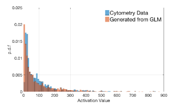
In this section we give further details on the flow cytometry experiments. As detailed in the main paper we use the causal graph in Fig. 5(c) in [26] (shown in Fig. 3a) as the ground truth. Then we fit a GLM gamma model [14] between each node in the graph and its parents using the observational data-set. The GLM model produces a highly accurate representation of the flow cytometry data-set. In Fig. 11a we plot the histogram for the activation of an internal node pip2 from the real data and samples generated from the GLM probabilistic model. It can be seen that the histograms are very close to each other.

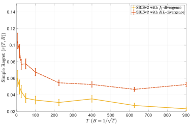
In Fig. 11b we plot the performance of SRISv2 when the divergence metric is replaced by $\mathrm{KL}$-divergence. In one of the plots SRISv2 is modified by setting $M_{ij}=1+\mathrm{KL}(P_{i}||P_{j})$. It can be seen that the performance degrades, which signifies that our divergence metric is fundamental to the problem.

(a)

(b)

Figure 11: Illustration of our experimental methods.

D.2 More on Interpretation of Inception Deep Network

In this section we describe the methodology of our model interpretation technique in more detail. In Section 4.2 we have described how the best arm algorithm can be used to pick a distribution over the superpixels of an image, that has the maximum likelihood of producing a certain classification from Inception. Here, we describe how the distributions over the superpixels are generated and how they are used subsequently. The arm distributions are essentially points in the $n$-dimensional simplex (where $n$ is the number of superpixels into which the image is segmented). These distributions are generated in a randomized fashion using the following methods:

1. Generate a point uniformly at random in the $n$-dimensional simplex.

2. Randomly choose $l<n$ superpixels. Make the distribution uniform over them and $0$ elsewhere.

3. Randomly choose $l<n$ superpixels. The probability distribution is a uniformly chosen random point over the $l$-dimensional simplex with support on the $l$ chosen superpixels and $0$ elsewhere.

4. Start a random walk from a few superpixels which traverses to adjacent superpixels at each step. Stop the random-walk after a certain number of steps and choose the superpixels touched by the random walk. Then choose a uniform distribution over the super pixel support or choose a random distribution from the simplex of probability distributions over the support of the chosen superpixels (like in the previous point) and $0$ elsewhere. This method uses the geometry of the image.

Note that all the above methods do not depend on the specific content of the images. Using the above methods $L$ pull arms are chosen which are used to collect the rewards. Further there are $K$ opt arms that are the interventions to be optimized over. When an arm is used to sample, then $m\ll n$ superpixels are chosen with replacement from the distribution of that arm. These pixels are preserved in the original image while everything else is blurred out before feeding this into the neural network. Thus if the distribution corresponding to an arm is $P$, then the actual distribution to be used for the importance sampling is the product distribution $P^{m}$. Note that the pull arms are separate from the opt arms. The true counterfactual power of our algorithm is showcased in this experiment, as we are able to optimize over a large number of interventions that are never physically performed.

References

- [1] Jacob Abernethy, Yiling Chen, Chien-Ju Ho, and Bo Waggoner. Low-cost learning via active data procurement. In Proceedings of the Sixteenth ACM Conference on Economics and Computation, pages 619–636. ACM, 2015.
- [2] Radhakrishna Achanta, Appu Shaji, Kevin Smith, Aurelien Lucchi, Pascal Fua, and Sabine Süsstrunk. Slic superpixels. Technical report, 2010.
- [3] Jean-Yves Audibert and Sébastien Bubeck. Best arm identification in multi-armed bandits. In COLT-23th Conference on Learning Theory-2010, pages 13–p, 2010.
- [4] George Bennett. Probability inequalities for the sum of independent random variables. Journal of the American Statistical Association, 57(297):33–45, 1962.
- [5] Hubert M Blalock. Causal models in the social sciences. Transaction Publishers, 1985.
- [6] Richard Bonneau, Marc T Facciotti, David J Reiss, Amy K Schmid, Min Pan, Amardeep Kaur, Vesteinn Thorsson, Paul Shannon, Michael H Johnson, J Christopher Bare, et al. A predictive model for transcriptional control of physiology in a free living cell. Cell, 131(7):1354–1365, 2007.
- [7] Léon Bottou, Jonas Peters, Joaquin Quinonero Candela, Denis Xavier Charles, Max Chickering, Elon Portugaly, Dipankar Ray, Patrice Y Simard, and Ed Snelson. Counterfactual reasoning and learning systems: the example of computational advertising. Journal of Machine Learning Research, 14(1):3207–3260, 2013.
- [8] Alexandra Carpentier and Andrea Locatelli. Tight (lower) bounds for the fixed budget best arm identification bandit problem. arXiv preprint arXiv:1605.09004, 2016.
- [9] Image source. http://bit.ly/2hviIwP. Accessed: 2017-02-23.
- [10] Lijie Chen and Jian Li. On the optimal sample complexity for best arm identification. arXiv preprint arXiv:1511.03774, 2015.
- [11] Hyunghoon Cho, Bonnie Berger, and Jian Peng. Reconstructing causal biological networks through active learning. PloS one, 11(3):e0150611, 2016.
- [12] Frederick Eberhardt. Almost optimal intervention sets for causal discovery. In Proceedings of 24th Conference in Uncertainty in Artificial Intelligence (UAI), pages 161–168, 2008.
- [13] Victor Gabillon, Mohammad Ghavamzadeh, and Alessandro Lazaric. Best arm identification: A unified approach to fixed budget and fixed confidence. In Advances in Neural Information Processing Systems, pages 3212–3220, 2012.
- [14] James William Hardin, Joseph M Hilbe, and Joseph Hilbe. Generalized linear models and extensions. Stata press, 2007.
- [15] Alain Hauser and Peter Bühlmann. Two optimal strategies for active learning of causal networks from interventional data. In Proceedings of Sixth European Workshop on Probabilistic Graphical Models, 2012.
- [16] Antti Hyttinen, Frederick Eberhardt, and Patrik Hoyer. Experiment selection for causal discovery. Journal of Machine Learning Research, 14:3041–3071, 2013.
- [17] Kevin G Jamieson, Matthew Malloy, Robert D Nowak, and Sébastien Bubeck. lil’ucb: An optimal exploration algorithm for multi-armed bandits. In COLT, volume 35, pages 423–439, 2014.
- [18] Michael Joffe, Manoj Gambhir, Marc Chadeau-Hyam, and Paolo Vineis. Causal diagrams in systems epidemiology. Emerging themes in epidemiology, 9(1):1, 2012.
- [19] Emilie Kaufmann, Olivier Cappé, and Aurélien Garivier. On the complexity of best arm identification in multi-armed bandit models. The Journal of Machine Learning Research, 2015.
- [20] Patrick Kemmeren, Katrin Sameith, Loes AL van de Pasch, Joris J Benschop, Tineke L Lenstra, Thanasis Margaritis, Eoghan O?Duibhir, Eva Apweiler, Sake van Wageningen, Cheuk W Ko, et al. Large-scale genetic perturbations reveal regulatory networks and an abundance of gene-specific repressors. Cell, 157(3):740–752, 2014.
- [21] Gabriel Krouk, Jesse Lingeman, Amy Marshall Colon, Gloria Coruzzi, and Dennis Shasha. Gene regulatory networks in plants: learning causality from time and perturbation. Genome biology, 14(6):1, 2013.
- [22] Finnian Lattimore, Tor Lattimore, and Mark D Reid. Causal bandits: Learning good interventions via causal inference. In Advances In Neural Information Processing Systems, pages 1181–1189, 2016.
- [23] Lihong Li, Wei Chu, John Langford, and Xuanhui Wang. Unbiased offline evaluation of contextual-bandit-based news article recommendation algorithms. In Proceedings of the fourth ACM international conference on Web search and data mining, pages 297–306. ACM, 2011.
- [24] Po-Ling Loh and Peter Bühlmann. High-dimensional learning of linear causal networks via inverse covariance estimation. Journal of Machine Learning Research, 15(1):3065–3105, 2014.
- [25] Nicolai Meinshausen, Alain Hauser, Joris M Mooij, Jonas Peters, Philip Versteeg, and Peter Bühlmann. Methods for causal inference from gene perturbation experiments and validation. Proceedings of the National Academy of Sciences, 113(27):7361–7368, 2016.
- [26] Joris Mooij and Tom Heskes. Cyclic causal discovery from continuous equilibrium data. arXiv preprint arXiv:1309.6849, 2013.
- [27] Joris M Mooij, Jonas Peters, Dominik Janzing, Jakob Zscheischler, and Bernhard Schölkopf. Distinguishing cause from effect using observational data: methods and benchmarks. Journal of Machine Learning Research, 17(32):1–102, 2016.
- [28] Judea Pearl. Causality. Cambridge university press, 2009.
- [29] Judea Pearl. Causality: Models, Reasoning and Inference. Cambridge University Press, 2009.
- [30] Fernando Pérez-Cruz. Kullback-leibler divergence estimation of continuous distributions. In Information Theory, 2008. ISIT 2008. IEEE International Symposium on, pages 1666–1670. IEEE, 2008.
- [31] Marco Tulio Ribeiro, Sameer Singh, and Carlos Guestrin. Why should i trust you?: Explaining the predictions of any classifier. In Proceedings of the 22nd ACM SIGKDD International Conference on Knowledge Discovery and Data Mining, pages 1135–1144. ACM, 2016.
- [32] Karen Sachs, Omar Perez, Dana Pe’er, Douglas A Lauffenburger, and Garry P Nolan. Causal protein-signaling networks derived from multiparameter single-cell data. Science, 308(5721):523–529, 2005.
- [33] Karthikeyan Shanmugam, Murat Kocaoglu, Alexandros G Dimakis, and Sriram Vishwanath. Learning causal graphs with small interventions. In Advances in Neural Information Processing Systems, pages 3195–3203, 2015.
- [34] Aleksandrs Slivkins. Dynamic ad allocation: Bandits with budgets. arXiv preprint arXiv:1306.0155, 2013.
- [35] Peter Spirtes, Clark Glymour, and Richard Scheines. Causation, Prediction, and Search. A Bradford Book, 2001.
- [36] Jerzy Splawa-Neyman, DM Dabrowska, TP Speed, et al. On the application of probability theory to agricultural experiments. essay on principles. section 9. Statistical Science, 5(4):465–472, 1990.
- [37] Masashi Sugiyama, Matthias Krauledat, and Klaus-Robert MÞller. Covariate shift adaptation by importance weighted cross validation. Journal of Machine Learning Research, 8(May):985–1005, 2007.
- [38] Christian Szegedy, Wei Liu, Yangqing Jia, Pierre Sermanet, Scott Reed, Dragomir Anguelov, Dumitru Erhan, Vincent Vanhoucke, and Andrew Rabinovich. Going deeper with convolutions. In Proceedings of the IEEE Conference on Computer Vision and Pattern Recognition, pages 1–9, 2015.
- [39] Tong Zhang and Peiling Zhao. Stochastic optimization with importance sampling for regularized loss minimization. arXiv preprint arXiv:1401.2753, 2014.