Measurements of Solar Differential Rotation and Meridional Circulation from Tracking of Photospheric Magnetic Features

Abstract

Long-lived rotational and meridional flows are important ingredients of the solar cycle. Magnetic field images have typically been used to measure these flows on the solar surface by cross-correlating thin longitudinal strips or square patches across sufficiently long time gaps. Here, I use one month of SDO/HMI line-of-sight magnetic field observations, combined with the SWAMIS magnetic feature tracking algorithm to measure the motion of individual features in these magnetograms. By controlling for perturbations due to short-lived flows and due to false motions from feature interactions, I effectively isolate the long-lived flows traced by the magnetic features. This allows me to produce high-fidelity differential rotation measurements with well-characterized variances and covariances of the fit parameters. I find a sidereal rotational profile of $(14.296\pm 0.006)+(-1.847\pm 0.056)\sin^{2}b+(-2.615\pm 0.093)\sin^{4}b$, with units of $\textrm{ deg d}^{-1}$, and a large covariance $\sigma_{BC}^{2}=-4.87\times 10^{-3}(\textrm{ deg d}^{-1})^{2}$. I also produce medium-fidelity measurements of the much weaker meridional flow that is broadly consistent with previous results. This measurement shows a peak flow of $16.7\pm 0.6\text{ m s}^{-1}$ at latitude $b=45\degree$ but is insufficiently characterized at higher latitudes to ascertain whether the chosen functional form $2\cos b\sin b$ is appropriate. This work shows that measuring the motions of individual features in photospheric magnetograms can produce high precision results in relatively short time spans, and suggests that high resolution non-longitudinally averaged photospheric velocity residual measurements could be produced to compare with coronal results, and to provide other diagnostics of the solar dynamo.

1 Introduction

Long-lived photospheric flows are important drivers and diagnostics of the dynamo that is responsible for the solar cycle. Both flows are now thought to be direct consequences of the convection that occurs in the outer $\sim$30% of the Sun by radius (Miesch et al., 2008, e.g.,, particularly §4). On a global scale the rotational (alternatively longitudinal or zonal) flow, converts poloidal magnetic field into toroidal magnetic field. The meridional (alternatively latitudinal) flow is an essential component of some tools for studying the solar magnetic cycle that invoke the Babcock-Leighton mechanism (Babcock, 1961; Leighton, 1964, 1969) such as surface-flux transport simulations (e.g., Yeates et al., 2007; Sheeley, 2005) and flux-transport dynamo models (see Choudhuri, 2015, for a recent critical assessment), though perhaps not all models require this flow (Charbonneau, 2010, §6.5). Thus understanding the nature of both the rotational and meridional flows in the solar interior and on the surface is important for advancing our understanding of the solar dynamo.

The rotational flow varies with latitude, depth (Thompson et al., 1996), and time (Gilman & Howard, 1984); variations in the flow are strongly linked to the appearance and location of active regions and the phase of the solar cycle (Howard & Labonte, 1980). Besides these solar effects, measurements of solar rotation can also vary for systematic reasons, most prominently the use of different measurement techniques and methods. Beck (2000) provides a review of the measurement techniques and their results through the end of the 20th century. Spectroscopic observations of the plasma doppler shift at the limb (Howard et al., 1983) yield different results from observations of surface tracers, and the rotation curves from different kinds of tracers are as different as the tracers themselves (a canonical example is Cox, 2000, Table 14.25, and references therein). It is for these reasons that despite decades (or centuries) of study, what exactly is meant by the “solar differential rotation rate” is subject to considerable ambiguity. Some of these differences might be attributable to physical causes such as the different depths at which the tracers are anchored. Other differences likely arise from poorly understood or uncorrected systematic effects. Separating physical effects from systematic effects is important to the interpretation of the measurements: if, for example, a coronal hole pattern rotates at a different rate than the underlying magnetic field, this may require an interpretation in which magnetic reconnection is constantly occurring at the coronal hole boundary; conversely, if the measured differences arise due to differences in the definition of the boundary or to difficulties localizing the boundary in three-dimensional space, then a topologically static coronal hole boundary may be the best interpretation. Therefore, exploring the rotational rate measured by different solar features and methods can still provide useful insight into basic solar processes, nearly 400 years after solar differential rotation was discovered.

The meridional flow also varies with latitude, depth, and time, though because this flow is 2–3 orders of magnitude slower than the rotational flow, its basic structure is still a matter of debate. While the poleward flow at low and medium latitudes is well-established, it has not been conclusively settled whether the flow continues all the way to the pole, or instead a meridional flow counter-cell exists at high latitudes. The structure of the flow as a function of depth in the convection zone is even more uncertain, with some measurements supporting a single cell having a surface poleward flow and a deep equator-ward return flow, and others supporting more than one cell, with a surface and deep poleward flows and an equator-ward return flow at shallower depths in the convection zone (Rightmire-Upton et al., 2012; Zhao et al., 2013; Komm et al., 2015; Rajaguru & Antia, 2015).

Surface measurements of these flows are accomplished via a variety of methods: direct measurement of the Doppler shift of a spectral line, the motion of magnetic field tracers such as sunspots, the small-scale magnetic pattern, and faculae. The rotation has also been measured in the corona, using for example coronal holes or coronal bright points. The values of the rotational and meridional flows produced by a single method vary over time, which is assumed to be due to solar effects. However, while there is a lack of agreement between the various methods, making meaningful comparisons between the different methods is difficult, because of the solar effects as well as the systematic effects introduced due to different quantities being measured and different measurement techniques. One must also consider the possibility that some “systematic” effects may in fact be solar, e.g., the difference between the true rotation rate of sunspots and small magnetic features may well be solar in origin.

In the past, precise measurements of even the rotational speed typically required long time periods of measurement, due to a combination of low data cadence, low spatial resolution, and the need for a statistically significant number of samples across a wide range of solar latitudes. A typical technique in photospheric measurements has been to divide the surface into patches, either roughly square (Howard et al., 1990) or rectangular longitudinal strips (Hathaway & Rightmire, 2010), and perform a cross-correlation of those patches over some time lag ($\sim 8$ hrs or $\sim 1$ day). Accurately measuring the motion due to individual elements has been difficult for the same reasons of cadence, resolution, and statistics. A recent commendable attempt to acquire a precise measurement of the rotation profile in the solar corona with only a 2-day dataset, using 906 coronal bright points as tracers, was made by Sudar et al. (2015), and was the inspiration for the present work. However, note that even with wide (5 degree) latitudinal bins, there was still significant scatter about their line of best fit (see their Figures 6 & 7). A much larger coronal bright point dataset was used by Sudar et al. (2016), to which I return at the end of the paper.

In this paper I measure the solar photospheric rotational and meridional flows using measurements of the motion of individual magnetic features. I use approximately one month of high cadence SDO/HMI observations of the line-of-sight photospheric magnetic field, and track the positions of the features using a well-tested feature-tracking algorithm. After filtering to remove the effect of evolution due to short-lived flows, I produce measurements of the average rotational and meridional flows derived from these magnetic features over this one-month time period. The rotational measurements have a high latitudinal resolution (2°) and are precise, with no significant deviation from the line of best fit. The values of the fitting parameters approximately agree with previous work, with well-characterized variances and covariances. The weaker meridional motion is in rough agreement with previous measurements of the poleward surface flow, though the measurement is noisier than the rotational motion when using the same dataset, as expected. The novel measurement technique presented here opens the future possibility to measuring non-longitudinally-averaged rotational flows, and high-fidelity meridional flows with longer data sets.

In §2 I describe the data and observations, which includes the methods of measuring the flows. In §3 I perform fits of analytic functions to both the rotational and meridional measurements, which includes estimates of the errors in the fit parameters. In §4 I present my conclusions, including the possibility of future measurements using this technique.

2 Data & Observations

I used a series of line-of-sight magnetograms from the Helioseismic and Magnetic Imager (Scherrer et al., 2012) aboard the Solar Dynamics Observatory (Pesnell et al., 2012). The magnetograms were retrieved from the near-real-time 45 s magnetogram data series at a cadence of 12 min. The dataset comprises 3000 images beginning at 2011-02-01T00:00:45 TAI and ending at 2011-02-26T08:24:45 TAI. There are 23 instances of missing frames in the dataset: 17 are gaps of a single frame, and the remainder are gaps of 2, 2, 4, 5, 5, and 8 frames. I address the issue of data gaps later in this section.

Preprocessing includes rotation of each image by $180\degree$ so that solar north is “up”, and for reasons of computational efficiency reducing the spatial size of the original data by a factor of 4. Size reduction is accomplished using an optimized filter with a Hanning ($\cos^{2}$) rolloff (DeForest, 2004). The reduced images are $1024\times 1024$ pixels, with an angular scale of 2.0” per pixel, which is sufficient for these purposes. The input magnetograms were corrected for magnetic field vector line-of-sight effects, assuming that the magnetic field is vertical at the photosphere, a small variation on the technique first used by Hagenaar (2001). This is an acceptable assumption away from active regions where I perform most of the analysis in this paper (but see Leka et al., 2013 for an alternative correction that assumes the fields are potential). For simplicity, I do not use vector magnetogram information in the active regions—the contribution from active regions to my measurements turns out to be nearly negligible. The line-of-sight correction takes the form of dividing the line-of-sight flux density in each pixel by $\cos(\alpha)$, $\alpha=\eta+\delta,$ where $\eta$ is the Sun-centered angle subtended by the great circle segment connecting each pixel to the disk image center, and $\delta$ is the (small) angle between a line connecting a given pixel to the observer and a line from that pixel that is parallel to the line connecting Sun center to the observer (Figure 1).

Figure 1: Illustration of the line-of-sight correction geometry. The angle $\eta$ subtends the photospheric arc connecting the sub-observer point $\mathcal{O}$ and a given location $\mathcal{P}$ as viewed from the center of the Sun. The angle $\delta$ subtends these same two points as viewed from the observer. $\alpha=\eta+\delta$ is the angle between local vertical and the line connecting the observer and $P$. The drawing is not to scale: for an observer at 1 AU $\delta\lessapprox 0.25\degree$ and $0\leq\eta\lessapprox 90\degree$. The corrections to produce the field and flux images involve dividing the input magnetogram by $\cos(\alpha)$ and $\cos^{2}(\alpha)$, respectively.

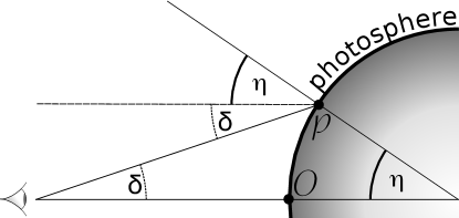
Assuming the magnetic field vector is vertical in the region of the photosphere where the magnetograms are observed, division by $\cos(\alpha)$ fully corrects for the discrepancy between local vertical and the line-of-sight. The image produced by this correction is called the field image. The field image is again divided by $\cos(\alpha)$ to correct for foreshortening: the increase between disk center and limb in the solar surface area subtended by a pixel. The image produced by this correction is called the flux image. The field and flux images are cropped so that all pixels for which $\alpha\geq 70\degree$ are ignored in subsequent processing.

The prepared data were then processed by the Southwest Automatic Magnetic Identification Suite (SWAMIS) feature tracking algorithm (DeForest et al., 2007), and I refer the reader to that work for a detailed description of the methodology and terminology. SWAMIS is five-step algorithm that identifies magnetic features on the solar surface and associates them across multiple images. Magnetic features are regions of the solar surface, grouped into collections of adjacent pixels that all have a pixel-averaged field strength above a certain low threshold, and that have at least one pixel above a certain high threshold at some point in time. A feature must also satisfy certain nominal minimum size and lifetime requirements in order to make the detections robust against different sources of noise.

In the discrimination step, I used a high detection threshold of 53 G and a low detection threshold of 15 G on the field images. In the identification step, I used a hybrid combination of the “downhill” and “clumping” methods, with the clumping method applied to pixels above a 33 G threshold, and the downhill method applied to pixels below that threshold. I measured the noise in the scaled-down magnetograms (as in Hagenaar et al., 1999) to be approximately 5.2 G, so these three thresholds correspond to approximately 10, 3, and 6.5 $\sigma$ respectively.

Association of features between sequential flux images was performed with the dual-maximum flux-weighted overlap method described by (DeForest et al., 2007). The association algorithm makes the identification number of each feature unique across the dataset, which enables my image-to-image velocity calculations. It is important to note that the association algorithm employed here makes no attempt to account for rotational motion when associating features between images, so understanding the performance of this step across data gaps is important. I made a visual comparison between identified features before and after various-sized gaps, and found that the association step performs acceptably well on my scaled-down data over data gaps $\leq$ 8 images (96 min). Over larger data gaps the rotational motion moves features too far for direct association to be accurate, and the mistaken identity problem manifests–a feature will be incorrectly associated across the gap if an unrelated feature of the same polarity happens to be present at the same location after the data gap. After the association step, the tabulation step accumulates data for each feature in each image into a feature table that contains the flux, area, flux-weighted centroid location, and the identification number of features that are considered to be neighbors of this feature, among other quantities. The neighbors of a feature are those features found within a two-pixel boundary around each feature. If a feature has neighbors in a given image, I set a closeness parameter to 1 for that feature in that image. After the feature table has been made, a summary table is made that has summary information for each feature across all images: birth and death images numbers, lifetime, and the average closeness. In total, $7.85\times 10^{6}$ features are present in the dataset; the lifetime and average closeness quantities are used to filter features in the remainder of this paper (§§2.1.2 & 2.2).

2.1 Longitudinal Flow Measurement

2.1.1 The Synodic-Sidereal Correction

After tracking, the features’ pixel locations stored in the feature table are converted heliographic coordinates (central meridian distance $l$ and latitude $b$) using a perspective transformation for each image. For each feature, I used equations (1) and (2) of Sudar et al. (2015) to estimate $\omega_{syn}$ and $\omega_{mer}$. Those equations are the ordinary least squares estimates of $\omega_{syn}$ and $\omega_{mer}$ using a simple regression model. To convert the synodic rotation rate $\omega_{syn}$ to the sidereal rotation rate $\omega_{sid}$ I also used equation (7) of Skokić et al. (2014):

$$\omega_{sid}=\omega_{syn}+\frac{\bar{\omega}_{Earth}}{r^{2}}\frac{\cos^{2}\Psi}{\cos i}.$$ (1)

In that equation, $\bar{\omega}_{Earth}=0.9856\text{ deg}\textrm{ d}^{-1}$ is Earth’s yearly-averaged angular speed, $r$ is the dimensionless Earth-Sun distance expressed in AU, $i$ is the inclination of the solar equator to the ecliptic, and $\Psi$ is the angle between the pole of the ecliptic and the solar rotation axis orthographically projected onto the solar disk. The first fraction $\frac{\bar{\omega}_{Earth}}{r^{2}}$ gives Earth’s instantaneous angular speed $\omega_{Earth}$. In the second fraction, $\Psi$ is calculated from

$$\tan\Psi=\tan i\cos(\lambda_{0}-\Omega),$$ (2)

where $\lambda_{0}$ is the apparent longitude of the Sun with respect to the true equinox on the date of observation, and $\Omega$ is the longitude of the ascending node of the solar equator on the ecliptic. The quantities $r$ and $\lambda_{0}$ can be retrieved from the the JPL Horizons ephemerides by selecting the Observer ephemeris type and including the “Observer range & range-rate” and the “Observer ecliptic lon. & lat.” output quantities, respectively. For $i$ I use 7.25°, and for $\Omega=73\degree 40^{\prime}+50.25"(t-1850.0)$, where $t$ is the time expressed in fractional years (Roša et al., 1995). As an example, for 2011-Feb-01 00:00:00 UTC, $r=0.9853$, thus $\lambda_{0}=311.76\degree$, and $\Omega=75.92\degree$. Thus $\Psi=-4.0852\degree$, $\cos^{2}(\Psi)/\cos(i)=1.002942$. $\omega_{Earth}=1.01523\text{ deg}\textrm{ d}^{-1}$ and thus the difference between the calculated sidereal and measured synodic rotation rates is $1.018215\text{deg}\,\textrm{d}^{-1}$. As a check, I note that this is faster than average $(\bar{\omega}_{Earth})$ because Earth is near perihelion in February. For a feature first detected at this time with $\omega_{syn}=12.170066\text{ deg}\,\text{d}^{-1}$, I thus compute $\omega_{sid}$ to be $13.188281\text{ deg}\,\text{d}^{-1}$.

2.1.2 Magnetic Feature Selection and Filtering

Magnetic features are subject to motion by a bevy of plasma flows. At the 12 min data cadence used here, granulation flows changing on time scales of 5–10 minutes act to buffet the features, while super- and (perhaps) meso-granular flows can act to produce sustained feature motions over $\sim$24 h and 0.5-4 h respectively. In addition to these flows, interactions among features can cause apparent motion of the feature centroids. During a merging of two like-signed features, the feature with the larger flux retains its identification number (assured by the dual flux-weighted overlap criterion of the feature tracking’s association step), so the addition of flux from the smaller feature can cause the flux-weighted centroid location of the larger feature to jump in the direction of the smaller feature after the merge. Therefore understanding and controlling for the effect of feature interactions is an important step in separating systematic from real effects.

I use two parameters to control the number of features in the ensemble used for measuring the rotational flow $\omega_{sid}$: the lifetime, and the average closeness of each feature. The rotational measurement is largely insensitive to the choice of parameters, but there are some combinations that provide smaller error bars and smoother average rotational profiles than others, as shown below. I created ensembles of features that had lifetimes greater than certain thresholds, and average closeness less than certain thresholds. In general, if the thresholds are made excessively strict then insufficient numbers of features are available for averaging and even the fact that the Sun rotates differentially can not be conclusively determined. If the thresholds are made too lenient other processes such as the aforementioned merging substantially affect the measurement.

The feature lifetime distribution is steep and dominated by features with short lifetimes (Figure 2), and fragmentation and merging are the dominant methods of feature birth and death (Lamb et al., 2013).

Figure 2: Lifetime distribution of features in the data set, in a single 20–22° N latitudinal bin, with a 1-frame binning. No correction has been made for the data gaps, which would result in a small shift to the right of some of the features. Note that both axes are logarithmically scaled.

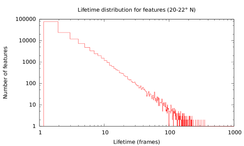
Because of this, an ensemble with a short lifetime threshold will include many features that are born and die by these methods. The recorded birth and death frame of each feature are the frames in which the feature is first or last recognized, and not instead the frame in which the interaction that resulted in the birth or death was first determined to begin. Since the interactions may take multiple frames to complete, the linear fit of the feature’s position over time (equations (1) & (2) of Sudar et al. (2015)) can be strongly affected by the birth and death interactions if the lifetime threshold is chosen to be too low. In addition, making the average closeness threshold less strict allows for more feature-feature interactions, and thus the position of the flux-weighted centroid of a feature experiencing an interaction undergoing merging will have large jumps that are not due to the flow but rather to these interactions. The surface density of coronal bright points ($\sim$100 on the disk at any one time) is two orders of magnitude lower than the average surface density of magnetic features, so the average closeness threshold should be set so as to exclude those features that are always nearby (and presumably interacting with) other features.

Figure 2.1.2

Rotational motion for lifetime (rows; top to bottom: 10, 50, 100) and average closeness parameters (columns; left to right: 0.15, 0.50, 1.00). The latitudinal bin size in all plots is 2 degrees. The combination of the lifetime and average closeness parameters strongly affects the smoothness of the mean profiles and the width and symmetry of the distributions in the latitudinal bins. I use the boxed plot for the rotational profile analysis in the remainder of the paper. shows rotational flow measurements for all combinations of lifetime $\geq$ (10, 50, 100) frames and average closeness $\leq$ (0.15, 0.5, 1.0). For lifetime $\geq$ 100 and average closeness $\leq$ 0.15 (lower-left panel), I am selecting features that live $\geq$ 20 hours and have a neighboring feature less than 15% of the time. Since even the supergranular network turns over on timescales of $\sim$24 h, and the average closeness threshold excludes feature-dense regions such as active regions, it is not surprising that only 43 features satisfy these criteria, making even a measurement of the rotational motion unreliable. On the opposite end of the range (upper right panel), I find that changing the selection thresholds so as to include the largest number of features is not necessarily desirable. For lifetime $\geq$10 frames and average closeness $\leq 1$ (i.e., no restriction), over $5\times 10^{5}$ features are found. Even though the 2$\sigma$ error bars are very small, the median of each bin is much higher from the mean than those error bars–a large number of low velocity features depress the mean from the median in each bin–and the distributions are much wider than would be expected on physical grounds. That the low-velocity tail so substantially affects the mean suggests that suggests that additional filtering of features is necessary in order to bring the mean and median into closer agreement and reduce the outsize effect of the tails of the distribution in each latitudinal bin.

Sudar et al. (2015) discarded any bright points with sidereal speeds $\leq 8$ or $\geq 19\mbox{ deg}\text{ d}^{-1}$. I can explicitly discard those features, or achieve the same results (while also potentially discarding a small number of desirable features) by using a lifetime threshold of at least 28 frames (5.6 h). Over the range of lifetime thresholds between 30 and 100 frames the mean of the sidereal rotation between 20 and 22°latitude differs only by $0.2\text{ deg}\text{ d}^{-1}$, the median only by $0.13\text{ deg}\text{ d}^{-1}$. The difference between the two, which is indicative of asymmetries in the velocity distributions, is less than $0.1\text{ deg}\text{ d}^{-1}$ over this range (Table 1). For the remainder of the rotational flow results, I adopt a minimum lifetime of 50 frames as a reasonable compromise between rejecting outliers and having a large enough sample size in each bin. It is at this point in Table 1 that the difference between the mean and median in that particular latitudinal bin first reaches a local minimum.

Table 1: Mean and median sidereal rotation velocities, and their difference, and the number of features, for features with $20\degree\leq b\leq 22\degree$ and given minimum lifetime thresholds.

Min Lifetime (frames)	Mean $(\degree\text{d}^{-1})$	Median $(\degree\text{d}^{-1})$	Difference $(\degree\text{d}^{-1})$	N
10	13.263	13.716	0.453	9426
20	13.812	13.936	0.124	3768
30	13.912	13.991	0.080	2211
40	13.974	14.031	0.058	1496
50	14.031	14.059	0.028	1101
60	14.040	14.074	0.035	829
70	14.067	14.098	0.031	650
80	14.077	14.099	0.022	524
90	14.089	14.099	0.010	424
100	14.110	14.127	0.017	365

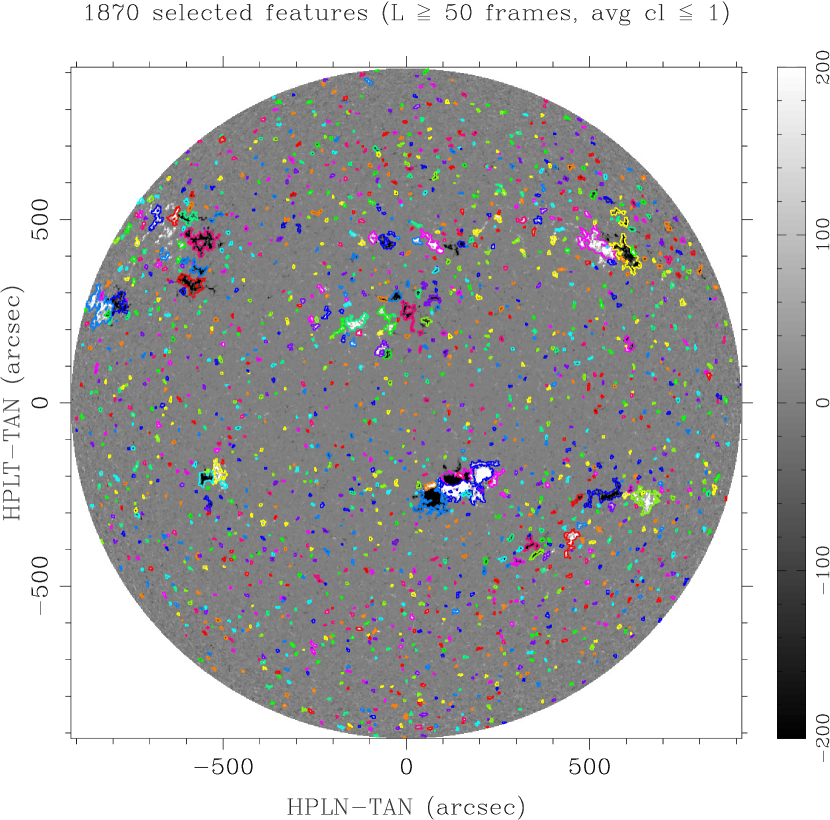
For the 50-frame lifetime threshold, I also produced plots like those in Figure 2.1.2 for average closeness thresholds of 0.8 and 0.9. Even though those thresholds excluded active regions but the threshold of 1.0 includes active regions, I find no substantial difference in the rotational profile. For a threshold of 1.0, the rotation profile is essentially unchanged at the active latitudes, and is smoother at higher absolute latitudes (due to larger number of features). Thus for the remainder of the rotational flow analysis, I adopt the parameters of (lifetime $\geq$ 50 frames, average closeness $\leq$ 1.0). Figure 3 shows the features selected by these parameters for a single magnetogram.

Figure 3: Magnetogram from 2011-02-14 17:36:45 TAI with the 1870 features that are identified by SWAMIS in that frame and that satisfy my parameter thresholds (lifetime $\geq$ 50 frames, average closeness $\leq$ 1.0). The colors of the feature outlines are for clarity only; similarities or differences among them carry no scientific meaning. Pixels where $\alpha\geq 70\degree$ have been cropped out, as described in the § 2 text. The magnetogram grayscale saturates as $\pm 200$ G.

2.2 Latitudinal Flow Measurement

Because the meridional flow is 2–3 orders of magnitude slower than the rotational flow, by all methods used to date it is more difficult to measure and has larger uncertainties than rotational flow measurements. Figure 2.2

Similar to Figure 2.1.2, but for the features’ meridional speed given lifetime thresholds (rows; top to bottom: 10, 50, 100) and average closeness parameters (columns; left to right: 0.15, 0.50, 1.00). Again, the combination of the lifetime and average closeness parameters strongly affects the smoothness and apparent functional form of the mean profiles and the width and symmetry of the distributions in the latitudinal bins. shows the meridional flow measurement for the same combination of lifetime and average closeness thresholds as in Figure 2.1.2. For the measurement of the meridional velocities, I note again that several combinations of thresholds results in curves that are too noisy to be meaningful: all measurements for which average closeness $\leq 0.15$, (100, 0.5), and (50, 0.5). Combinations (10, 0.5) and (10, 1) are noticeably different from (50,1) & (100, 1): the former two have very high speeds at high latitudes, with no evidence of the mid-latitude peak in the meridional speed that is seen to some degree in the latter two observations. That peak seems to suggest a functional form of $\omega_{mer}\propto 2\sin\theta\cos\theta$ (Hathaway & Rightmire, 2010), though I must understand the difference between the two trends and not simply choose the one that matches other observations. Considering the difference between (50, 1) and (10,1), the latter includes 10 times as many features, and the excess features all have lifetimes between 10 and 49 frames. As for the rotational flow, the mean and median of each bin do not agree, particularly in the higher latitudes, similar to how the mean and median rotational flow did not agree for some parameter combinations. I again examine the difference between the mean and median in the bins. Because of the noisier plots I calculate the mean and median of each 2-degree-wide bin in the range 20°–30° N. Table 2 shows the mean of the bin means, the mean of the bin medians, and the mean of the absolute value of their differences, as a function of lifetime threshold.

Table 2: Mean and median meridional flow velocities, and their difference, and the number of features, for features with $20\degree\leq b\leq 30\degree$ divided into 2°bins and given minimum lifetime thresholds.

Min Lifetime (frames)	<Mean> $(\text{m/s})$	<Median> $(\text{m/s})$	<|Difference|> $(\text{m/s})$	N
10	35.582	25.911	9.671	44328
20	23.472	18.408	5.065	17350
30	18.243	15.060	3.183	10097
40	15.346	12.449	2.969	6813
50	13.825	11.781	2.611	5044
60	14.094	12.069	2.745	3813
70	13.233	11.731	2.499	2996
80	13.162	11.725	2.497	2445
90	13.246	11.845	2.259	2002
100	14.151	12.049	2.840	1658

Again, the difference between the mean of the bin means and the mean of the bin medians has its first local minima at a lifetime threshold of 50 frames, as for the lifetime distributions.

At the 50-frame lifetime threshold, I examined the effect of the average closeness threshold. Here the effect seems to be much more pronounced than for the rotational flow, especially for the highest northern latitudes measured in this February dataset. In particular, the peak at $\sim$45° N shown in Figure 2.2 disappears when the average closeness threshold is reduced from 1.0 to 0.9. Figure 2.2 compares the effect of the two thresholds on the measured profile. (a) (b) (c)

Effect of the average closeness threshold on the meridional flow profile. For a lifetime threshold of 50 frames and average closeness of (a) 0.9 and (b) 1.0. Panel (b) is the same data as the right middle panel of Figure 2.2, but with a reduced velocity axis range. (c) Similar to Figure 3, but for an average closeness of 0.9. The most obvious effect is that the active region features are no longer selected, but a closer inspection reveals features in the quiet sun that are excluded as well.

I return to the effect of the choice of average closeness threshold in §3.2.

3 Analytic Function Fits

3.1 Longitudinal Flow

I used a Levenberg-Marquardt least squares routine to fit the sidereal rotational velocities to the commonly-used function

$$\omega_{sid}=A+B\sin^{2}b+C\sin^{4}b.$$ (3)

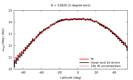
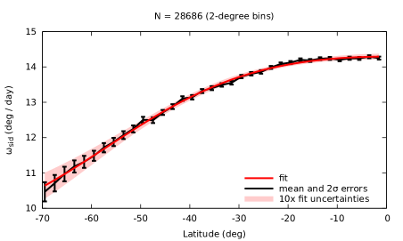
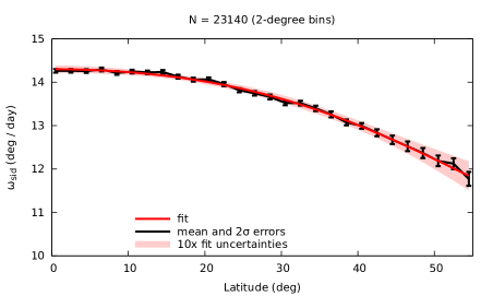
Best-fit values of the parameters A, B, and C, as well as the covariance matrix for these three parameters, is shown in Table 3 (the bottom triangle of the symmetric covariance matrix is not shown for clarity). It is well-known that significant cross-talk exists between the parameters $B$ and $C$, because $\sin^{2}b$ and $\sin^{4}b$ are not orthogonal functions. This cross-talk is evidenced by the large (negative) value of $\sigma_{BC}^{2}$ in Table 3—an increase in $B$ could result in a decrease in $C$ without substantially affecting the overall quality of the fit. Figure 4 shows the mean of the observations, the fit from Table 3, and the estimate of the errors in the fit from the covariances (increased by a factor of 10 for visibility). Errors in the fit are calculated using a standard error propagation formula (Bevington & Robinson, 2003, Chapter 3), which in this case is

$$s_{sid}^{2}(b)=\sigma_{A}^{2}+\sigma_{B}^{2}\sin^{4}b+\sigma_{C}^{2}\sin^{8}b+2\sigma_{AB}^{2}\sin^{2}b+2\sigma_{AC}^{2}\sin^{4}b+2\sigma_{BC}^{2}\sin^{6}b,$$ (4)

where the $\sigma_{ij}^{2}$’s are the elements of the covariance matrix in Table 3.

Table 3: Best fit parameters for equation (3) and parameter covariance matrices for both hemispheres, for the southern hemisphere, and for the northern hemisphere. The covariance matrices are symmetric; the bottom half is omitted for clarity.

	A	B	C
Both	14.296	-1.847	-2.615
South	14.292	-1.584	-2.938
North	14.299	-2.124	-2.382

$\sigma_{ij}^{2}(\times 10^{-5})$	A	B	C
A	3.38	-23.7	30.4
B	–	313	-487
C	–	–	869

${}^{S}\sigma_{ij}^{2}(\times 10^{-5})$	A	B	C
A	6.68	-44.0	53.1
B	–	527	-766
C	–	–	1270

${}^{N}\sigma_{ij}^{2}(\times 10^{-5})$	A	B	C
A	7.20	-60.2	91.8
B	–	959	-1760
C	–	–	3680

Because of the large $B$-$C$ crosstalk, it is not appropriate to assume that the covariances are 0, so I keep all terms of equation (4). Using both hemispheres, the uncertainty in the fit at 0°latitude is very small, only $s_{sid}(0)=\sqrt{3.38\times 10^{-5}}\textrm{ deg d}^{-1}=5.8\times 10^{-3}\textrm{ deg d}^{-1}$.

For comparison with prior work I also fit equation (3) to the Southern and Northern hemispheres separately. Sudar et al. (2015) found when allowing all three fit parameters to vary that the fit parameter B was positive for both hemispheres together as well as separately. This meant that the rotational velocity profile they found increased slightly from the equator to $b\approx\pm 18\degree$. They did not call attention to this result—the increase is much less than the error bars in their latitudinal bins. I find no such effect. In all cases the fit parameter B is negative, and the fastest rotational speed is at the equator.

Figure 4: Differential rotation profile for features with lifetime $\geq$50 frames and average closeness $\leq 1$. Shown in each panel are (black) the mean of the velocities in each 2-degree latitudinal bin and error bars representing twice the standard error of the mean, (red) the best fit to the mean, and (pink) $10\times$ the uncertainties in the fit given by $\pm 10\,s(b)$ from equation (4). Individual panels show both hemispheres, the southern hemisphere only, and the northern hemisphere only.

3.2 Latitudinal Flow

Similarly to §3.1, I use a simple fit of the form

$$\omega_{mer}=2D\sin\theta\cos\theta,$$ (5)

where $D$ is a constant with units $\text{m s}^{-1}$. This is the dominant term by far in previous similar meridional flow measurements (e.g. Hathaway & Rightmire, 2010); given the scatter in the measurements I do not attempt to include more terms than this. Best fit parameters are shown in Table 4 for both hemispheres, the Northern hemisphere only, and the Southern hemisphere only, and the resulting fits with uncertainties (increased by a factor of 10 for consistency with Figure 4) are shown in Figure 5. Errors in the fit are calculated as

$$s_{mer}^{2}(b)=4\sigma_{D}^{2}\sin^{2}b\,\cos^{2}b.$$ (6)

Table 4 also shows the fit parameters for an average closeness threshold of 0.9, corresponding to the measured flow and selected features from Figure 2.2.

Table 4: Best fit parameter for equation (5) and parameter variance for both hemispheres, for the southern hemisphere, and for the northern hemisphere.

avg cl$\leq 1.0$	D (m/s)	$\sigma_{D}^{2}$
Both	16.66	0.328
South	14.96	0.546
North	19.23	0.821

avg cl$\leq 0.9$	D (m/s)	$\sigma_{D}^{2}$
Both	16.69	0.464
South	14.82	0.725
North	20.00	1.285

Figure 5: Meridional flow profile for features with lifetime $\geq$50 frames and average closeness $\leq 1$. Shown in each panel are (black) the mean of the velocities in each 2-degree latitudinal bin and error bars representing twice the standard error of the mean, (red) the best fit to the mean, and (pink) $10\times$ the uncertainties in the fit, for direct comparison with Figure 4. Individual panels show both hemispheres, the southern hemisphere only, and the northern hemisphere only.

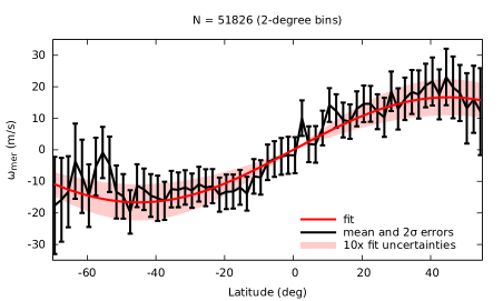
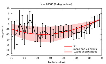
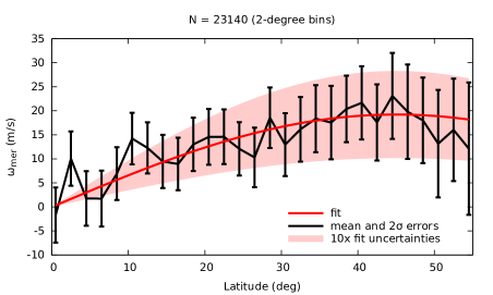
The small change in average closeness threshold does not significantly change the best fit parameters, and the values for D in both cases agree within $\pm 1\sigma_{D}$.

I calculate $\chi^{2}$ for these fits as

$$\chi^{2}=\sum_{i=1}^{N}\frac{(\omega_{mer,i}-\hat{\omega}_{mer,i})^{2}}{\sigma_{\mu,i}^{2}},$$ (7)

where the index $i$ runs over the $N$ latitudinal bins, $\omega_{mer,i}$ is the mean meridional speed in that bin, $\sigma_{\mu,i}$ is the standard error in the mean, and $\hat{\omega}_{mer,i}$ is the fit value using equation (5) and Table 4. Given only one free parameter, I estimate the number of degrees of freedom $\nu$ as $\nu=N-1$. For the fit to the measurement in both hemispheres with average closeness $\leq 1$, $D=16.66\text{ m s}^{-1}$ and thus $\chi^{2}=91.8$ and $\chi^{2}/\nu=1.48$. For a choice of significance level $\alpha=0.05$, the critical value of $\chi^{2}$ is $\sim 80$, so at the 95% level I must reject equation (5) as a good fit. However, I note that an outsize contribution of 13.2 to $\chi^{2}$ comes from a single latitudinal bin (-55°), and were I to remove this point as an outlier I would not reject equation (5) as a good fit. (This bin is too far south to be an artifact of active region inflow.) Instead of torturing the data further on this point, I simply assert that in order to assess the ability of equation (5) to describe my measurements, more analysis at higher latitudes is necessary to both reduce the measured uncertainties and to further constrain the trend of the mean at these latitudes.

4 Conclusions

In this paper, I describe the measurement of two long-lived photospheric flows, namely the differential rotation and meridional circulation, in a month-long dataset. The measurements were produced directly from the motions of both large- and small-scale individual magnetic features measured in high-cadence (12 min) magnetograms, rather than by correlating thin longitudinal strips or square patches over long time intervals. The high areal density of photospheric features and the length of the dataset results in $7.85\times 10^{6}$ tracked features. By selecting only long-lived, relatively isolated features, I am able to markedly reduce the effects of short-lived flows and apparent motion due to feature interactions. Because of the large number of features in the unfiltered dataset, this filtering still allows me to retain excellent statistical power in the differential rotation measurements and good power in the meridional flow measurements.

The style of my measurements is similar to the coronal bright point rotational measurements of Sudar et al. (2015), from which this work has benefited greatly. Coronal bright points have the advantage of being relatively sparse on the solar disk, and so are largely not subject to the same feature-interaction effects as photospheric magnetic features. I have successfully controlled for these in the case of differential rotation, and my results are largely consistent with past measurements. I find a rotational profile of $(14.296\pm 0.006)+(-1.847\pm 0.056)\sin^{2}b+(-2.615\pm 0.093)\sin^{4}b$, with units of $\textrm{ deg d}^{-1}$ and with covariances as given in Table 3, most importantly $\sigma_{BC}^{2}=-4.87\times 10^{-3}(\textrm{ deg d}^{-1})^{2}$. I note that to fully characterize the rotational profile using equation (3), future workers must specify the full covariance matrix of the parameters $A,B,C$, as in Table 3. Because the functions in equation (3) are not orthogonal, the variance in the quantities B & C over-estimates their uncertainties if the covariance $\sigma_{BC}^{2}$ is not reported. The covariance between the other pairs of parameters is relatively insignificant in this work.

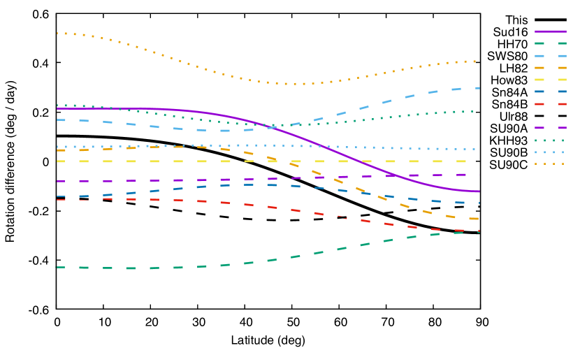
The solar surface rotation has been observed for hundreds of years, and with relatively high precision for the last 50 years. Beck (2000) provides a summary of results through the end of the 20th century, and Table 2 of Sudar et al. (2015) includes a few more recent results, including some coronal bright point measurements. I note that their coronal bright point measurements show $14.39\leq A\leq 14.65$, which is consistently faster than my measured $A=14.30$. Figure 6 compares the differential rotation curves from this work with the larger coronal bright point dataset of Sudar et al. (2016) as well as several spectroscopic and tracer references drawn from Beck (2000). Again, it is obvious that the rotation rate derived in this work is slower than that of the coronal bright point measurement. Considering that coronal bright points are believed to be anchored to small photospheric magnetic features, that most of the magnetic features used in the present work are small, and that the coronal bright points are consistently measured to rotate faster at the equator than the magnetic features, further work needs to be done to resolve this discrepancy. In comparison to previous surface measurements, the equatorial rotation rate found here is slower than two of the three tracer measurements (and slower than the third for latitudes poleward of 30°). Similarly, the equatorial rotation rate found here is faster than seven of the eight spectroscopic rotation rates; this trend is in agreement with previous assessments of the discrepancies between different measurement. I note that if my measured rotation curve were to hold all the way to the poles (where I did not in fact measure it), it would be the slowest there among all the results in Figure 6.

Figure 6: Comparison of differential rotation curves obtained from some published rotation coefficients, in which an arbitrarily-chosen background rotation curve (Howard et al., 1983) has been subtracted to emphasize the differences. Errors from uncertainties in the coefficients have been neglected for clarity. The rotation curve found in this work (solid black line) is consistently slower than the coronal bright point curve of Sudar et al. (2016) (solid purple line). Surface spectroscopic observations (dashed lines) and surface tracer observations (dotted lines) drawn from Beck (2000) are also plotted. HH70: Howard & Harvey (1970); SWS80: Scherrer et al. (1980); LH82: Labonte & Howard (1982); How83: (Howard et al., 1983); Sn84: Snodgrass (1984)(A - using all their data, B - using only their “best” data); Ulr88: Ulrich et al. (1988); SU90: Snodgrass & Ulrich (1990)(A - spectroscopic; B - correlation of daily magnetograms; C - correlation of supergranules in dopplergrams); KHH93: Komm et al. (1993).

My measurement of the meridional flow is noisier than that of the differential rotation, as expected. However, I do in all cases observe poleward motion in both hemispheres, the amplitude of which increases at least to latitudes of 45°. This is remarkable because at the 12 min cadence of my observations, and assuming a $15\text{ m s}^{-1}$ flow at 45°latitude, a feature would move 0.02 native HMI pixels (0.08 pixels in my reduced-scale images) per frame. My current observations are nearly fit well by equation (5) with a peak amplitude of $16.7\pm 0.6\text{ m s}^{-1}$, though more measurements are required to constrain the high-latitude behavior. That the measured flow speed increases to at least latitudes of 45°places this measurement in rough agreement with other measurements of meridional flow derived from magnetic tracking (e.g., Komm et al., 1993; Hathaway & Rightmire, 2010) and by extension also the coronal bright point results (Sudar et al., 2016), though I note that the peak flow amplitudes from the coronal bright points are $\sim$50% higher than reported here. These high latitude peak flows are in contrast with some measurements of the meridional flow from doppler shift, which show peak flows at lower latitudes (e.g., Ulrich, 2010). Dikpati et al. (2010) attribute the differences in these types of measurements to the effects of surface turbulent magnetic diffusion. I note that all measurements of meridional circulation on the surface and in the solar interior (e.g., Basu & Antia, 2010) show, over the course of the solar cycle, significant variations in the latitude and amplitude of the peak flow. For example, the Mount Wilson doppler-shift measurements show sharp low-latitude ($\sim$20°) peaks in the ascending phase of the solar cycle (1987–1990, 1997–2000) and broader mid-latitude ($\sim$40°) peaks during the declining phases (1992–1996, 2003–2008). Because the descending phase of the solar cycle is longer than the ascending phase, cycle averages tend to wash out the ascending phase peaks and result in broader peak flows than actually exist at a given time (Ulrich, 2010, Figures 6 and 7). Thus rigorous comparisons between measurements must take into account not only differences in the methods, but also the averaging done for each and their relative phase in the solar cycle.

This work shows that measuring the motions of individual features in photospheric magnetograms can produce high precision results in relatively short time spans. The relative ease by which this process could be automated suggests that higher resolution non-longitudinally averaged photospheric velocity residual measurements could be produced to compare with coronal results, and to provide other diagnostics of the solar dynamo.

References

- Babcock (1961) Babcock, H. W. 1961, ApJ, 133, 572
- Basu & Antia (2010) Basu, S., & Antia, H. M. 2010, ApJ, 717, 488
- Beck (2000) Beck, J. G. 2000, Sol. Phys., 191, 47
- Bevington & Robinson (2003) Bevington, P. R., & Robinson, D. K. 2003, Data reduction and error analysis for the physical sciences
- Charbonneau (2010) Charbonneau, P. 2010, Living Reviews in Solar Physics, 7, doi:10.12942/lrsp-2010-3
- Choudhuri (2015) Choudhuri, A. R. 2015, Journal of Astrophysics and Astronomy, 36, 5
- Cox (2000) Cox, A. N. 2000, Allen’s astrophysical quantities
- DeForest (2004) DeForest, C. E. 2004, Sol. Phys., 219, 3
- DeForest et al. (2007) DeForest, C. E., Hagenaar, H. J., Lamb, D. A., Parnell, C. E., & Welsch, B. T. 2007, ApJ, 666, 576
- Dikpati et al. (2010) Dikpati, M., Gilman, P. A., & Ulrich, R. K. 2010, ApJ, 722, 774
- Gilman & Howard (1984) Gilman, P. A., & Howard, R. 1984, ApJ, 283, 385
- Hagenaar (2001) Hagenaar, H. J. 2001, ApJ, 555, 448
- Hagenaar et al. (1999) Hagenaar, H. J., Schrijver, C. J., Title, A. M., & Shine, R. A. 1999, ApJ, 511, 932
- Hathaway & Rightmire (2010) Hathaway, D. H., & Rightmire, L. 2010, Science, 327, 1350
- Howard et al. (1983) Howard, R., Adkins, J. M., Boyden, J. E., et al. 1983, Sol. Phys., 83, 321
- Howard & Harvey (1970) Howard, R., & Harvey, J. 1970, Sol. Phys., 12, 23
- Howard & Labonte (1980) Howard, R., & Labonte, B. J. 1980, ApJ, 239, L33
- Howard et al. (1990) Howard, R. F., Harvey, J. W., & Forgach, S. 1990, Sol. Phys., 130, 295
- Komm et al. (2015) Komm, R., González Hernández, I., Howe, R., & Hill, F. 2015, Sol. Phys., 290, 3113
- Komm et al. (1993) Komm, R. W., Howard, R. F., & Harvey, J. W. 1993, Sol. Phys., 145, 1
- Labonte & Howard (1982) Labonte, B. J., & Howard, R. 1982, Sol. Phys., 80, 361
- Lamb et al. (2013) Lamb, D. A., Howard, T. A., DeForest, C. E., Parnell, C. E., & Welsch, B. T. 2013, ApJ, 774, 127
- Leighton (1964) Leighton, R. B. 1964, ApJ, 140, 1547
- Leighton (1969) —. 1969, ApJ, 156, 1
- Leka et al. (2013) Leka, K. D., Barnes, G., Birch, A. C., et al. 2013, ApJ, 762, 130
- Miesch et al. (2008) Miesch, M. S., Brun, A. S., DeRosa, M. L., & Toomre, J. 2008, ApJ, 673, 557
- Pesnell et al. (2012) Pesnell, W. D., Thompson, B. J., & Chamberlin, P. C. 2012, Sol. Phys., 275, 3
- Rajaguru & Antia (2015) Rajaguru, S. P., & Antia, H. M. 2015, ApJ, 813, 114
- Rightmire-Upton et al. (2012) Rightmire-Upton, L., Hathaway, D. H., & Kosak, K. 2012, ApJ, 761, L14
- Roša et al. (1995) Roša, D., Brajša, R., Vršnak, B., & Wöhl, H. 1995, Sol. Phys., 159, 393
- Scherrer et al. (1980) Scherrer, P. H., Wilcox, J. M., & Svalgaard, L. 1980, ApJ, 241, 811
- Scherrer et al. (2012) Scherrer, P. H., Schou, J., Bush, R. I., et al. 2012, Sol. Phys., 275, 207
- Sheeley (2005) Sheeley, Jr., N. R. 2005, Living Reviews in Solar Physics, 2, 5
- Skokić et al. (2014) Skokić, I., Brajša, R., Roša, D., Hržina, D., & Wöhl, H. 2014, Sol. Phys., 289, 1471
- Snodgrass (1984) Snodgrass, H. B. 1984, Sol. Phys., 94, 13
- Snodgrass & Ulrich (1990) Snodgrass, H. B., & Ulrich, R. K. 1990, ApJ, 351, 309
- Sudar et al. (2016) Sudar, D., Saar, S. H., Skokić, I., Poljančić Beljan, I., & Brajša, R. 2016, A&A, 587, A29
- Sudar et al. (2015) Sudar, D., Skokić, I., Brajša, R., & Saar, S. H. 2015, A&A, 575, A63
- Thompson et al. (1996) Thompson, M. J., Toomre, J., Anderson, E. R., et al. 1996, Science, 272, 1300
- Ulrich (2010) Ulrich, R. K. 2010, ApJ, 725, 658
- Ulrich et al. (1988) Ulrich, R. K., Boyden, J. E., Webster, L., Padilla, S. P., & Snodgrass, H. B. 1988, Sol. Phys., 117, 291
- Yeates et al. (2007) Yeates, A. R., Mackay, D. H., & van Ballegooijen, A. A. 2007, Sol. Phys., 245, 87
- Zhao et al. (2013) Zhao, J., Bogart, R. S., Kosovichev, A. G., Duvall, Jr., T. L., & Hartlep, T. 2013, ApJ, 774, L29