Chapter 0 Orthogonal polynomials of several variables

Yuan Xu

1 Introduction

Polynomials of $d$ variables are indexed by the set ${\mathbb{N}}_{0}^{d}$ of multi-indices, where ${\mathbb{N}}_{0}:=\{0,1,2,\ldots\}$. The standard multi-index notations will be used throughout this chapter. For $\alpha=(\alpha_{1},\ldots,\alpha_{d})\in{\mathbb{N}}_{0}^{d}$ and $x=(x_{1},\ldots,x_{d})$, a monomial $x^{\alpha}$ is defined by $x^{\alpha}=x_{1}^{\alpha_{1}}\ldots x_{d}^{\alpha_{d}}$. The number $|\alpha|=\alpha_{1}+\cdots+\alpha_{d}$ is called the (total) degree of $x^{\alpha}$. The space of homogeneous polynomials of degree $n$ is denoted by

$${\mathcal{P}}_{n}^{d}:=\textrm{span}\left\{x^{\alpha}\;\big{|}\;|\alpha|=n,\;\alpha\in{\mathbb{N}}_{0}^{d}\right\}$$

and the space of polynomials of degree at most $n$ is denoted by

$$\Pi_{n}^{d}:=\textrm{span}\left\{x^{\alpha}\;\big{|}\;|\alpha|\leq n,\;\alpha\in{\mathbb{N}}_{0}^{d}\right\}.$$

Evidently, $\Pi_{n}^{d}$ is a direct sum of ${\mathcal{P}}_{k}^{d}$ for $k=0,1,\ldots,n$. Furthermore,

$$\dim{\mathcal{P}}_{n}^{d}=\binom{n+d-1}{n}\quad\hbox{and}\quad\dim\Pi_{n}^{d}=\binom{n+d}{n}.$$ (1)

Let ${\langle}\cdot,\cdot{\rangle}$ be an inner product defined on the space of polynomials of $d$ variables. A priori it may be indefinite or even degenerate. Usually it will be given by

$${\langle}f,g{\rangle}_{\mu}:=\int_{{\mathbb{R}}^{d}}f(x)g(x)\,d\mu(x),$$

where the orthogonality measure $\mu$ is a positive Borel measure on ${\mathbb{R}}^{d}$ such that the integral is well defined on polynomials. This inner product will be nondegenerate, and hence positive definite if $\mu$ is supported on a set $\Omega$ that has nonempty interior. This will almost always be the case in this chapter, apart from some exceptional cases in §8.

A polynomial $P\in\Pi_{n}^{d}$ is said to be an orthogonal polynomial of degree $n$ with respect to ${\langle}\cdot,\cdot{\rangle}$ if $P$ is orthogonal to all polynomials of degree $<n$:

$${\langle}P,Q{\rangle}=0,\qquad\forall Q\in\Pi^{d}\quad\hbox{with}\quad\deg Q<\deg P.$$ (2)

However, two linearly independent orthogonal polynomials of degree $n$ are not necessarily orthogonl to each other. Let ${\mathcal{V}}_{n}^{d}$ be the space of orthogonal polynomials of degree $n$, that is,

$${\mathcal{V}}_{n}^{d}:=\left\{P\in\Pi_{n}^{d}\;\big{|}\;{\langle}P,Q{\rangle}=0,\quad\forall Q\in\Pi_{n-1}^{d}\right\}.$$ (3)

If the inner product is nondegenerate then $\dim{\mathcal{V}}_{n}^{d}=\dim{\mathcal{P}}_{n}^{d}=\binom{n+d-1}{n}:=r_{n}^{d}$, and $\Pi_{n}^{d}$ is a direct sum of ${\mathcal{V}}_{k}^{d}$ for $k=0,1,\ldots,n$.

Given a nondegenerate inner product, we can assign to the set $\big{\{}x^{\alpha}\mid\alpha\in{\mathbb{N}}_{0}^{d}\big{\}}$ a linear order $\succ$ which is graded (i.e., $x^{\alpha}\succ x^{\beta}$ if $|\alpha|>|\beta|$), and apply the Gram–Schmidt orthogonalization process to generate a sequence of orthogonal polynomials. In contrast to $d=1$, however, there is no obvious natural graded order among monomials when $d>1$. There are instead many well defined orders. One example is given by the graded lexicographic order:
$x^{\alpha}\succ x^{\beta}$ if $|\alpha|>|\beta|$ or if $|\alpha|=|\beta|$ and the first nonzero entry in the difference $\alpha-\beta$ is positive.
In general, different orderings will lead to different orthogonal systems. Consequently, orthogonal polynomials of several variables are not unique. Moreover, any system of orthogonal polynomials obtained by an ordering of the monomials is necessarily unsymmetric in the variables $x_{1},\ldots,x_{d}$. These were recognized as the essential difficulties in the study of orthogonal polynomials of several variables in [33, Ch. XII], which contains a rather comprehensive account of the results up to 1950.

A sequence of polynomials $\{P_{\alpha}\}\in{\mathcal{V}}_{n}^{d}$ is called orthogonal if ${\langle}P_{\alpha},P_{\beta}{\rangle}=0$ whenever ${\alpha}\neq{\beta}$, and orthonormal if moreover ${\langle}P_{\alpha},P_{\alpha}{\rangle}=1$ for all ${\alpha}$. The space ${\mathcal{V}}_{n}^{d}$ can have many different bases and a basis does not have to be orthogonal. One way to extend the theory of orthogonal polynomials of one variable to several variables is to state the results in terms of ${\mathcal{V}}^{d}_{0},{\mathcal{V}}^{d}_{1},\ldots,{\mathcal{V}}^{d}_{n},\ldots$, rather than in terms of a particular basis in each ${\mathcal{V}}^{d}_{n}$.

This point of view will be prominent in our next section, which contains a brief account on the general properties of the orthogonal polynomials of several variables, mostly developed in the last two decades. In the later sections of this chapter, we will discuss in more details specific systems of orthogonal polynomials in two and more variables that correspond to, or are generalizations of, the classical orthogonal polynomials of one variable. Most of these systems are of separated type, by which we mean that a basis of orthogonal polynomials can be expressed as products in some separation of variables in terms of classical orthogonal polynomials of one variable.

There are many points of contact with other chapters of this volume. Some of the orthogonal polynomials will be given in terms of Appell and Lauricella hypergeometric functions, which are the subject of Chapter 3. Orthogonal polynomials for weight function invariant under a reflection group are addressed in Chapter 7. Orthogonal polynomials associated with root systems are treated in Chapter 8. $q$-Analogues of such orthogonal polynomials are discussed in Chapter 9.

2 General properties of orthogonal polynomials of several variables

The general properties of orthogonal polynomials of several variables were studied as early as as 1936 by Jackson [57]. Most earlier studies dealt with two variables, see references in [33, Ch. XII] and [103]. The presentation below follows the book [28] by Dunkl and Xu.

1 Moments and orthogonal polynomials

Associated with each multi-sequence $s\colon{\mathbb{N}}_{0}^{d}\mapsto{\mathbb{R}}$, $s=(s_{\alpha})_{{\alpha}\in{\mathbb{N}}_{0}^{d}}$, we can define a linear functional ${\mathcal{L}}$, called moment functional, by

$${\mathcal{L}}(x^{\alpha})=s_{\alpha},\qquad{\alpha}\in{\mathbb{N}}_{0}^{d}.$$

A polynomial $P\in\Pi_{n}^{d}$ is called orthogonal with respect to ${\mathcal{L}}$ if it is orthogonal with respect to the bilinear form ${\langle}f,g{\rangle}={\mathcal{L}}(fg)$, which however is not necessarily a positive definite or nondegenerate inner product.

For each $n\in{\mathbb{N}}_{0}$ let ${\mathbf{x}}^{n}$ denote the column vector

$${\mathbf{x}}^{n}:=(x^{\alpha})_{|\alpha|=n}=(x^{\alpha_{j}})_{j=1}^{r_{n}^{d}},$$

where $\alpha_{1},\alpha_{2},\ldots,\alpha_{r_{n}^{d}}$, $r_{n}^{d}=\dim{\mathcal{P}}_{n}^{d}$, is the arrangement of the elements in $\big{\{}\alpha\in{\mathbb{N}}_{0}^{d}\mid|\alpha|=n\big{\}}$ according to the lexicographical order. For $k,j\in{\mathbb{N}}_{0}$ define a vector of moments ${\mathbf{s}}_{k}$ and a matrix of moments ${\mathbf{s}}_{k,j}$ by

$${\mathbf{s}}_{k}:={\mathcal{L}}({\mathbf{x}}^{k})\quad\hbox{and}\quad{\mathbf{s}}_{k,j}={\mathbf{s}}_{\{k\}+\{j\}}:={\mathcal{L}}({\mathbf{x}}^{k}({\mathbf{x}}^{j})^{\mathsf{tr}}).$$ (4)

By definition, ${\mathbf{s}}_{\{k\}+\{j\}}$ is a matrix of size $r_{k}^{d}\times r_{j}^{d}$, its elements are $s_{\alpha+\beta}$ for $|\alpha|=k$ and $|\beta|=j$. Finally, for each $n\in{\mathbb{N}}_{0}$, we define a moment matrix by using ${\mathbf{s}}_{\{k\}+\{j\}}$ as its building blocks,

$$M_{n,d}:=\left({\mathbf{s}}_{\{k\}+\{j\}}\right)_{k,j=0}^{n}\quad\hbox{and}\quad\Delta_{n,d}:=\det M_{n,d}.$$ (5)

The elements of $M_{n,d}$ are $s_{{\alpha}+{\beta}}$ for $|\alpha|\leq n$ and $|\beta|\leq n$.

Theorem 2.1.

[28, Theorem 3.2.6]
Let ${\mathcal{L}}$ be a moment functional. The corresponing inner product is nondegenerate

if and only if $\Delta_{n,d}\neq 0$ for all $n\in{\mathbb{N}}_{0}$.

From now on in this section we assume the above nondegeneracy condition. Then orthogonal bases of ${\mathcal{V}}_{n}^{d}$ esist. A special, usually not orthogonal, basis can be expressed in terms of moments ${\mathcal{L}}$ as follows. For ${\alpha}\in{\mathbb{N}}_{0}^{d}$ we denote by ${\mathbf{s}}_{{\alpha},k}$ the column vector ${\mathbf{s}}_{{\alpha},k}:={\mathcal{L}}(x^{\alpha}{\mathbf{x}}^{k})$; in particular, ${\mathbf{s}}_{{\alpha},0}=s_{\alpha}$.

Theorem 2.2.

[28, Theorem 3.2.12]
For $|{\alpha}|=n$, the polynomials

$$P_{\alpha}^{n}(x):=\frac{1}{\Delta_{n-1,d}}\det\left[\begin{array}[]{c|c}M_{n-1,d}&\begin{matrix}{\mathbf{s}}_{{\alpha},0}\\ {\mathbf{s}}_{{\alpha},1}\\ \vdots\\ {\mathbf{s}}_{{\alpha},n-1}\end{matrix}\\ \hline\cr 1,{\mathbf{x}}^{\mathsf{tr}}\ldots({\mathbf{x}}^{n-1})^{\mathsf{tr}}&x^{\alpha}\end{array}\right]$$ (6)

form a basis for the space ${\mathcal{V}}_{n}^{d}$ of orthogonal polynomials of degree $n$ with respect to ${\mathcal{L}}$.

The polynomial $P_{\alpha}^{n}$ can also be characterized as the unique polynomial in ${\mathcal{V}}_{n}^{d}$ of the form

$$P_{\alpha}^{n}(x)=x^{\alpha}+Q_{n-1}(x),\qquad Q_{n-1}\in\Pi_{n-1}^{d}.$$

It is evident that a polynomial thus characterized exists. Because of the leading term $x^{\alpha}$ the basis $\{P_{\alpha}^{n}\}_{|{\alpha}|=n}$ is called a monic or monomial basis of orthogonal polynomials.

If ${\mathcal{L}}(p^{2})>0$ for all nonzero polynomials $p$, then the moment functional ${\mathcal{L}}$ is called positive definite. In that case the corresponding inner product ${\langle}f,g{\rangle}={\mathcal{L}}(fg)$ is also positive definite and orthonormal bases of polynomials with respect to ${\mathcal{L}}$ will exist.

Theorem 2.3.

[28, Lemma 3.2.8] If ${\mathcal{L}}$ is positive definite, then $\Delta_{n,d}>0$ for all $n\in{\mathbb{N}}_{0}$.

For a sequence of polynomials $\big{\{}P_{\alpha}\mid|{\alpha}|=n\big{\}}$, we denote by ${\mathbb{P}}_{n}$ the polynomial (column) vector

$${\mathbb{P}}_{n}:=(P_{\alpha}^{n})_{|\alpha|=n}=(P_{\alpha^{(1)}}^{n},\ldots,P_{\alpha^{(r_{n})}}^{n})^{\mathsf{tr}},$$ (7)

where $\alpha^{(1)},\ldots,\alpha^{(r_{n})}$ is the arrangement of elements in $\{\alpha\in{\mathbb{N}}_{0}^{d}:|\alpha|=n\}$ according to a fixed monomial order. We also regard ${\mathbb{P}}_{n}$ as a set of polynomials $\big{\{}P_{\alpha}^{n}\mid|{\alpha}|=n\big{\}}$. Many properties of orthogonal polynomials of several variables can be expressed more compactly in terms of ${\mathbb{P}}_{n}$. For example, orthonormality of $\big{\{}P_{\alpha}\mid{\alpha}\in{\mathbb{N}}_{0}^{d}\big{\}}$ with respect to ${\langle}\cdot,\cdot{\rangle}$ can be written as

$${\langle}{\mathbb{P}}_{n},{\mathbb{P}}_{m}{\rangle}=\delta_{m,n}I_{r_{n}^{d}},$$

where $I_{k}$ denote the identity matrix of size $k\times k$.

The rows of $M_{n,d}$ are indexed by $\{{\alpha}:|{\alpha}|\leq n\}$. The row indexed by ${\alpha}$ is

$$({\mathbf{s}}_{{\alpha},0}^{\mathsf{tr}},{\mathbf{s}}_{\alpha,1}^{\mathsf{tr}},\ldots,{\mathbf{s}}_{\alpha,n}^{\mathsf{tr}})={\mathcal{L}}\left(x^{\alpha},x^{\alpha}{\mathbf{x}}^{\mathsf{tr}},\ldots,x^{\alpha}({\mathbf{x}}^{n})^{\mathsf{tr}}\right).$$

For $|{\alpha}|=n$, let $\widetilde{M}_{{\alpha}}(x)$ be the matrix obtained from $M_{n,d}$ by replacing the above row of index ${\alpha}$ by $\left(1,{\mathbf{x}}^{\mathsf{tr}},\ldots,({\mathbf{x}}^{n})^{\mathsf{tr}}\right).$ Define

$$\widetilde{P}_{\alpha}(x):=\frac{1}{\Delta_{n,d}}\det\widetilde{M}_{\alpha}(x),\qquad|{\alpha}|=n,\quad{\alpha}\in{\mathbb{N}}_{0}^{d}.$$

Let $N_{n,d}$ denote the principal submatrix of the inverse matrix $M_{n,d}^{-1}$ of size $r_{n}^{d}\times r_{n}^{d}$ at the lower right corner. Then $N_{n,d}$ is positive definite.

Theorem 2.4.

[28, Theorem 3.2.13, (3.2.14)]
Let ${\mathcal{L}}$ be a positive definite moment functional. Then

$${\mathbb{P}}_{n}(x):=(N_{n,d})^{-\frac{1}{2}}\widetilde{\mathbb{P}}_{n}(x)=G_{n}{\mathbf{x}}^{n}+\cdots$$ (8)

consists of orthonormal polynomials. Furthermore, the matrix $G_{n}$ is positive definite and

$$G_{n}=(N_{n,d})^{\frac{1}{2}},\qquad\det G_{n}=(\Delta_{n-1,d}/\Delta_{n,d})^{1/2}.$$

As mentioned before, the space of orthogonal polynomials ${\mathcal{V}}_{n}^{d}$ of degree $n$ has many different bases. The orthonormal bases, however, are unique up to orthogonal transformations.

Theorem 2.5.

[28, Theorem 3.2.14]
Let ${\mathcal{L}}$ be positive definite and let $\{Q_{\alpha}^{n}\}$ be a sequence of orthonormal polynomials forming a basis of ${\mathcal{V}}_{n}^{d}$. Then there is an orthogonal matrix $O_{n}$ such that ${\mathbb{Q}}_{n}=O_{n}{\mathbb{P}}_{n}$, where ${\mathbb{P}}_{n}$ are the orthonormal polynomials defined in (8).

Let ${\mathcal{M}}={\mathcal{M}}({\mathbb{R}}^{d})$ denote the set of nonnegative Borel measures on ${\mathbb{R}}^{d}$ such that $\int_{{\mathbb{R}}^{d}}|x^{\alpha}|d\mu(x)<\infty$ for all ${\alpha}\in{\mathbb{N}}_{0}^{d}$. Each $\mu\in{\mathcal{M}}$ defines a positive linear functional

$${\mathcal{L}}f=\int_{{\mathbb{R}}^{d}}f(x)\,d\mu(x),\qquad f\in\Pi^{d}.$$ (9)

A polynomial $p$ is orthogonal with respect to the orthogonality measure $\mu$ if it is orthogonal with respect to ${\mathcal{L}}$ defined in (9). Thus, all theorems in this subsection apply to the orthogonal polynomials with respect to $d\mu$ for $\mu\in{\mathcal{M}}$.

On the other hand, not every positive definite linear functional admits an integral representation (9). The moment problem asks when a linear functional, defined via its moments, admits an integral representation (9) for a $\mu\in{\mathcal{M}}$ and, if so, when the measure will be determinate. Here a measure $\mu$ is called determinate if no other measure in ${\mathcal{M}}$ has all its moments equal to those of $\mu$. It is known that ${\mathcal{L}}$ admits an integral representation if, and only if, ${\mathcal{L}}$ is positive in the sense that ${\mathcal{L}}p\geq 0$ for every nonnegative polynomial $p$. Evidently a positive linear functional is necessarily positive semidefinite (i.e, ${\mathcal{L}}p^{2}\geq 0$ for every polynomial $p$), which also holds sufficiently for $d=1$. For $d>1$, however, a positive definite linear functional may not be positive: there existnonnegative polynomials that cannot be written as a sum of squared polynomials. For moment problems of several variables, including various sufficient conditions on a measure being determinate, see [13, 38, 97] and references therein.

2 Three-term relations

Every system of orthogonal polynomials of one variable satisfies a three term relation, which can also be used to compute orthogonal polynomials recursively. For orthogonal polynomials of several variables, an analogue of the three-term relation is stated in terms of ${\mathcal{V}}_{n}^{d}$, or rather, in terms of ${\mathbb{P}}_{n}$.

Theorem 2.6.

[28, Theorem 3.3.1]
Let ${\mathbb{P}}_{n}$ denote a basis of ${\mathcal{V}}_{n}^{d}$, $n=0,1,\ldots$ and let ${\mathbb{P}}_{-1}(x):=0$. Then there exist unique matrices $A_{n,i}\colon r_{n}^{d}\times r^{d}_{n+1}$, $B_{n,i}\colon r_{n}^{d}\times r_{n}^{d}$, and $C_{n,i}\colon r_{n}^{d}\times r^{d}_{n-1}$ for $n=0,1,2,\ldots$, such that

$$x_{i}{\mathbb{P}}_{n}(x)=A_{n,i}{\mathbb{P}}_{n+1}(x)+B_{n,i}{\mathbb{P}}_{n}(x)+C_{n,i}{\mathbb{P}}_{n-1}(x),\quad 1\leq i\leq d.$$ (10)

In fact, let $H_{n}:={\mathcal{L}}({\mathbb{P}}_{n}{\mathbb{P}}_{n}^{\mathsf{tr}})$; then the orthogonality shows that

$$A_{n,i}H_{n+1}={\mathcal{L}}(x_{i}{\mathbb{P}}_{n}{\mathbb{P}}_{n+1}^{\mathsf{tr}}),\quad B_{n,i}H_{n}={\mathcal{L}}(x_{i}{\mathbb{P}}_{n}{\mathbb{P}}_{n}^{\mathsf{tr}}),\quad A_{n,i}H_{n+1}=H_{n}C_{n+1,i}^{\mathsf{tr}}.$$

The coefficient matrices $A_{n,i}$ and $C_{n,i}$ in (10) have full rank. Indeed,

$$\operatorname{rank}A_{n,i} =\operatorname{rank}C_{n+1,i}=r_{n}^{d},$$ (11)

$$\operatorname{rank}A_{n} =\operatorname{rank}C_{n+1}^{\mathsf{tr}}=r_{n+1}^{d},$$ (12)

where $A_{n}=(A_{n,1}^{\mathsf{tr}},\ldots,A_{n,d}^{\mathsf{tr}})^{\mathsf{tr}}$ and $C_{n+1}^{\mathsf{tr}}=(C_{n+1,1},\ldots,C_{n+1,d})^{\mathsf{tr}}$ are matrices of size $dr_{n}^{d}\times r_{n+1}^{d}$. In the case of orthonormal polynomials, $H_{n}$ is the identity matrix and the three-term relation takes a simpler form.

Theorem 2.7.

[28, Theorem 3.3.2]
If ${\mathbb{P}}_{n}$ is an orthonormal basis of ${\mathcal{V}}_{n}^{d}$, $n=0,1,\ldots$, then

$$x_{i}{\mathbb{P}}_{n}(x)=A_{n,i}{\mathbb{P}}_{n+1}(x)+B_{n,i}{\mathbb{P}}_{n}(x)+A_{n-1,i}^{\mathsf{tr}}{\mathbb{P}}_{n-1}(x),\quad 1\leq i\leq d,$$ (13)

where $A_{n,i}={\mathcal{L}}(x_{i}{\mathbb{P}}_{n}{\mathbb{P}}_{n+1}^{\mathsf{tr}})$, $B_{n,i}={\mathcal{L}}(x_{i}{\mathbb{P}}_{n}{\mathbb{P}}_{n}^{\mathsf{tr}})$ and $B_{n,i}$ is symmetric.

As an analogue of the classical Favard’s theorem for orthogonal polynomials of one variable, the three-term relation and the rank conditions characterize orthogonality.

Theorem 2.8.

[28, Theorem 3.3.8]
Let $\{{\mathbb{P}}_{n}\}_{n=0}^{\infty}=\big{\{}P_{\alpha}^{n}\mid|\alpha|=n,n\in{\mathbb{N}}_{0}\big{\}}$, ${\mathbb{P}}_{0}=1$, be an arbitrary sequence in $\Pi^{d}$ such that $\big{\{}P_{\alpha}^{m}\mid|{\alpha}|=m\leq n\big{\}}$ spans $\Pi_{n}^{d}$ for each $n$. Then the following statements are equivalent.

1. There exists a positive definite linear functional ${\mathcal{L}}$ that makes $\{{\mathbb{P}}_{n}\}_{n=0}^{\infty}$ an orthonormal basis for $\Pi^{d}$.

2. For $n\geq 0$, $1\leq i\leq d$, there exist matrices $A_{n,i}$ and $B_{n,i}$ such that

   1. $x_{i}{\mathbb{P}}_{n}(x)=A_{n,i}{\mathbb{P}}_{n+1}(x)+B_{n,i}{\mathbb{P}}_{n}(x)+A_{n-1,i}^{\mathsf{tr}}{\mathbb{P}}_{n-1}(x),\quad 1\leq i\leq d,$

   2. $\operatorname{rank}A_{n,i}=r_{n}^{d},\quad 1\leq i\leq d$, and $\operatorname{rank}A_{n}=r_{n+1}^{d}$.

Unlike in one variable, the characterization does not conclude about the existence of an orthogonality measure.

The coefficient matrices of the three-term relation for orthonormal polynomials satisfy a set of commutativity conditions [28, Theorem 3.4.1]: for $1\leq i,j\leq d$ and $k\geq 0$,

$$A_{k,i}A_{k+1,j} =A_{k,j}A_{k+1,i},$$

$$A_{k,i}B_{k+1,j}+B_{k,i}A_{k,j} =B_{k,j}A_{k,i}+A_{k,j}B_{k+1,i},$$ (14)

$$A_{k-1,i}^{\mathsf{tr}}A_{k-1,j}+B_{k,i}B_{k,j}+A_{k,i}A_{k,j}^{\mathsf{tr}} =A_{k-1,j}^{\mathsf{tr}}A_{k-1,i}+B_{k,i}B_{k,j}+A_{k,j}A_{k,i}^{\mathsf{tr}},$$

where $A_{-1,i}:=0$, which is derived from computing, say, ${\mathcal{L}}(x_{i}x_{j}{\mathbb{P}}_{k}{\mathbb{P}}_{k-1})$, by applying the three-term relation in two different ways. These coefficient matrices also define a family of tri-diagonal matrices $J_{i}$, $1\leq i\leq d$:

$$J_{i}=\left[\begin{matrix}B_{0,i}&A_{0,i}&&\bigcirc\cr A_{0,i}^{\mathsf{tr}}&B_{1,i}&A_{1,i}&&\cr&A_{1,i}^{\mathsf{tr}}&B_{2,i}&\ddots\cr\bigcirc&&\ddots&\ddots\end{matrix}\right],\qquad 1\leq i\leq d,$$ (15)

called block Jacobi matrices. The entries of the $J_{i}$ are matrices that have increasing sizes going down the main diagonal. The commutativity relations (2) is equivalent to the formal commutativity of $J_{i}$ [28, Lemma 3.4.4], that is,

$$J_{i}J_{j}=J_{j}J_{i},\qquad 1\leq i\neq j\leq d.$$

These block Jacobi matrices can be viewed as the realization of the multiplication operators $X_{1},\ldots,X_{d}$ defined on the space of polynomials by

$$(X_{i}f)(x)=x_{i}f(x),\qquad 1\leq i\leq d.$$

The operators can be extended to a family of commuting self-adjoint operators on a $L^{2}$ space. This connection to the operator theory allows the use of the spectral theory of commuting self-adjoint operators, and helps to answer the question when the inner product with respect to which polynomials are orthogonal is defined by a measure. It gives, for example, the following theorem, which strengthens Theorem 2.8:

Theorem 2.9.

[28, Theorem 3.4.7]
Let $\{{\mathbb{P}}_{n}\}_{n=0}^{\infty}=\big{\{}P_{\alpha}^{n}\mid|\alpha|=n,n\in{\mathbb{N}}_{0}\big{\}}$, ${\mathbb{P}}_{0}=1$, be an arbitrary sequence in $\Pi^{d}$ such that $\{P_{\alpha}^{m}\mid|{\alpha}|=m\leq n\}$ spans $\Pi_{n}^{d}$ for each $n$. Then the following statements are equivalent.

1. There exists a determinate measure $\mu\in{\mathcal{M}}$ with compact support in ${\mathbb{R}}^{d}$ such that $\{{\mathbb{P}}_{n}\}_{n=0}^{\infty}$ is orthonormal with respect to $d\mu$.

2. The statement (2) in Theorem 2.8 holds together with

   $$\sup_{k\geq 0}\|A_{k,i}\|_{2}<\infty\quad\hbox{and}\quad\sup_{k\geq 0}\|B_{k,i}\|_{2}<\infty,\quad 1\leq i\leq d.$$ (16)

If the measure $\mu\in{\mathcal{M}}$ is given by $d\mu(x)=W(x)\,dx$, $W$ being a nonnegative measurable function, we call $W$ a weight function, Let $\Omega\subset{\mathbb{R}}^{d}$ be the support set of $W$. A function $W$ is called centrally symmetric, if

$$x\in\Omega\Rightarrow-x\in\Omega,\quad\hbox{and}\quad W(x)=W(-x)\hbox{ a.e.\;.}$$

For example, the product weight function $\prod_{i=1}^{d}(1-x_{i})^{a_{i}}(1+x_{i})^{b_{i}}$ on the cube $[-1,1]^{d}$ is centrally symmetric if and only if $a_{i}=b_{i}$. Furthermore, a linear functional ${\mathcal{L}}$ is called centrally symmetric if

$${\mathcal{L}}(x^{\alpha})=0,\quad\alpha\in{\mathbb{N}}^{d},\quad|\alpha|\hbox{ is odd integer}.$$

The two notions are equivalent when ${\mathcal{L}}$ is given by ${\mathcal{L}}f=\int fW\,dx$.

Theorem 2.10.

[28, Theorem 3.3.10]
Let ${\mathcal{L}}$ be a positive definite linear functional. Then ${\mathcal{L}}$ is centrally symmetric if and only if $B_{n,i}=0$ for all $n\in{\mathbb{N}}_{0}$ and $1\leq i\leq d$, where $B_{n,i}$ are given in (13). Furthermore, if ${\mathcal{L}}$ is centrally symmetric, then an orthogonal polynomial of degree $n$ is a sum of monomials of even degrees if $n$ is even, and a sum of monomials of odd degrees if $n$ is odd.

In one variable, the three term relation can be used as a recurrence formula for computing orthogonal polynomials of one variable. For several variables, let $D_{n}^{\mathsf{tr}}=(D_{n,1}^{\mathsf{tr}},\ldots,D_{n,d}^{\mathsf{tr}})$, where $D_{n,i}^{\mathsf{tr}}\colon r^{d}_{n+1}\times r_{n}^{d}$, be a matrix that satisfies

$$D_{n}^{\mathsf{tr}}A_{n}=\sum_{i=1}^{d}D_{n,i}^{\mathsf{tr}}A_{n,i}=I_{r_{n+1}^{d}}.$$

Such a matrix is not unique. The three-term relation (13) implies

$${\mathbb{P}}_{n+1}=\sum_{i=1}^{d}x_{i}D^{\mathsf{tr}}_{n,i}{\mathbb{P}}_{n}+E_{n}{\mathbb{P}}_{n}+F_{n}{\mathbb{P}}_{n-1},$$ (17)

where $E_{n}:=-\sum_{i=1}^{d}D_{n,i}^{\mathsf{tr}}B_{n,i}$ and $F_{n}:=-\sum_{i=1}^{d}D_{n,i}^{\mathsf{tr}}A^{\mathsf{tr}}_{n-1,i}$.

Given two sequences of matrices $A_{n,i}$ and $B_{n,i}$, (17) can be used as a recursive relation to generate a sequence of polynomials. These polynomials are orthogonal if the matrices satisfy certain relations:

Theorem 2.11.

[28, Theorem 3.5.1]
Let $\{{\mathbb{P}}_{n}\}_{n=0}^{\infty}$ be defined by (17). Then there is a positive definite linear functional ${\mathcal{L}}$ that makes $\{{\mathbb{P}}_{n}\}_{n=0}^{\infty}$ an orthonormal basis for $\Pi^{d}$ if and only if $B_{k,i}$ are symmetric, $A_{k,i}$ satisfy the rank conditions (11) and (12), and together they satisfy the commutativity conditions (2).

Further results and references The idea of studying orthogonal polynomials of several variables in terms of ${\mathcal{V}}_{0}^{d},{\mathcal{V}}_{1}^{d},\,\ldots$  goes back to [67]. The vector notion of three-term relation and Favard’s theorem were initiated by M. Kowalski in [66, 65]. The versions in this section were developed by Xu in [115, 117] and subsequent papers. Another earlier work is [39]. See [28, Chapter 3] for references and further results.

For further study of three-term relations, see [16]. For an approach based on matrix factorization, see [6]. Three-term relations are used for evaluating orthogonal polynomials of several variables in [8].

3 Zeros of orthogonal polynomials of several variables

An orthogonal polynomial of degree $n$ in one variable has $n$ distinct real zeros and the zeros are nodes of a Gaussian quadrature formula. For a polynomial of several variables, its set of zero is an algebraic variety, an intrinsically difficult object. The correct notion for orthogonal polynomials of several variables are the common zeros of a family of polynomials, such as ${\mathbb{P}}_{n}$.

Let ${\mathbb{P}}_{n}$ be an orthonormal basis of ${\mathcal{V}}_{n}^{d}$. A point $x\in{\mathbb{R}}^{d}$ is a zero of ${\mathbb{P}}_{n}$ if it is a zero for every elements in ${\mathbb{P}}_{n}$ (or all elements in ${\mathcal{V}}_{n}^{d}$), and it is a simple zero if at least one partial derivative of ${\mathbb{P}}_{n}$ is not zero at $x$. Let $A_{n,i}$ and $B_{n,i}$ be matrices in (13). For each $n\in{\mathbb{N}}_{0}$, define the truncated block Jacobi matrices

$$J_{n,i}:=\left[\begin{matrix}B_{0,i}&A_{0,i}&&&\bigcirc\cr A_{0,i}^{\mathsf{tr}}&B_{1,i}&A_{1,i}&&\cr&\ddots&\ddots&\ddots&\cr&&A_{n-3,i}^{\mathsf{tr}}&B_{n-2,i}&A_{n-2,i}\cr\bigcirc&&&A_{n-2,i}^{\mathsf{tr}}&B_{n-1,i}\end{matrix}\right],\qquad 1\leq i\leq d.$$

These are symmetric matrices of order $N=\dim\Pi_{n-1}^{d}$. An element ${\lambda}\in{\mathbb{R}}^{d}$ is called a joint eigenvalue of $J_{n,1},\ldots,J_{n,d}$, if there is a $\xi\neq 0$, $\xi\in{\mathbb{R}}^{N}$, such that $J_{n,i}\xi={\lambda}_{i}\xi$ for $i=1,\ldots,d$; the vector $\xi$ is called a joint eigenvector.

Theorem 2.12.

[28, Theorem 3.7.2]
A point ${\lambda}\in{\mathbb{R}}^{d}$ is a common zero of ${\mathbb{P}}_{n}$ if and only if it is a joint eigenvalue of $J_{n,1},\ldots,J_{n,d}$; moreover, a joint eigenvector of ${\lambda}$ is $({\mathbb{P}}_{0}^{\mathsf{tr}}({\lambda}),\ldots,{\mathbb{P}}_{n-1}^{\mathsf{tr}}({\lambda}))^{\mathsf{tr}}$.

Many properties of zeros of ${\mathbb{P}}_{n}$ can be derived from this characterization.

Theorem 2.13.

[28, Theorem 3.7.1, 3.7.5, Corollary 3.7.3, 3.7.4]
All zeros of ${\mathbb{P}}_{n}$ are real, distinct and simple. ${\mathbb{P}}_{n}$ has at most $\dim\Pi_{n-1}^{d}$ distinct zeros, and ${\mathbb{P}}_{n}$ has $\dim\Pi_{n-1}^{d}$ zeros if and only if

$$A_{n-1,i}A_{n-1,j}^{\mathsf{tr}}=A_{n-1,j}A_{n-1,i}^{\mathsf{tr}},\quad 1\leq i,j\leq d.$$ (18)

Theorem 2.14.

[28, Corollary 3.7.7], [116, Theorem 3.1.1]
If $L$ is centrally symmetric and $d\geq 2$, then ${\mathbb{P}}_{n}$ has less than $\dim\Pi_{n-1}^{d}$ common zeros.
If moreover $d=2$, then ${\mathbb{P}}_{n}$ has no zero if $n$ is even and has one zero $(x=0)$ if $n$ is odd.

As in the case of one variable, zeros of orthogonal polynomials are closely related to cubature formulas, which are finite sums that approximate integrals. A cubature formula ${\mathcal{I}}_{\!n}(f)$ is said to have degree $2n-1$ if

$$\int_{{\mathbb{R}}^{d}}f(x)\,d\mu(x)=\sum_{k=1}^{N}{\lambda}_{k}f(x_{k})=:{\mathcal{I}}_{\!n}(f),\quad\forall f\in\Pi_{2n-1}^{d},$$ (19)

where ${\lambda}_{k}\in{\mathbb{R}}$ and $x_{k}\in{\mathbb{R}}^{d}$, and there is a polynomial $f^{*}\in\Pi_{2n}^{d}$ for which the equality does not hold. The number of nodes $N$ of (19) satisfies a lower bound

$$N\geq\dim\Pi_{n-1}^{d}.$$ (20)

A cubature formula of degree $2n-1$ with $\dim\Pi_{n-1}^{d}$ nodes is called Gaussian.

Theorem 2.15.

[28, Theorem 3.8.4]
Let $\mu\in{\mathcal{M}}$ and ${\mathbb{P}}_{n}$ be an orthogonal basis of ${\mathcal{V}}_{n}^{d}$ with respect to $d\mu$. Then the integral $\int f(x)\,d\mu(x)$ admits a Gaussian cubature formula of degree $2n-1$ if and only if ${\mathbb{P}}_{n}$ has $\dim\Pi^{d}_{n-1}$ common zeros.

When combined with Theorem 2.14, this shows the following:

Corollary 2.16.

If $\mu$ is centrally symmetric, then no Gaussian cubature formulas exist.

On the other hand, there are two families of weight functions, discussed in §2.9.1, for which Gaussian cubature formulas do exist.

The non-existence of Gaussian cubature means that the inequality (20) is not sharp. There is, in fact, an improved lower bound, which we only give here for $d=2$.

Theorem 2.17.

[116, (1.2.10) and Ch. 5]
Let $\mu\in{\mathcal{M}}({\mathbb{R}}^{2})$. Then a cubature formula of degree $2n-1$ for $d\mu$ exists only if

$$N\geq\dim\Pi_{n-1}^{2}+\frac{1}{2}\operatorname{rank}\left(A_{n-1,1}A_{n-1,2}^{\mathsf{tr}}-A_{n-1,2}A_{n-1,1}^{\mathsf{tr}}\right).$$ (21)

In particular, if $\mu$ is centrally symmetric, then (21) specializes to

$$N\geq\dim\Pi_{n-1}^{2}+\left\lfloor\frac{n}{2}\right\rfloor.$$ (22)

The bounds (21), (22) were first obtained by Möller [82, 83]. See for general $d$ Möller [84] and Xu [116, Ch. 5]. The bound presented there for $\mu$ centrally symmetric is, for $d>2$, sharper than the analogue of (21).

The condition under which the lower bound in (22) is attained is determined as follows.

Theorem 2.18.

[116, Theorems 4.1.4 and 5.3.1]
Let $\mu$ be centrally symmetric. A cubature formula of degree $2n-1$ attains the lower bound (22) if and only if its nodes are common zeros of $n+1-\left\lfloor\frac{n}{2}\right\rfloor$ orthogonal polynomials in ${\mathcal{V}}_{n}^{2}$.

Further results and references The lower bound (20) is classical, see [102, 89]. Theorem 2.2.15 was first proved in [88]. The first example of cubature formula that attains (22) was a degree 5 formula on the square constructed by Radon [94]. At the moment, the only weight functions for which (22) is attained for all $n$ are given by the weight functions $W(x,y)=|x-y|^{2{\alpha}+1}|x+y|^{2{\beta}+1}(1-x^{2})^{\pm 1/2}(1-y^{2})^{\pm 1/2}$, where ${\alpha},{\beta}\geq-1/2$, of which the case ${\alpha}={\beta}=\-1/2$ is classical ([85, 116]) and the general case is far more recent [134].

4 Reproducing kernel and Fourier orthogonal expansion

Let $\mu\in{\mathcal{M}}$ and assume that the space of polynomials is dense in $L^{2}(d\mu)$. Define the projection operator $\operatorname{proj}_{n}\colon L^{2}(d\mu)\to{\mathcal{V}}_{n}^{d}$ by

$$\big{(}\operatorname{proj}_{n}f\big{)}(x):=\int_{{\mathbb{R}}^{d}}f(y)P_{n}(x,y)\,d\mu(y),$$ (23)

where $P_{n}(\cdot,\cdot)$ is the reproducing kernel of ${\mathcal{V}}_{n}^{d}$ satisfying

$$\int_{{\mathbb{R}}^{d}}f(y)P_{n}(x,y)\,d\mu(y)=\begin{cases}f(x),&f\in{\mathcal{V}}_{n}^{d},\\ 0,&f\in{\mathcal{V}}_{m}^{d},\;m\neq n.\end{cases}$$ (24)

Let $\big{\{}P_{\alpha}^{n}\big{\}}_{|{\alpha}|=n}$ be an orthonormal basis of ${\mathcal{V}}_{n}^{d}$. Then $P_{n}(\cdot,\cdot)$ can be expressed as

$$P_{n}(x,y)=\sum_{|{\alpha}|=n}P_{\alpha}^{n}(x)P_{\alpha}^{n}(y)={\mathbb{P}}_{n}^{\mathsf{tr}}(x){\mathbb{P}}_{n}(y).$$ (25)

The projection operator is independent of a particular basis, and so is the reproducing kernel, as also seen by Theorem 2.5. The standard Hilbert space argument shows that $f\in L^{2}(d\mu)$ has a Fourier orthogonal expansion

$$f=\sum_{n=0}^{\infty}\operatorname{proj}_{n}f,\qquad\forall f\in L^{2}(d\mu).$$ (26)

In terms of the orthonormal basis $\{P_{\alpha}^{n}\}$, the orthogonal expansion reads as

$$f=\sum_{n=0}^{\infty}\sum_{|\alpha|=n}a_{\alpha}^{n}(f)P_{\alpha}^{n}\quad\hbox{with}\quad a_{\alpha}^{n}(f):=\int_{{\mathbb{R}}^{d}}f(x)P_{\alpha}^{n}(x)\,d\mu(x).$$ (27)

For studying Fourier expansions, it is often important to have a closed formula for the kernel $P_{n}(\cdot,\cdot)$. Such formulas are often available for classical orthogonal polynomials in several variables.

The $n$-th partial sum $S_{\!n}f$ of the Fourier orthogonal expansion of $f\in L^{2}(d\mu)$ is defined by

$$(S_{\!n}f)(x):=\sum_{k=0}^{n}\big{(}\operatorname{proj}_{k}f\big{)}(x)=\int_{{\mathbb{R}}^{d}}K_{n}(x,y)f(y)\,d\mu(y),$$ (28)

where the kernel $K_{n}(\cdot,\cdot)$ is defined by

$$K_{n}(x,y):=\sum_{k=0}^{n}\sum_{|\alpha|=k}P_{\alpha}^{k}(x)P_{\alpha}^{k}(y)=\sum_{k=0}^{n}P_{k}(x,y).$$ (29)

The kernel $K_{n}(\cdot,\cdot)$ is the reproducing kernel of $\Pi_{n}^{d}$ in $L^{2}(d\mu)$. It satisfies a Christoffel–Darboux formula, deduced from the three-term relation.

Theorem 2.19.

[115, Theorem 3], [28, Theorem 3.6.3]
Let ${\mathcal{L}}$ be a positive definite linear functional, and let $\{{\mathbb{P}}_{k}\}_{k=0}^{\infty}$ be a sequence of orthonormal polynomials with respect to ${\mathcal{L}}$. Then, for any integer $n\geq 0$, $x,y\in{\mathbb{R}}^{d}$,

$$K_{n}(x,y)=\frac{\bigl{[}A_{n,i}{\mathbb{P}}_{n+1}(x)\bigr{]}^{\mathsf{tr}}{\mathbb{P}}_{n}(y)-{\mathbb{P}}_{n}^{\mathsf{tr}}\bigl{[}A_{n,i}{\mathbb{P}}_{n+1}(y)\bigr{]}}{x_{i}-y_{i}},\quad 1\leq i\leq d,$$ (30)

where $x=(x_{1},\ldots,x_{d})$ and $y=(y_{1},\ldots,y_{d})$.

The right-hand side of (30) can also be stated in terms of orthogonal, instead of orthonormal, polynomials. A related function is the Christoffel function defined by

$$\Lambda_{n}(x):=\left[K_{n}(x,x)\right]^{-1}.$$ (31)

Theorem 2.20.

[28, Theorem 3.6.6] Let $\mu\in{\mathcal{M}}$. Then for any $x\in{\mathbb{R}}^{d}$,

$$\Lambda_{n}(x)=\min_{P(x)=1,\;P\in\Pi_{n}^{d}}\,\int_{{\mathbb{R}}^{d}}P^{2}(y)\,d\mu(y).$$

3 Orthogonal polynomials of two variables

Almost all that can be stated about the general properties of orthogonal polynomials of two variables also holds for orthogonal polynomials of more than two variables. This section contains results on various special systems of orthogonal polynomials of two variables and their properties.

A basis of ${\mathcal{V}}_{n}^{2}$ in two variables is often indexed by $\alpha=(k,n-k)$, or by a single index $k$, as $\{P_{k}^{n}\}_{k=0}^{n}$. Many examples below will be given in term of classical orthogonal polynomials of one variable, which are listed, together with their associated weight function, orthogonality interval and parameter constraints, in Table 1. The normalization given in the last column (here usually the value attained at an endpoint of the orthogonality interval) makes the definition precise. The notation $(a)_{n}:=a(a+1)\ldots(a+n-1)$, shifted factorial or Pochhammer symbol, will be used throughout the rest of the chapter.

Table 1: Classical orthogonal polynomials of one variable

Name	notation	weight	interval	constraint	normalization
Hermite	$H_{n}(t)$	$e^{-t^{2}}$	$(-\infty,\infty)$		$H_{n}(t)=2^{n}t^{n}+\ldots$
Laguerre	$L_{n}^{\alpha}(t)$	$t^{\alpha}e^{-t}$	$[0,\infty)$	${\alpha}>-1$	$L_{n}^{\alpha}(0)=\frac{({\alpha}+1)_{n}}{n!}$
Chebyshev 1st	$T_{n}(t)$	$(1-t^{2})^{-1/2}$	$[-1,1]$		$T_{n}(1)=1$
Chebyshev 2nd	$U_{n}(t)$	$(1-t^{2})^{1/2}$	$[-1,1]$		$U_{n}(1)=n+1$
Gegenbauer	$C_{n}^{{\lambda}}(t)$	$(1-t^{2})^{{\lambda}-1/2}$	$[-1,1]$	${\lambda}>-1/2$	$C_{n}^{\lambda}(1)=\frac{(2{\lambda})_{n}}{n!}$
Jacobi	$P_{n}^{({\alpha},\,{\beta})}(t)$	$(1-t)^{\alpha}(1+t)^{\beta}$	$[-1,1]$	${\alpha},{\beta}>-1$	$P_{n}^{({\alpha},\,{\beta})}(1)=\frac{({\alpha}+1)_{n}}{n!}$

The Gegenbauer case ${\lambda}=0$ can be obtained for $n>0$ by the renormalization

$$\lim_{{\lambda}\to 0}{\lambda}^{-1}C_{n}^{\lambda}(x)=2n^{-1}T_{n}(x),\quad n>0.$$ (32)

1 Product orthogonal polynomials

For the weight function $W(x,y)=w_{1}(x)w_{2}(y)$, where $w_{1}$ and $w_{2}$ are two weight functions of one variable, an orthogonal basis of ${\mathcal{V}}_{n}^{d}$ is given by

$$P_{k}^{n}(x,y):=p_{k}(x)q_{n-k}(y),\qquad 0\leq k\leq n,$$

where $\{p_{k}\}$ and $\{q_{k}\}$ are sequences of orthogonal polynomials with respect to $w_{1}$ and $w_{2}$, respectively. If $\{p_{k}\}$ and $\{q_{k}\}$ are orthonormal, then so is $\{P_{k}^{n}\}$.

1. Product Hermite polynomials. For weight function $W(x,y)=e^{-x^{2}-y^{2}}$, a possible orthogonal basis is given by $P_{k}^{n}(x,y)=H_{k}(x)H_{n-k}(y)$, $0\leq k\leq n$. This satisfies the differential equation

   $$\tfrac{1}{2}(v_{xx}+v_{yy})-(xv_{x}+yv_{y})=-nv.$$ (33)

2. Product Laguerre polynomials. For weight function $W(x,y)=x^{\alpha}y^{\beta}e^{-x-y}$, a possible orthogonal basis is given by $P_{k}^{n}(x,y)=L^{\alpha}_{k}(x)L^{\alpha}_{n-k}(y)$, $0\leq k\leq n$. This satisfies the differential equation

   $$xv_{xx}+yv_{yy}+(1+{\alpha}-x)v_{x}+(1+{\beta}-y)v_{y}=-nv.$$ (34)

3. Product Hermite–Laguerre polynomials. For weight function $W(x,y)=y^{\alpha}e^{-x^{2}-y}$, a possible orthogonal basis is given by $P_{k}^{n}(x,y)=H_{k}(x)L^{\alpha}_{n-k}(y)$, $0\leq k\leq n$. This satisfies the differential equation

   $$\tfrac{1}{2}v_{xx}+yv_{yy}-xv_{x}+(1+{\alpha}-y)v_{y}=-nv.$$ (35)

There are other bases and further results for these product weight functions. These three cases are the only product type orthogonal polynomials that are eigenfunctions of a second order differential operators with eigenvalues depending only on $n$. See §4 for further results.

2 Orthogonal polynomial on the unit disk

On the unit disk $B^{2}:=\big{\{}(x,y)\in{\mathbb{R}}^{2}\mid x^{2}+y^{2}\leq 1\big{\}}$ consider the weight function

$$W_{\mu}(x,y):=\frac{2\,\mu+1}{2\,\pi}\,(1-x^{2}-y^{2})^{\mu-\frac{1}{2}},\qquad\mu>-1/2,$$ (36)

normalized such that its integral over $B^{2}$ is 1. There are several distinct bases of ${\mathcal{V}}_{n}^{2}$ that can be given explicitly.

1. First orthonormal basis This is the basis $\big{\{}P_{k}^{n}\big{\}}_{k=0}^{n}$ of ${\mathcal{V}}_{n}^{2}$ defined by

   $$P_{k}^{n}(x,y) :=(h_{k,n})^{-1}C_{n-k}^{k+\mu+\frac{1}{2}}(x)\,(1-x^{2})^{\frac{k}{2}}\,C_{k}^{\mu}\left(\frac{y}{\sqrt{1-x^{2}}}\right),$$ (37)

   $$[h_{k,n}]^{2} :=\frac{(2k+2\mu+1)_{n-k}(2\mu)_{k}(\mu)_{k}(\mu+\frac{1}{2})}{(n-k)!\,k!\,(\mu+\frac{1}{2})_{k}(n+\mu+\frac{1}{2})},$$ (38)

   where the case $\mu=0$ can be obtained as a limit for $\mu\to 0$ after dividing, for $k>0$, $C_{k}^{\mu}$ and $h_{k,n}$ by $\mu$ and by using (32).

2. Second orthonormal basis In polar coordinates $(x,y)=(r\cos{\theta},r\sin{\theta})$, let

   $$\begin{split}P_{j,1}(x,y)&:=[h_{j,n}]^{-1}P_{j}^{(\mu-\frac{1}{2},n-2j)}(2r^{2}-1)r^{n-2j}\cos\big{(}(n-2j){\theta}\big{)},\quad 1\leq j\leq n/2,\\ P_{j,2}(x,y)&:=[h_{j,n}]^{-1}P_{j}^{(\mu-\frac{1}{2},n-2j)}(2r^{2}-1)r^{n-2j}\sin\big{(}(n-2j){\theta}\big{)},\quad 1\leq j<n/2,\end{split}$$ (39)

   $$[h_{j,n}]^{2} :=\frac{(\mu+\frac{1}{2})_{j}(n-j)!\,(n-j+\mu+\frac{1}{2})}{j!\,(\mu+\frac{3}{2})_{n-j}(n+\mu+\frac{1}{2})}\times\begin{cases}2,&n\neq 2j,\\ 1,&n=2j.\end{cases}$$ (40)

   Then $\{P_{j,1}\}_{j=0}^{\lfloor n/2\rfloor}\cup\{P_{j,2}\}_{j=0}^{\lfloor(n-1)/2\rfloor}$ is an orthonormal basis of ${\mathcal{V}}_{n}^{2}$.

3. Appell’s biorthogonal polynomials These are two families $\{U_{k}^{n}\}_{k=0}^{n}$ and $\{V_{k}^{n}\}_{k=0}^{n}$ of bases of ${\mathcal{V}}_{n}^{2}$ that satisfy

   $$\int_{B^{2}}U_{k}^{n}(x,y)V_{j}^{n}(x,y)W_{\mu}(x,y)\,dx\,dy=h_{k}^{n}\delta_{k,j},\quad 0\leq k,j\leq n.$$

   The first basis is defined via the Rodrigues type formula

   $$U_{k}^{n}(x,y):=\frac{(-1)^{n}(2\mu)_{n}}{2^{n}(\mu+\frac{1}{2})_{n}n!}(1-x^{2}-y^{2})^{-\mu+\frac{1}{2}}\frac{\partial^{n}}{\partial x^{k}\partial y^{n-k}}\left((1-x^{2}-y^{2})^{n+\mu-\frac{1}{2}}\right).$$

   The second basis is monic, up to constant factors: $V_{k}^{n}(x,y)={\rm const.}\,x^{k}y^{n-k}+\mbox{polynomial of degree $<n$}$. See for an explicit expression of $V_{k}^{n}(x,y)$ and further properties of these two bases §1, where they are given in the setting of the $d$-dimensional ball.

4. An orthonormal basis of ridge polynomials for $\mu=1/2$  Let

   $$P_{k}^{n}(x,y)=\pi^{-1/2}U_{n}\left(x\cos\tfrac{k\pi}{n+1}+y\sin\tfrac{k\pi}{n+1}\right),\quad 0\leq k\leq n.$$ (41)

   Then $\{P_{k}^{n}\}_{k=0}^{n}$ is an orthonormal basis of ${\mathcal{V}}_{n}^{2}$ for the weight function $W_{1/2}(x,y)=\frac{1}{\pi}$ on $B^{2}$.

Differential equation All orthogonal polynomials of degree $n$ for $W_{\mu}$ are eigenfunctions of a second order differential operator. For $n\geq 0$,

$$(1-x^{2})v_{xx}-2xyv_{xy}+(1-y^{2})v_{yy}-(2\mu+2)(xv_{x}+yv_{y})=-n(n+2\mu+1)v,\quad v\in{\mathcal{V}}_{n}^{2}.$$ (42)

Further results and references For further properties, such as a closed formula for the reproducing kernel and convergence of orthogonal expansions, see §1, where the disk will be a special case ($d=2$) of the $d$-dimensional ball. If the complex plane ${\mathbb{C}}$ is identified with ${\mathbb{R}}^{2}$, then the basis (39) can be written in variables $z=x+iy$ and $\bar{z}=x-iy$; see §5.

The first orthonormal basis goes back as far as Hermite and was studied in [5]. Biorthogonal polynomials were studied in detail in [5], see also [33]. The basis of ridge polynomials in (41) was first discovered in [77], see also [123], and it plays an important role in computer tomography [77, 79, 131]. For further studies on the orthogonal polynomials on the disk, see [112, 114].

3 Orthogonal polynomials on the triangle

On the triangle $T^{2}:=\big{\{}(x,y)\mid 0\leq x,y,x+y\leq 1\big{\}}$ consider an analogue of the Jacobi weight function

$$W_{{\alpha},\,{\beta},{\gamma}}(x,y):=\frac{\Gamma({\alpha}+{\beta}+{\gamma}+\frac{3}{2})}{\Gamma(\alpha+\frac{1}{2})\Gamma(\beta+\frac{1}{2})\Gamma(\gamma+\frac{1}{2})}\,x^{\alpha-\frac{1}{2}}y^{\beta-\frac{1}{2}}(1-x-y)^{\gamma-\frac{1}{2}},\quad{\alpha},{\beta},{\gamma}>-1/2,$$ (43)

normalized such that its integral over $T^{2}$ equals 1. Several distinct bases of ${\mathcal{V}}_{n}^{2}$ can be given explicitly.

1. An orthonormal basis $\{P_{k}^{n}\}_{k=0}^{n}$ of ${\mathcal{V}}_{n}^{2}$ with

   $$P_{k}^{n}(x,y) :=[h_{k,n}]^{-1}P_{n-k}^{(2k+\beta+\gamma,\alpha-\frac{1}{2})}(2x-1)(1-x)^{k}P_{k}^{(\gamma-\frac{1}{2},\,\beta-\frac{1}{2})}\biggl{(}\frac{2y}{1-x}-1\biggl{)},$$ (44)

   $$[h_{k,n}]^{2} :=\frac{({\alpha}+\frac{1}{2})_{n-k}({\beta}+\frac{1}{2})_{k}({\gamma}+\frac{1}{2})_{k}({\beta}+{\gamma}+1)_{n+k}}{(n-k)!\,k!\,({\beta}+{\gamma}+1)_{k}({\alpha}+{\beta}+{\gamma}+\frac{3}{2})_{n+k}}\,\frac{(n+k+{\alpha}+{\beta}+{\gamma}+\frac{1}{2})(k+{\beta}+{\gamma})}{(2n+{\alpha}+{\beta}+{\gamma}+\frac{1}{2})(2k+\beta+\gamma)}.$$

   Parametrizing the triangle differently leads to two more orthonormal bases. Indeed, denote the $P_{k}^{n}$ in (44) by $P_{k,n}^{{\alpha},\,{\beta},{\gamma}}$ and define

   $$Q_{k}^{n}(x,y):=P_{k,n}^{{\gamma},\,{\beta},{\alpha}}(1-x-y,y)\quad\hbox{and}\quad R_{k}^{n}(x,y):=P_{k,n}^{{\alpha},{\gamma},\,{\beta}}(x,1-x-y).$$

   Then $\{Q_{k}^{n}\}_{k=0}^{n}$ and $\{R_{k}^{n}\}_{k=0}^{n}$ are also orthonormal bases.

2. Biorthogonal polynomials including Appell polynomials A basis $\{U_{k}^{n}\}_{k=0}^{n}$ of ${\mathcal{V}}_{n}^{2}$ due to Appell is defined via the Rodrigues type formula:

   $$U_{k}^{n}(x,y):=x^{-{\alpha}+\frac{1}{2}}y^{-{\beta}+\frac{1}{2}}(1-x-y)^{-{\gamma}+\frac{1}{2}}\frac{\partial^{n}}{\partial x^{k}\partial y^{n-k}}\left(x^{k+{\alpha}-\frac{1}{2}}y^{n-k+{\beta}-\frac{1}{2}}(1-x-y)^{n+{\gamma}-\frac{1}{2}}\right).$$ (45)

   Biorthogonal to this basis is a basis $\{V_{k}^{n}\}_{k=0}^{n}$ of ${\mathcal{V}}_{n}^{2}$:

   $$\int_{B^{2}}U_{k}^{n}(x,y)V_{j}^{n}(x,y)W_{{\alpha},\,{\beta},{\gamma}}(x,y)\,dx\,dy=h_{k}^{n}\delta_{k,j},\quad 0\leq k,j\leq n.$$

   This is a monic basis, up to constant factors: $V_{k}^{n}(x,y)={\rm const.}\,x^{k}y^{n-k}+\mbox{polynomial of degree $<n$}$. See for an explicit expression of $V_{k}^{n}(x,y)$ and further properties of these two bases §2, where they are given in the setting of the $d$-dimensional simplex.

Differential equation Orthogonal polynomials of degree $n$ with respect to $W_{{\alpha},{\beta},{\gamma}}$ are eigenfunctions of a second order differential operator. For $n\geq 0$,

$$x(1-x)v_{xx}-2xyv_{xy}+y(1-y)v_{yy}-\left(({\alpha}+{\beta}+{\gamma}+\tfrac{3}{2})x-({\alpha}+\tfrac{1}{2})\right)v_{x}\\ -\left(({\alpha}+{\beta}+{\gamma}+\tfrac{3}{2})y-({\beta}+\tfrac{1}{2})\right)v_{y}=-n\left(n+{\alpha}+{\beta}+{\gamma}+\tfrac{1}{2}\right)v,\qquad v\in{\mathcal{V}}_{n}^{2}.$$ (46)

Further results and references For further properties, such as biorthogonal polynomials, a closed formula for the reproducing kernel and convergence of orthogonal expansions, see §2, where the triangle will be the special case $d=2$ of the $d$-dimensional simplex.

The orthonormal polynomials in (44) were first introduced in [93], see [62]; the case $\alpha=\beta=\gamma=0$ became known as Dubiner’s polynomials [24] much later in the finite elements community. Appell polynomials were studied in detail in [5]. See §2 for further references on orthogonal polynomials on the simplex.

4 Differential equations and orthogonal polynomials of two variables

A linear second order partial differential operator

$$L:=A(x,y)\partial_{1}^{2}+2B(x,y)\partial_{1}\partial_{2}+C(x,y)\partial_{2}^{2}+D(x,y)\partial_{1}+E(x,y)\partial_{2},$$ (47)

where $\partial_{1}:=\frac{\partial}{\partial x}$ and $\partial_{2}:=\frac{\partial}{\partial y}$, is called admissible if for each nonnegative integer $n$ there exists a number ${\lambda}_{n}$ such that the equation

$$Lu={\lambda}_{n}u$$

has $n+1$ linearly independent solutions of polynomials of degree $n$ and has no nonzero solutions of polynomials of degree less than $n$. For $L$ in (47) to be admissible, its coefficients must be of the form

$$A(x,y) =Ax^{2}+a_{1}x+b_{1}y+c_{1},\quad B(x,y)=Axy+a_{2}x+b_{2}y+c_{2},$$

$$C(x,y) =Ay^{2}+a_{3}x+b_{3}y+c_{3},\quad D(x,y)=Bx+d_{1},\quad E(x,y)=By+d_{2},$$

and, furthermore, for each $n=0,1,2,\ldots$,

$$nA+B\neq 0,\quad\hbox{and}\quad{\lambda}_{n}=-n\big{(}(n-1)A+B\big{)}.$$

A classification of the admissible equation that have orthogonal polynomials as eigenfunctions was given by Krall and Sheffer [67]. Up to affine transformations, there are only nine equations. Five of them admit classical orthogonal polynomials. These are

(1) product Hermite polynomials, see (33),
 (2) product Laguerre polynomials, see (34),
 (3) product Hermite and Laguerre polynomials, see (35),
 (4) orthogonal polynomials on the disk, see (42),
 (5) orthogonal polynomials on the triangle, see (46).
The other four admissible differential equations are listed below.

(6) $3yv_{xx}+2v_{yy}-xv_{x}-yv_{y}={\lambda}u$,
 (7) $(x^{2}+y+1)v_{xx}+(2xy+2x)v_{xy}+(y^{2}+2y+1)v_{yy}+g(xv_{x}+yv_{y})={\lambda}u$,
 (8) $x^{2}v_{xx}+2xyv_{xy}+(y^{2}-y)v_{yy}+g[(x-1)v_{x}+(y-{\alpha})v_{y}]={\lambda}u$,
 (9) $(x+{\alpha})v_{xx}+2(y+1)v_{yy}+xv_{x}+yv_{y}={\lambda}u$.
The solutions for the last four equations are weak orthogonal polynomials in the sense that the polynomials are orthogonal with respect to a linear functional that is not positive definite.

Another classification in [103], based on [32], listed fifteen cases, some of them are equivalent under affine transformations in [67] but are treated separately because of other considerations. The orthogonality of the cases (6) and (7) is determined in [67], while the cases (8) and (9) are determined in [12, 68]. For further results, including solutions of the last four cases and further discussion on the impact of affine transformations, see [76, 78, 68] and references therein. Classical orthogonal polynomials in two variables were studied in the context of hypergroups in [17].

By the definition of the admissibility, all orthogonal polynomials of degree $n$ are eigenfunctions of an admissible differential operator for the same eigenvalue. In other words, the eigenfunction space for each eigenvalue is ${\mathcal{V}}_{n}^{2}$. This requirement excludes, for example, the product Jacobi polynomial $P_{k}^{({\alpha},\,{\beta})}(x)P_{n-k}^{({\gamma},{\delta})}(y)$, which satisfies a second order equation of the form $Lu={\lambda}_{k,n}u$, where ${\lambda}_{k,n}$ depends on both $k$ and $n$. The product Jacobi polynomials, and other classical orthogonal polynomials of two variables, satisfy a second order matrix differential equation, see [36] and the references therein, and they also satisfy a matrix form of Rodrigue’s type formula [3].

5 Orthogonal polynomials of complex variables

Orthogonal polynomials of two real variables can be given as polynomials of complex variables $z$ and $\bar{z}$ by identifying ${\mathbb{R}}^{2}$ with the complex plane ${\mathbb{C}}$ and setting $z=x+iy$. For a real weight function $W$ on $\Omega\in{\mathbb{R}}^{2}$, we consider polynomials in $z$ and $\bar{z}$ that are orthogonal with respect to the inner product

$${\langle}f,g{\rangle}_{W}^{\mathbb{C}}:=\int_{\Omega}f(z,\bar{z})\,\overline{g(z,\bar{z})}\,w(z)\,dx\,dy,$$ (48)

where $w(z)=W(x,y)$. Let ${\mathcal{V}}_{n}^{2}(W,{\mathbb{C}})$ denote the space of orthogonal polynomials in $z$ and $\bar{z}$ with respect to the inner product (48). In this subsection, we denote by $P_{k,n}(x,y)$ real orthogonal polynomials with respect to $W$ and denote by $Q_{k,n}(z,\bar{z})$ orthogonal polynomials in ${\mathcal{V}}_{n}^{2}(W,{\mathbb{C}})$.

Proposition 3.1.

The space ${\mathcal{V}}_{n}^{2}(W,{\mathbb{C}})$ has a basis $Q_{k,n}$ that satisfies

$$Q_{k,n}(z,\bar{z})=\overline{Q_{n-k,n}(z,\bar{z})},\quad 0\leq k\leq n.$$ (49)

Furthermore, this basis is related to the basis of ${\mathcal{V}}_{n}^{2}(W)$ by

$$\begin{split}P_{k,n}(x,y)&=\tfrac{1}{2^{1/2}}\left(Q_{k,n}(z,\bar{z})+Q_{n-k,n}(z,\bar{z})\right),\quad 0\leq k\leq\tfrac{1}{2}n,\\ P_{k,n}(x,y)&=\tfrac{1}{2^{1/2}i}\left(Q_{k,n}(z,\bar{z})-Q_{k-k,n}(z,\bar{z})\right),\quad\tfrac{1}{2}n<k\leq n.\end{split}$$ (50)

Writing orthogonal polynomials in terms of complex variables often leads to more symmetric formulas. Below are two examples.

1. Complex Hermite polynomials For $j,k\in{\mathbb{N}}_{0}$ define

   $$H_{k,j}(z,\bar{z}):=z^{k}{\bar{z}}^{j}\,\mbox{}_{2}F_{0}\left(\genfrac{}{}{0.0pt}{}{-k,-j}{-};\frac{1}{z\bar{z}}\right).$$

   Then $H_{k,j}\in{\mathcal{V}}_{k+j}^{2}(w_{H},{\mathbb{C}})$, where $w_{H}(z)=\pi^{-1}e^{-x^{2}-y^{2}}:=\pi^{-1}e^{-|z|^{2}}$ with $z=x+iy\in{\mathbb{C}}$. These polynomials satisfy:

   1. $H_{k,j}(z,\bar{z})=\overline{H_{j,k}(z,\bar{z})}$;

   2. $H_{k,j}(z,\bar{z})=(-1)^{j}j!\,z^{k-j}L_{j}^{k-j}(|z|^{2})$, $k\geq j$ ($L_{j}^{\alpha}$ Laguerre polynomial, for $k\leq j$ use (i));

   3. $\displaystyle{\frac{\partial}{\partial z}H_{k,j}=\bar{z}H_{k,j}-H_{k,j+1},\quad\frac{\partial}{\partial\bar{z}}H_{k,j}=zH_{k,j}-H_{k+1,j}}$;

   4. $zH_{k,j}=H_{k+1,j}+jH_{k,j-1},\quad\bar{z}H_{k,j}=H_{k,j+1}+kH_{k-1,j}$;

   5. $\displaystyle\int_{\mathbb{C}}H_{k,j}(z,\bar{z})\,\overline{H_{m,l}(z,\bar{z})}\,w_{H}(z)\,dx\,dy=j!\,k!\,\delta_{k,m}\,\delta_{j,l}$.

2. Disk polynomials For $j,k\in{\mathbb{N}}_{0}$ define

   $$P^{\lambda}_{k,j}(z,\bar{z}):=\frac{({\lambda}+1)_{k+j}}{({\lambda}+1)_{k}({\lambda}+1)_{j}}z^{k}\bar{z}^{j}\,\mbox{}_{2}F_{1}\left(\genfrac{}{}{0.0pt}{}{-k,-j}{-{\lambda}-k-j};\frac{1}{z\bar{z}}\right),$$

   normalized by $P^{\lambda}_{k,j}(1,1)=1$. Then $P^{\lambda}_{{\kappa},j}\in{\mathcal{V}}_{k+1}^{2}(w_{\lambda},{\mathbb{C}})$, where $w_{\lambda}(z):=\frac{{\lambda}+1}{\pi}(1-|z|^{2})^{\lambda}$, ${\lambda}>-1$. These polynomials satisfy

   1. $P_{k,j}^{\lambda}(z,\bar{z})=\overline{P_{j,k}^{\lambda}(z,\bar{z})}$;

   2. $\displaystyle P^{\lambda}_{k,j}(z,\bar{z})=\frac{j!}{({\lambda}+1)_{j}}P_{j}^{({\lambda},k-j)}(2|z|^{2}-1)z^{k-j}$,  $k\geq j$ ($P_{j}^{({\alpha},{\beta})}$ Jacobi polynomial,
      for $k\leq j$ use (i));

   3. $|P^{\lambda}_{k,j}(z,\bar{z})|\leq 1$ for $|z|\leq 1$ and ${\lambda}\geq 0$;

   4. $zP^{\lambda}_{k,j}=\dfrac{{\lambda}+k+1}{{\lambda}+k+j+1}P^{\lambda}_{k+1,j}+\dfrac{j}{{\lambda}+k+j+1}P^{\lambda}_{k,j-1}$
      and a similar relation holds for $\bar{z}P^{\lambda}_{k,j}$ upon using (i);

   5. $\displaystyle{\int_{D}P^{\lambda}_{k,j}(z,\bar{z})\,\overline{P^{\lambda}_{m,l}(z,\bar{z})}\,w_{\lambda}(z)\,dx\,dy=\frac{{\lambda}+1}{{\lambda}+k+j+1}\,\frac{k!j!}{({\lambda}+1)_{k}({\lambda}+1)_{j}}}\,\delta_{k,m}\delta_{j,l}.$

The complex Hermite polynomials were introduced by Itô [56]. They have been widely studied by many authors, see [41, 54, 55] for some recent studies and the references therein. Disk polynomials were introduced by Zernike [137] for ${\alpha}={\beta}=1/2$, and in a subsequent paper together with Brinkman [138] in general. They are also called Zernike polynomials and they have applications in optics. They were used in [37] to expand the Poisson–Szegő kernel for the ball in ${\mathbb{C}}^{d}$. A Banach algebra related to disk polynomials was studied in [58]. For further properties of disk polynomials, including the fact that for ${\lambda}=d-2$, $d=2,3,\ldots$, they are spherical functions for $\mathrm{U}(d)/\mathrm{U}(d-1)$, see [49, 62] and [109, 114].

The structure of complex orthogonal polynomials of two variables and its connection and contrast to its real counterpart was studied in [135].

6 Jacobi polynomials associated with root systems and related orthogonal polynomials

There are two families of Jacoobi polynomials of two variables associated with a root system and a related family of orthogonal polynomials.
Jacobi polynomials associated with root system $\mathrm{BC}_{2}$ Consider the weight function

$$W_{{\alpha},{\beta},{\gamma}}(x,y):=(1-x+y)^{\alpha}(1+x+y)^{\beta}(x^{2}-4y)^{\gamma},$$ (51)

where ${\alpha},{\beta},{\gamma}>-1$, ${\alpha}+{\gamma}>-\tfrac{3}{2}$ and ${\beta}+{\gamma}>-\tfrac{3}{2}$, defined on the domain

$$\Omega:=\big{\{}(x,y)\mid|x|<y+1,x^{2}>4y\big{\}},$$ (52)

which is depicted in the left part of Figure 1. After a change of variables $x=u+v$, $y=uv$ the domain and weight function become

$$\begin{split}\Omega^{*}&=\big{\{}(u,v)\mid-1<u<v<1\big{\}},\\ W_{{\alpha},{\beta},{\gamma}}^{*}(u,v)&=(1-u)^{\alpha}(1+u)^{\beta}(1-v)^{\alpha}(1+v)^{\beta}(v-u)^{2{\gamma}+1}.\end{split}$$ (53)

Let ${\mathcal{N}}:=\big{\{}(n,k)\mid 0\leq k\leq n\big{\}}$. In ${\mathcal{N}}$ define $(j,m)\prec(k,n)$ if $m<n$ or $m=n$ and $j\leq k$ (graded lexicographic order). Then an orthogonal polynomial $P_{k}^{n}$ that satisfies

$$P_{k}^{n}(x,y)=x^{n-k}y^{k}+\sum_{(j,m)\prec(k,n)}a_{j,m}x^{m-j}y^{j}$$ (54)

and is orthogonal to all $x^{m-j}y^{j}$ for $(j,m)\prec(k,n)$ is uniquely determined.

In the case ${\gamma}=\pm\frac{1}{2}$, a basis of orthogonal polynomials can be given explicitly. In fact, such a basis can be given in the more general case where we twice replace in (53) the Jacobi weight function by an arbitrary weight function $w$. Then

$$W_{\pm\frac{1}{2}}(x,y)=w(u)w(v)(x^{2}-4y)^{\pm\frac{1}{2}}\quad\hbox{with}\quad x=u+v,\,\,y=uv,$$ (55)

defined on the domain $\big{\{}(x,y)\mid x^{2}>4y,\;u,v\in\operatorname{supp}w\big{\}}$ for any weight function $w$ on ${\mathbb{R}}$. Let $\{p_{n}\}$ denote an orthonormal basis with respect to $w$. Then an orthonormal basis of polynomials for $W_{\pm\frac{1}{2}}$ is given by

$$P_{k}^{n,(-\frac{1}{2})}(x,y) =\begin{cases}p_{n}(u)p_{k}(v)+p_{n}(u)p_{k}(v),&k<n,\\ 2^{1/2}p_{n}(u)p_{n}(v),&k=n,\end{cases}$$ (56)

$$P_{k}^{n,(\frac{1}{2})}(x,y) =\frac{p_{n+1}(u)p_{k}(v)-p_{n+1}(v)p_{k}(u)}{u-v},\quad 0\leq k\leq n,$$ (57)

where in both cases $(u,v)$ is related to $(x,y)$ by $x=u+v,\,\,y=uv$.

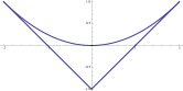
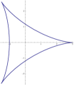
Figure 1: Regions for Koornwinder orthogonal polynomials. Left: $\mathrm{BC}_{2}$. Right: $\mathrm{A}_{2}$.

A related family of orthogonal polynomials 
Consider the family of weight functions defined by

$${\mathcal{W}}_{{\alpha},{\beta},{\gamma}}(x,y):=|x-y|^{2{\alpha}+1}|x+y|^{2{\beta}+1}(1-x^{2})^{\gamma}(1-y^{2})^{\gamma},\quad(x,y)\in[-1,1]^{2},$$ (58)

where ${\alpha},{\beta},{\gamma}>-1$, ${\alpha}+{\gamma}+\frac{3}{2}>0$ and ${\beta}+{\gamma}+\frac{3}{2}>0$. These weight functions are related to those in (51) by

$${\mathcal{W}}_{{\alpha},{\beta},{\gamma}}(x,y)=4^{\gamma}\,\big{|}x^{2}-y^{2}\big{|}\,W_{{\alpha},{\beta},{\gamma}}(2xy,x^{2}+y^{2}-1).$$

Let $\big{\{}P_{k,n}^{\,{\alpha},{\beta},{\gamma}}\big{\}}_{k=0}^{n}$ denote an orthogonal basis of ${\mathcal{V}}_{n}^{2}$ for $W_{{\alpha},{\beta},{\gamma}}$. Then an orthogonal basis of ${\mathcal{V}}_{2n}^{2}$ for ${\mathcal{W}}_{{\alpha},{\beta},{\gamma}}$ is given by

$$\begin{split}&P_{k,n}^{{\alpha},{\beta},{\gamma}}(2xy,x^{2}+y^{2}-1),\qquad 0\leq k\leq n,\\ &(x^{2}-y^{2})P_{k,n-1}^{{\alpha}+1,{\beta}+1,{\gamma}}(2xy,x^{2}+y^{2}-1),\,\,0\leq k\leq n-1,\end{split}$$ (59)

and an orthogonal basis of ${\mathcal{V}}_{2n+1}^{2}$ for ${\mathcal{W}}_{{\alpha},{\beta},{\gamma}}$ is given by

$$\begin{split}&(x+y)P_{k,n}^{{\alpha},{\beta}+1,{\gamma}}(2xy,x^{2}+y^{2}-1),\quad 0\leq k\leq n,\\ &(x-y)P_{k,n}^{{\alpha}+1,{\beta},{\gamma}}(2xy,x^{2}+y^{2}-1),\quad 0\leq k\leq n.\end{split}$$ (60)

In particular, when ${\gamma}=\pm\frac{1}{2}$, the basis can be given in terms of the Jacobi polynomials of one variable by using (56) and (57).

Jacobi polynomials associated with root system $\mathrm{A}_{2}$

These polynomials are orthogonal with respect to the weight function

$$W_{\alpha}(x,y):=\left[-3(x^{2}+y^{2}+1)^{2}+8(x^{3}-3xy^{2})+4\right]^{{\alpha}}$$ (61)

on the region bounded by $-3(x^{2}+y^{2}+1)^{2}+8(x^{3}-3xy^{2})+4=0$, which is called Steiner’s hypocycloid and can be described as the curve

$$x+iy=(2e^{i{\theta}}+e^{-2i{\theta}})/3.\qquad 0\leq{\theta}\leq 2\pi.$$

This three-cusped region is depicted in the right part of Figure 1. Apart from ${\alpha}=\pm\frac{1}{2}$, orthogonal polynomials with respect to $W_{\alpha}$ are not explicitly known. In the case of ${\alpha}=\pm\frac{1}{2}$, a basis of orthogonal polynomials can be given in homogeneous coordinates as follows. Let

$${\mathbb{R}}^{3}_{H}:=\big{\{}{\mathbf{t}}=(t_{1},t_{2},t_{3})\in{\mathbb{R}}^{3}\mid t_{1}+t_{2}+t_{3}=0\big{\}}.$$

For ${\mathbf{t}}\in{\mathbb{R}}^{3}_{H}$ and ${\mathbf{k}}=(k_{1},k_{2},k_{3})\in{\mathbb{R}}^{3}_{H}\cap{\mathbb{Z}}^{3}$, define $\phi_{\mathbf{k}}({\mathbf{t}})=e^{\tfrac{2\pi i}{3}{\mathbf{k}}\cdot{\mathbf{t}}}$ and

$${\mathsf{C}}^{\pm}_{\mathbf{k}}({\mathbf{t}}):=\tfrac{1}{6}\Big{(}\phi_{k_{1},k_{2},k_{3}}({\mathbf{t}})+\phi_{k_{2},k_{3},k_{1}}({\mathbf{t}})+\phi_{k_{3},k_{1},k_{2}}({\mathbf{t}})\pm\phi_{-k_{1},-k_{3},-k_{2}}({\mathbf{t}})\pm\phi_{-k_{2},-k_{1},-k_{3}}({\mathbf{t}})\pm\phi_{-k_{3},-k_{2},-k_{1}}({\mathbf{t}})\Big{)},$$

which are analogues of cosine and sine functions. The region bounded by Steiner’s hypocycloid is the image of the triangle $\Delta=\big{\{}(t_{1},t_{2})\in{\mathbb{R}}^{2}\mid t_{1},t_{2}\geq 0,\,t_{1}+t_{2}\leq 1\big{\}}$ under the change of variables $(t_{1},t_{2})\mapsto(x,y)$, defined by

$$z:=x+iy={\mathsf{C}}^{+}_{0,1,-1}({\mathbf{t}})=\tfrac{1}{3}\Big{(}\phi_{0,1,-1}({\mathbf{t}})+\phi_{1,-1,0}({\mathbf{t}})+\phi_{-1,0,1}({\mathbf{t}})\Big{)},$$ (62)

Under the change of variables (62), define

$$T_{k}^{n}(z,\bar{z}): ={\mathsf{C}}^{+}_{k,n-k,-n}({\mathbf{t}}),\qquad\qquad\;\;0\leq k\leq n,$$

$$U_{k}^{n}(z,\bar{z}): =\frac{{\mathsf{C}}^{-}_{k+1,n-k+1,-n-2}({\mathbf{t}})}{{\mathsf{C}}^{-}_{1,1,-2}({\mathbf{t}})},\qquad 0\leq k\leq m.$$

Then $\{T_{k}^{n}\}_{k=0}^{n}$ and $\{U_{k}^{n}\}_{k=0}^{n}$ are bases of ${\mathcal{V}}_{n}^{2}$ with respect to $W_{-\frac{1}{2}}$ and $W_{\frac{1}{2}}$, respectively. Both families of polynomials satisfy the relation $P_{n-k}^{n}(z,\bar{z})=\overline{P_{k}^{n}(z,\bar{z})}$, so that real-valued orthogonal bases can be derived from their real and imaginary parts. These polynomials are analogues of Chebyshev polynomials of the first and the second kind. They satisfy the following three-term relations:

$$P_{k}^{m+1}(z,\bar{z})=3zP_{k}^{m}(z,\bar{z})-P_{k+1}^{m}(z,\bar{z})-P_{k-1}^{m-1}(z,\bar{z})$$ (63)

for $0\leq k\leq m$ and $m\geq 1$, where

$$T_{-1}^{m}(z,\bar{z}):=T_{1}^{m+1}(z,\bar{z}),\quad T_{m+1}^{m}(z,\bar{z}):=T_{m}^{m+1}(z,\bar{z}),$$

$$U_{-1}^{m}(z,\bar{z}):=0,\quad U_{m}^{m-1}(z,\bar{z}):=0,$$

and, moreover,

$$T_{0}^{0}(z,\bar{z})=1,\quad T_{0}^{1}(z,\bar{z})=z,\quad T_{1}^{1}(z,\bar{z})=\bar{z},$$

$$U_{0}^{0}(z,\bar{z})=1,\quad U_{0}^{1}(z,\bar{z})=3z,\quad U_{1}^{1}(z,\bar{z})=3\bar{z}.$$

Further results and references  The Jacobi polynomials associated with $\mathrm{BC}_{2}$ and $\mathrm{A}_{2}$ were initially studied by Koornwinder [60, 61] (see also [62]), where it was shown that the orthogonal polynomials for $W_{{\alpha},{\beta},{\gamma}}$ in (51) are eigenfunctions of two commuting differential operators of second and fourth order, whereas the orthogonal polynomials associated with $\mathrm{A}_{2}$ are eigenfunctions of two commuting differential operators of second and third order. The two families are rank two cases of the Jacobi polynomials associated with root systems for general rank, the study of which was initiated by Heckman and Opdam, see Ch. 7. The Jacobi polynomials associated with $\mathrm{A}_{2}$ can be identified with Jack polynomials of two variables.

The special case of $P_{0}^{n}(x,y)$ of the first family when ${\gamma}=1/2$ was studied also in [30]. For further results on the first family, see [64] and [100], including explicit formula for $P_{k}^{n}$ in (54) given in terms of power series, and Rodrigues type formulas, and [134] where an explicit formula for the reproducing kernel in the case of $W$ in (55) with ${\gamma}=\pm 1/2$ was given in terms of the reproducing kernels of the orthogonal polynomials of one variable. For further results on the second family, see [98, 103] and [73], the latter one includes a connection with translation tiling and convergence of orthogonal expansions for $\mu=\pm\frac{1}{2}$.

Orthogonal polynomials with respect to $W_{\pm\frac{1}{2}}$ in (55) and the Jacobi polynomials associated with $\mathrm{A}_{2}$ when ${\gamma}=\frac{1}{2}$ are remarkable for having the maximum number of common zeros, i.e., ${\mathbb{P}}_{n}=\big{\{}P_{k}^{n}\mid 0\leq k\leq n\big{\}}$ has $\dim\Pi_{n-1}^{2}$ distinct real zeros ([73, 96]). By Theorem 2.15, Gaussian cubature formulas exist for these weight functions. For their generalizations to higher dimension, see §§1, 2.

The orthogonal polynomials with respect to ${\mathcal{W}}$ in (58) were studied in [134]. The reproducing kernel of $\Pi_{n}^{2}$ in $L^{2}({\mathcal{W}})$ can also be expressed in terms of the reproducing kernels of $\Pi_{n}^{2}$ in $L^{2}(W)$ for $W$ in (51). In particular, in the case of ${\gamma}=\pm\frac{1}{2}$, the kernel can be expressed in terms of the reproducing kernels of the Jacobi polynomials. When ${\gamma}=\pm\frac{1}{2}$, these weight functions admit minimal cubature rules that attain the lower bound (22).

7 Methods of constructing orthogonal polynomials of two variables from one variable

Let $w_{1}$ and $w_{2}$ be weight functions defined on the intervals $(a,b)$ and $(c,d)$, respectively. Let $\rho$ be a positive function on $(a,b)$. For the weight function

$$W(x,y):=w_{1}(x)w_{2}(\rho^{-1}(x)y),\qquad(x,y)\in\Omega,$$ (64)

where the domain $\Omega$ is defined by

$$\Omega:=\{(x,y)\in{\mathbb{R}}^{2}\mid a<x<b,\,\,\,c\rho(x)<y<d\rho(x)\},$$ (65)

a basis of orthogonal polynomials of two variables can be given in terms of orthogonal polynomials of one variable whenever either one of the following additional assumptions is satisfied:
Case 1.  $\rho$ is a polynomial of degree $1$;
Case 2.  $\rho=\sqrt{q}$ with $q$ a nonnegative polynomial of degree at most $2$, and further assume that $c=-d>0$ and $w_{2}$ is an even function on $(-c,c)$.
For each $k\in{\mathbb{N}}_{0}$ let $\{p_{n,k}\}_{n=0}^{\infty}$ denote the system of orthonormal polynomials with respect to the weight function $\big{(}\rho(x)\big{)}^{2k+1}w_{1}(x)$ on $(a,b)$. And let $\{q_{n}\}$ be the system of orthonormal polynomials with respect to $w_{2}(x)$ on $(c,d)$. Define polynomials of two variables by

$$P_{k}^{n}(x,y):=p_{n-k,k}(x)\,\big{(}\rho(x)\big{)}^{k}\,q_{k}\left(\frac{y}{\rho(x)}\right),\quad 0\leq k\leq n.$$ (66)

In Case 2 we see that $P_{k}^{n}$ are polynomials of degree $n$ because $q_{k}$ has the same parity as $k$ by evenness of $w_{2}$. Then $\{P_{k}^{n}\}_{k=0}^{n}$ is an orthonormal basis of ${\mathcal{V}}_{n}^{2}$ with respect to $W$ on $\Omega$.

Examples of orthogonal polynomials constructed by this method include product orthogonal polynomials, for which $\rho(x)=1$, and also the following cases:
Jacobi polynomials on the disk Let $w_{1}(x)=w_{2}(x):=(1-x^{2})^{\mu-1/2}$ on $[-1,1]$ and $\rho(x):=(1-x^{2})^{1/2}$. Then the weight function (64) and the basis (66) coincide up to constant factors with (36) and (37), respectively,
Jacobi polynomials on the triangle   Let $w_{1}(x):=x^{{\alpha}-\frac{1}{2}}(1-x)^{{\beta}+{\gamma}-1}$ and $w_{2}(x):=x^{{\beta}-\frac{1}{2}}(1-x)^{{\gamma}-\frac{1}{2}}$, both defined on the interval $(0,1)$, and let $\rho(x):=1-x$. Then the weight function (64) and the basis (66) coincide up to constant factors with (43) and (44), respectively.
Orthogonal polynomials on the parabolic domain Let $w_{1}(x):=x^{a}(1-x)^{b}$ on $[0,1]$, $w_{2}(x):=(1-x^{2})^{a}$ on $[-1,1]$, and $\rho(x):=\sqrt{x}$. Then the weight function (64) becomes

$$W_{a,b}(x,y):=(1-x)^{b}(x-y^{2})^{b},\qquad y^{2}<x<1.$$ (67)

The domain $\big{\{}(x,y)\mid y^{2}<x<1\big{\}}$ is bounded by a straight line and a parabola. The orthogonal polynomials $P_{k}^{n}$ in (66) are

$$P_{k}^{n}(x,y)=P_{n-k}^{(a,b+k+1/2)}(2x-1)\,x^{k/2}\,P_{k}^{(b,b)}\big{(}yx^{-1/2}\big{)},\quad 0\leq k\leq n.$$ (68)

Further results and references

This method of generating orthogonal polynomials of two variables first appeared in [69] and was used in [1] in certain special cases. It was presented systematically in [62], where the two cases for $\rho$ were stated. For further examples of explicit bases constructed in various domains, such as $\big{\{}(x,y)\mid x^{2}+y^{2}\leq 1,\;-a\leq y\leq b\big{\}}$ ($0<a,b<1$), see [103].

The sequence of polynomials in (68) satisfies a product formula [63] that generates a convolution structure for $L^{2}(W_{{\alpha},{\beta}})$, which was used to study the convergence of orthogonal expansions [15].

8 Other orthogonal polynomials of two variables

This subsection contains miscellaneous results on orthogonal polynomials of two variables.

1. Orthogonal polynomials for radial weight function. A weight function $W$ is called radial if it is of the form $W(x,y)=w(r)$, where $r=\sqrt{x^{2}+y^{2}}$. For such a weight function, an orthonormal basis can be given in polar coordinates $(x,y)=(r\cos{\theta},r\sin{\theta})$. Let $p_{m}^{(k)}$ denote the orthogonal polynomial of degree $m$ with respect to the weight function $r^{k+1}w(r)$ on $[0,\infty)$. Define

   $$\begin{split}P_{j,1}(x,y)&=p_{2j}^{(2n-4j+1)}(r)r^{(n-2j)}\cos\big{(}(n-2j){\theta}\big{)},\quad 0\leq j\leq n/2,\\ P_{j,2}(x,y)&=p_{2j}^{(2n-4j+1)}(r)r^{(n-2j)}\sin\big{(}(n-2j){\theta}\big{)},\quad 0\leq j<n/2.\end{split}$$ (69)

   Then $\{P_{j,1}\}_{j=0}^{\lfloor n/2\rfloor}\cup\{P_{j,2}\}_{j=0}^{\lfloor(n-1)/2\rfloor}$ is an orthogonal basis of ${\mathcal{V}}_{n}^{2}$ with respect to $W$. For $W(x,y)=(1-r^{2})^{\mu-1/2}$ this is the basis given in (39). Another example is the following:

   Product Hermite weight function $W(x,y)=e^{-x^{2}-y^{2}}$. The basis (69) is given by

   $$\begin{split}P_{j,1}(x,y)&=L_{j}^{n-2j}(r^{2})r^{(n-2j)}\cos\big{(}(n-2j){\theta}\big{)},\quad 0\leq j\leq n/2,\\ P_{j,2}(x,y)&=L_{2j}^{n-2j}(r^{2})ar^{(n-2j)}\sin\big{(}(n-2j){\theta}\big{)},\quad 0\leq j<n/2\end{split}$$ (70)

   in terms of Laguerre polynomials.

2. Bernstein–Szegő weight function of two variables. Let $m\in{\mathbb{N}}$. For any $i=0,\dots,m$ let $h_{i}(y)$ be polynomials in $y$ with real coefficients of degree at most $\frac{m}{2}-\big{|}\frac{m}{2}-i\big{|}$, with $h_{0}(y)=1$, such that, for all $y\in[-1,1]$,

   $$h(z,y)=\sum_{i=0}^{m}h_{i}(y)z^{i},\qquad z\in{\mathbb{C}},$$ (71)

   is nonzero whenever $|z|\leq 1$. Consider the two variable weight function

   $$W(x,y):=\frac{4}{\pi^{2}}\,\frac{\sqrt{1-x^{2}}\sqrt{1-y^{2}}}{|h(z,y)|^{2}},\qquad x=\tfrac{1}{2}(z+z^{-1}).$$ (72)

   For $\lceil\frac{m-2}{2}\rceil\leq k\leq n$, define the polynomials

   $$P_{k}^{n}(x,y)=U_{n-k}(y)\sum_{i=0}^{m}h_{i}(y)U_{k-i}(x),$$ (73)

   where it is understood that $U_{n}(x)=-U_{-n-2}(x)$ if $n<0$. Then $P_{k}^{n}$ is an orthogonal polynomial of degree $n$ with respect to $W$. In particular, if $m\leq 2$, then $\{P_{k}^{n}\}_{k=0}^{n}$ is an orthogonal basiof ${\mathcal{V}}_{n}^{2}$.

   Example $h(z,y)=1-2ayz+a^{2}z^{2}$, where $|a|<1$ and $a\in{\mathbb{R}}$. Then

   $$W(x,y)=\frac{4}{\pi^{2}}\,\frac{(1-a^{2})\sqrt{1-x^{2}}\sqrt{1-y^{2}}}{4a^{2}(x^{2}+y^{2})-4a(1+a^{2})xy+(1-a^{2})^{2}},$$ (74)

   The orthogonal polynomials in (73) are given, up to a constant, by $P_{0}^{n}(x,y)=U_{n}(y)$ and

   $$P_{k}^{n}(x,y)=\left(U_{k}(x)-2ayU_{k-1}(x)+a^{2}U_{k-2}(x)\right)U_{n-k}(y),\quad 1\leq k\leq n.$$

   For further examples and other properties of such polynomials, see [21].

3. Orthogonal polynomials on the regular hexagon. Orthogonal polynomials with respect to the constant weight function on the regular hexagon were studied in [25], An algorithm was given there for generating an orthogonal basis. No closed form of such a basis is known.

   4 Spherical harmonics

   Here and later we will use notation $\|x\|:=(x_{1}^{2}+\cdots+x_{d}^{2})^{1/2}$ and ${\langle}x,y{\rangle}:=x_{1}y_{1}+\cdots+x_{d}y_{d}$ ($x,y\in{\mathbb{R}}^{d}$). Spherical harmonics are an essential tool for Fourier analysis on the unit sphere $\SS^{d-1}:=\big{\{}x\in{\mathbb{R}}^{d}\mid\|x\|=1\big{\}}$ in ${\mathbb{R}}^{d}$ ($d\geq 2$). They are also building blocks for families of orthogonal polynomials with respect to radial weight functions on ${\mathbb{R}}^{d}$.

1 Ordinary spherical harmonics

Let $\Delta:=\frac{\partial^{2}}{\partial x_{1}^{2}}+\cdots+\frac{\partial^{2}}{\partial x_{d}^{2}}$ be the Laplace operator on ${\mathbb{R}}^{d}$. A polynomial $Y$ on ${\mathbb{R}}^{d}$ is called harmonic if $\Delta Y=0$. For $n=0,1,2,\ldots$ let $\mathcal{H}_{n}^{d}$ denote the linear space of homogeneous harmonic polynomials of degree $n$ in $d$ variables, i.e.,

$${\mathcal{H}}_{n}^{d}:=\left\{P\in{\mathcal{P}}_{n}^{d}\mid\Delta P=0\right\}.$$

By definition, a spherical harmonic is the restriction of a homogeneous harmonic polynomial to the unit sphere. If $Y\in{\mathcal{H}}_{n}^{d}$, then $Y(x)=\|x\|^{n}Y(x^{\prime})$ where $x^{\prime}=x/\|x\|\in\SS^{d-1}$. We shall also use ${\mathcal{H}}_{n}^{d}$ to denote the space of spherical harmonics of degree $n$. For $n\in{\mathbb{N}}_{0}$,

$$\dim{\mathcal{H}}_{n}^{d}=\dim{\mathcal{P}}_{n}^{d}-\dim{\mathcal{P}}_{n-2}^{d}=\binom{n+d-1}{d-1}-\binom{n+d-3}{d-1}=\frac{(2n+d-2)\,(n+d-3)!}{n!\,(d-2)!}.$$ (75)

Spherical harmonics of different degrees are orthogonal in $L^{2}(\SS^{d-1},d\sigma)$, where $d\sigma$ denotes the normalized spherical measure on $\SS^{d-1}$. There is a unique decomposition

$${\mathcal{P}}_{n}^{d}=\bigoplus_{j=0}^{\lfloor\frac{n}{2}\rfloor}\|x\|^{2j}{\mathcal{H}}_{n-2j}^{d}:\qquad P(x)=\sum_{j=0}^{\lfloor\frac{n}{2}\rfloor}\|x\|^{2j}Y_{n-2j}^{d}(x^{\prime}).$$

Orthonormal basis

In terms of spherical polar coordinates

$$\begin{cases}\quad x_{1}=r\sin\theta_{d-1}\ldots\sin\theta_{2}\sin\theta_{1},\\ \quad x_{2}=r\sin\theta_{d-1}\ldots\sin\theta_{2}\cos\theta_{1},\\ \quad\cdots\\ x_{d-1}=r\sin\theta_{d-1}\cos\theta_{d-2},\\ \quad x_{d}=r\cos\theta_{d-1},\end{cases}$$ (76)

where $r\geq 0$, $0\leq\theta_{1}<2\pi$, $0\leq\theta_{i}\leq\pi$ for $i=2,\ldots,d$, the normalized measure $d\sigma$ on $\SS^{d-1}$ is given by

$$d\sigma:={\omega}_{d}^{-1}\prod_{j=1}^{d-2}\big{(}\sin\theta_{d-j}\big{)}^{d-j-1}d\theta_{1}\,d\theta_{2}\ldots d\theta_{d-1},$$ (77)

where ${\omega}_{d}:=\frac{2\pi^{d/2}}{\Gamma(d/2)}$ is the surface area of $\SS^{d-1}$. For $d=2$, $\dim{\mathcal{H}}_{n}^{2}=2$. Then an orthogonal basis for ${\mathcal{H}}_{n}^{2}$ is given in polar coordinates by

$$Y_{n}^{(1)}(x):=r^{n}\cos(n\theta),\qquad Y_{n}^{(2)}(x):=r^{n}\sin(n\theta).$$

For $d>2$ and ${\alpha}\in{\mathbb{N}}_{0}^{d}$, define

$$Y_{\alpha}(x):=[h_{\alpha}]^{-1}r^{|\alpha|}g_{\alpha}(\theta_{1})\prod_{j=1}^{d-2}(\sin\theta_{d-j})^{|\alpha^{j+1}|}\,C_{\alpha_{j}}^{{\lambda}_{j}}(\cos\theta_{d-j}),$$ (78)

where $g_{\alpha}(\theta_{1}):=\cos(\alpha_{d-1}\theta_{1})$ (if $\alpha_{d}=0$) and $:=\sin((\alpha_{d-1}+1)\theta_{1})$ (if $\alpha_{d}=1$), where $|\alpha^{j}|:=\alpha_{j}+\ldots+\alpha_{d}$, ${\lambda}_{j}:=|\alpha^{j+1}|+(d-j-1)/2$, and where

$$[h_{\alpha}]^{2}:=b_{\alpha}\prod_{j=1}^{d-2}\frac{\alpha_{j}!\,\big{(}\tfrac{1}{2}(d-j+1)\big{)}_{|\alpha^{j+1}|}\,(\alpha_{j}+{\lambda}_{j})}{(2{\lambda}_{j})_{\alpha_{j}}\,\big{(}\tfrac{1}{2}(d-j)\big{)}_{|\alpha^{j+1}|}\,{\lambda}_{j}}$$

with $b_{\alpha}=2$ if $\alpha_{d-1}+\alpha_{d}>0$, else $=1.$ Then $\{Y_{\alpha}\}_{|\alpha|=n,\,\alpha_{d}=0,1}$ is an orthonormal basis of ${\mathcal{H}}_{n}^{d}$.

Projection opeator

The operator $\operatorname{proj}_{n}\colon L^{2}(\SS^{d-1},d\sigma)\to{\mathcal{H}}_{n}^{d}$ satisfies

$$\operatorname{proj}_{n}P(x)= \sum_{j=0}^{\lfloor\frac{n}{2}\rfloor}\frac{1}{4^{j}j!\,\big{(}-n+2-\tfrac{1}{2}d\big{)}_{j}}\,\|x\|^{2j}\Delta^{h}P(x)$$

$$= \frac{(-1)^{n}}{2^{n}\big{(}\tfrac{1}{2}d-1\big{)}_{n}}\,\|x\|^{2\|\alpha\|+d-2}P\left(\frac{\partial}{\partial x}\right)\left\{\|x\|^{-d+2}\right\}.$$ (79)

In particular, the projection of $x^{\alpha}$ is, up to a constant, Maxwell’s representation, defined by

$$H_{\alpha}(x):=\|x\|^{2|\alpha|+d-2}\frac{\partial^{\alpha}}{\partial x^{\alpha}}\left\{\|x\|^{-d+2}\right\},\quad\alpha\in{\mathbb{N}}_{0}^{d}.$$ (80)

The set $\{H_{\alpha}\}_{|\alpha|=n,\,\alpha_{d}=0,1}$ is a basis of ${\mathcal{H}}_{n}^{d}$. Furthermore, $H_{\alpha}$ satisfy a recursive relation

$$H_{\alpha+e_{i}}(x)=-(2|\alpha|+d-2)x_{i}H_{\alpha}(x)+\|x\|^{2}\frac{\partial}{\partial x_{i}}H_{\alpha}(x).$$ (81)

Let $P_{n}(\cdot,\cdot)$ denote the reproducing kernel of ${\mathcal{H}}_{n}^{d}$. Then the projection operator can be written as an integral operator

$$\operatorname{proj}_{n}f(x)=\frac{1}{{\omega}_{d}}\int_{\SS^{d-1}}f(y)P_{n}(x,y)\,d\sigma(y).$$

Reproducing kernel and zonal spherical harmonics

In terms of an orthonormal basis $\{Y_{j}\}_{j=1}^{\dim{\mathcal{H}}_{n}^{d}}$ of ${\mathcal{H}}_{n}^{d}$, the reproducing kernel, by definition, can be written as

$$P_{n}(x,y)=\sum_{1\leq j\leq\dim{\mathcal{H}}_{n}^{d}}Y_{j}(x)Y_{j}(y).$$ (82)

The kernel is invariant under the action of the orthogonal group $O(d)$ and it depends only on the distance between $x$ and $y$ on the sphere. Moreover,

$$P_{n}(x,y)=\frac{n+{\lambda}}{{\lambda}}\,C_{n}^{{\lambda}}\left({\langle}x,y{\rangle}\right),\quad x,y\in\SS^{d-1},\quad{\lambda}=\tfrac{1}{2}d-1.$$ (83)

For $y\in\SS^{d-1}$ fixed, both sides of (83) as a function of $x\in\SS^{d-1}$ are zonal spherical harmonics, i.e., spherical harmonics which are invariant under an orthogonal transformation leaving $y$ fixed. The corresponding homogeneous polynomial $\|x\|^{n}C_{n}^{(d-2)/2}\big{(}{\langle}x,y{\rangle}/\|x\|\big{)}$ is then called a zonal harmonic polynomial in $x\in{\mathbb{R}}^{d}$. The combination of (82) and (83) is known as the addition formula of spherical harmonics. The reproducing property of the kernel leads to the Funk–Hecke formula

$$\int_{\SS^{d-1}}f({\langle}x,y{\rangle})Y(x)\,d\sigma(x)={\lambda}_{n}Y(y),\quad Y\in{\mathcal{H}}_{n}^{d-1},\quad y\in\SS^{d-1},$$ (84)

for all functions $f$ for which the left-hand side is finite, where

$${\lambda}_{n}=\frac{1}{{\omega}_{d-1}}\int_{-1}^{1}f(t)\,\frac{C_{n}^{\lambda}(t)}{C_{n}^{\lambda}(1)}\,(1-t^{2})^{{\lambda}-\frac{1}{2}}\,dt,\quad{\lambda}=\tfrac{1}{2}d-1.$$

The Poisson summation kernel satisfies, for $x,y\in\SS^{d-1}$,

$$\sum_{n=0}^{\infty}P_{n}(x,y)r^{n}=\frac{1-r^{2}}{\big{(}1-{\langle}x,y{\rangle}r+r^{2}\big{)}^{\frac{1}{2}d}}=\frac{1-r^{2}}{\|\,rx-y\,\|^{d}}.$$ (85)

Laplace–Beltrami operator

This is the operator $\Delta_{0}$ defined by

$$(\Delta_{0}f)(x):=(\Delta F)(x),\quad x\in\SS^{d-1},$$ (86)

where $F(y):=f(y/\|y\|)$ is the extension of $f$ to ${\mathbb{R}}^{d}\backslash\{0\}$ which is homogeneous of degree 0. In terms of the spherical polar coordinates $x=rx^{\prime}$, $r>0$ and $x^{\prime}\in\SS^{d-1}$, the usual Laplace operator $\Delta$ is decomposed as

$$\Delta=\frac{d^{2}}{dr^{2}}+\frac{d-1}{r}\frac{d}{dr}+\frac{1}{r^{2}}\Delta_{0}.$$ (87)

The spherical harmonics are eigenfunctions of $\Delta_{0}$ :

$$\Delta_{0}Y=-n(n+d-2)Y,\qquad Y\in{\mathcal{H}}_{n}^{d}.$$ (88)

In terms of the spherical coordinates (76), $\Delta_{0}$ is given by

$$\Delta_{0}= \frac{1}{(\sin\theta_{d-1})^{d-2}}\frac{\partial}{\partial\theta_{d-1}}\left((\sin\theta_{d-1})^{d-2}\frac{\partial}{\partial\theta_{d-1}}\right)$$ (89)

$$+\sum_{j=1}^{d-2}\frac{1}{(\sin{\theta}_{d-1})^{2}\cdots(\sin\theta_{j+1})^{2}\sin^{j-1}\theta_{j}}\frac{\partial}{\partial\theta_{j}}\left((\sin\theta_{j})^{j-1}\frac{\partial}{\partial\theta_{j}}\right).$$

Furthermore, it satisfies a decomposition

$$\Delta_{0}=\sum_{1\leq i<j\leq d}\left(x_{i}\frac{\partial}{\partial x_{j}}-x_{j}\frac{\partial}{\partial x_{i}}\right)^{2}$$ (90)

for $x\in\SS^{d-1}$. The operator $A_{i,j}=x_{i}\frac{\partial}{\partial x_{j}}-x_{j}\frac{\partial}{\partial x_{i}}$ is the derivative with respect to the angle (Euler angle) in the polar coordinates of $(x_{i},x_{j})$-plane, and it is also the infinitesimal operator of the regular representation $f\mapsto f(Q^{-1}x)$ of the rotation group ${\rm SO}(d)$.

Further results and references

A number of books contain chapters or sections on spherical harmonics, treating the subject from various points of view. For earlier development, especially on $\SS^{2}$, see [48]. A well circulated early introductory is [86]. The connection to Fourier analysis in Euclidean space is treated in [101], see also [87]. For the connection to the Radon transform, see [46]. For applications in integral geometry, see [44]. For the point of view of group representations, see [108]. The fact that the zonal polynomial is of the form $p_{n}({\langle}x,y{\rangle})$ can be used as a starting point to study properties of Gegenbauer polynomials, see [86, 108] as well as [4]. Spherical harmonics are used as building blocks for orthogonal families on radial symmetric measures, see [28, 127] and the next section.

2 $h$-Harmonics for product weight functions on the sphere

A far reaching extension of spherical harmonics are Dunkl’s $h$-harmonics associated with reflection groups, see Chapter 7. We consider the case ${\mathbb{Z}}_{2}^{d}$, since explicit formulas are available mostly in this case. Let

$$w_{\kappa}(x):=c_{\kappa}\prod_{i=1}^{d}|x_{i}|^{2\kappa_{i}}\quad\hbox{with}\quad c_{\kappa}:=\frac{\pi^{\frac{1}{2}d}}{\Gamma\big{(}\tfrac{1}{2}d\big{)}}\,\frac{\Gamma\big{(}|\kappa|+\tfrac{1}{2}d\big{)}}{\Gamma\big{(}\kappa_{1}+\frac{1}{2}\big{)}\ldots\Gamma\big{(}\kappa_{d}+\frac{1}{2}\big{)}},\quad|\kappa|:=\kappa_{1}+\ldots+\kappa_{d},$$ (91)

normalized such that $\int_{\SS^{d-1}}w_{\kappa}(x)\,d\sigma=1$. This weight function is invariant under the group ${\mathbb{Z}}_{2}^{d}$, for which the results for ordinary spherical harmonics can be extended in explicit formulas.

Definition

The $h$-harmonics are homogeneous polynomials that satisfy $\Delta_{h}Y=0$, where

$$\Delta_{h}:={\mathcal{D}}_{1}^{2}+\ldots+{\mathcal{D}}_{d}^{2}$$ (92)

is the Dunkl Laplacian and ${\mathcal{D}}_{j}$, $1\leq j\leq d$, are the Dunkl operators associated with ${\mathbb{Z}}_{2}^{d}$,

$${\mathcal{D}}_{j}f(x):=\frac{\partial}{\partial x_{j}}f(x)+\kappa_{j}\frac{f(x)-f(x_{1},\ldots,-x_{j},\ldots,x_{d})}{x_{j}}.$$ (93)

The spherical $h$-harmonics are the restriction of $h$-harmonics to the sphere. Let ${\mathcal{H}}_{n}^{d}(w_{\kappa})$ denote the space of $h$-harmonics of degree $n$. Then

$$\Delta_{h,0}Y=-n(n+2|\kappa|+d-2)Y,\qquad Y\in{\mathcal{H}}_{n}^{d}(w_{\kappa}),$$ (94)

where $\Delta_{h,0}$ is the spherical $h$-Laplacian operator, and $\dim{\mathcal{H}}_{n}^{d}(w_{\kappa})=\dim{\mathcal{H}}_{n}^{d}$.

Orthonormal basis

A basis of ${\mathcal{H}}_{n}^{d}(w_{\kappa})$ can be given in spherical coordinates (76) and in terms of generalized Gegenbauer polynomials which are defined by

$$\begin{split}C_{2n}^{({\lambda},\mu)}(x)&:=\frac{\left({\lambda}+\mu\right)_{n}}{\big{(}\mu+\frac{1}{2}\big{)}_{n}}\,P_{n}^{({\lambda}-1/2,\mu-1/2)}(2x^{2}-1),\\ C_{2n+1}^{({\lambda},\mu)}(x)&:=\frac{\left({\lambda}+\mu\right)_{n+1}}{\big{(}\mu+\frac{1}{2}\big{)}_{n+1}}\,xP_{n}^{({\lambda}-1/2,\mu+1/2)}(2x^{2}-1).\end{split}$$ (95)

The polynomials $C_{n}^{({\lambda},\mu)}$ are orthogonal with respect to the weight function

$$w_{{\lambda},\mu}(x)=|x|^{2{\lambda}}(1-x^{2})^{\,\mu-1/2},\quad x\in[-1,1].$$

Let $h_{n}^{({\lambda},\mu)}:=c\int_{-1}^{1}\big{(}C_{n}^{({\lambda},\mu)}(t)\big{)}^{2}w_{{\lambda},\mu}(t)\,dt$, normalized such that $h_{0}^{({\lambda},\mu)}=1$. Then

$$\begin{split}h_{2n}^{({\lambda},\mu)}&=\frac{\big{(}{\lambda}+\frac{1}{2}\big{)}_{n}({\lambda}+\mu)_{n}}{n!\,\big{(}\mu+\frac{1}{2}\big{)}_{n}}\,\frac{{\lambda}+\mu}{{\lambda}+\mu+2n},\\ h_{2n+1}^{({\lambda},\mu)}&=\dfrac{\big{(}{\lambda}+\frac{1}{2}\big{)}_{n}\left({\lambda}+\mu\right)_{n+1}}{n!\,\big{(}\mu+\frac{1}{2}\big{)}_{n+1}}\,\frac{{\lambda}+\mu}{{\lambda}+\mu+2n+1}.\end{split}$$ (96)

For $d\geq 2$ and $\alpha\in{\mathbb{N}}_{0}^{d}$, define

$$Y_{\alpha}(x):=[h_{\alpha}]^{-1}r^{|\alpha|}g_{\alpha}(\theta_{1})\prod_{j=1}^{d-2}(\sin\theta_{d-j})^{|\alpha^{j+1}|}\,C_{\alpha_{j}}^{({\lambda}_{j},\kappa_{j})}(\cos\theta_{d-j}),$$ (97)

where $g_{\alpha}(\theta):=C_{\alpha_{d-1}}^{(\kappa_{d},\kappa_{d-1})}(\cos\theta)$ (if $\alpha_{d}=0$) and $:=\sin\theta\,C_{\alpha_{d-1}-1}^{(\kappa_{d}+1,\kappa_{d-1})}(\cos\theta)$ if ($\alpha_{d}=1$), and where $|\alpha^{j}|:=\alpha_{j}+\ldots+\alpha_{d}$,   $|\kappa^{j}|:=\kappa_{j}+\ldots+\kappa_{d}$,   ${\lambda}_{j}:=|\alpha^{j+1}|+|\kappa^{j+1}|+\tfrac{1}{2}(d-j-1)$,   and

$$\left[h_{\alpha}^{n}\right]^{2}:=\frac{a_{\alpha}}{\big{(}|\kappa|+\tfrac{1}{2}d\big{)}_{n}}\prod_{j=1}^{d-1}h_{\alpha_{i}}^{({\lambda}_{i},\kappa_{i})}(\kappa_{i}+{\lambda}_{i})_{\alpha_{i}},\quad a_{\alpha}:=\begin{cases}1&\hbox{if $\alpha_{d}=0$}\\ \kappa_{d}+\frac{1}{2}&\hbox{if $\alpha_{d}=1$}\end{cases}.$$

Then $\{Y_{\alpha}\}_{|\alpha|=n,\,\alpha_{d}=0,1}$ is an orthonormal basis of ${\mathcal{H}}_{n}^{d}(w_{\kappa})$.

Reproducing kernel

The reproducing kernel of ${\mathcal{H}}_{n}^{d}(w_{\kappa})$ is given by

$$P_{n}(w_{\kappa};x,y)=\sum_{1\leq j\leq\dim{\mathcal{H}}_{n}^{d}(w_{\kappa})}Y_{j}(x)Y_{j}(y)$$

where $\{Y_{j}\}_{j=1}^{\dim{\mathcal{H}}_{n}^{d}(w_{\kappa})}$ is an orthonormal basis of ${\mathcal{H}}_{n}^{d}(w_{\kappa})$. It satisfies a closed formula

$$P_{n}(w_{\kappa};x,y)=\frac{n+|\kappa|+\frac{1}{2}d-1}{|\kappa|+\frac{1}{2}d-1}\int_{[-1,1]^{d}}C_{n}^{|\kappa|+\frac{1}{2}d-1}\big{(}x_{1}y_{1}t_{1}+\cdots+x_{d}y_{d}t_{d}\big{)}\\ \times\left({\textstyle\prod\limits_{i=1}^{d}}c_{\kappa_{i}}(1+t_{i})(1-t_{i}^{2})^{\kappa_{i}-1}\right)dt.$$ (98)

Further results and references

The $h$-harmonics associated with a finite reflection group were first studied by Dunkl in [26]. Next he defined his Dunkl operators in [27]. For an overview of the extensive theory of $h$-harmonics, see [28] and Chapter 7. The case ${\mathbb{Z}}_{2}^{d}$ was studied in detail in [119], which contains (97) and (98), as well as a closed formula for an analog of the Poisson integral. A Funk–Hecke type formula was given in [123]. For a monic $h$-harmonic basis and a biorthogonal basis, see [128]. For a connection to products of Heine–Stieltjes polynomials, see [110].

5 Classical orthogonal polynomials of several variables

General properties of orthogonal polynomials of several variables were given in §2. This section contains results for specific weight functions.

1 Classical orthogonal polynomials on the unit ball

On the unit ball $B^{d}:=\{x\in{\mathbb{R}}^{d}:\mid\|x\|\leq 1\}$, consider the weight function

$$W_{\mu}(x,y):=\frac{\Gamma\big{(}\mu+\frac{1}{2}(d+1)\big{)}}{\pi^{d/2}\Gamma\big{(}\mu+\frac{1}{2}\big{)}}\,(1-\|x\|^{2})^{\mu-\frac{1}{2}},\quad\mu>-\tfrac{1}{2},$$ (99)

normalized such that its integral over $B^{d}$ is 1. For $d=2$, see §2.

Differential operator

Orthogonal polynomials of degree $n$ with respect to $W_{\mu}$ are eigenfunctions of a second order differential operator:

$$\left(\Delta-{\textstyle\sum\limits_{j=1}^{d}}\,\frac{\partial}{\partial x_{j}}\,x_{j}\left((2\mu-1)+{\textstyle\sum\limits_{i=1}^{d}}x_{i}\frac{\partial}{\partial x_{i}}\right)\right)P=-(n+d)(n+2\mu-1)P,\quad P\in{\mathcal{V}}_{n}^{d},$$ (100)

where $\Delta$ is the Laplace operator.

First orthonormal basis

Associated with $x=(x_{1},\ldots,x_{d})\in{\mathbb{R}}^{d}$, define ${\mathbf{x}}_{j}:=(x_{1},\ldots,x_{j})$ for $1\leq j\leq d$ and ${\mathbf{x}}_{0}:=0$. For ${\alpha}\in{\mathbb{N}}_{0}^{d}$ and $1\leq j\leq d$, let ${\alpha}^{j}:=({\alpha}_{j},\ldots,{\alpha}_{d})$ and ${\alpha}^{d+1}:=0$. An orthonormal basis $\{P_{\alpha}\}_{|{\alpha}|=n}$ of ${\mathcal{V}}_{n}^{d}$ is given by

$$P_{\alpha}(x):=[h_{\alpha}]^{-1}\prod_{j=1}^{d}\big{(}1-\|{\mathbf{x}}_{j-1}\|^{2}\big{)}^{\frac{1}{2}\alpha_{j}}\,C_{\alpha_{j}}^{{\lambda}_{j}}\biggl{(}\frac{x_{j}}{(1-\|{\mathbf{x}}_{j-1}\|^{2})^{1/2}}\biggl{)},$$ (101)

where ${\lambda}_{j}:=\mu+|\alpha^{j+1}|+\frac{1}{2}(d-j)$ and $h_{\alpha}$ is given by

$$[h_{\alpha}]^{2}:=\frac{\big{(}\mu+\frac{1}{2}d\big{)}_{|{\alpha}|}}{\big{(}\mu+\frac{1}{2}(d+1)\big{)}_{|{\alpha}|}}\prod_{j=1}^{d}\frac{\big{(}\mu+\frac{1}{2}(d-j)\big{)}_{|{\alpha}^{j}|}\,\big{(}2\mu+2|\alpha^{j+1}|+d-j\big{)}_{{\alpha}_{j}}}{\big{(}\mu+\frac{1}{2}(d-j+1)\big{)}_{|{\alpha}^{j}|}\,{\alpha}_{j}!},$$ (102)

and where the case $\mu=0$ can be obtained as a limit for $\mu\to 0$ by using (32), similarly as for (37), (38).

Second orthonormal basis

Let $r_{k}^{d}:=\dim{\mathcal{H}}_{k}^{d}$. For $0\leq j\leq n/2$ let $\big{\{}Y_{\ell,n-2j}\mid 1\leq\ell\leq r_{n-2j}^{d}\big{\}}$ be an orthonormal basis of ${\mathcal{H}}_{n-2j}^{d}$, the space of spherical harmonics of degree $n-2j$, with respect to the normalized surface measure. For $0\leq j\leq n/2$, define

$$P_{\ell,j}(x):=[h_{j,n}]^{-1}P_{j}^{(\mu-\frac{1}{2},n-2j+\frac{1}{2}d-1)}\big{(}2\|x\|^{2}-1\big{)}\,Y_{\ell,n-2j}(x),$$ (103)

where

$$[h_{j,n}]^{2}:=\frac{\big{(}\mu+\frac{1}{2}\big{)}_{j}\,\big{(}\frac{1}{2}d\big{)}_{n-j}}{j!\,\big{(}\mu+\frac{1}{2}(d+1)\big{)}_{n-j}}\,\frac{\big{(}n-j+\mu+\frac{1}{2}(d-1)\big{)}}{\big{(}n+\mu+\frac{1}{2}(d-1)\big{)}}.$$

Then $\big{\{}P_{\ell,j}\mid 1\leq\ell\leq r_{n-2j}^{d},\;0\leq j\leq n/2\big{\}}$ is an orthonormal basis of ${\mathcal{V}}_{n}^{d}$.

Appell’s biorthogonal polynomials

These are two families of polynomials yielding bases $\big{\{}U_{\alpha}\}_{|{\alpha}|=n}$ and $\big{\{}V_{\alpha}\}_{|{\alpha}|=n}$ of ${\mathcal{V}}_{n}^{d}$, where the second basis is the monic basis, up to constant factors, and the first basis is biorthogonal to it.

1. The family $\{U_{\alpha}\}$ is defined by the generating function

   $$\Big{(}\big{(}1-{\langle}b,x{\rangle}\big{)}^{2}+\|b\|^{2}\big{(}1-\|x\|^{2}\big{)}\Big{)}^{-\mu}=\sum_{\alpha\in{\mathbb{N}}_{0}^{d}}b^{\alpha}U_{\alpha}(x),\qquad b\in{\mathbb{R}}^{d},\;\|b\|<1.$$ (104)

   It satisfies the Rodrigues type formula,

   $$U_{\alpha}(x)=\frac{(-1)^{|\alpha|}\,(2\mu)_{|\alpha|}}{2^{|\alpha|}\,\big{(}\mu+\frac{1}{2}\big{)}_{|\alpha|}\,\alpha!}\,\big{(}1-\|x\|^{2}\big{)}^{-\mu+\frac{1}{2}}\,\frac{\partial^{|\alpha|}}{\partial x^{\alpha}}\,\big{(}1-\|x\|^{2}\big{)}^{|\alpha|+\mu-\frac{1}{2}}.$$ (105)

   where $\frac{\partial^{|{\alpha}|}}{\partial x^{\alpha}}:=\frac{\partial^{|\alpha|}}{\partial x_{1}^{\alpha_{1}}\ldots\partial x_{d}^{{\alpha}_{d}}}$. Furthermore, it can be explicitly given as

   $$U_{\alpha}(x) =\frac{(2\mu)_{|\alpha|}}{\alpha!}\sum_{\beta\leq\alpha}\frac{(-1)^{|\beta|}\,(-\alpha)_{2\beta}}{2^{2|\beta|}\,\beta!\,\big{(}\mu+\frac{1}{2}\big{)}_{|\beta|}}\,x^{\alpha-2\beta}\big{(}1-\|x\|^{2}\big{)}^{|\beta|}$$ (106)

   $$=\frac{(2\mu)_{|\alpha|}x^{\alpha}}{\alpha!}\,F_{B}\Big{(}-\tfrac{1}{2}\alpha,-\tfrac{1}{2}(\alpha-\mathbf{1});\mu+\tfrac{1}{2};x_{1}^{-2}\big{(}1-\|x\|^{2}\big{)},\ldots,x_{d}^{-2}\big{(}1-\|x\|^{2}\big{)}\Big{)},$$

   where $(-{\alpha})_{2{\beta}}:=(-\alpha_{1})_{2\beta_{1}}\ldots(-\alpha_{d})_{2\beta_{d}}$, $\mathbf{1}:=(1,\ldots,1)$, $\beta\leq\alpha$ means $\beta_{i}\leq\alpha_{i}$ ($1\leq i\leq d$), and $F_{B}$ is Lauricella’s hypergeometric series of type $B$ (see [34] and Chapter 3).

2. The family $\{V_{\alpha}\}$ is defined by the generating function

   $$\big{(}1-2{\langle}b,x{\rangle}+\|b\|^{2}\big{)}^{-\mu-(d-1)/2}=\sum_{\alpha\in{\mathbb{N}}_{0}^{d}}b^{\alpha}V_{\alpha}(x),\qquad b\in{\mathbb{R}}^{d},\;\|b\|<1.$$ (107)

   The generating function implies that

   $$\|b\|^{n}\,C_{n}^{\mu+\frac{1}{2}(d-1)}\left(\frac{{\langle}b,x{\rangle}}{\|b\|}\right)=\sum_{|{\alpha}|=n}b^{\alpha}V_{\alpha}(x).$$ (108)

   The polynomial $V_{\alpha}$ can be written explicitly as

   $$V_{\alpha}(x) =2^{|\alpha|}x^{\alpha}\sum_{\gamma<\alpha}\frac{\big{(}\mu+\tfrac{1}{2}(d-1)\big{)}_{|\alpha|-|\gamma|}\,(-\alpha+\gamma)_{\gamma}}{(\alpha-\gamma)!\,\gamma!}\,2^{-2|\gamma|}x^{-2\gamma}$$ (109)

   $$=\frac{2^{|\alpha|}\big{(}\mu+\frac{1}{2}(d-1)\big{)}_{|\alpha|}}{\alpha!}\,x^{\alpha}F_{B}\Big{(}-\tfrac{1}{2}\alpha,-\tfrac{1}{2}(\alpha-\mathbf{1});-|\alpha|-\mu-\tfrac{1}{2}(d-3);x_{1}^{-2},\ldots,x_{d}^{-2}\Big{)}.$$

Neither $\{U_{\alpha}\}_{{\alpha}|=n}$ nor $\{V_{\alpha}\}_{|{\alpha}|=n}$ is an orthogonal basis of ${\mathcal{V}}_{n}^{d}$, but the two bases are biorthogonal to each other:

$$\int_{B^{d}}V_{\alpha}(x)U_{\beta}(x)W_{\mu}(x)\,dx=\frac{\mu+\tfrac{1}{2}(d-1)}{|\alpha|+\mu+\tfrac{1}{2}(d-1)}\,\frac{(2\mu)_{|\alpha|}}{\alpha!}\,\delta_{\alpha,\beta}.$$ (110)

The monic basis For each ${\alpha}$, define

$$R_{\alpha}(x):=\frac{\alpha!}{2^{|\alpha|}\big{(}\mu+\tfrac{1}{2}(d-1)\big{)}_{|\alpha|}}\,V_{\alpha}(x).$$ (111)

Then the polynomials $R_{\alpha}$ ($|{\alpha}|=n$) form a monic basis of ${\mathcal{V}}_{n}^{d}$, i.e., $R_{\alpha}(x)=x^{\alpha}-Q_{\alpha}(x)$ with $Q_{\alpha}\in\Pi_{n-1}^{d}$. The $L^{2}(W_{\mu},B^{d})$ norm, $\|\cdot\|_{2,\mu}$, of $R_{\alpha}$ is the error of the best approximation of $x^{\alpha}$, which satisfies a closed formula

$$\min_{P\in\Pi_{n-1}^{d}}\|x^{\alpha}-P(x)\|_{2,\mu}^{2}=\|R_{\alpha}\|_{2,\mu}^{2}=\frac{{\lambda}\,\alpha!}{2^{n-1}({\lambda})_{n}}\int_{0}^{1}{\textstyle\prod\limits_{i=1}^{d}}P_{\alpha_{i}}(t)\,t^{n+2{\lambda}-1}\,dt,$$ (112)

where ${\lambda}=\mu+(d-1)/2>0$, $n=|\alpha|$, and $P_{{\alpha}_{i}}$ is the Legendre polynomial.
Reproducing kernel The kernel $P_{n}(\cdot,\cdot)$ of ${\mathcal{V}}_{n}^{d}$ with respect to $W_{\mu}$, defined in (25), satisfies a compact formula. For $\mu>0$, $x,y\in B^{d}$,

$$P_{n}(x,y)=c_{\mu}\frac{2n+2\mu+d-1}{2\mu+d-1}\int_{-1}^{1}C_{n}^{\mu+\frac{1}{2}(d-1)}\left({\langle}x,y{\rangle}+t{\textstyle\sqrt{1-\|x\|^{2}}\sqrt{1-\|y\|^{2}}}\,\right)(1-t^{2})^{\mu-1}\,dt,$$ (113)

where $[c_{\mu}]^{-1}:=\int_{-1}^{1}(1-t^{2})^{\mu-1}dt$. For $\mu=0$, $x,y\in B^{d}$ this degenerates to

$$P_{n}(x,y)=\frac{n+\frac{1}{2}(d-1)}{d-1}\sum_{\epsilon=0,1}C_{n}^{\frac{1}{2}(d-1)}\left({\langle}x,y{\rangle}+(-1)^{\epsilon}{\textstyle\sqrt{1-\|x\|^{2}}\sqrt{1-\|y\|^{2}}}\,\right).$$ (114)

These formulas are essential for obtaining sharp results for convergence of orthogonal expansions. When $\mu=\frac{1}{2}(m-1)$, (113) can also be written as

$$P_{n}(x,y)=\frac{2n+m+d-2}{m+d-2}\int_{\SS^{m-1}}C_{n}^{\frac{1}{2}(m+d)-1}\left({\langle}x,y{\rangle}+{\textstyle\sqrt{1-\|x\|^{2}}\sqrt{1-\|y\|^{2}}}\,{\langle}\xi,e_{1}{\rangle}\right)d{\sigma}_{m}(\xi),$$ (115)

where $d\sigma_{m}$ is the normalized surface measure on $\SS^{m-1}$.

For the constant weight $W_{1/2}(x)=(d+1)/\pi$, there is another formula for the reproducing kernel,

$$P_{n}(x,y)=(2nd^{-1}+1)\int_{\SS^{d-1}}C_{n}^{d/2}\big{(}{\langle}x,\xi{\rangle}\big{)}\,C_{n}^{d/2}\big{(}{\langle}\xi,y{\rangle}\big{)}\,d\sigma_{d}(\xi).$$ (116)

Further results and references

For orthogonal bases on the ball, see [5, 28, 33]. There are further results on biorthogonal bases, see [5, 33]. For the monic basis, see [128]. Orthogonal bases consisting of ridge polynomials were discussed in [123], together with a Funk–Hecke type formula for orthogonal polynomials. The compact formulas (113) and (114) for the reproducing kernels were proved in [122] and used to study expansion problems, whereas the compact formula (115) was proved in [124, Theorem 2.6] (there take $H_{2}(\eta)=1$). Formula (116) was proved in [91] in the context of approximation by ridge functions, and in [132] in connection with Radon transforms. In [7] three-term relations are used to develop an efficient numerical algorithm for the evaluation of orthogonal polynomials in (101) with $d=2,3$. For convergence and summability of orthogonal expansions, see §7.

2 Classical orthogonal polynomials on the simplex

For $x\in{\mathbb{R}}^{d}$, let $|x|:=x_{1}+\cdots+x_{d}$. Let $T^{d}:=\{x\in{\mathbb{R}}^{d}\mid x_{1},\ldots,x_{d},1-|x|\geq 0\}$ be the simplex in ${\mathbb{R}}^{d}$. The classical weight function on $T^{d}$ is defined by

$$W_{\kappa}(x):=\frac{\Gamma\big{(}|\kappa|+\tfrac{1}{2}(d+1)\big{)}}{\prod_{i=1}^{d+1}\Gamma\big{(}\kappa_{i}+\tfrac{1}{2}\big{)}}\,x_{1}^{\kappa_{1}-\frac{1}{2}}\ldots x_{d}^{\kappa_{d}-\frac{1}{2}}(1-|x|)^{\kappa_{d+1}-\frac{1}{2}},\quad\kappa_{1},\ldots,\kappa_{d+1}>-\tfrac{1}{2}.$$ (117)

Differential operator

Orthogonal polynomials of degree $n$ with respect to $W_{\kappa}$ are eigenfunctions of a second order differential operator,

$$\left(\sum_{i=1}^{d}x_{i}(1-x_{i})\,\frac{\partial^{2}}{\partial x_{i}^{2}}-2\sum_{1\leq i<j\leq d}x_{i}x_{j}\,\frac{\partial^{2}}{\partial x_{i}\partial x_{j}}+\sum_{i=1}^{d}\left(\big{(}\kappa_{i}+\tfrac{1}{2}\big{)}-\big{(}|\kappa|+\tfrac{1}{2}(d+1)\big{)}x_{i}\right)\frac{\partial}{\partial x_{i}}\right)P\\ =-n\left(n+|\kappa|+\tfrac{1}{2}(d-1)\right)P,\qquad P\in{\mathcal{V}}_{n}^{d},$$ (118)

where $|\kappa|=\kappa_{1}+\cdots+\kappa_{d+1}$.

An orthonormal basis

To state this basis we use the notation of ${\mathbf{x}}_{j}$ and $\alpha^{j}$ as in the first orthonormal basis on $B^{d}$ of §1. We also put $\kappa^{j}:=(\kappa_{j},\ldots,\kappa_{d+1})$ ($j=0,1,\ldots,d+1$) if $\kappa=(\kappa_{1},\ldots,\kappa_{d+1})$. Then an orthonormal basis $\{P_{\alpha}\}_{|{\alpha}|=n}$ of ${\mathcal{V}}_{n}^{d}$ is given by

$$P_{\alpha}(x):=[h_{\alpha}]^{-1}\prod_{j=1}^{d}\big{(}1-|{\mathbf{x}}_{j-1}|\big{)}^{\alpha_{j}}\,P_{\alpha_{j}}^{(a_{j},\kappa_{j}-\frac{1}{2})}\left(\frac{2x_{j}}{1-|{\mathbf{x}}_{j-1}|}-1\right),$$ (119)

where $a_{j}:=2|\alpha^{j+1}|+|\kappa^{j+1}|+\tfrac{1}{2}(d-j-1)$ and $h_{\alpha}$ is given by

$$[h_{\alpha}]^{2}:=\prod_{j=1}^{d}\frac{\big{(}\kappa_{j}+\frac{1}{2}\big{)}_{{\alpha}_{j}}\,\big{(}|\kappa^{j+1}|+\frac{1}{2}(d-j+1)\big{)}_{|\alpha^{j}|+|\alpha^{j+1}|}}{\alpha_{j}!\,\big{(}|\kappa^{j}|+\frac{1}{2}(d-j+2)\big{)}_{|\alpha^{j}|+|\alpha^{j+1}|}}\,\frac{2(a_{j}+\kappa_{j}+{\alpha}_{j})+1}{2(a_{j}+\kappa_{j}+2{\alpha}_{j})+1}.$$

Appell’s biorthogonal polynomials

These are two families of polynomials yielding bases $\big{\{}U_{\alpha}\}_{|{\alpha}|=n}$ and $\big{\{}V_{\alpha}\}_{|{\alpha}|=n}$ of ${\mathcal{V}}_{n}^{d}$, where the second basis is the monic basis and the first basis is biorthogonal to it.
(i) The family $\{U_{\alpha}\}$ is defined by the Rodrigues type formula

$$U_{\alpha}(x):=x_{1}^{-\kappa_{1}+\frac{1}{2}}\ldots x_{d}^{-\kappa_{d}+\frac{1}{2}}\big{(}1-|x|\,\big{)}^{-\kappa_{d+1}+\frac{1}{2}}\,\frac{\partial^{|\alpha|}}{\partial x^{\alpha}}\left(x_{1}^{\alpha_{1}+\kappa_{1}-\frac{1}{2}}\ldots x_{d}^{\alpha_{d}+\kappa_{d}-\frac{1}{2}}(1-|x|)^{|\alpha|+\kappa_{d+1}-\frac{1}{2}}\right).$$ (120)

(ii) The family $\{V_{\alpha}\}$ is explicitly defined by

$$V_{\alpha}(x) :=\sum_{\beta\leq\alpha}(-1)^{n+|\beta|}\left({\textstyle\prod\limits_{i=1}^{d}}\,\binom{\alpha_{i}}{\beta_{i}}\,\frac{\big{(}\kappa_{i}+\frac{1}{2}\big{)}_{\alpha_{i}}}{\big{(}\kappa_{i}+\frac{1}{2}\big{)}_{\beta_{i}}}\right)\,\frac{\big{(}|\kappa|+\frac{1}{2}(d-1)\big{)}_{n+|\beta|}}{\big{(}|\kappa|+\frac{1}{2}(d-1)\big{)}_{n+|\alpha|}}\,x^{\beta}$$

$$=\frac{(-1)^{n}\big{(}\kappa+\frac{\bf 1}{2}\big{)}_{\alpha}}{\big{(}n+|\kappa|+\frac{1}{2}(d-1)\big{)}_{|\alpha|}}\,F_{A}\left(n+|\kappa|+\tfrac{1}{2}(d-1),-\alpha;\kappa+\tfrac{\bf 1}{2},x\right)$$ (121)

where $F_{A}$ denotes Lauricella’s hypergeometric series of type A (see [34] and Chapter 3).

Neither $\{U_{\alpha}\}_{{\alpha}|=n}$ nor $\{V_{\alpha}\}_{|{\alpha}|=n}$ is an orthogonal basis of ${\mathcal{V}}_{n}^{d}$, but the two bases are biorthogonal to each other:

$$\int_{T^{d}}V_{\beta}(x)U_{\alpha}(x)W_{\kappa}(x)\,dx=\frac{\big{(}\kappa+\frac{1}{2}\big{)}_{\alpha}\big{(}\kappa_{d+1}+\frac{1}{2}\big{)}_{|\alpha|}}{\big{(}|\kappa|+\frac{1}{2}(d+1)\big{)}_{2|\alpha|}}\,\alpha!\,\delta_{\alpha,\beta}.$$ (122)

Monic orthogonal basis

By (2) and (122) the polynomials $V_{\alpha}$ ($|{\alpha}|=n$) form a monic basis: $V_{\alpha}(x)=x^{\alpha}-Q_{\alpha}(x)$, $Q_{\alpha}\in\Pi_{n-1}^{d}$. Such polynomials can be defined more generally in view of the observation that the simplex $T^{d}$ is associated with the permutation group of $X:=(x_{1},\ldots,x_{d},x_{d+1})$, where $x_{d+1}=1-|x|$. For $x\in T^{d}$ and ${\alpha}\in{\mathbb{N}}_{0}^{d+1}$, define $X^{\alpha}:=x_{1}^{{\alpha}_{1}}\ldots x_{d}^{{\alpha}_{d}}(1-|x|)^{{\alpha}_{d+1}}$. For $|{\alpha}|=n$ let $R_{\alpha}(x)=X^{\alpha}-Q_{\alpha}(x)$ be the element of ${\mathcal{V}}_{n}^{d}$ such that $Q_{\alpha}$ is a polynomial of degree at most $|{\alpha}|-1$. When ${\alpha}_{d+1}=0$, $R_{\alpha}(x)$ agrees with $V_{\alpha}(x)$ in (2) up to a constant factor. The $L^{2}(W_{\kappa},T^{d})$ norm $\|\cdot\|_{2,\kappa}$ of $R_{\alpha}$ is the error of the best approximation of $X^{\alpha}$, which satisfies a closed formula:

$$\min_{P\in\Pi_{n-1}^{d}}\|X^{\alpha}-P(x)\|_{2,\kappa}^{2}=\|V_{\alpha}\|_{2,\kappa}^{2}=\frac{\big{(}|\kappa|+\frac{1}{2}(d-1)\big{)}\big{(}\kappa+\frac{\mathbf{1}}{2}\big{)}_{\alpha}}{\big{(}|\kappa|+\frac{1}{2}(d-1\big{)}_{2|\alpha|}}\int_{0}^{1}\left({\textstyle\prod\limits_{i=1}^{d+1}}P_{\alpha_{i}}^{(0,\kappa_{i}-\frac{1}{2})}(2t-1)\right)t^{|\alpha|+|\kappa|+\frac{d-3}{2}}\,dt.$$ (123)

If ${\alpha}_{d+1}=0$, (123) gives the error of best approximation to $x^{\alpha}$.

Reproducing kernel

The kernel $P_{n}(\cdot,\cdot)$ of ${\mathcal{V}}_{n}^{d}$ with respect to $W_{\kappa}$, defined in (25), satisfies a compact formula. For $\kappa_{i}>0$, $1\leq i\leq d$, $x,y\in T^{d}$,

$$P_{n}(x,y)=c_{\kappa}\,\frac{2(2n+|{\kappa}|)+d-1}{2|{\kappa}|+d-1}\,\frac{\big{(}|{\kappa}|+\frac{1}{2}(d-1)\big{)}_{n}}{\big{(}\frac{1}{2}\big{)}_{n}}\\ \times\int_{[-1,1]^{d+1}}P_{n}^{(|{\kappa}|+(d-2)/2,-1/2)}\left(2z(x,y,t)^{2}-1\right)\left({\textstyle\prod\limits_{i=1}^{d+1}}(1-t_{i}^{2})^{{\kappa}_{i}-1}\right)dt,$$ (124)

where $z(x,y,t):=\sqrt{x_{1}y_{1}}\,t_{1}+\cdots+\sqrt{x_{d}y_{d}}\,t_{d}+\sqrt{1-|x|}\sqrt{1-|y|}\,t_{d+1}$ and

$$[c_{\kappa}]^{-1}:=\int_{[-1,1]^{d+1}}\left({\textstyle\prod\limits_{i=1}^{d+1}}(1-t_{i}^{2})^{{\kappa}_{i}-1}\right)dt.$$

If some $\kappa_{i}=0$, then the formula holds under the limit relation

$$\lim_{{\lambda}\to 0}c_{\lambda}\int_{-1}^{1}g(t)(1-t)^{{\lambda}-1}\,dt=\tfrac{1}{2}\big{(}g(1)+g(-1)\big{)}.$$

Further results and references

For $d=2$ the polynomials $U_{\alpha}$ on $T^{d}$ were defined in [5] and the polynomials $V_{\alpha}$ were studied in [35]. For $d>2$ they appeared in [45] when $W_{\kappa}(x)=1$, and in [28] in general. The monic basis of polynomials $R_{\alpha}$ was studied in [128]. The formula (124) of the reproducing kernel appeared in [121]. A product formula for orthogonal polynomials on the simplex was established in [63]. The polynomials in (119) serve as generating functions for the Hahn polynomials in several variables [59, 136]. For convergence and summability of orthogonal expansions see §7.

3 Hermite polynomials of several variables

These are orthogonal polynomials with respect to the product weight

$$W_{H}(x):=\pi^{-d/2}e^{-\|x\|^{2}},\qquad x\in{\mathbb{R}}^{d}.$$ (125)

Many properties are inherited from Hermite polynomials of one variable.

Differential operator

Orthogonal polynomials of degree $n$ with respect to $W_{H}$ are eigenfunctions of a second order differential operator:

$$\left(\Delta-2\sum_{i=1}^{d}x_{i}\,\frac{\partial}{\partial x_{i}}\right)P=-2nP,\qquad P\in{\mathcal{V}}_{n}^{d}.$$ (126)

Product orthogonal basis

For $\alpha\in{\mathbb{N}}_{0}^{d}$, define

$$H_{\alpha}(x):=H_{{\alpha}_{1}}(x_{1})\ldots H_{{\alpha}_{d}}(x_{d}).$$ (127)

Then $\big{\{}[c_{\alpha}]^{-1}H_{\alpha}\big{\}}_{|{\alpha}|=n}$ is an orthonormal basis of ${\mathcal{V}}_{n}^{d}$, where $[c_{\alpha}]^{2}:=2^{|\alpha|}\alpha!$. As products of Hermite polynomials of one variable, they inherit a generating function and Rodrigues type formula. Furthermore, they satisfy

$$\sum_{|\alpha|=n}\frac{H_{\alpha}(y)}{\alpha!}\,x^{\alpha}=\frac{1}{n!\,\pi^{\frac{1}{2}}}\int_{-\infty}^{\infty}H_{n}\Big{(}{\langle}x,y{\rangle}+s\sqrt{1-\|x\|^{2}}\,\Big{)}\,e^{-s^{2}}\,ds,\quad x\in{\mathbb{B}}^{d},\;y\in{\mathbb{R}}^{d}.$$

In particular,

$$\sum_{|\alpha|=n}\frac{H_{\alpha}(y)}{\alpha!}\,x^{\alpha}=\frac{1}{n!}\,H_{n}\big{(}{\langle}x,y{\rangle})\big{)},\qquad\|x\|=1,\;y\in{\mathbb{R}}^{d}.$$ (128)

Second orthonormal basis

For $0\leq j\leq n/2$ and $r_{k}^{d}:=\dim{\mathcal{H}}_{k}^{d}$ let $\{Y_{\ell,n-2j}\}_{\ell=1}^{r_{n-2j}^{d}}$ be an orthonormal basis of ${\mathcal{H}}_{n-2j}^{d}$ as in (103). Define

$$P_{\ell,j}^{n}(x):=[c_{j,n}]^{-1}L_{j}^{n-2j+\frac{1}{2}(d-2)}\big{(}\|x\|^{2}\big{)}\,Y_{\ell,n-2j}(x),\qquad[c_{j,n}]^{2}:=\frac{\big{(}\frac{1}{2}d\big{)}_{n-j}}{j!}.$$ (129)

Then $\big{\{}P_{\ell,j}^{n}\mid 1\leq\ell\leq r_{n-2j}^{d},\;0\leq j\leq\frac{1}{2}n\big{\}}$ is an orthonormal basis of ${\mathcal{V}}_{n}^{d}$.

Mehler formula

The reproducing kernel $P_{n}(\cdot,\cdot)$ of ${\mathcal{V}}_{n}^{d}$, as defined in (25), satisfies, for $0<z<1$ and $x,y\in{\mathbb{R}}^{d}$,

$$\sum_{n=0}^{\infty}P_{n}(x,y)\,z^{n}=\frac{1}{(1-z^{2})^{d/2}}\,\exp\left(-\frac{z^{2}(\|x\|^{2}+\|y\|^{2})-2z{\langle}x,y{\rangle}}{1-z^{2}}\right).$$ (130)

Further results and references

The study of Hermite polynomials of several variables was started by Hermite and followed by many other authors, see [5, 33] for references. Analogues of Hermite polynomials can be defined more generally for the weight function

$$W(x)=(\det A)^{\frac{1}{2}}\,\pi^{-d/2}\,\exp\left(-x^{\mathsf{tr}}Ax\right),$$ (131)

where $A$ is a positive definite matrix. Two families of biorthogonal polynomials can be defined for $W$ in (131), which coincide when $A$ is an identity matrix. These were studied in [5], see also [33]. Since $A$ is positive definite, it can be written as $A=B^{\mathsf{tr}}B$. Thus, orthogonal polynomials for $W$ in (131) can be derived from Hermite polynomials for $W_{H}$ by a change of variables.

4 Laguere and generalized Hermite polynomials

Laguerre polynomials of several variables

Put $|x|:=x_{1}+\cdots x_{d}$ and ${\mathbb{R}}_{+}^{d}:=\big{\{}x\in{\mathbb{R}}^{d}\mid x_{1},\ldots,x_{d}\geq 0\big{\}}$. Laguerre polynomials of several variables are orthogonal polynomials with respect to the weight function

$$W_{L}(x):=\frac{1}{\prod_{k=1}^{d}\Gamma(\kappa_{i}+\tfrac{1}{2})}\,x^{\kappa}e^{-|x|},\qquad x\in{\mathbb{R}}_{+}^{d},$$ (132)

which can be written as a product of weight functions in one variable. Many properties are inherited from Laguerre polynomials of one variable.

The polynomials in ${\mathcal{V}}_{n}$ are eigenfunctions of a differential operator:

$$\left(\sum_{i=1}^{d}x_{i}\,\frac{\partial^{2}}{\partial x_{i}^{2}}+\sum_{i=1}^{d}(\kappa_{i}+1-x_{i})\,\frac{\partial}{\partial x_{i}}\right)P=-nP,\qquad P\in{\mathcal{V}}_{n}^{d}.$$ (133)

An orthonormal basis of ${\mathcal{V}}_{n}^{d}$ is given by $\{L_{\alpha}^{\kappa}\}_{|{\alpha}|=n}$, where

$$\textstyle L^{\kappa}_{\alpha}(x):=\binom{\alpha+\kappa}{\alpha}^{-1/2}L_{{\alpha}_{1}}^{\kappa_{1}}(x_{1})\ldots L_{{\alpha}_{d}}^{\kappa_{d}}(x_{d})$$ (134)

The reproducing kernel $P_{n}(\cdot,\cdot)$ of ${\mathcal{V}}_{n}^{d}$, defined in (25), satisfies, for $0<z<1$ and $x,y\in{\mathbb{R}}_{+}^{d}$,

$$\sum_{n=0}^{\infty}P_{n}(x,y)\,z^{n}=(1-z)^{-1}\prod_{i=1}^{d}\exp\left(-\frac{z(x_{i}+y_{i})}{1-z}\right)\,(x_{i}y_{i}z)^{-\frac{1}{2}\kappa_{i}}\,I_{\kappa_{i}}\left(\frac{2\sqrt{x_{i}y_{i}z}}{1-z}\right),$$ (135)

where $I_{\kappa}$ denote the modified Bessel function of order $\kappa$.

Generalized Hermite polynomials of several variables

These are orthogonal polynomials with respect to the product weight function

$$W_{\kappa}(x):=\prod_{i=1}^{d}|x_{i}|^{2\kappa_{i}}e^{-x_{i}^{2}}$$ (136)

Let $\Delta_{h}$ be the Dunkl Laplacian (92). The orthogonal polynomials in ${\mathcal{V}}_{n}^{d}$ are eigenfunctions of a differential-difference operator:

$$\Big{(}\Delta_{h}-2{\langle}x,\nabla{\rangle}\Big{)}P=-2nP,\qquad P\in{\mathcal{V}}_{n}^{d}.$$ (137)

For $\kappa>0$ let the generalized Hermite polynomials $H_{n}^{\kappa}$ in one variable be defined by

$$\begin{split}H_{2n}^{\kappa}(x)&:=(-1)^{n}2^{2n}n!\,L_{n}^{\kappa-\frac{1}{2}}(x^{2}),\\ H_{2n+1}^{\kappa}(x)&:=(-1)^{n}2^{2n+1}n!\,x\,L_{n}^{\kappa+\frac{1}{2}}(x^{2}).\end{split}$$ (138)

Let $h_{n}^{\kappa}=\Gamma\big{(}\kappa+\frac{1}{2}\big{)}^{-1}\int_{\mathbb{R}}[H_{n}^{\kappa}(x)]^{2}x^{\kappa}e^{-x^{2}}\,dx$, normalized such that $h_{0}^{\kappa}=1$. Then

$$h_{2n}^{\kappa}=2^{4n}n!\,(\mu+\tfrac{1}{2})_{n}\quad\hbox{and}\quad h_{2n+1}^{\kappa}=2^{4n+2}n!\,(\mu+\tfrac{1}{2})_{n+1}.$$ (139)

An orthonormal basis of ${\mathcal{V}}_{n}^{d}$ for $W_{\kappa}$ is given by $\{P_{\alpha}\}_{|\alpha|=n}$, where

$$P_{\alpha}(x):=\big{(}h_{\alpha_{1}}^{\kappa_{1}}\ldots h_{\alpha_{d}}^{\kappa_{d}}\big{)}^{-\frac{1}{2}}H_{\alpha_{1}}^{\kappa_{1}}(x_{1})\cdots H_{\alpha_{d}}^{\kappa_{d}}(x_{d}).$$ (140)

Another orthonormal basis, analogous to (129), can be given, in polar coordinates, by Laguerre polynomials and $h$-harmonics.

Further results and references

As products of Laguerre polynomials of one variable, the polynomials $L^{\kappa}_{\alpha}(x)$ in (134) have a generating function, a Rodrigues type formula, as well as a product formula that induces a convolution structure. The generalized Hermite polynomials can be defined for weight functions under other reflection groups. For those and further properties of these functions, including a Mehler type formula, see [28, 95, 125].

5 Jacobi polynomials of several variables

These polynomials are orthogonal with respect to the weight function

$$W_{a,b}(x):=\prod_{i=1}^{d}(1-x_{i})^{a_{i}}(1+x_{i})^{b_{i}},\quad x\in[-1,1]^{d}.$$ (141)

An orthogonal basis is formed by the product Jacobi polynomials,

$$P_{\alpha}(x):=P_{{\alpha}_{1}}^{(a_{1},b_{1})}(x_{1})\ldots P_{{\alpha}_{d}}^{(a_{d},b_{d})}(x_{d}),\quad{\alpha}\in{\mathbb{N}}_{0}^{d}.$$

Most results for these orthogonal polynomials follow from properties of Jacobi polynomials of one variable. The reproducing kernel $P_{n}(\cdot,\cdot)$ of ${\mathcal{V}}_{n}^{d}$ satisfies

$$\sum_{n=0}^{\infty}P_{n}(x,{\bf 1})r^{n}=\prod_{i=1}^{d}\frac{(1-r)(1+r)^{a_{i}-b_{i}+1}}{(1-2rx_{i}+r^{2})^{a_{i}+3/2}}\;\,\mbox{}_{2}F_{1}\left(\genfrac{}{}{0.0pt}{}{\frac{1}{2}(b_{i}-a_{i}),\frac{1}{2}(b_{i}-a_{i}-1)}{b_{i}+1};\frac{2r(1+x_{i})}{(1+r)^{2}}\right),$$ (142)

where $0<r<1$ and $\mathbf{1}=(1,\ldots,1)$.

In the case of the product Chebyshev weight function, i.e., $a_{i}=b_{i}=-\frac{1}{2}$, $i=1,\ldots,d$, the reproducing kernel $P_{n}(\cdot,\cdot)$ satisfies a closed formula [28, Theorem 9.6.3]. This is given in terms of a divided difference $[x_{1},\ldots,x_{d}]f$ defined by

$$[x_{0}]\,f:=f(x_{0})\quad\hbox{and}\quad[x_{0},\ldots,x_{n}]\,f:=\frac{[x_{0},\ldots,x_{n-1}]\,f-[x_{1},\ldots,x_{n}]\,f}{x_{0}-x_{n}},$$

which is a symmetric function in $x$. For $W(x):=\prod_{i=1}^{d}(1-x_{i}^{2})^{-\frac{1}{2}}$,

$$P_{n}(x,\mathbf{1})=[x_{1},\ldots,x_{d}]\,G_{n},$$ (143)

where

$$G_{n}(t):=2(-1)^{\left[\frac{1}{2}(d+1)\right]}\,(1-t^{2})^{\frac{1}{2}(d-1)}\begin{cases}T_{n}(t)&\hbox{for $d$ even},\cr U_{n-1}(t)&\hbox{for $d$ odd}.\end{cases}$$

The product Jacobi polynomials inherite a product formula from the one-variable case [28, Lemma 9.6.1], which allows one to define a convolution structure for orthogonal expansions.

6 Relation between orthogonal polynomials on classical domains

By classical domains we mean the sphere, ball, simplex, ${\mathbb{R}}^{d}$ and ${\mathbb{R}}_{+}^{d}$. Orthogonal polynomials on these domains are closely related.

1 Orthogonal polynomials on the sphere and on the ball

A nonnegative weight function $H$ defined on ${\mathbb{R}}^{d+1}$ is called $S$-symmetric if $H(x^{\prime},x_{d+1})=H(x^{\prime},-x_{d+1})=H(-x^{\prime},x_{d+1})$, where $x^{\prime}\in{\mathbb{R}}^{d}$, and if the restriction $W_{H}$ of $H$ on the sphere $\SS^{d}$ is a non-trivial weight function. Let ${\mathcal{H}}_{n}^{d+1}(H)$ denote the space of homogeneous polynomials of degree $n$ that are orthogonal in $L^{2}(\SS^{d},H)$ to polynomials of lower degrees. Then, just as in the case (75) of $H=1$,

$$\dim{\mathcal{H}}_{n}^{d+1}(H)=\dim{\mathcal{P}}_{n}^{d+1}-\dim{\mathcal{P}}_{n-2}^{d+1}=\binom{n+d}{d}-\binom{n+d-2}{d}.$$ (144)

Associated with an $S$-symmetric weight function $H$, define

$$W_{H}(x):=H\Big{(}x,\big{(}1-\|x\|^{2}\big{)}^{\frac{1}{2}}\Big{)},\quad x\in{\mathbb{B}}^{d},$$

which is a centrally symmetric weight function on the ball. Let $\{P_{\alpha}\}_{|\alpha|=n,\,\alpha\in{\mathbb{N}}_{0}^{d}}$ be an orthogonal basis for ${\mathcal{V}}_{n}^{d}$ with respect to $(1-\|x\|^{2})^{-\frac{1}{2}}W_{H}(x)$, and let $\{Q_{\beta}\}_{|\beta|=n-1,\,\beta\in{\mathbb{N}}_{0}^{d}}$ be an orthogonal basis for ${\mathcal{V}}_{n-1}^{d}$ with respect to the weight function $(1-\|x\|^{2})^{\frac{1}{2}}W_{H}(x)$. For $y\in{\mathbb{R}}^{d+1}$ define

$$y=r\,(x,x_{d+1}),\qquad x\in{\mathbb{B}}^{d},\quad(x,x_{d+1})\in\SS^{d},\quad r\geq 0.$$

For $\alpha,\beta\in{\mathbb{N}}_{0}^{d}$, $|\alpha|=n$ and $|\beta|=n-1$, define

$$Y_{\alpha}^{(1)}(y)=r^{n}P_{\alpha}(x)\quad\hbox{and}\quad Y_{\beta}^{(2)}(y)=r^{n}x_{d+1}Q_{\beta}(x).$$

Theorem 6.1.

The functions $Y_{\alpha}^{(1)}$ and $Y_{\beta}^{(2)}$ are homogeneous polynomials of degree $n$ in the variable $y$. Furthermore, $\big{\{}Y_{\alpha}^{(1)}\big{\}}_{|\alpha|=n}\cup\big{\{}Y_{\beta}^{(2)}\big{\}}_{|\beta|=n-1}$ is an orthogonal basis for ${\mathcal{H}}_{n}^{d+1}(H)$.

Let $P_{n}^{H}(\cdot,\cdot)$ denote the reproducing kernel of ${\mathcal{H}}_{n}^{d}(H)$ and let $P_{n}(\cdot,\cdot)$ denote the reproducing kernel of ${\mathcal{V}}_{n}^{d}$ with respect to $(1-\|x\|^{2})^{-\frac{1}{2}}W_{H}(x)$. Then

$$P_{n}(x,y)=\tfrac{1}{2}\left(P_{n}^{H}\big{(}(x,x_{d+1}),(y,y_{d+1})\big{)}+P_{n}^{H}\big{(}(x,x_{d+1}),(y,-y_{d+1})\big{)}\right),$$ (145)

where $x_{d+1}=(1-\|x\|^{2})^{\frac{1}{2}}$ and $y_{d+1}=(1-\|y\|^{2})^{\frac{1}{2}}$. The relation is based on

$$\int_{\SS^{d}}f(y)\,d\omega(y)=\int_{{\mathbb{B}}^{d}}\left(f\big{(}x,(1-\|x\|^{2})^{\frac{1}{2}}\big{)}+f(x,-(1-\|x\|^{2})^{\frac{1}{2}}\big{)}\right)\,(1-\|x\|^{2})^{-\frac{1}{2}}\,dx,$$ (146)

where $d\omega$ is the Lebesgue measure (not normalized) on $\SS^{d}$. A further relation between orthogonal polynomials on ${\mathbb{B}}^{d}$ and those on $\SS^{d+m-1}$ follows from

$$\int_{\SS^{d+m-1}}f(y)\,d\omega(y)=\int_{{\mathbb{B}}^{d}}(1-\|x\|^{2})^{\frac{1}{2}(m-1)}\left(\int_{\SS^{m}}f\big{(}x,(1-\|x\|^{2})^{\frac{1}{2}}\xi\big{)}\,d\omega_{m}(\xi)\right)\,dx.$$

As a consequence of these relations, properties of the orthogonal polynomials with respect to the weight function

$$W_{\kappa}(x)=\prod_{i=1}^{d}|x_{i}|^{2\kappa_{i}}(1-\|x\|^{2})^{k_{d+1}-\frac{1}{2}},\quad k_{i}\geq 0,$$ (147)

on ${\mathbb{B}}^{d}$ can be derived from $h$-harmonics with respect to $w_{\kappa}(x)=\prod_{i=1}^{d+1}|x_{i}|^{2\kappa_{i}}$ on the sphere $\SS^{d+1}$. In particular, following (97) and using generalized Gegenbauer polynomials (95), define

$$P_{\alpha}(x):=[h_{\alpha}]^{-1}\prod_{j=1}^{d}(1-\|{\mathbf{x}}_{j-1}\|^{2})^{\frac{1}{2}\alpha_{j}}\,C_{\alpha_{j}}^{(a_{j},\kappa_{j})}\left(\big{(}1-\|{\mathbf{x}}_{j-1}\|^{2}\big{)}^{-\frac{1}{2}}x_{j}\right),\quad\alpha\in{\mathbb{N}}_{0}^{d},$$ (148)

where $|\alpha^{j}|:=\alpha_{j}+\ldots\alpha_{d}$, $|\kappa^{j}|:=\kappa_{j}+\ldots\kappa_{d+1}$, $a_{j}:=|\alpha^{j+1}|+|\kappa^{j+1}|+\frac{d-j}{2}$, and

$$\left[h_{\alpha}^{n}\right]^{2}:=\frac{1}{\big{(}|\kappa|+\frac{1}{2}(d+1)\big{)}_{n}}\prod_{j=1}^{d}h_{\alpha_{i}}^{({\alpha}_{i},\kappa_{i})}(\kappa_{i}+a_{i})_{\alpha_{i}}.$$

Then $\{P_{\alpha}\}_{|\alpha|=n}$ is an orthonormal basis of ${\mathcal{V}}_{n}^{d}$. A second orthonormal basis can be given in spherical-polar coordinates, analogous to (103) but using $h$-harmonics. The orthogonal polynomials in ${\mathcal{V}}_{n}^{d}$ are eigenfunctions of a second order differential-difference operator,

$$\left(\Delta_{h}-{\langle}x,\nabla{\rangle}^{2}-(2|\kappa|+d-1){\langle}x,\nabla{\rangle}\right)P=-n(n+2|\kappa|+d-1)\,P,$$ (149)

where $\Delta_{h}$ is the Dunkl Laplacian given in §2. The reproducing kernel $P_{n}(\cdot,\cdot)$ of ${\mathcal{V}}_{n}^{d}$ for $W_{\kappa}$ satisfies a closed formula:

$$P_{n}(x,y)=\frac{2n+2|\kappa|+d-1}{2|\kappa|+d-1}\,\int_{[-1,1]^{d+1}}C_{n}^{|\kappa|+\frac{1}{2}(d-1)}(x_{1}y_{1}t_{1}+\cdots+x_{d+1}y_{d+1}t_{d+1})\\ \times\left({\textstyle\prod\limits_{i=1}^{d}}(1+t_{i})\right)\,\left({\textstyle\prod\limits_{i=1}^{d+1}}c_{\kappa_{i}}\big{(}1-t_{i}^{2}\big{)}^{\kappa_{i}-1}\right)\,dt,$$ (150)

where $x_{d+1}=\sqrt{1-\|x\|^{2}}$ and $y_{d+1}=\sqrt{1-\|y\|^{2}}$.

Further results and references

The relation between orthogonal polynomials on the sphere and on the ball was explored in [120, 124]. The orthonormal basis (148) and the closed form of formula (150) were given in [124]. The monic orthogonal basis for $W_{\kappa}$ was studied in [128].

2 Orthogonal polynomials on the ball and on the simplex

Let $W$ be a weight function defined on the simplex $T^{d}$. Define

$$W_{T}(x):={W(x)}/{\sqrt{x_{1}\cdots x_{d}}}\quad\hbox{and}\quad W_{B}(x):=W(x_{1}^{2},\ldots,x_{d}^{2})$$

on $T^{d}$ and on the ball ${\mathbb{B}}^{d}$, respectively. There is a close relation between orthogonal polynomials for $W_{T}$ and those for ${\mathbb{B}}^{d}$. Let ${\mathcal{V}}_{n}^{d}(W)$ denote the space of orthogonal polynomials of degree $n$ with respect to $W$. Furthermore, let ${\mathcal{V}}_{n}(W_{B},{\mathbb{Z}}_{2}^{d})$ denote the subspace of ${\mathcal{V}}_{n}^{d}(W_{B})$ which contains polynomials that are invariant under ${\mathbb{Z}}_{2}^{d}$, that is, even in each variable. Then the mapping

$$\psi\colon T^{d}\to{\mathbb{B}}^{d}\colon(x_{1},\ldots,x_{d})\mapsto(x_{1}^{2},\ldots,x_{d}^{2})$$

induces a ono-to-one correspondence between $R\in{\mathcal{V}}_{n}^{d}(W_{T})$ and $R\circ\psi\in{\mathcal{V}}_{n}(W_{B},{\mathbb{Z}}_{2}^{d})$. This is based on the relation

$$\int_{B^{d}}f(x_{1}^{2},\ldots,x_{d}^{2})\,dx=\int_{T^{d}}f(u_{1},\ldots,u_{d})\,\frac{du}{\sqrt{u_{1}\cdots u_{d}}}.$$ (151)

Let $P_{n}(W;\cdot,\cdot)$ denote the reproducing kernel of ${\mathcal{V}}_{n}^{d}(W)$. Then the correspondence also extends to the reproducing kernel:

$$P_{n}(W_{T};x,y)=2^{-d}\sum_{\varepsilon\in{\mathbb{Z}}_{2}^{d}}P_{n}(W_{B};x^{1/2},\varepsilon y^{1/2}),$$ (152)

where $x^{1/2}:=\big{(}x_{1}^{1/2},\ldots,x_{d}^{1/2}\big{)}$. In particular, the identity (124) can be deduced from (150) by this relation.

Essentially all properties of orthogonal polynomials for $W_{T}$ can be deduced from the corresponding results for $W_{B}$. In particular, all results in §2 can be deduced from the corresponding results with respect to $W_{\kappa}$ in (147). In combination with §1 there is also a correspondence between orthogonal polynomials on the simplex and those on the sphere.

Further results and references

The relation between orthogonal polynomials on the ball and on the simplex was studied in [121]. The details on orthogonal systems for the classical weight functions were worked out in [125]. The connection extends to other aspects of analysis, including orthogonal expansion, approximation, and numerical integration.

3 Limit relations

Two limit relations between orthogonal polynomials on two different domains are worth mentioning.

Limit of orthogonal polynomials on the ball

[28, Theorem 8.3.5]
Let $P_{\alpha}(W_{\kappa})$ be the orthogonal polynomials (148) on the ball for $W_{\kappa}$ in (147). Then

$$\lim_{\kappa_{d+1}\to 0}P_{\alpha}(W_{\kappa},x/\kappa_{d+1})=c_{\alpha}^{-1}H_{\alpha_{1}}^{\kappa_{1}}(x_{1})\ldots H_{\alpha_{d}}^{\kappa_{d}}(x_{d}),$$

where the right-hand side is the generalized Hermite polynomial (140) on ${\mathbb{R}}^{d}$, a product of generalized Hermite polynomials in one variable.

Limit of orthogonal polynomials on the simplex

[28, Theorem 8.4.5]
Let $P_{\alpha}(W_{\kappa})$ be the orthogonal polynomials in (119) on the simplex for $W_{\kappa}$ in (117). Then

$$\lim_{\kappa_{d+1}\to 0}P_{\alpha}(W_{\kappa},x/\kappa_{d+1})=L_{\alpha_{1}}^{\kappa_{1}}(x_{1})\cdots L_{\alpha_{d}}^{\kappa_{d}}(x_{d})S_{\!n}$$

where the right-hand side is a Laguerre polynomial (134) on ${\mathbb{R}}_{+}^{d}$, a product of Laguerre polynomials of one variable.

7 Orthogonal expansions and summability

As long as polynomials are dense in $L^{2}(d\mu)$, the standard Hilbert space theory shows that the partial sum $S_{\!n}f$ in (28) converges to $f$ in $L^{2}(d\mu)$ norm. The convergence does not hold in general for $S_{\!n}f$ in other norms. The summability of the orthogonal expansions is often studied via the Cesàro means. For $\delta>0$, the Cesàro $(C,\delta)$ means of the orthogonal expansion (26) is defined by

$$S_{\!n}^{\delta}f(x):={\textstyle\binom{n+\delta}{n}^{-1}}\sum_{k=0}^{n}\binom{n-k+\delta-1}{n-k}\,S_{k}f(x).$$ (153)

There are many results for orthogonal expansions for classical type orthogonal polynomials. Below is a list of highlights with references.

Orthogonal expansions on $\SS^{d-1}$

The results are stated in terms of $w_{\kappa}$ defined in (91) on the sphere. The case $\kappa=0$ gives the result for ordinary spherical harmonics expansions. Let $\|\cdot\|_{\kappa,p}$ denote the $L^{p}(w_{\kappa})$ norm; for $p=\infty$, the norm is the uniform norm of $C(\mathbb{S}^{d-1})$. Let

$${\sigma}_{\kappa}:=\tfrac{d-2}{2}+|{\kappa}|-\min_{1\leq j\leq d}{\kappa}_{j},\quad{\delta}_{\kappa}(p):=\max\Big{(}(2{\sigma}_{\kappa}+1)\,\big{|}\tfrac{1}{p}-\tfrac{1}{2}\big{|}-\tfrac{1}{2},0\Big{)}.$$

1. For $p=1$ or $\infty$, the norm of partial sum operator and the projection operator satisfy $\|S_{\!n}\|_{{\kappa},p}\sim\|\operatorname{proj}_{n}\|_{{\kappa},p}\sim n^{{\sigma}_{\kappa}}$.

2. The $(C,\delta)$ means $S_{\!n}^{\delta}f\geq 0$ for all $f\geq 0$ if and only if $\delta\geq 2|{\kappa}|+d-1$.

3. If $f\in C(\SS^{d-1})$ then $S_{\!n}^{\delta}f$ converges to $f$ pointwise in $\{x\in\mathbb{S}^{d-1}\mid x_{1}\ldots x_{d}\neq 0\}$ if ${\delta}>\frac{d-1}{2}$; if $f\in L^{1}(w_{\kappa})$ then $S_{\!n}^{\delta}f$ converges almost everywhere to $f$ on $\SS^{d-1}$ if ${\delta}>{\sigma}_{\kappa}$.

4. For $p=1$ or $\infty$, $S_{\!n}^{\delta}f$ converges to $f$ in $L^{p}(w_{\kappa})$ if and only if $\delta>\sigma_{\kappa}$.

5. If $f\in L^{p}(w_{\kappa})$, $1\leq p\leq\infty$, $\big{|}\frac{1}{p}-\frac{1}{2}\big{|}\geq\frac{1}{2{\sigma}_{\kappa}+2}$ and ${\delta}>{\delta}_{\kappa}(p)$, then $S_{\!n}^{\delta}f$ converges to $f$ in $L^{p}(w_{\kappa}^{2})$.

For expansions of ordinary spherical harmonics, these were mostly proved in [14, 99], see [33] for earlier results. For $h$-harmonics, these results were established in [18, 19, 75, 118]. A comprehensive account that includes many more results is given in the monograph [20].

Orthogonal expansions on ${\mathbb{B}}^{d}$ and $T^{d}$

For orthogonal expansions with respect to $W_{\kappa}$ in (147) on the ball ${\mathbb{B}}^{d}$ and $W_{\kappa}$ in (117) on the simplex $T^{d}$, analogues of the above results hold. In fact, if we replace ${\sigma}_{\kappa}$ by

$${\sigma}_{\kappa}:=\tfrac{d-1}{2}+|{\kappa}|-\min_{1\leq j\leq d+1}{\kappa}_{j},$$

then all five properties hold with obvious modification. This is no accident, the three cases are intimately connected: some of the results on one domain can be deduced from the corresponding results on one of the other two domains. The study of summability on the ball started in [122]. The connection between the three domains was first applied in the study of orthogonal expansions in [124, 125], and next in full power in [18, 19, 75]. See [33, Ch. 12] for earlier results on orthogonal expansions and [20] for further results.

Orthogonal expansions on $[-1,1]^{d}$.

On $[-1,1]^{d}$ we consider the orthogonal expansions in the product Jacobi polynomials for $W_{a,b}$ in (141).

1. Let $a_{j}>-1$, $b_{j}>-1$ and $a_{j}+b_{j}\geq-1$ for $1\leq j\leq d$. For $f$ in $L^{p}(W_{a,b};[-1,1]^{d})$, $1\leq p<\infty$, or in $C([-1,1]^{d})$, the $(C,\delta)$ means $S_{\!n}^{\delta}f$ converges to $f$ in norm as $n\to\infty$ if

   $$\textstyle\delta>\delta_{0}:=\sum\limits_{j=1}^{d}\max(a_{j},b_{j})+\tfrac{1}{2}d+\max\left(0,-\sum\limits_{j=1}^{d}\min(a_{j},b_{j})-\tfrac{1}{2}(d+2)\right).$$

2. Let $a_{j}\geq-1/2$, $b_{j}\geq-1/2$ and $a_{j}+b_{j}\geq-1$ for $1\leq j\leq d$. Then $S_{\!n}^{\delta}f\geq 0$ whenever $f\geq 0$ if and only if $\delta\geq\sum_{i=1}^{d}(a_{i}+b_{i})+3d-1$.

These were established in [74]. In comparison with the results on the sphere, ball and simplex, far less is known for orthogonal expansions on $[-1,1]^{d}$. The difficulty lies in the lack of a closed form of the reproducing kernel.

Product Hermite and Laguerre expansions

Hermite expansions on ${\mathbb{R}}^{d}$ for $W_{H}$ in (125) and Laguerre expansions on ${\mathbb{R}}_{+}^{d}$ for $W_{\kappa}$ in (132) have been extensively studied. We mention just two results.

1. The Riesz means $S_{R}^{\delta}$ of the product Hermite expansions converges in the norm for $f\in L^{p}({\mathbb{R}}^{d})$ ($1\leq p<\infty$) if $\delta>\frac{1}{2}(d-1)$. For every $f\in L^{p}({\mathbb{R}}^{d})$, the means $S_{R}^{\delta}f$ converges to $f$ almost everywhere if ${\delta}>\frac{1}{2}\big{(}d-\tfrac{1}{3}\big{)}$.

2. Let ${\kappa}_{j}\geq 0$, $1\leq j\leq d$. The $(C,\delta)$ means $S_{\!n}^{\delta}f$ converges to $f\in L^{p}(W_{\kappa})$ in norm if $\delta\geq\sum_{i=1}^{d}(a_{i}+b_{i})+3d-1$. For $p=1$ or $\infty$ the condition on $\delta$ is also necessary.

For extensive study on these expansions, see [104] and the references therein.

8 Discrete orthogonal polynomials of several variables

Let $V$ be a finite or countable set of points in ${\mathbb{R}}^{d}$ and let the weight $W$ be a positive function on $V$. Discrete orthogonal polynomials are orthogonal polynomials with respect to the discrete inner product

$${\langle}f,g{\rangle}:=\sum_{x\in V}f(x)g(x)W(x).$$ (154)

In case of infinite $V$ assume that $W$ decays fast enough such that the sum in (154) converges absolutely for all polynomials $f,g$.

It should be noted that ${\langle}\cdot,\cdot{\rangle}$ in (154) is an inner product only on $\Pi^{d}/I(V)$, where $I(V)$ is the polynomial ideal of polynomials which vanish on $V$. To be more specific, fix a monomial order and let $\Lambda(V)$ consist of all $\alpha\in{\mathbb{N}}_{0}^{d}$ such that $c{\mathbf{x}}^{\alpha}$ is not a leading monomial of any polynomial in $I(V)$. Then the inner product (154) is well defined on $\Pi_{V}:=\operatorname{span}\{x^{\beta}\}_{\beta\in\Lambda(V)}$ and there exists a sequence of orthonormal polynomials $\{P_{\alpha}\}_{{\alpha}\in\Lambda(V)}$ where $P_{\alpha}$ is a polynomial in $\Pi_{V}$ with leading monomial $c{\mathbf{x}}^{\alpha}$. See [126] for details and further discussions.

Notice, in particular, that the Gram–Schmidt method of generating an orthonormal basis can only be performed within $\Pi_{V}$. Beside the above precaution, general properties of discrete orthogonal polynomials are analogous to the continuous case, modulo $I(V)$ if necessary.

1 Classical discrete orthogonal polynomials

These polynomials are expressed in terms of the classical discrete orthogonal polynomials of one variable, which are listed in Table 2. Here the Krawtchouk and Hahn polynomials have a finite domain $[0,N]:=\{0,1,\ldots,N\}$, and accordingly $n=0,1,\ldots,N$. The polynomials in the table can be expressed by hypergeometric functions, and their normalization means that the coefficient in front of the hypergeometric function is the constant 1.

Table 2: Classical discrete orthogonal polynomials of one variable

Name	notation	weight	domain	constraint	normalization
Charlier	$C_{n}(x;s)$	$s^{x}/x!$	${\mathbb{N}}_{0}$	$s>0$	$C_{n}(0;s)=1$
Meixner	$M_{n}(x;\beta,c)$	$\beta^{x}(c)_{x}/x!$	${\mathbb{N}}_{0}$	$\beta>0$, $0<c<1$	$M_{n}(0;\beta,c)=1$
Krawtchouk	$K_{n}(x;p,N)$	$p^{x}(1-p)^{N-x}\binom{N}{x}$	$[0,N]$	$0<p<1$	$K_{n}(0;p,N)=1$
Hahn	$Q_{n}(x;{\alpha},{\beta},N)$	$\binom{{\alpha}+x}{x}\binom{{\beta}+N-x}{N-x}$	$[0,N]$	$\alpha,\beta>-1$ or $<-N$	$Q_{n}(0;{\alpha},{\beta},N)=1$

There are several ways to extend classical discrete orthogonal polynomials to several variables. One way is to consider those families for which all orthogonal polynomials of degree exactly $n$ eigenfunctions of a difference operator of specific form:

$$\left(\sum_{1\leq i,j\leq d}A_{i,j}(x)\,\triangle_{i}\triangledown_{j}+\sum_{i=1}^{d}B_{i}(x)\,\triangle_{i}\right)\psi(x)={\lambda}_{n}\,\psi(x),$$ (155)

where $\triangle_{i}$ and $\triangledown_{i}$ denote the forward and backward difference operators

$$\triangle_{i}f(x):=f(x+e_{i})-f(x)\quad\hbox{and}\quad\triangledown_{i}f(x):=f(x)-f(x-e_{i})\quad\mbox{($e_{1},\ldots,e_{d}$ standard basis)},$$

It follows readily that the $A_{i,j}(x)$ are necessarily quadratic polynomials and the $B_{i}(x)$ are necessarily linear polynomials in $x$. Some of these families are tensor products of classical polynomials of one variable, which will be discussed in the next subsection. Below are several families that do not come from products.

For a vector $x=(x_{1},x_{2},\dots,x_{d})\in{\mathbb{R}}^{d}$ we will denote

$$x^{j}:=(x_{j},x_{j+1},\dots,x_{d})\quad\text{ and }\quad X_{j}:=(x_{1},x_{2},\dots,x_{j}),$$ (156)

with the convention that $x^{d+1}:=0$ and $X_{0}:=0$. Set $|x|:=x_{1}+\cdots+x_{d}$.

Meixner polynomials

[53, §6.1.2]
Let $0<c_{i}<1$ ($1\leq i\leq d$) such that $|c|<1$ and let $s>0$. For $\nu\in{\mathbb{N}}_{0}^{d}$ define the polynomials

$$M_{\nu}(x;s,c)=\prod_{j=1}^{d}(\delta_{j})_{\nu_{j}}M_{\nu_{j}}\left(x_{j};\delta_{j},\frac{c_{j}}{1-|c^{j+1}|}\right),\quad\mbox{where $\delta_{j}:=s+|\nu^{j+1}|+|X_{j-1}|$.}$$ (157)

They satisfy the orthogonality relation

$$\sum_{x\in{\mathbb{N}}_{0}^{d}}M_{\nu}(x;s,c)M_{\mu}(x;s,c)\,(s)_{|x|}\,{\textstyle\prod\limits_{i=1}^{d}}\,\frac{c_{i}^{x_{i}}}{x_{i}!}=\frac{(s)_{|\nu|}}{(1-|c|)^{s}}\,\left({\textstyle\prod\limits_{j=1}^{d}}\,\nu_{j}!\,\left(\frac{1-|c^{j+1}|}{c_{j}}\right)^{\nu_{j}}\right)\delta_{\nu,\mu}.$$ (158)

Furthermoere, $\psi_{\nu}:=M_{\nu}(\cdot;s,c)$ is an eigenfunction of a difference operator:

$$D\psi_{\nu}=-|\nu|\,\psi_{\nu},\quad D:=\sum_{1\leq i,j\leq d}\left(\delta_{i,j}+\frac{c_{i}}{1-|c|}\right)x_{j}\triangle_{i}\triangledown_{j}+\sum_{i=1}^{d}\left(-x_{i}+\frac{c_{i}}{1-|c|}s\right)\triangle_{i}.$$ (159)

Krawtchouk polynomials

[53, §6.1.1] Let $0<p_{i}<1$ ($1\leq i\leq d$) such that $|p|<1$ and let $N\in{\mathbb{N}}$. For $\nu\in{\mathbb{N}}_{0}^{d}$, $|\nu|\leq N$, define the polynomials

$$K_{\nu}(x;p,N):=\frac{(-1)^{|\nu|}}{(-N)_{|\nu|}}\,\prod_{j=1}^{d}\frac{p_{j}^{\nu_{j}}}{(1-|P_{j}|)^{\nu_{j}}}(-N+|X_{j-1}|+|\nu^{j+1}|)_{\nu_{j}}\\ \times K_{\nu_{j}}\left(x_{j};\frac{p_{j}}{1-|P_{j-1}|},N-|X_{j-1}|-|\nu^{j+1}|\right).$$ (160)

They satisfy the orthogonality relation

$$\sum_{|x|\leq N}K_{\nu}(x;p,N)K_{\mu}(x;p,N)\,{\textstyle\prod\limits_{i=1}^{d+1}}\,\frac{p_{i}^{x_{i}}}{x_{i}!}=\frac{(-1)^{|\nu|}}{(-N)_{|\nu|}\,N!}\,\left({\textstyle\prod\limits_{j=1}^{d}}\,\frac{\nu_{j}!\,p_{j}^{\nu_{j}}}{(1-|P_{j}|)^{\nu_{j}-\nu_{j+1}}}\right)\delta_{\nu,\mu},$$ (161)

where $x_{d+1}=N-|x|$, $p_{d+1}=1-|p|$ and $\nu_{d+1}=0$. Furthermore, $\psi_{\nu}:=K_{\nu}(\cdot;p,N)$ is an eigenfunction of a difference operator:

$$D\psi_{\nu}=-|\nu|\,\psi_{\nu},\qquad D:=\sum_{1\leq i,j\leq d}(\delta_{i,j}-p_{i})x_{j}\triangle_{i}\triangledown_{j}+\sum_{i=1}^{d}(p_{i}N-x_{i})\triangle_{i}.$$ (162)

Hahn polynomials on the parallelepiped

[53, §5.1.2]
Let $l_{i}\in{\mathbb{N}}$ ($1\leq i\leq d$), $\beta>-1$ and $r>0$. For $\nu\in{\mathbb{N}}_{0}^{d}$, $\nu_{i}\leq l_{i}$, define the polynomials

$$\phi_{\nu}(x;\beta,r,l) :=\prod_{i=1}^{d}(\alpha_{1,j}+1)_{\nu_{j}}Q_{\nu_{j}}(x_{j};\alpha_{1,j},\alpha_{2,j},l_{j}),$$ (163)

$$\alpha_{1,j}:=\beta+|\nu^{j+1}|+|X_{j-1}|\quad\hbox{and}\quad\alpha_{2,j}:=|L_{j-1}|-|X_{j-1}|+|\nu^{j+1}|+r-1$$

(recall the notation (156)). They satisfy the orthogonality relation

$$\sum_{x\leq l}\phi_{\nu}(x;\beta,r,l)\,\phi_{\mu}(x;\beta,r,l)\,\left({\textstyle\prod\limits_{i=1}^{d}}\,\frac{(-l_{i})_{x_{i}}}{x_{i}!}\right)\,\frac{(\beta+1)_{|x|}}{(-|l|-r+1)_{|x|}}\\ =\frac{(-1)^{|\nu|}\,(1+\beta)_{|\nu|}}{(r+|\nu|)_{|l|-|\nu|}}\,\left({\textstyle\prod\limits_{j=1}^{d}}\,\frac{\nu_{j}!\,(\beta+r+2|\nu^{j+1}|+\nu_{j}+|L_{j-1}|)_{l_{j}+1}}{(-l_{j})_{\nu_{j}}(\beta+r+2|\nu^{j}|+|L_{j-1}|)}\right)\,\delta_{\nu,\mu}.$$ (164)

Furthermore, they satisfy the difference equation $D\phi_{\nu}=-|\nu|(|\nu|+\beta+r)\phi_{\nu}$ with

$$D=\sum_{1\leq i,j\leq d}x_{j}[l_{i}-x_{i}+r\delta_{i,j}]\triangle_{i}\triangledown_{j}-\sum_{i=1}^{d}[x_{i}(r+\beta+1)-l_{i}(1+\beta)]\triangle_{i}.$$ (165)

Furthermore, these relations also hold if $\beta<-|l|$ and $r<-|l|+1$.

Hahn polynomials on the simplex

[53, §5.2.1]
Let $\sigma_{i}>-1$ ($1\leq i\leq d+1$) and $N\in{\mathbb{N}}$. For $\nu\in{\mathbb{N}}_{0}^{d}$ such that $|\nu|\leq N$, define the polynomials

$$Q_{\nu}(x;\sigma,N):=\frac{(-1)^{|\nu|}}{(-N)_{|\nu|}}\prod_{j=1}^{d}\frac{(\sigma_{j}+1)_{\nu_{j}}}{(a_{j}+1)_{\nu_{j}}}\,(-N+|X_{j-1}|+|\nu^{j+1}|)_{\nu_{j}}\,Q_{\nu_{j}}(x_{j};\sigma_{j},a_{j},N-|X_{j-1}|-|\nu^{j+1}|),$$ (166)

where $a_{j}:=|\sigma^{j+1}|+2|\nu^{j+1}|+d-j$. They satisfy the orthogonality relation

$$\sum_{|x|\leq N}Q_{\nu}(x;\sigma,N)\,Q_{\mu}(x;\sigma,N)\,\left({\textstyle\prod\limits_{i=1}^{d}}\,\binom{x_{i}+\sigma_{i}}{x_{i}}\,\right)\,\binom{N-|x|+\sigma_{d+1}}{N-|x|}\\ =\frac{(-1)^{|\nu|}\,(|\sigma|+d+2|\nu|+1)_{N-|\nu|}}{(-N)_{|\nu|}\,N!}\,\left({\textstyle\prod\limits_{j=1}^{d}}\,\frac{(\sigma_{j}+a_{j}+\nu_{j}+1)_{\nu_{j}}\,(\sigma_{j}+1)_{\nu_{j}}\,\nu_{j}!}{(a_{j}+1)_{\nu_{j}}}\right)\,\delta_{\nu,\mu}.$$ (167)

Furthermore, they are eigenfunctions of a difference operator:

$$D\psi_{\nu}=-|\nu|(|\nu|+|\sigma|+d)\,\psi_{\nu},\quad D:=\sum_{i=1}^{d}x_{i}(N-x_{i}+|\sigma|-\sigma_{i}+d)\triangle_{i}\triangledown_{i}$$

$$\qquad\quad-\sum_{1\leq i\neq j\leq d}x_{j}(x_{i}+\sigma_{i}+1)\triangle_{i}\triangledown_{j}+\sum_{i=1}^{d}\Big{(}(N-x_{i})(\sigma_{i}+1)-x_{i}(|\sigma|-\sigma_{i}+d)\Big{)}\triangle_{i}.$$ (168)

These relations also hold if $\sigma_{i}<-N$ for $i=1,2,\ldots,d+1$.

Hahn polynomials on the simplex-parallelepiped

[53, §5.2.2]
Let $S$ be a nonempty set in $\{1,2,\ldots,d\}$, let $l_{i}\in{\mathbb{N}}_{0}$ ($i\in S$) and let $N\in{\mathbb{N}}$. Define $V_{N,S}^{d}:=\{x\mid|x|\leq N\}\cap\{x\mid x_{i}\leq\ell_{i}\,\hbox{for $i\in S$}\}$ and set $\sigma_{i}=-l_{i}-1$ ($1\leq i\leq d$). For $\nu\in V_{N,S}^{d}$ the polynomials $Q_{\nu}(\cdot;\sigma,N)$ in (166) satisfy the orthogonality relation

$$\sum_{x\in V_{N,S}^{d}}Q_{\nu}(x;\sigma,N)\,Q_{\mu}(x;\sigma,N)\,\left({\textstyle\prod\limits_{i=1}^{d}}\,\binom{x_{i}+\sigma_{i}}{x_{i}}\,\right)\,\binom{N-|x|+\sigma_{d+1}}{N-|x|}=A_{\nu}\,\delta_{\nu,\mu},$$ (169)

where $A_{\nu}$ is the coefficient of $\delta_{\nu,\mu}$ in (167), and they satisfy the same difference equation as in (168).

Further results and references

The multivariate Krawtchouk polynomials were first studied in [80] and the Hahn polynomials on the simplex were first studied in [59]. Both classes of polynomials are associated with linear growth model of birth and death process. Biorthogonal systems of Hahn polynomials were found in [105]. The Meixner and Krawtchouk polynomials were studied in [106] They can be deduced as limits of biorthogonal or orthogonal Hahn polynomials ([106, 107]). For example, for $Q_{\nu}$ in (166) and $K_{\nu}$ in (160),

$$\lim_{t\to\infty}Q_{\nu}(x;p_{1}t,\ldots,p_{d}t,(1-p_{1}-\cdots-p_{d})t,N)=K_{\nu}(x;p,N)$$

follows from the one-variable case.

All polynomials in this section were also studied in [53] in connection with difference equations. There is one more family of discrete orthogonal polynomials $\{R_{\nu}\}$ that resemble the Hahn polynomials studied in [53]. They satisfy the orthogonal relation

$$\sum_{x\in{\mathbb{N}}_{0}^{d}}R_{\nu}(x;\sigma,\beta,\gamma)\,R_{\mu}(x;\sigma,\beta,\gamma)\,\left({\textstyle\prod\limits_{i=1}^{d}}\frac{(\sigma_{i}+1)_{x_{i}}}{x_{i}!}\right)\,\frac{(\beta+1)_{|x|}}{(\gamma+1)_{|x|}}=A_{\nu}\,\delta_{\nu,\mu},$$ (170)

where $R_{\nu}(\cdot;\sigma,\beta,\gamma)$ is defined for $\nu\in{\mathbb{N}}_{0}^{d}$ such that $2|\nu|<\gamma-|\sigma|-\beta-d-1$, and they are also eigenfunctions of a second order difference operator. Furthermore, together with product type polynomials to be discussed in the following subsection, the discrete orthogonal polynomials in this subsection yield all orthogonal polynomial eigenfunctions of a fairly general class of difference operators (155).

2 Product orthogonal polynomials

By taking products of classical discrete orthogonal polynomials in one variable one can generate many different products of orthogonal polynomials in several variables. Below is a list of such polynomials when $d=2$, of the form $u(x_{1},x_{2})=p_{k}(x_{1})\,q_{n-k}(x_{2})$ ($0\leq k\leq n$), that satisfy the difference equation (155) with eigenvalue $\lambda_{n}=n$..

Charlier–Charlier

The polynomials $C_{k}(x_{1};a_{1})\,C_{n-k}(x_{2};a_{2})$ ($0\leq k\leq n$) are orthogonal with respect to the weights $\frac{a_{1}^{x_{1}}}{x_{1}!}\,\frac{a_{2}^{x_{2}}}{x_{2}!}$ ($a_{1},a_{2}>0$) on ${\mathbb{N}}_{0}^{2}$. They satisfy

$$x_{1}\triangle_{1}\triangledown_{1}u+x_{2}\triangle_{2}\triangledown_{2}u+(a_{1}-x_{1})\triangle_{1}u+(a_{2}-x_{2})\triangle_{2}u=-nu.$$ (171)

Charlier–Meixner

The polynomials $M_{k}(x_{1};\beta,c)\,C_{n-k}(x_{2};a)$ ($0\leq k\leq n$) are orthogonal with respect to the weights $\frac{(\beta)_{x_{1}}}{x_{1}!}c^{x_{1}}\frac{(a)_{x_{2}}}{x_{2}!}$ ($a,\beta>0$, $0<c<1$) on ${\mathbb{N}}_{0}^{2}$. They satisfy

$$(c-1)^{-1}x_{1}\triangle_{1}\triangledown_{1}u-x_{2}\triangle_{2}\triangledown_{2}u+(c-1)^{-1}\big{(}c(x_{1}+\beta)-x_{1}\big{)}\triangle_{1}u-(a-x_{2})\triangle_{2}u=nu.$$ (172)

Charlier–Krawtchouk

The polynomials $K_{k}(x_{1};p,N)\,C_{n-k}(x_{2};a)$ ($0\leq k\leq n$) are orthogonal with respect to the weights $\binom{N}{x_{1}}p^{x_{1}}(1-p)^{N-x_{1}}\frac{a^{x_{2}}}{x_{2}!}$ ($a>0$, $0<p<1$) on $[0,N]\times{\mathbb{N}}_{0}$. They satisfy

$$(1-p)x_{1}\triangle_{1}\triangledown_{1}u+x_{2}\triangle_{2}\triangledown_{2}u+\big{(}p(N-x_{1})-(1-p)x_{1}\big{)}\triangle_{1}u+(a-x_{2})\triangle_{2}u=-nu.$$ (173)

Meixner–Meixner

The polynomials $M_{k}(x_{1};\beta_{1},c_{1})\,M_{n-k}(x_{2};\beta_{2},c_{2})$ ($0\leq k\leq n$) are orthogonal with respect to the weights $\frac{(\beta_{1})_{x_{1}}}{x_{1}!}c_{1}^{x_{1}}\frac{(\beta_{2})_{x_{2}}}{x_{2}!}c_{2}^{x_{2}}$ ($\beta_{1},\beta_{2}>0$, $c_{1},c_{2}\in(0,1)$) on ${\mathbb{N}}_{0}^{2}$. They satisfy

$$(c_{1}-1)^{-1}\triangle_{1}\triangledown_{1}u+(c_{2}-1)^{-1}x_{2}\triangle_{2}\triangledown_{2}u\\ +(c_{1}-1)^{-1}\big{(}c_{1}(x_{1}+\beta_{1})-x_{1}\big{)}\triangle_{1}u+(c_{2}-1)^{-1}\big{(}c_{2}(x_{2}+\beta_{2})-x_{2}\big{)}\triangle_{2}u=nu.$$ (174)

Meixner–Krawtchouk

The polynomials $M_{k}(x_{1};\beta,c)\,K_{n-k}(x_{2};p,N)$ ($0\leq k\leq n$) are orthogonal with respect to the weights $\frac{(\beta)_{x_{1}}}{x_{1}!}c^{x_{1}}\binom{N}{x_{2}}p^{x_{2}}(1-p)^{N-x_{2}}$ ($\beta>0$,  $c,p\in(0,1)$) on ${\mathbb{N}}_{0}\times[0,N]$. They satisfy

$$(c-1)^{-1}x_{1}\triangle_{1}\triangledown_{1}u-(1-p)x_{2}\triangle_{2}\triangledown_{2}u\\ +(c-1)^{-1}\big{(}c(x_{1}+\beta)-x_{1}\big{)}\triangle_{1}u-\big{(}p(N-x_{2})-(1-p)x_{2}\big{)}\triangle_{2}u=nu.$$ (175)

Krawtchouk–Krawtchouk

The polynomials $K_{k}(x_{1};p_{1},N_{1})K_{n-k}(x_{2};p_{2},N_{2})$ ($0\leq k\leq n$) are orthogonal with respect to the weights $\binom{N_{1}}{x_{1}}p_{1}^{x_{1}}(1-p_{1})^{N_{1}-x_{1}}\binom{N_{2}}{x_{2}}p_{2}^{x_{2}}(1-p_{2})^{N_{2}-x_{2}}$ ($p_{1},p_{2}\in(0,1)$) on $[0,N_{1}]\times[0,N_{2}]$. They satisfy

$$(1-p_{1})x_{1}\triangle_{1}\triangledown_{1}u+(1-p_{2})x_{2}\triangle_{2}\triangledown_{2}u\\ +\big{(}p_{1}(N_{1}-x_{1})-(1-p_{1})x_{1}\big{)}\triangle_{1}u+\big{(}p_{2}(N_{2}-x_{2})-(1-p_{2})x_{2}\big{)}\triangle_{2}u=-nu.$$ (176)

For $d>2$, there are many more product discrete orthogonal polynomials that satisfy the second order difference equations. In fact, besides the product of classical one variable polynomials, there are also product of classical polynomials of one variable and other lower dimensional orthogonal polynomials. For example, the product of Meixner polynomials on the simplex with either Charlier, Meixner, or Krawtchouk polynomials are discrete orthogonal polynomials, of three variables, and they satisfy difference equations of the form $Du={\lambda}_{n}u$, where $n$ is the total degree of the orthogonal polynomials. For further discussions and details, see [53, 126, 129].

There are also product orthogonal polynomials that are given by products which have a Hahn polynomial as one of their factors. Such polynomials, however, are eigenfunctions of a difference operator with eigenvalues not just depending on the total degree $n$ but also (in the two-variable case) on $k$.

3 Further results on discrete orthogonal polynomials

Racah polynomials. These are defined via ${}_{4}F_{3}$ functions and are orthogonal with respect to weights on $[0,N]$. They have bee extended to several variables in [107] for the weights

$$w(x)=w(x;c_{1},\ldots,c_{d+1},\gamma,N):=\frac{N!\,\Gamma(|C_{d}|+N+1)}{\Gamma(c_{d+1}+N)\,\Gamma(|c|+N)}\,\frac{(c_{1})_{x_{1}}(\gamma+1)_{x_{1}}}{x_{1}!\,(c_{1}-\gamma)_{x_{1}}}$$

$$\times\prod_{k=1}^{d}\frac{\Gamma(c_{k+1}+x_{k+1}-x_{k})\,\Gamma(|C_{k+1}|+x_{k+1}+x_{k})}{(x_{k+1}-x_{k})!\,\Gamma(|C_{k}|+x_{k+1}+x_{k}+1)}\,\frac{|C_{k}|+2x_{k}}{|C_{k}|}\quad(x\in{\mathbb{N}}_{0}^{d},\;0\leq x_{1}\leq\cdots\leq x_{d}\leq N),$$

where $c=(c_{1},\ldots,c_{d+1})$, $C_{k}$ is defined as in (156), and $x_{d+1}=N$.

In [107], multivariable dual Hahn polynomials are defined as limit cases of Racah polynomials. The Hahn polynomials on the simplex are also contained as a limit case of the Racah family. The multivariable Racah polynomials are studied in view of bispectrality in [40].

Griffiths [42] used a generating function to define polynomials in $d$ variables orthogonal with respect to the multinomial distribution, which gives a family of Krawtchouk polynomials that satisfy several symmetric relations among their variables and parameters. These polynomials are related to character algebras and the Aomoto–Gel’fand hypergeometric function in [81] (see also this volume, Chapter 4, §4.5). The recurrence relations as well as the reductions which lead to the polynomials defined by Milch [80] and Hoare–Rahman [47] can be found in [50]. Some of these properties are explored in [52], in which these polynomials are interpreted in terms of the Lie algebra $\mathrm{sl}{}_{3}({\mathbb{C}})$. For applications of these bases of polynomials in probability, see [23].

Orthogonal polynomials for the negative multinomial distribution are Meixner polynomials. A general family of these polynomials was defined in terms of generating functions in [43] and their properties were studied in [51].

9 Other orthogonal polynomials of several variables

This section contains several families of orthogonal polynomials of several variables that are not classical type but can be constructed explicitly.

1 Orthogonal polynomials from symmetric functions

A polynomial $f\in\Pi^{d}$ is called symmetric if $f$ is invariant under any permutation of its variables. Elementary symmetric polynomials are given by

$$E_{k}(x_{1},\ldots x_{d}):=\sum_{1\leq i_{1}<\cdots<i_{k}\leq d}x_{i_{1}}\ldots x_{i_{k}},\qquad k=1,2,\ldots,d.$$

They generate the algebra of symmetric polynomials.

The mapping

$$x\mapsto u,\quad u_{i}:=E_{i}(x_{1},\ldots x_{d})\quad(i=1,\ldots,d)$$ (177)

is a bijection from the region $S:=\{x\in{\mathbb{R}}^{d}\mid x_{1}<x_{2}<\cdots<x_{d}\}$ onto its image $\Omega$. The Jacobian of this mapping is $J(x):=\prod_{1\leq i<j\leq d}(x_{i}-x_{j})$. The square of $J(x)$ becomes a polynomial $\Delta(u)$ in $u$ under the mapping (177),

$$\Delta(u)=\prod_{1\leq i<j\leq d}(x_{i}-x_{j})^{2},\qquad u\in\Omega.$$

Let $d\mu$ be a nonnegative measure on ${\mathbb{R}}$. Define the measure $d\nu$ on $\Omega$ as the image of the product measure $d\mu(x_{1})\ldots d\mu(x_{d})$ under the mapping (177). The orthogonal polynomials with respect to the measures $\big{(}\Delta(u)\big{)}^{\pm 1/2}d\nu$ can be given in terms of orthogonal polynomials with respect to $d\mu$ on ${\mathbb{R}}$, as we will describe now.

Let $\{p_{n}\}$ be orthonormal polynomials for the measure $d\mu$ on ${\mathbb{R}}$. For $n\in{\mathbb{N}}_{0}$ and $\alpha\in{\mathbb{N}}_{0}^{d}$ such that $n=\alpha_{d}\geq\cdots\geq\alpha_{1}\geq 0$, define

$$P_{\alpha}^{n,-\frac{1}{2}}(u):=\sum_{\beta}p_{\alpha_{1}}(x_{\beta_{1}})\ldots p_{\alpha_{d}}(x_{\beta_{d}}),\qquad u\in\Omega,$$ (178)

where the summation is performed over all permutations $\beta$ of $\{1,2,\ldots,d\}$. These are polynomials of degree $n$ and satisfy

$$\int_{\Omega}P_{\alpha}^{n,-\frac{1}{2}}(u)\,P_{\beta}^{m,-\frac{1}{2}}(u)\,\big{(}\Delta(u)\big{)}^{-\frac{1}{2}}\,d\nu(u)=m_{1}!\ldots m_{d^{\prime}}!\,\delta_{n,m}\,\delta_{{\alpha},{\beta}},$$ (179)

where $d^{\prime}$ is the number of distinct elements in ${\alpha}$ and $m_{i}$ is the number of occurrences of the $i$th distinct element in $\alpha$.

For $n\in{\mathbb{N}}_{0}$ and $\alpha\in{\mathbb{N}}_{0}^{d}$ such that $n=\alpha_{d}\geq\cdots\geq\alpha_{1}\geq 0$, define

$$P_{\alpha}^{n,\frac{1}{2}}(u)=\frac{J_{\alpha}^{n}(x)}{J(x)},\quad\hbox{where}\quad J_{\alpha}^{n}(x):=\det\,[p_{\alpha_{i}+d-i}(x_{j})]_{i,j=1}^{d}.$$ (180)

These are indeed polynomials of degree $n$ in $u$ under (177) and satisfy

$$\int_{\Omega}P_{\alpha}^{n,\frac{1}{2}}(u)\,P_{\beta}^{m,\frac{1}{2}}(u)\,\left(\Delta(u)\right)^{\frac{1}{2}}\,d\nu(u)=\delta_{n,m}\,\delta_{{\alpha},{\beta}}.$$ (181)

Both these families of orthogonal polynomials satisfy a striking property that the polynomials in ${\mathcal{V}}_{n}^{d}$ have $\dim\Pi_{n-1}^{d}$ distinct real common zeros. In other words, the Gaussian cubature formula exist for $\big{(}\Delta(u)\big{)}^{\pm 1/2}\,d\nu(u)$ by Theorem 2.15. For $d=2$, these are Koornwinder’s polynomials as discussed in §6. For $d>2$ they were studied in [11].

2 Orthogonal polynomials associated with root system $\mathrm{A}_{d}$

Using homogeneous coordinates ${\mathbf{t}}=(t_{1},\ldots,t_{d+1})\in{\mathbb{R}}^{d+1}$ satisfying the relation $t_{1}+\ldots+t_{d+1}=0$, the space ${\mathbb{R}}^{d}$ can be identified with the hyperplane

$${\mathbb{R}}^{d+1}_{H}:=\{{\mathbf{t}}\in{\mathbb{R}}^{d+1}\mid t_{1}+\cdots+t_{d+1}=0\}$$

in ${\mathbb{R}}^{d+1}$. The reflection group ${\mathcal{A}}_{d}$ for the root system $\mathrm{A}_{d}$ is generated by the reflections $\sigma_{ij}$, under homogeneous coordinates, defined by

$${\mathbf{t}}\sigma_{ij}:={\mathbf{t}}-2\frac{{\langle}{\mathbf{t}},{\mathbf{e}}_{i,j}{\rangle}}{{\langle}{\mathbf{e}}_{i,j},{\mathbf{e}}_{i,j}{\rangle}}\,{\mathbf{e}}_{i,j}={\mathbf{t}}-(t_{i}-t_{j}){\mathbf{e}}_{i,j},\quad\hbox{where ${\mathbf{e}}_{i,j}:=e_{i}-e_{j}$}.$$

This group can be identified with the symmetric group of $d+1$ elements. Define the operators ${\mathcal{P}}^{+}$ and ${\mathcal{P}}^{-}$ by

$$\mathcal{P}^{\pm}f({\mathbf{t}}):=\frac{1}{(d+1)!}\,\left(\,{\textstyle\sum\limits_{\sigma\in{\mathcal{A}}^{+}}}f({\mathbf{t}}\sigma)\pm{\textstyle\sum\limits_{\sigma\in{\mathcal{A}}^{-}}}f({\mathbf{t}}\sigma)\right),$$

where ${\mathcal{A}}^{+}$ (or ${\mathcal{A}}^{-}$) condists of an even (or odd) number of products of reflections $\sigma_{ij}$. They map $f$ to ${\mathcal{A}}_{d}$-invariant (${\mathcal{P}}^{+}$) or anti-invariant (${\mathcal{P}}^{-}$) functions, respectively.

Let ${\mathbb{H}}:=\{{\mathbf{k}}\in{\mathbb{Z}}^{d+1}\cap{\mathbb{R}}_{H}^{d+1}\mid k_{1}\equiv\cdots\equiv k_{d+1}\mod{(d+1)}\}$. The functions

$$\phi_{\mathbf{k}}({\mathbf{t}}):=e^{2\pi i\,(d+1)^{-1}\langle{\mathbf{k}},{\mathbf{t}}\rangle},\qquad{\mathbf{k}}\in{\mathbb{H}},$$

are periodic functions:  $\phi_{\mathbf{k}}({\mathbf{t}})=\phi_{\mathbf{k}}({\mathbf{t}}+{\mathbf{j}})$   (${\mathbf{j}}\in{\mathbb{Z}}^{d+1}\cap{\mathbb{R}}^{d+1}_{H}$). Let

$$\Lambda:=\big{\{}{\mathbf{k}}\in{\mathbb{H}}\mid k_{1}\geq k_{2}\geq\ldots\geq k_{d+1}\big{\}}\quad{\rm and}\quad\Lambda^{\circ}:=\big{\{}{\mathbf{k}}\in{\mathbb{H}}\mid k_{1}>k_{2}>\ldots>k_{d+1}\big{\}}.$$

Then the functions defined by

$${\mathsf{TC}}_{\mathbf{k}}({\mathbf{t}}):={\mathcal{P}}^{+}\phi_{\mathbf{k}}({\mathbf{t}})\quad({\mathbf{k}}\in\Lambda)\qquad\hbox{and}\qquad{\mathsf{TS}}_{\mathbf{k}}({\mathbf{t}}):=i^{-1}\,{\mathcal{P}}^{-}\phi_{\mathbf{k}}({\mathbf{t}})\quad({\mathbf{k}}\in\Lambda^{\circ})$$

are invariant and anti-invariant functions, respectively, and they are analogues of cosine and sine functions that are orthogonal on the simplex

$$\Delta:=\left\{{\mathbf{t}}\in{\mathbb{R}}_{H}^{d+1}\mid 0\leq t_{i}-t_{j}\leq 1\;(1\leq i<j\leq d+1)\right\}.$$

These functions become, under the change of variables ${\mathbf{t}}\mapsto z$, orthogonal polynomials, where $z_{1},\ldots,z_{d}$ denote the first $d$ elementary symmetric functions of $e^{2\pi it_{1}},\ldots,e^{2\pi it_{d+1}}$. Indeed, for the index ${\alpha}\in{\mathbb{N}}_{0}^{d}$ associated to ${\mathbf{k}}\in\Lambda$ by

$${\alpha}_{i}={\alpha}_{i}({\mathbf{k}}):=\frac{k_{i}-k_{i+1}}{d+1},\qquad 1\leq i\leq d,$$

we define under the change of variables ${\mathbf{t}}\mapsto z=(z_{1},\ldots,z_{d})$,

$$T_{{\alpha}}(z):={\mathsf{TC}}_{{\mathbf{k}}}({\mathbf{t}})\quad\hbox{and}\quad U_{{\alpha}}(z):=\frac{{\mathsf{TS}}_{{\mathbf{k}}+{\mathbf{v}}^{\circ}}({\mathbf{t}})}{{\mathsf{TS}}_{{\mathbf{v}}^{\circ}}({\mathbf{t}})},$$

where ${\mathbf{v}}^{\circ}:=(d+1)\,\big{(}\frac{1}{2}d,\frac{1}{2}d-1,\ldots,-\frac{1}{2}d\big{)}$. Then $T_{\alpha}$ and $U_{\alpha}$ are polynomials in $z$ of degree $|\alpha|$. These polynomials are analogues of Chebyshev polynomials of the first kind and the second kind, respectively. In particular, they are orthogonal on the domain $\Delta^{*}$, the image of $\Delta$ under ${\mathbf{t}}\mapsto z$,

$$\Delta^{*}:=\Big{\{}x=x({\mathbf{t}})\in{\mathbb{R}}^{d}\mid{\mathbf{t}}\in{\mathbb{R}}_{H}^{d+1},{\textstyle\prod\limits_{1\leq i<j\leq d+1}}\sin\big{(}\pi(t_{i}-t_{j})\big{)}\geq 0\Big{\}}$$

with respect to the weight function $W_{-1/2}$ and $W_{1/2}$, respectively, where

$$W_{\alpha}(z):={\textstyle\prod\limits_{1\leq\mu<\nu\leq d+1}}\,\big{|}\sin\big{(}\pi(t_{\mu}-t_{\nu})\big{)}\big{|}^{2\alpha}.$$

For $d=2$, these are the second family of Koornwinder’s polynomials in §6.

These polynomials satisfy simple recurrence relations and the relation

$$\overline{P_{{\alpha}}(z)}=P_{{\alpha}_{d},{\alpha}_{d-1},\dots,{\alpha}_{1}}(z),\quad\hbox{$P_{\alpha}=T_{\alpha}$ or $U_{\alpha}$},\quad{\alpha}\in{\mathbb{N}}^{d}_{0}.$$

Together with the fact that $z_{k}=z_{d-k+1}$, one can derive a sequence of real orthogonal polynomials from either $\{T_{\alpha}\}$ or $\{U_{\alpha}\}$. The set of orthogonal polynomials $\{U_{\alpha}\}_{|{\alpha}|=n}$ of degree $n$ has $\dim\Pi_{n-1}^{d}$ distinct real common zeros in $\Delta^{*}$, so that the Gaussian cubature formula exists for $W_{1/2}$ on $\Delta^{*}$ by Theorem 2.15. The Gaussian cubature, however, does not exist for $W_{-1/2}$.

Further results and references

These orthogonal polynomials were studied systematically in [9], which extended earlier work in [61] for $d=2$ and partial results in [29, 30, 31]. The presentation here follows [71], which studied these polynomials from the point of view of tiling and discrete Fourier analysis and, in particular, studied their common zeros. The Chebyshev polynomials of the second kind are closely related to the Schur functions. In fact,

$${\mathsf{TS}}_{{\mathbf{k}}+{\mathbf{v}}^{\circ}}({\mathbf{t}})=\det\left(z_{j}^{{\lambda}_{k}+\beta}\right)_{1\leq j,k\leq d+1},\quad z_{j}=e^{2\pi it_{j}},$$

where ${\lambda}:=(k_{1}-k_{d+1},\ldots,k_{d}-k_{d+1},0)$ and $\beta=(d,d-1,\ldots,1,0)$. In terms of symmetric polynomials in $z_{1},\ldots,z_{d}$, they are related to the $\mathrm{BC}_{n}$ type orthogonal polynomials; see this volume, Chapter 8, [10, 111] and the references therein.

3 Sobolev orthogonal polynomials

Despite extensive studies of Sobolev orthogonal polynomials in one variable, there are few results in several variables until now, and what is known is mostly on the unit ball ${\mathbb{B}}^{d}$. Let ${\mathcal{H}}_{n}^{d}$ be the space of harmonic polynomials of degree $n$ as in §4 and let ${\mathcal{V}}_{n}^{d}(W_{\mu})$ denote the space of orthogonal polynomials on ${\mathbb{B}}^{d}$ with respect to $W_{\mu}(x):=(1-\|x\|^{2})^{\mu}$, which differs from (99) by a shift of $\frac{1}{2}$ in the index.

First family on ${\mathbb{B}}^{d}$

Let $\Delta:=\partial_{1}^{2}+\ldots+\partial_{d}^{2}$ be the Laplace operator. Define the inner product on the unit ball ${\mathbb{B}}^{d}$ by

$${\langle}f,g{\rangle}_{\Delta}:=\frac{1}{4d^{2}\operatorname{vol}({\mathbb{B}}^{d})}\int_{{\mathbb{B}}^{d}}\Delta\Big{(}(1-\|x\|^{2})f(x)\Big{)}\,\Delta\Big{(}(1-\|x\|^{2})g(x)\Big{)}\,dx,$$ (182)

which is normalized such that ${\langle}1,1{\rangle}_{\Delta}=1$. The space ${\mathcal{V}}_{n}^{d}$ of orthogonal polynomials of degree $n$ for ${\langle}\cdot,\cdot{\rangle}_{\Delta}$ satisfies an orthogonal decomposition

$${\mathcal{V}}_{n}^{d}={\mathcal{H}}_{n}^{d}\oplus(1-\|x\|^{2}\,{\mathcal{V}}_{n-2}^{d}(W_{2}),$$ (183)

from which explicit orthonormal bases can be derived easily.

Second family on ${\mathbb{B}}^{d}$

Let $\nabla:=(\partial_{1},\ldots,\partial_{d})$. Define the inner product

$${\langle}f,g{\rangle}_{\nabla}:=\frac{{\lambda}}{\omega_{d}}\int_{{\mathbb{B}}^{d}}\nabla f(x)\cdot\nabla g(x)\,dx+\frac{1}{\omega_{d}}\int_{\SS^{d-1}}f(x)g(x)\,d\sigma_{d}(x),$$ (184)

where $\lambda>0$ such that ${\langle}1,1{\rangle}_{\nabla}=1$. The space of orthogonal polynomials of degree $n$ for ${\langle}\cdot,\cdot{\rangle}_{\nabla}$ satisfies an orthogonal decomposition

$${\mathcal{V}}_{n}^{d}={\mathcal{H}}_{n}^{d}\oplus(1-\|x\|^{2})\,{\mathcal{V}}_{n-2}^{d}(W_{1}).$$ (185)

Moreover, the polynomials in ${\mathcal{V}}_{n}^{d}$ are eigenfunctions of a second order differential operator that is exactly the limiting case of (100) with $\mu=-1/2$.

Third family on ${\mathbb{B}}^{d}$

Define the inner product by

$${\langle}f,g{\rangle}:=\frac{{\lambda}}{\omega_{d}}\int_{{\mathbb{B}}^{d}}\Delta f(x)\,\Delta g(x)\,dx+\frac{1}{\omega_{d}}\int_{S^{d-1}}f(x)g(x)\,d\omega,$$ (186)

where $\lambda>0$ such that ${\langle}1,1{\rangle}=1$. The space ${\mathcal{V}}_{n}^{d}$ of orthogonal polynomials of degree $n$ satisfies an orthogonal decomposition

$${\mathcal{V}}_{n}^{d}={\mathcal{H}}_{n}^{d}\oplus(1-\|x\|^{2})\,{\mathcal{H}}_{n-2}^{d}\oplus(1-\|x\|^{2})^{2}\,{\mathcal{V}}_{n-4}^{d}(W_{2}).$$ (187)

Further results and references

The first family was studied in [130]. The motivation for the inner product (182) came from a Galerkin method in the numerical solution of the Poisson equation on the disk. The second family was studied in [133]. That reference also considered the inner product where the second integral in (184) is replaced by $f(0)g(0)$. The case where the second integral in (184) is replaced by an integral over the ball was studied in [90]. The third family was studied in [92], where the connection of orthogonal polynomials with the eigenfunctions of the differential operator was explored. Finally, Sobolev orthogonal polynomials with higher order derivatives in the inner product are studied in [72]. They are used in connection with simultaneous approximation by polynomials on the unit ball. A first study of Sobolev orthogonal polynomials on the simplex was conducted in [2]. A further reference is [70], which, however, contains few concrete examples.

4 Orthogonal polynomials with additional point masses

Let ${\langle}p,q{\rangle}_{\mu}:=\int_{{\mathbb{R}}^{d}}p(x)q(x)\,d\mu(x)$ be an inner product, for which orthogonal polynomials exist. Let $\{\xi_{1},\xi_{2},\ldots,\xi_{N}\}$ be a set of distinct points in $\mathbb{R}^{d}$ and let $\Lambda$ be a positive definite matrix of size $N\times N$. With the notation $\mathbf{p}(\xi)=\left\{p(\xi_{1}),p(\xi_{2}),\ldots,p(\xi_{N})\right\}$, considered as a column vector, we define a new inner product

$${\langle}p,q{\rangle}_{\nu}:={\langle}p,q{\rangle}_{\mu}+\mathbf{p}(\xi)^{\mathsf{tr}}\,\Lambda\,\mathbf{q}(\xi).$$ (188)

When $\Lambda=\mathrm{diag}\{{\lambda}_{1},\ldots,{\lambda}_{N}\}$, the inner product ${\langle}\cdot,\cdot{\rangle}_{\nu}$ takes the form

$${\langle}p,q{\rangle}_{\nu}={\langle}p,q{\rangle}_{\mu}+\sum_{j=1}^{N}{\lambda}_{j}p(\xi_{j})q(\xi_{j}).$$ (189)

The orthogonal polynomials with respect to ${\langle}\cdot,\cdot{\rangle}_{\nu}$ and their kernels can be expressed in terms of quantities associated with ${\langle}\cdot,\cdot{\rangle}_{\mu}$.

Let ${\mathbb{P}}_{n}$ denote a basis of orthogonal polynomials for ${\mathcal{V}}_{n}^{d}$ with respect to ${\langle}\cdot,\cdot{\rangle}_{\mu}$, as in (7), and let $P_{n}(\mu;\cdot,\cdot)$ and $K_{n}(\mu;\cdot,\cdot)$ denote the reproducing kernel of ${\mathcal{V}}_{n}^{d}$ and $\Pi_{n}^{d}$, respectively, with respect to ${\langle}\cdot,\cdot{\rangle}_{\mu}$, as defined in (25) and (29). Let $\mathsf{P}_{n}(\xi)$ be the matrix that has ${\mathbb{P}}_{n}(\xi_{i})$ as columns,

$$\mathsf{P}_{n}(\xi):=\big{(}\mathbb{P}_{n}(\xi_{1})\mid\mathbb{P}_{n}(\xi_{2})\mid\ldots\mid\mathbb{P}_{n}(\xi_{N})\big{)}\in\mathcal{M}_{r_{n}^{d}\times N},$$

let ${\mathbf{K}}_{n-1}$ be the matrix whose entries are $K_{n-1}(\mu;\xi_{i},\xi_{j})$,

$$\mathbf{K}_{n-1}:=\big{(}K_{n-1}(\mu;\xi_{i},\xi_{j})\big{)}_{i,j=1}^{N}\in\mathcal{M}_{N\times N},$$

and, finally, let $\mathbb{K}_{n-1}(\xi,x)$ be the column vector of functions

$${\mathbb{K}_{n-1}(\xi,x)}=\left\{K_{n-1}(\mu;\xi_{1},x),K_{n-1}(\mu;\xi_{2},x),\ldots,K_{n-1}(\mu;\xi_{N},x)\right\}.$$

Then the orthogonal polynomials ${\mathbb{Q}}_{n}$ associated with ${\langle}\cdot,\cdot{\rangle}_{\nu}$ are given by

$$\mathbb{Q}_{n}(x)=\mathbb{P}_{n}(x)-{\mathsf{P}_{n}(\xi)}\,(I_{N}+\Lambda\,{\mathbf{K}_{n-1}})^{-1}\,\Lambda\,{\mathbb{K}_{n-1}(\xi,x)},\quad n\geq 1,$$ (190)

and the reproducing kernel of $\Pi_{n}^{d}$ associated with ${\langle}\cdot,\cdot{\rangle}_{\nu}$ is given by

$$K_{n}(\nu;x,y)=K_{n}(\mu;x,y)-\mathbb{K}_{n}^{\mathsf{tr}}(\xi,x)\,(I_{N}+\,\Lambda\,\mathbf{K}_{n})^{-1}\Lambda\,\mathbb{K}_{n}(\xi,y).$$ (191)

These results were developed in [22], where the Jacobi weight on the simplex with mass points on its vertexes was studied as an example. The results can be modified to allow derivatives at the point masses; for example,

$${\langle}p,q{\rangle}_{\nu}:={\langle}p,q{\rangle}_{\mu}+\sum_{j=0}^{N}{\lambda}_{j}p(\xi_{j})q(\xi_{j})+\sum_{j=0}^{N}{\lambda}_{j}^{\prime}\nabla p(\xi_{j})\cdot\nabla q(\xi_{j}).$$

5 Orthogonal polynomials for radial weight functions

Let $w$ be a nonnegative function on the real line with support setl $[a,b]$, where $0\leq a\leq b\leq\infty$. For a radial weight function $W(x):=w(\|x\|)$ the orthogonal polynomials can be constructed explicitly in polar coordinates. Indeed, let $p_{2n}^{(2n-4j+d-1)}$ denote the orthonormal polynomials with respect to the weight function $|t|^{2n-4j+d-1}w(t)$ and, for $0\leq j\leq n/2$, let $\{Y_{n-2j,\beta}\}$ denote an orthonormal basis for ${\mathcal{H}}_{n-2j}^{d}$ of ordinary spherical harmonics. Then the polynomials

$$P_{\beta,j}(x):=p_{2j}^{(2n-4j+d-1)}(\|x\|)Y_{\beta,n-2j}(x)$$ (192)

form an orthonormal basis of ${\mathcal{V}}_{n}^{d}$ with $W(x)=w(\|x\|)$.

The classical examples of radial weight functions are $W_{\mu}$ in (99) on the unit ball ${\mathbb{B}}^{d}$ and the Hermite weight function $W_{H}$ in (125). The orthogonal polynomials in (192) appeared in [127] and they were used in [113].

Acknowledgements.

I would like to thank Tom Koornwinder for his numerous comments and corrections.

References

- Agahanov, [1956] Agahanov, C. A. 1956. A method of constructing orthogonal polynomials of two variables for a certain class of weight functions (in Russian). Vestnik Leningrad Univ., 20(19), 5–10.
- Aktaş and Xu, [2013] Aktaş, R., and Xu, Y. 2013. Sobolev orthogonal polynomials on a simplex. Int. Math. Res. Not., 3087–3131.
- Álvarez de Morales et al., [2009] Álvarez de Morales, M., Fernández, L., E., Pérez T., and Piñar, M. A. 2009. A matrix Rodrigues formula for classical orthogonal polynomials in two variables. J. Approx. Theory, 157, 32–52.
- Andrews et al., [1999] Andrews, G. E., Askey, R., and Roy, R. 1999. Special functions. Encyclopedia of Mathematics and its Applications, vol. 71. Cambridge University Press.
- Appell and Kampé de Fériet, [1926] Appell, P., and Kampé de Fériet, J. 1926. Fonctions hypergéométriques et hypersphériques. Polynômes d’Hermite. Gauthier-Villars.
- Ariznabarreta and Mañas, [2016] Ariznabarreta, G., and Mañas, M. 2016. Multivariate orthogonal polynomials and integrable systems. Adv. Math., 302, 628–739.
- Atkinson et al., [2014] Atkinson, K., Chien, D., and Hansen, O. 2014. Evaluating polynomials over the unit disk and the unit ball. Numer. Algorithms, 67, 691–711.
- Barrio et al., [2010] Barrio, R., Peña, J. M., and Sauer, T. 2010. Three term recurrence for the evaluation of multivariate orthogonal polynomials. J. Approx. Theory, 162, 407–420.
- Beerends, [1991] Beerends, R. J. 1991. Chebyshev polynomials in several variables and the radial part of the Laplace–Beltrami operator. Trans. Amer. Math. Soc., 328, 779–814.
- Beerends and Opdam, [1993] Beerends, R. J., and Opdam, E. M. 1993. Certain hypergeometric series related to the root system . Trans. Amer. Math. Soc., 339, 581–609.
- Berens et al., [1995a] Berens, H., Schmid, H. J., and Xu, Y. 1995a. Multivariate Gaussian cubature formulae. Arch. Math. (Basel), 64, 26–32.
- Berens et al., [1995b] Berens, H., Schmid, H. J., and Xu, Y. 1995b. On two-dimensional definite orthogonal systems and a lower bound for the number of nodes of associated cubature formulae. SIAM J. Math. Anal., 26, 468–487.
- Berg, [1987] Berg, C. 1987. The multidimensional moment problem and semigroups. Proc. Sympos. Appl. Math., vol. 37. Amer. Math. Soc.
- Bonami and Clerc, [1973] Bonami, A., and Clerc, J.-L. 1973. Sommes de Cesàro et multiplicateurs des développements en harmoniques sphériques. Trans. Amer. Math. Soc., 183, 223–263.
- zu Castell et al., [2009] zu Castell, W., Filbir, F., and Xu, Y. 2009. Cesàro means of Jacobi expansions on the parabolic biangle. J. Approx. Theory, 159, 167–179.
- Cichoń et al., [2005] Cichoń, D., Stochel, J., and Szafraniec, F. H. 2005. Three term recurrence relation modulo ideal and orthogonality of polynomials of several variables. J. Approx. Theory, 134, 11–64.
- Connett and Schwartz, [1995] Connett, W. C., and Schwartz, A. L. 1995. Continuous -variable polynomial hypergroups. Pages 89–109 of: Applications of hypergroups and related measure algebras. Contemp. Math., vol. 183. Amer. Math. Soc.
- Dai and Xu, [2009a] Dai, F., and Xu, Y. 2009a. Boundedness of projection operators and Cesàro means in weighted space on the unit sphere. Trans. Amer. Math. Soc., 361, 3189–3221.
- Dai and Xu, [2009b] Dai, F., and Xu, Y. 2009b. Cesàro means of orthogonal expansions in several variables. Constr. Approx., 29, 129–155.
- Dai and Xu, [2013] Dai, F., and Xu, Y. 2013. Approximation theory and harmonic analysis on spheres and balls. Springer Monographs in Mathematics. Springer-Verlag.
- Delgado et al., [2009] Delgado, A. M., Geronimo, J. S., Iliev, P., and Xu, Y. 2009. On a two-variable class of Bernstein–Szegő measures. Constr. Approx., 30, 71–91.
- Delgado et al., [2010] Delgado, A. M., Fernández, L., Pérez, T. E., Piñar, M. A., and Xu, Y. 2010. Orthogonal polynomials in several variables for measures with mass points. Numer. Algorithms, 55, 245–264.
- Diaconis and Griffiths, [2014] Diaconis, P., and Griffiths, R. 2014. An introduction to multivariate Krawtchouk polynomials and their applications. J. Statist. Plann. Inference, 154, 39–53.
- Dubiner, [1991] Dubiner, M. 1991. Spectral methods on triangles and other domains. J. Sci. Comput., 6, 345–390.
- Dunkl, [1987] Dunkl, C. F. 1987. Orthogonal polynomials on the hexagon. SIAM J. Appl. Math., 47, 343–351.
- Dunkl, [1988] Dunkl, C. F. 1988. Reflection groups and orthogonal polynomials on the sphere. Math. Z., 197, 33–60.
- Dunkl, [1989] Dunkl, C. F. 1989. Differential-difference operators associated to reflection groups. Trans. Amer. Math. Soc., 311, 167–183.
- Dunkl and Xu, [2014] Dunkl, C. F., and Xu, Y. 2014. Orthogonal polynomials of several variables. Second edn. Encyclopedia of Mathematics and its Applications, vol. 155. Cambridge University Press.
- Dunn and Lidl, [1982] Dunn, K. B., and Lidl, R. 1982. Generalizations of the classical Chebyshev polynomials to polynomials in two variables. Czechoslovak Math. J., 32, 516–528.
- Eier and Lidl, [1974] Eier, R., and Lidl, R. 1974. Tschebyscheffpolynome in einer und zwei Variablen. Abh. Math. Sem. Univ. Hamburg, 41, 17–27.
- Eier and Lidl, [1982] Eier, R., and Lidl, R. 1982. A class of orthogonal polynomials in variables. Math. Ann., 260.
- Enǵelis, [1974] Enǵelis, G. K. 1974. Certain two-dimensional analogues of the classical orthogonal polynomials (in Russian). Pages 169–202, 235 of: Latvian mathematical yearbook, 15. Izdat. “Zinatne”, Riga.
- Erdélyi, [1953] Erdélyi, A. et al. 1953. Higher transcendental functions, Vol. II. McGraw-Hill.
- Exton, [1976] Exton, H. 1976. Multiple hypergeometric functions and applications. Ellis Horwood, Chichester.
- Fackerell and Littler, [1974] Fackerell, E. D., and Littler, R. A. 1974. Polynomials biorthogonal to Appell’s polynomials. Bull. Austral. Math. Soc., 11, 181–195.
- Fernández et al., [2005] Fernández, L., Pérez, T. E., and Piñar, M. A. 2005. Classical orthogonal polynomials in two variables: a matrix approach. Numer. Algorithms, 39, 131–142.
- Folland, [1975] Folland, G. B. 1975. Spherical harmonic expansion of the Poisson–Szegő kernel for the ball. Proc. Amer. Math. Soc., 47, 401–408.
- Fuglede, [1983] Fuglede, B. 1983. The multidimensional moment problem. Exposition. Math., 1, 47–65.
- Gekhtman and Kalyuzhny, [1994] Gekhtman, M. I., and Kalyuzhny, A. A. 1994. On the orthogonal polynomials in several variables. Integral Equations Operator Theory, 19, 404–418.
- Geronimo and Iliev, [2010] Geronimo, J. S., and Iliev, P. 2010. Bispectrality of multivariable Racah–Wilson polynomials. Constr. Approx., 31, 417–457.
- Ghanmi, [2008] Ghanmi, A. 2008. A class of generalized complex Hermite polynomials. J. Math. Anal. Appl., 340, 1395–1406.
- Griffiths, [1971] Griffiths, R. C. 1971. Orthogonal polynomials on the multinomial distribution. Austral. J. Statist., 13, 27–35.
- Griffiths, [1975] Griffiths, R. C. 1975. Orthogonal polynomials on the negative multinomial distribution. J. Multivariate Anal., 5, 271–277.
- Groemer, [1996] Groemer, H. 1996. Geometric applications of Fourier series and spherical harmonics. Encyclopedia of Mathematics and its Applications, vol. 61. Cambridge University Press.
- Grundmann and Möller, [1978] Grundmann, A., and Möller, H. M. 1978. Invariant integration formulas for the -simplex by combinatorial methods. SIAM J. Numer. Anal., 15, 282–290.
- Helgason, [2000] Helgason, S. 2000. Groups and geometric analysis. Amer. Math. Soc. Corrected reprint of the 1984 original.
- Hoare and Rahman, [2008] Hoare, M. R., and Rahman, M. 2008. A probabilistic origin for a new class of bivariate polynomials. SIGMA, 4, Paper 089, 18 pp.
- Hobson, [1931] Hobson, E. W. 1931. The theory of spherical and ellipsoidal harmonics. Cambridge University Press. Reprinted by Chelsea Publishing Company, 1955.
- Ikeda, [1967] Ikeda, M. 1967. On spherical functions for the unitary group. I, II, III. Mem. Fac. Engrg. Hiroshima Univ., 3, 17–29, 31–53, 55–75.
- Iliev, [2012a] Iliev, P. 2012a. A Lie-theoretic interpretation of multivariate hypergeometric polynomials. Compos. Math., 148, 991–1002.
- Iliev, [2012b] Iliev, P. 2012b. Meixner polynomials in several variables satisfying bispectral difference equations. Adv. in Appl. Math., 49, 15–23.
- Iliev and Terwilliger, [2012] Iliev, P., and Terwilliger, P. 2012. The Rahman polynomials and the Lie algebra . Trans. Amer. Math. Soc., 364, 4225–4238.
- Iliev and Xu, [2007] Iliev, P., and Xu, Y. 2007. Discrete orthogonal polynomials and difference equations of several variables. Adv. Math., 212, 1–36.
- Intissar and Intissar, [2006] Intissar, A., and Intissar, A. 2006. Spectral properties of the Cauchy transform on . J. Math. Anal. Appl., 313, 400–418.
- Ismail, [2016] Ismail, M. E. H. 2016. Analytic properties of complex Hermite polynomials. Trans. Amer. Math. Soc., 368, 1189–1210.
- Itô, [1952] Itô, K. 1952. Complex multiple Wiener integral. Japan. J. Math., 22, 63–86.
- Jackson, [1936] Jackson, D. 1936. Formal properties of orthogonal polynomials in two variables. Duke Math. J., 2, 423–434.
- Kanjin, [1985] Kanjin, Y. 1985. Banach algebra related to disk polynomials. Tohoku Math. J. (2), 37, 395–404.
- Karlin and McGregor, [1975] Karlin, S., and McGregor, J. 1975. Linear growth models with many types and multidimensional Hahn polynomials. Pages 261–288 of: Theory and application of special functions. Academic Press.
- Koornwinder, [1974a] Koornwinder, T. H. 1974a. Orthogonal polynomials in two variables which are eigenfunctions of two algebraically independent partial differential operators. I, II. Indag. Math., 36, 48–58, 59–66.
- Koornwinder, [1974b] Koornwinder, T. H. 1974b. Orthogonal polynomials in two variables which are eigenfunctions of two algebraically independent partial differential operators. III, IV. Indag. Math., 36, 357–369, 370–381.
- Koornwinder, [1975] Koornwinder, T. 1975. Two-variable analogues of the classical orthogonal polynomials. Pages 435–495 of: Theory and application of special functions. Academic Press.
- Koornwinder and Schwartz, [1997] Koornwinder, T. H., and Schwartz, A. L. 1997. Product formulas and associated hypergroups for orthogonal polynomials on the simplex and on a parabolic biangle. Constr. Approx., 13, 537–567.
- Koornwinder and Sprinkhuizen-Kuyper, [1978] Koornwinder, T., and Sprinkhuizen-Kuyper, I. 1978. Generalized power series expansions for a class of orthogonal polynomials in two variables. SIAM J. Math. Anal., 9, 457–483.
- Kowalski, [1982a] Kowalski, M. A. 1982a. Orthogonality and recursion formulas for polynomials in variables. SIAM J. Math. Anal., 13, 316–323.
- Kowalski, [1982b] Kowalski, M. A. 1982b. The recursion formulas for orthogonal polynomials in variables. SIAM J. Math. Anal., 13, 309–315.
- Krall and Sheffer, [1967] Krall, H. L., and Sheffer, I. M. 1967. Orthogonal polynomials in two variables. Ann. Mat. Pura Appl. (4), 76, 325–376.
- Kwon et al., [2001] Kwon, K. H., Lee, J. K., and Littlejohn, L. L. 2001. Orthogonal polynomial eigenfunctions of second-order partial differential equations. Trans. Amer. Math. Soc., 353, 3629–3647.
- Larcher, [1959] Larcher, H. 1959. Notes on orthogonal polynomials in two variables. Proc. Amer. Math. Soc., 10, 417–423.
- Lee and Littlejohn, [2006] Lee, J. K., and Littlejohn, L. L. 2006. Sobolev orthogonal polynomials in two variables and second order partial differential equations. J. Math. Anal. Appl., 322, 1001–1017.
- Li and Xu, [2010] Li, H., and Xu, Y. 2010. Discrete Fourier analysis on fundamental domain and simplex of lattice in -variables. J. Fourier Anal. Appl., 16, 383–433.
- Li and Xu, [2014] Li, H., and Xu, Y. 2014. Spectral approximation on the unit ball. SIAM J. Numer. Anal., 52, 2647–2675.
- Li et al., [2008] Li, H., Sun, J., and Xu, Y. 2008. Discrete Fourier analysis, cubature, and interpolation on a hexagon and a triangle. SIAM J. Numer. Anal., 46, 1653–1681.
- Li and Xu, [2000] Li, Z., and Xu, Y. 2000. Summability of product Jacobi expansions. J. Approx. Theory, 104, 287–301.
- Li and Xu, [2003] Li, Z., and Xu, Y. 2003. Summability of orthogonal expansions of several variables. J. Approx. Theory, 122, 267–333.
- Littlejohn, [1988] Littlejohn, L. L. 1988. Orthogonal polynomial solutions to ordinary and partial differential equations. Pages 98–124 of: Orthogonal polynomials and their applications. Lecture Notes in Math., vol. 1329. Springer-Verlag.
- Logan and Shepp, [1975] Logan, B. F., and Shepp, L. A. 1975. Optimal reconstruction of a function from its projections. Duke Math. J., 42, 645–659.
- Lyskova, [1991] Lyskova, A. S. 1991. Orthogonal polynomials of several variables. Dokl. Akad. Nauk SSSR, 316, 1301–1306. translation in Soviet Math. Dokl. 43 (1991), 264–268.
- Marr, [1974] Marr, R. B. 1974. On the reconstruction of a function on a circular domain from a sampling of its line integrals. J. Math. Anal. Appl., 45, 357–374.
- Milch, [1968] Milch, P. R. 1968. A multi-dimensional linear growth birth and death process. Ann. Math. Statist., 39, 727–754.
- Mizukawa and Tanaka, [2004] Mizukawa, H., and Tanaka, H. 2004. -hypergeometric functions associated to character algebras. Proc. Amer. Math. Soc., 132, 2613–2618.
- Möller, [1973] Möller, H. M. 1973. Polynomideale und Kubaturformeln. Ph.D. thesis, Universität Dortmund.
- Möller, [1976] Möller, H. M. 1976. Kubaturformeln mit minimaler Knotenzahl. Numer. Math., 25, 185–200.
- Möller, [1979] Möller, H. M. 1979. Lower bounds for the number of nodes in cubature formulae. Pages 221–230 of: Numerische Integration. Internat. Ser. Numer. Math., vol. 45. Birkhäuser.
- Morrow and Patterson, [1978] Morrow, C. R., and Patterson, T. N. L. 1978. Construction of algebraic cubature rules using polynomial ideal theory. SIAM J. Numer. Anal., 15, 953–976.
- Müller, [1966] Müller, C. 1966. Spherical harmonics. Lecture Notes in Math., vol. 17. Springer-Verlag.
- Müller, [1998] Müller, C. 1998. Analysis of spherical symmetries in Euclidean spaces. Springer-Verlag.
- Mysovskikh, [1976] Mysovskikh, I. P. 1976. Numerical characteristics of orthogonal polynomials in two variables. Vestnik Leningrad. Univ. Math., 3, 323–332. Translated from the 1970 Russion original.
- Mysovskikh, [1981] Mysovskikh, I. P. 1981. Interpolatory cubature formulas (in Russian). “Nauka”, Moscow.
- Pérez et al., [2013] Pérez, T. E., Piñar, M. A., and Xu, Y. 2013. Weighted Sobolev orthogonal polynomials on the unit ball. J. Approx. Theory, 171, 84–104.
- Petrushev, [1999] Petrushev, P. P. 1999. Approximation by ridge functions and neural networks. SIAM J. Math. Anal., 30, 155–189.
- Piñar and Xu, [2009] Piñar, M., and Xu, Y. 2009. Orthogonal polynomials and partial differential equations on the unit ball. Proc. Amer. Math. Soc., 137, 2979–2987.
- Proriol, [1957] Proriol, J. 1957. Sur une famille de polynomes à deux variables orthogonaux dans un triangle. C. R. Acad. Sci. Paris, 245, 2459–2461.
- Radon, [1948] Radon, J. 1948. Zur mechanischen Kubatur. Monatsh. Math., 52, 286–300.
- Rösler, [1998] Rösler, M. 1998. Generalized Hermite polynomials and the heat equation for Dunkl operators. Comm. Math. Phys., 192, 519–542.
- Schmid and Xu, [1994] Schmid, H. J., and Xu, Y. 1994. On bivariate Gaussian cubature formulae. Proc. Amer. Math. Soc., 122, 833–841.
- Schmüdgen, [1990] Schmüdgen, K. 1990. Unbounded operator algebras and representation theory. Birkhäuser.
- Shishkin, [1997] Shishkin, A. D. 1997. Some properties of special classes of orthogonal polynomials in two variables. Integral Transform. Spec. Funct., 5, 261–272.
- Sogge, [1986] Sogge, C. D. 1986. Oscillatory integrals and spherical harmonics. Duke Math. J., 53, 43–65.
- Sprinkhuizen-Kuyper, [1976] Sprinkhuizen-Kuyper, I. G. 1976. Orthogonal polynomials in two variables. A further analysis of the polynomials orthogonal over a region bounded by two lines and a parabola. SIAM J. Math. Anal., 7, 501–518.
- Stein and Weiss, [1971] Stein, E. M., and Weiss, G. 1971. Introduction to Fourier analysis on Euclidean spaces. Princeton University Press.
- Stroud, [1971] Stroud, A. H. 1971. Approximate calculation of multiple integrals. Prentice-Hall.
- Suetin, [1999] Suetin, P. K. 1999. Orthogonal polynomials in two variables. Gordon and Breach. Translated from the 1988 Russian original.
- Thangavelu, [1993] Thangavelu, S. 1993. Lectures on Hermite and Laguerre expansions. Princeton University Press.
- Tratnik, [1989a] Tratnik, M. V. 1989a. Multivariable biorthogonal Hahn polynomials. J. Math. Phys., 30, 627–634.
- Tratnik, [1989b] Tratnik, M. V. 1989b. Multivariable Meixner, Krawtchouk, and Meixner–Pollaczek polynomials. J. Math. Phys., 30, 2740–2749.
- Tratnik, [1991] Tratnik, M. V. 1991. Some multivariable orthogonal polynomials of the Askey tableau—discrete families. J. Math. Phys., 32, 2337–2342.
- Vilenkin, [1968] Vilenkin, N. Ja. 1968. Special functions and the theory of group representations. Translated from the 1965 Russian original. Amer. Math. Soc.
- Vilenkin and Klimyk, [1993] Vilenkin, N. Ja., and Klimyk, A. U. 1993. Representation of Lie groups and special functions. Vol. 2. Kluwer.
- Volkmer, [1999] Volkmer, H. 1999. Expansions in products of Heine–Stieltjes polynomials. Constr. Approx., 15, 467–480.
- Vretare, [1984] Vretare, L. 1984. Formulas for elementary spherical functions and generalized Jacobi polynomials. SIAM J. Math. Anal., 15, 805–833.
- Waldron, [2008] Waldron, S. 2008. Orthogonal polynomials on the disc. J. Approx. Theory, 150, 117–131.
- Waldron, [2009] Waldron, S. 2009. Continuous and discrete tight frames of orthogonal polynomials for a radially symmetric weight. Constr. Approx., 30, 33–52.
- Wünsche, [2005] Wünsche, A. 2005. Generalized Zernike or disc polynomials. J. Comput. Appl. Math., 174, 135–163.
- Xu, [1993] Xu, Y. 1993. On multivariate orthogonal polynomials. SIAM J. Math. Anal., 24, 783–794.
- Xu, [1994a] Xu, Y. 1994a. Common zeros of polynomials in several variables and higher-dimensional quadrature. Pitman Research Notes in Math., vol. 312. Longman.
- Xu, [1994b] Xu, Y. 1994b. Multivariate orthogonal polynomials and operator theory. Trans. Amer. Math. Soc., 343, 193–202.
- Xu, [1997a] Xu, Y. 1997a. Integration of the intertwining operator for -harmonic polynomials associated to reflection groups. Proc. Amer. Math. Soc., 125, 2963–2973.
- Xu, [1997b] Xu, Y. 1997b. Orthogonal polynomials for a family of product weight functions on the spheres. Canad. J. Math., 49, 175–192.
- Xu, [1998a] Xu, Y. 1998a. Orthogonal polynomials and cubature formulae on spheres and on balls. SIAM J. Math. Anal., 29, 779–793.
- Xu, [1998b] Xu, Y. 1998b. Orthogonal polynomials and cubature formulae on spheres and on simplices. Methods Appl. Anal., 5, 169–184.
- Xu, [1999] Xu, Y. 1999. Summability of Fourier orthogonal series for Jacobi weight on a ball in . Trans. Amer. Math. Soc., 351, 2439–2458.
- Xu, [2000] Xu, Y. 2000. Funk–Hecke formula for orthogonal polynomials on spheres and on balls. Bull. London Math. Soc., 32, 447–457.
- Xu, [2001a] Xu, Y. 2001a. Orthogonal polynomials and summability in Fourier orthogonal series on spheres and on balls. Math. Proc. Cambridge Philos. Soc., 131, 139–155.
- Xu, [2001b] Xu, Y. 2001b. Orthogonal polynomials on the ball and the simplex for weight functions with reflection symmetries. Constr. Approx., 17, 383–412.
- Xu, [2004] Xu, Y. 2004. On discrete orthogonal polynomials of several variables. Adv. in Appl. Math., 33, 615–632.
- Xu, [2005a] Xu, Y. 2005a. Lecture notes on orthogonal polynomials of several variables. Pages 141–196 of: Inzell Lectures on Orthogonal Polynomials. Nova Sci. Publ., Hauppauge, NY.
- Xu, [2005b] Xu, Y. 2005b. Monomial orthogonal polynomials of several variables. J. Approx. Theory, 133, 1–37.
- Xu, [2005c] Xu, Y. 2005c. Second-order difference equations and discrete orthogonal polynomials of two variables. Int. Math. Res. Not., 449–475.
- Xu, [2006a] Xu, Y. 2006a. A family of Sobolev orthogonal polynomials on the unit ball. J. Approx. Theory, 138, 232–241.
- Xu, [2006b] Xu, Y. 2006b. A new approach to the reconstruction of images from Radon projections. Adv. in Appl. Math., 36, 388–420.
- Xu, [2007] Xu, Y. 2007. Reconstruction from Radon projections and orthogonal expansion on a ball. J. Phys. A, 40, 7239–7253.
- Xu, [2008] Xu, Y. 2008. Sobolev orthogonal polynomials defined via gradient on the unit ball. J. Approx. Theory, 152, 52–65.
- Xu, [2012] Xu, Y. 2012. Orthogonal polynomials and expansions for a family of weight functions in two variables. Constr. Approx., 36, 161–190.
- Xu, [2015a] Xu, Y. 2015a. Complex versus real orthogonal polynomials of two variables. Integral Transforms Spec. Funct., 26, 134–151.
- Xu, [2015b] Xu, Y. 2015b. Hahn, Jacobi, and Krawtchouk polynomials of several variables. J. Approx. Theory, 195, 19–42.
- Zernike, [1934] Zernike, F. 1934. Beugungstheorie des Schneidenverfahrens und seiner verbesserten Form, der Phasenkontrastmethode. Physica, 1, 689–704.
- Zernike and Brinkman, [1935] Zernike, F., and Brinkman, H. C. 1935. Hypersphärische Funktionen und die in sphärischen Bereichen orthogonalen Polynome. Proc. Akad. Wetensch. Amsterdam, 38, 161–170.