Spectral Projector-Based Graph Fourier Transforms

Abstract

The paper presents the graph Fourier transform (GFT) of a signal in terms of its spectral decomposition over the Jordan subspaces of the graph adjacency matrix $A$. This representation is unique and coordinate free, and it leads to unambiguous definition of the spectral components (“harmonics”) of a graph signal. This is particularly meaningful when $A$ has repeated eigenvalues, and it is very useful when $A$ is defective or not diagonalizable (as it may be the case with directed graphs). Many real world large sparse graphs have defective adjacency matrices. We present properties of the GFT and show it to satisfy a generalized Parseval inequality and to admit a total variation ordering of the spectral components. We express the GFT in terms of spectral projectors and present an illustrative example for a real world large urban traffic dataset.

I Introduction

Graph signal processing (GSP) extends traditional signal processing to data indexed by nodes of graphs. Such data arises in many domains from genomics to business to social networks, to name a few. In GSP, the graph Fourier transform (GFT) has been defined through the eigendecomposition of the adjacency matrix $A$ of the graph, taken as the graph shift operator [1, 2, 3], or of the graph Laplacian $L$ [4]. In the GSP approach in [1, 2, 3] and according to the algebraic signal processing in [5, 6, 7] the eigenvectors of the shift are the graph frequency or graph spectral components and the eigenvalues are the graph frequencies.

Contributions. There are several issues that need further study: 1) Unicity: the matrix form of the GFT in [1, 2, 3, 4] is not unique, depending on (implicit or explicit) choice of bases for underlying spaces. This is true, even if the matrix of interest is diagonalizable; 2) Spectral components: If $A$ or $L$ have repeated eigenvalues, there may be several eigenvectors corresponding to this repeated eigenvalue (frequency)—defining the spectral or frequency components (“harmonics”) becomes an issue; and 3) Nondiagonalizability: If the shift is not diagonalizable, as it happens in many real world applications with large sparse graphs, the matrix $A$ is defective, introducing additional degrees of freedom in the coordinate form definition of the GFT. These topics are particularly relevant when applying GSP to datasets arising in real world problems. In many of these, the graphs are large and sparse and their adjacency matrix is defective.

This paper addresses these issues. We present the coordinate free GFT that leads to a unique spectral decomposition of graph signals and to an unambiguous definition of spectral components, regardless if there are repeated eigenvalues or not, or if the shift is defective. Spectral components [5] are signals that are left invariant by graph filters. For repeated eigenvalues or defective matrices, it makes sense to consider in this context irreducible invariant subspaces—signal subspaces that are invariant to filtering and are irreducible. This is achieved by decomposing the signal space into a direct sum of irreducible filter-invariant (spectral) subspaces. If the dimension of the filter-invariant subspaces is larger than one, the choice of basis for these subspaces is not unique, and neither is the coordinate form of the GFT or identifying spectral components with basis vectors. The coordinate free GFT and the spectral decomposition we present successfully addresses these challenges. We present a spectral oblique projector-based GFT that allows for a unique and unambiguous spectral representation of a signal over defective adjacency matrices. Invariance to filtering follows from invariance to the shift operator (adjacency matrix $A$) since, by GSP [1, 2, 3], shift invariant filters are polynomials in the shift $A$. The spectral components are the Jordan subspaces of the adjacency matrix. We show that the GFT allows characterization of the signal projection energies via a generalized Parseval’s identity. Total variation ordering of the spectral components with respect to the Jordan subspaces is also discussed.

Synopsis of approach. Before we formally introduce the concepts and as a way of introduction and motivation, we explain very concisely our approach. From algebraic signal processing (ASP) [5, 6], we know that the basic component is the signal processing model $\Omega=(\mathcal{A},\mathcal{M},\Phi)$. For a vector space $V$ of complex-valued signals, we can then generalize for this signal model $\Omega$, linear filtering theory, where algebra $\mathcal{A}$ corresponds to a filter space, module $\mathcal{M}$ corresponds to a signal space, and bijective linear mapping $\Phi:V\rightarrow\mathcal{M}$ generalizes the $z$-transform [5]. One way to create a signal model is to specify a generator (or generators) for $\mathcal{A}$, the shift filter or shift operator. The Fourier transform is the map from the signal module $\mathcal{M}$ to an irreducible decomposition of $\mathcal{M}$ where the irreducible components are invariant to the shift (and to the filters). We are then interested in studying the invariant irreducible components of $\mathcal{M}$. These are the Jordan subspaces as explained below. In GSP, we choose as shift the adjacency matrix $A$ of the underlying graph. Similarly, then, the Jordan subspaces play an important role in the graph Fourier transform defined in Section IV and, in this context, the irreducible, $\mathcal{A}$-invariant submodules $\mathcal{M}^{\prime}\subseteq\mathcal{M}$ are the spectral components of (signal space) $\mathcal{M}$. The Jordan subspaces are invariant, irreducible subspaces of $\mathbb{C}^{N}$ with respect to the adjacency matrix $A$; they represent the spectral components. This motivates the definition of a spectral projector-based graph Fourier transform in Section IV.

Section II describes related spectral analysis methods and graph signal processing frameworks. Section III provides the graph signal processing and linear algebra background for the graph Fourier transform defined in Section IV. Section V presents the generalized Parseval’s identity as a method for ranking spectral components. Total variation-based orderings of the Jordan subspaces are discussed in detail in Section VI. Section VII shiows an application on a real world dataset. Limitations of the method are briefly discussed in Section VIII.

II Previous work

This section presents a brief review of the literature and some background material.

II-A Spectral methods

Principal component analysis (the Karhunen-Loève Transform) is an early signal decomposition method proposed and remains a fundamental tool today. This approach orthogonally transforms data points, often via eigendecomposition or singular value decomposition (SVD) of an empirical covariance matrix, into linearly uncorrelated variables called principal components [8, 9, 10]. The first principal components capture the most variance in the data; this allows analysis to be restricted to these first few principal components, thus increasing the efficiency of the data representation.

Other methods determine low-dimensional representations of high-dimensional data by projecting the data onto low-dimensional subspaces generated by subsets of an eigenbasis [11, 12, 13, 14]. References [11, 12] embed high-dimensional vectors onto low-dimensional manifolds determined by a weight matrix with entries corresponding to nearest-neighbor distances. In [13], embedding data in a low-dimensional space is described in terms of the graph Laplacian, where the graph Laplacian is an approximation to the Laplace-Beltrami operator on manifolds. Reference [15] also proves that the algorithm [11] approximates eigenfunctions of a Laplacian-based matrix.

These methods [11, 12, 13, 14] focus on discovering low-dimensional representations for high-dimensional data, capturing relationships between data variables into a matrix for their analysis. In contrast, our problem treats the data as a signal that is an input to a graph-based filter. Our approach emphasizes node-based weights (the signal) instead of edge-based weights that capture data dependencies. Related node-based methods in the graph signal processing framework are discussed next.

Data indexed by graphs and Laplacian-based GFTs. The graph signal processing framework developed in this paper assumes that data is indexed by graphs. Studies that analyze data indexed by nodes of a graph include [16, 17, 18], which use wavelet transforms to study data on distributed sensor networks. Other approaches, such as those in [19, 4, 20, 21, 22, 23, 24], use the graph Laplacian and its eigenbasis for localized data processing. In particular, [20, 4] define a graph Fourier transform (GFT) as signal projections onto the Laplacian eigenvectors. These eigenvectors form an orthonormal basis since the graph Laplacian is symmetric and positive semidefinite. Graph-based filter banks are constructed with respect to this GFT in [21].

Analyses based on the graph Laplacian do not take into account first-order network structure of the network, that is, any asymmetry like in a digraph or directed edges in a graph. These asymmetries affect network flows, random walks, and other graph properties, as studied, for example, in [25, 26]. The approach we take here preserves the influence of directed edges in graph signal processing by projecting onto the eigenbasis of the adjacency matrix.

Adjacency matrix-based GFTs. References [1, 2, 3] develop GSP, including filtering, convolution, graph Fourier transform, from the graph adjacency matrix $A\in\mathbb{C}^{N\times N}$, taken to play the role of shift operator $z^{-1}$ in digital signal processing. According to the algebraic signal processing theory of [27, 5, 6, 7], the shift generates all linear shift-invariant filters for a class of signals (under certain shift invariance assumptions). In the context of GSP [1], shift invariant filters are polynomials on the shift $A$. The graph Fourier transform is defined also in terms of the adjacency matrix. GSP as presented in [1, 2, 3] preserves the directed network structure, in contrast to second order methods like those based on the graph Laplacian.

The graph Fourier transform of [1] is defined as follows. For a graph $\mathcal{G}=G(A)$ with adjacency matrix $A\in\mathbb{C}^{N\times N}$ and Jordan decomposition $A=VJV^{-1}$, the graph Fourier transform of a signal $s\in\mathbb{C}^{N}$ over $\mathcal{G}$ is defined as

$$\widetilde{s}=V^{-1}s,$$ (1)

where $V^{-1}$ is the Fourier transform matrix of $\mathcal{G}$. This is essentially a projection of the signal onto the eigenvectors of $A$. It is an orthogonal projection when $A$ is normal ($A^{H}A=AA^{H}$) and the eigenvectors form a unitary basis (i.e., $V^{-1}=V^{H}$). This is of course guaranteed with the graph Laplacian. Left unanswered in these approaches is the lack of unicity of $V^{-1}$, the appropriate definition of spectral components when there are repeated eigenvalues, and finally how to define it uniquely when the shift is defective.

This paper addresses these topics and, in particular, focuses on graph signal processing over defective, or non-diagonalizable, adjacency matrices. These matrices have at least one eigenvalue with algebraic multiplicity (the exponent in the characteristic polynomial of $A$) greater than the geometric multiplicity (the kernel dimension of $A$), which results in an eigenvector matrix that does not span $\mathbb{C}^{N}$.

The basis can be completed by computing Jordan chains of generalized eigenvectors [28, 29], but the computation introduces degrees of freedom that render these generalized eigenvectors non-unique; in other words, the transform (1) may vary greatly depending on the particular generalized eigenvectors that are chosen. Our approach defines the GFT in terms of spectral projections onto the Jordan subspaces (i.e., the span of the Jordan chains) of the adjacency matrix.

III Background

This section reviews the concepts of graph signal processing and provides a reference for the underlying mathematics. Section III-A defines the graph Fourier transform and graph filters; see also [1, 2, 3]. Section III-B defines the generalized eigenspaces and Jordan subspaces of a matrix [28, 29, 32].

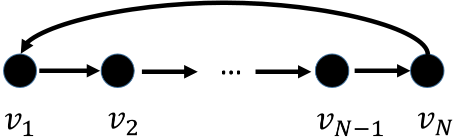
Figure 1: Directed cycle graph.

III-A Graph Signal Processing

III-A1 Graph Signals

Let $\mathcal{G}=\mathcal{G}(A)=(\mathcal{V},\mathcal{E})$ be the graph corresponding to matrix $A\in\mathbb{C}^{N\times N}$, where $\mathcal{V}$ is the set of $N$ nodes and a nonzero entry $\left[A\right]_{ij}$ denotes a directed edge $e_{ij}\in\mathcal{E}$ from node $j$ to node $i$. In real-world applications, such nodes can be represented by geo-locations of a road network, and the edges can be specified by one-way or two-way streets. Define graph signal $s:\mathcal{V}\rightarrow\mathcal{S}$ on $\mathcal{G}$, where $\mathcal{S}$ represents the signal space over the nodes of $\mathcal{G}$. We take $\mathcal{S}=\mathbb{C}^{N}$ such that $s=(s_{1},\dots,s_{N})\in\mathbb{C}^{N}$ and $s_{i}$ represents a measure at node $v_{i}\in\mathcal{V}$. In real-world applications, such signals can be specified by sensor measurements or datasets.

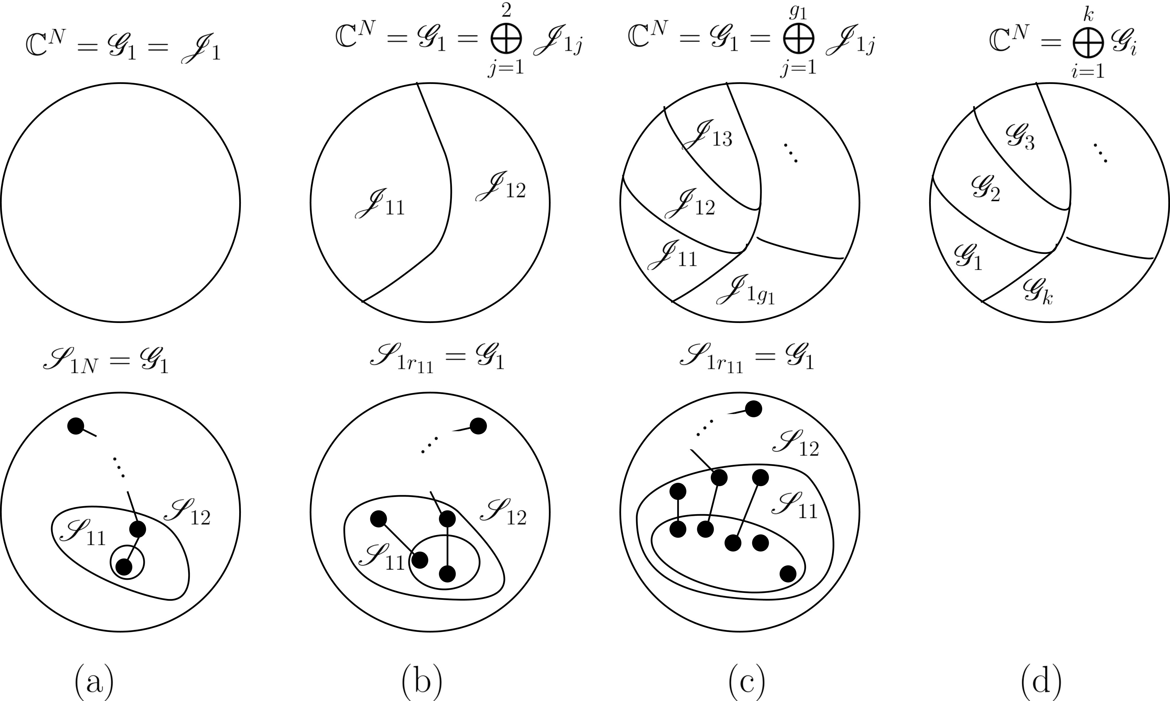
Figure 2: Illustration of generalized eigenspace partitions and Jordan chains of adjacency matrix $A\in\mathbb{C}^{N\times N}$ for (a) a single Jordan block, (b) one eigenvalue and two Jordan blocks, (c) one eigenvalue and multiple Jordan blocks, and (d) multiple eigenvalues. In (a)-(c) (bottom), each point represents a vector in a Jordan chain of $A$; points connected by lines illustrate a single Jordan chain. The partial multiplicities depicted for $\lambda_{1}$ are (a) $N$, (b) $r_{11}=N-2$ and $2$, and (c) $r_{11}=N-6$, $2$, $2$, $1$, and $1$. Each generalized eigenspace $\mathscr{G}_{i}$ in (d) can be visualized by (a)-(c).

III-A2 Graph Shift

As in [1, 3], the graph shift is the graph signal processing counterpart to the shift operator $z^{-1}$ in digital signal processing. The graph shift is defined as the operator that replaces the element $s_{i}$ of graph signal $s=(s_{1},\dots,s_{N})$ corresponding to node $v_{i}\in V$ with the linear combination of the signal elements at its in-neighbors (nodes $v_{k}\in V$ that participate in an edge $e_{ik}\in\mathcal{E}$), denoted by set $\mathcal{N}_{i}$; i.e., the shifted signal has elements $\widetilde{s}_{i}=\sum_{v_{j}\in\mathcal{N}_{i}}\left[A\right]_{ij}s_{j}$, or

$$\widetilde{s}=As.$$ (2)

Consistency with discrete signal processing can be seen by considering the directed cycle graph in Figure 1, which represents a finite, periodic time-series signal. The adjacency matrix of the graph is circulant matrix (elements not shown are zero)

$$C=\begin{bmatrix}&&&&&1\\ 1\\ &&\ddots\\ &&&&1\end{bmatrix}.$$ (3)

The shift $\widetilde{s}=Cs$ yields the time delay $\widetilde{s}_{i}=s_{i-1\,\,\mathrm{mod}\,N}$.

Reference [1] shows that the graph shift motivates defining the graph Fourier transform as the signal projection onto the eigenvectors of $A$. Our transform in Section IV builds on this concept to develop a framework to handle defective adjacency matrices.

III-A3 Graph Filter

The graph shift is a simple graph filter, where a graph filter $\mathbf{H}\in\mathbb{C}^{N\times N}$ represents a (linear) system with output $\mathbf{H}s$ for any graph signal $s\in\mathcal{S}$. As shown in Theorem 1 of [1], graph filter $\mathbf{H}$ is shift-invariant, or

$$A\left(\mathbf{H}\right)s=\mathbf{H}\left(As\right),$$ (4)

if and only if a polynomial $h(x)=\sum_{i=0}^{L}h_{i}x^{i}$ exists for constants $h_{0},h_{1},\dots,h_{L}\in\mathbb{C}$ such that $\mathbf{H}=h(A)=\sum_{i=0}^{L}h_{i}A^{i}$. This condition holds whenever the characteristic and minimal polynomials of $A$ are equal [1].

For defective $A$ with unequal characteristic and minimal polynomials such as the examples seen in this paper, shift-invariance cannot be claimed; however, an equivalent graph filter can be designed in terms of a matrix that is the image of a polynomial of $A$ [1]. The properties of such graph filters are established in [1].

III-B Eigendecomposition

This section and Appendix A provide a review of Jordan decompositions. The reader is directed to [28, 29, 32, 33] for additional background. Jordan subspaces and the Jordan decomposition are defined in this section.

The generalized eigenspaces $\mathscr{G}_{i}=\mathrm{Ker}(A-\lambda_{i}I)^{m_{i}}$ of $A\in\mathbb{C}^{N\times N}$ corresponding to its $k$ distinct eigenvalues $\lambda_{i}$ decompose $\mathbb{C}^{N}$ in terms of the direct sum

$$\mathbb{C}^{N}=\bigoplus_{i=1}^{k}\mathscr{G}_{i}$$ (5)

as depicted in Figure 2d; see also Appendix A.

Let $v_{1}\in\mathrm{Ker}(A-\lambda_{i}I)$, $v_{1}\neq 0$, be one of the $g_{i}$ proper eigenvectors of $A$ corresponding to the eigenvalue $\lambda_{i}$. It generates by recursion the generalized eigenvectors

$$Av_{p}=\lambda_{i}v_{p}+v_{p-1},\>\>p=2,\dots,r$$ (6)

where $r$ is the minimal positive integer such that $\left(A-\lambda_{i}I\right)^{r}v_{r}=0$ and $\left(A-\lambda_{i}I\right)^{r-1}v_{r}\neq 0$. Such a sequence of vectors $(v_{1},\dots,v_{r})$ that satisfies (6) is a Jordan chain of length $r$. The Jordan chain vectors are linearly independent and span a Jordan subspace, or,

$$\mathscr{J}=\mathrm{span}\left(v_{1},v_{2},\dots,v_{r}\right).$$ (7)

Order the Jordan subspaces of $\lambda_{i}$ by decreasing dimension and denote by $\mathscr{J}_{ij}$ the $j$th Jordan subspace of $\lambda_{i}$ with dimension $r_{ij}\leq m_{i}$, where $\{r_{ij}\}_{j=1}^{g_{i}}$ are called the partial multiplicities of $\lambda_{i}$. Then the generalized eigenspace $\mathscr{G}_{i}=\mathrm{Ker}(A-\lambda I)^{m_{i}}$ of $\lambda_{i}$ can be decomposed as

$$\mathscr{G}_{i}=\bigoplus_{j=1}^{g_{i}}\mathscr{J}_{ij}$$ (8)

as depicted in Figures 2a-c. Combining (8) and (5), the Jordan subspaces uniquely decompose $\mathbb{C}^{N}$ as

$$\mathbb{C}^{N}=\bigoplus_{i=1}^{k}\bigoplus_{j=1}^{g_{i}}\mathscr{J}_{ij}.$$ (9)

Furthermore, the cyclic Jordan subspaces cannot be represented as direct sums of smaller invariant subspaces; that is, the Jordan subspaces are irreducible components of $\mathbb{C}^{N}$ (see, e.g., p. 318 of [32]).

Figure 2 illustrates possible Jordan subspace structures of $A$, with the top row showing the tessellation of vector space $\mathbb{C}^{N}$ by the generalized or root eigenspace $\mathscr{G}_{i}=\mathrm{Ker}\left(A-\lambda_{i}I\right)^{m_{i}}$ and by the Jordan spaces $\mathscr{J}_{ij}$, and the bottom row illustrating the telescoping of $\mathbb{C}^{N}$ by the generalized eigenspaces of order $p$. Figure 2a illustrates $\mathbb{C}^{N}$ for a matrix with a single Jordan chain, represented by connected points in $\mathbb{C}^{N}$. The case of a matrix with two Jordan blocks corresponding to one eigenvalue is shown in Figure 2b. Figure 2c shows $\mathbb{C}^{N}$ for a matrix with a single eigenvalue and multiple Jordan blocks, and Figure 2d depicts the tessellation of the space in terms of the generalized eigenspaces for the case of multiple distinct eigenvalues.

Jordan decomposition. Appendix A defines eigenvector matrix $V$ and Jordan normal form $J$ such that $A=VJV^{-1}$. An important property of this decomposition is that Jordan chains are not unique and not necessarily orthogonal. For example, the $3\times 3$ matrix

$$A=\begin{bmatrix}0&1&1\\ 0&0&1\\ 0&0&0\end{bmatrix}$$ (10)

can have distinct eigenvector matrices

$$V_{1}=\left[\begin{array}[]{lrr}1&-1&1\\ 0&1&-2\\ 0&0&1\end{array}\right],V_{2}=\left[\begin{array}[]{lrr}1&0&0\\ 0&1&-1\\ 0&0&1\end{array}\right],$$ (11)

where the Jordan chain vectors are the columns of $V_{1}$ and $V_{2}$ and so satisfy (6). Since Jordan chains are not unique, the Jordan subspace is used in Section IV to characterize the possible generalized eigenvectors.

IV Spectral Projector-Based Graph Signal Processing

This section presents a basis-invariant coordinate free graph Fourier transform with respect to a set of known proper eigenvectors. For graphs with diagonalizable adjacency matrices, the coordinate form of this transform resolves with appropriate choice of basis vectors to that of [1, 3]. The interpretation of the spectral components is settled for the cases of repeated eigenvalues and non-diagonalizable, or defective, adjacency matrices.

Consider matrix $A$ with distinct eigenvalues $\lambda_{1},\dots,\lambda_{k}$, $k\leq N$, that has Jordan decomposition $A=VJV^{-1}$. Denote by $\mathscr{J}_{ij}$ the $j$th Jordan subspace of dimension $r_{ij}$ corresponding to eigenvalue $\lambda_{i}$, $i=1,\dots,k$, $j=1,\dots,g_{i}$. Each $\mathscr{J}_{ij}$ is $A$-invariant and irreducible (see Section III-B). Then, the Jordan subspaces are the spectral components of the signal space $\mathcal{S}=\mathbb{C}^{N}$ and define the graph Fourier transform of a graph signal $s\in\mathcal{S}$ as the mapping

$$\mathcal{F}:\mathcal{S} \rightarrow\bigoplus_{i=1}^{k}\bigoplus_{j=1}^{g_{i}}\mathscr{J}_{ij}$$

$$s \rightarrow\left(\widehat{s}_{11},\dots,\widehat{s}_{1g_{1}},\dots,\widehat{s}_{k1},\dots,\widehat{s}_{kg_{k}}\right).$$ (12)

That is, the Fourier transform of $s$, is the unique decomposition

$$s=\sum_{i=1}^{k}\sum_{j=1}^{g_{i}}\widehat{s}_{ij},\hskip 28.45274pt\widehat{s}_{ij}\in\mathscr{J}_{ij}.$$ (13)

The distinct eigenvalues $\lambda_{1},\dots,\lambda_{k}$ are the graph frequencies of graph $\mathcal{G}(A)$. The frequency or spectral components of graph frequency $\lambda_{i}$ are the Jordan subspaces $\mathscr{J}_{ij}$. The total number of frequency components corresponding to $\lambda_{i}$ is its geometric multiplicity $g_{i}$. In this way, when $g_{i}>1$, frequency $\lambda_{i}$ corresponds to more than one frequency component.

To highlight the significance of (12) and (13), consider the signal expansion of a graph signal $s$ with respect to graph $\mathcal{G}(A)$:

$$s=\widetilde{s}_{1}v_{1}+\cdots+\widetilde{s}_{N}v_{N}=V\widetilde{s},$$ (14)

where $v_{i}$ is the $i$th basis vector in a Jordan basis of $A$, $V$ is the corresponding eigenvector matrix, and $\widetilde{s}_{i}$ is the $i$th expansion coefficient. As discussed in Section III-B, the choice of Jordan basis has degrees of freedom when the dimension of a cyclic Jordan subspace is greater than one. Therefore, if $\mathrm{dim}\mathscr{J}_{ij}\geq 2$, there exists eigenvector submatrix $X_{ij}\neq V_{ij}$ such that $\mathrm{span}\{X_{ij}\}=\mathrm{span}\{V_{ij}\}=\mathscr{J}_{ij}$. Thus, the signal expansion (14) is not unique when $A$ has Jordan subspaces of dimension $r>1$.

In contrast, the Fourier transform given by (12) and (13) yields a unique signal expansion that is independent of the choice of Jordan basis. Given any Jordan basis $v_{1},\dots,v_{N}$ with respect to $A$, the $j$th spectral component of eigenvalue $\lambda_{i}$ is, by (13), $\widehat{s}_{ij}=\sum_{k=p}^{p+r_{ij}-1}\widetilde{s}_{k}v_{k}$, where $v_{p},\dots,v_{p+r_{ij}-1}$ are a basis of $\mathscr{J}_{ij}$. Under this definition, there is no ambiguity in the interpretation of frequency components even when Jordan subspaces have dimension $r>1$ or there are repeated eigenvalues. The properties of the spectral components are discussed in more detail below.

IV-A Spectral Components

The spectral components of the Fourier transform (12) are expressed in terms of basis $v_{1},\dots,v_{N}$ and its dual basis $w_{1},\dots,w_{N}$ since the chosen Jordan basis may not be orthogonal. Denote the basis and dual basis matrices by $V=[v_{1}\cdots v_{N}]$ and $W=[w_{1}\cdots,w_{N}]$. By definition, $\langle w_{i},v_{j}\rangle=w_{i}^{H}v_{j}=\delta_{ij}$, where $\delta_{ij}$ is the Kronecker delta function [33, 34]. Then $W^{H}V=V^{H}W=I$, so the dual basis is the inverse Hermitian $W=V^{-H}$ and correspond to the left eigenbasis.

Partition Jordan basis matrix $V$ as (58) so that each $V_{ij}\in\mathbb{C}^{N\times r_{ij}}$ spans Jordan subspace $\mathscr{J}_{ij}$. Similarly, partition the dual basis matrix by rows as $W=[\cdots W_{i1}^{H}\cdots W_{ig_{i}}^{H}\cdots]^{T}$, with each $W_{ij}^{H}\in\mathbb{C}^{r_{ij}\times N}$. Suppose $V_{ij}=[v_{1}\cdots v_{r_{ij}}]$ with corresponding coefficients $\widetilde{s}_{1},\dots,\widetilde{s}_{r_{ij}}$ in the Jordan basis expansion (14). Define an $N\times N$ matrix $V^{0}_{ij}=[0\cdots V_{ij}\cdots 0]$ that is zero except for the columns corresponding to $V_{ij}$. Then each spectral component corresponding to Jordan subspace $\mathscr{J}_{ij}$ can be written as (below, diagonal dots and elements not shown are zero)

$$\widehat{s}_{ij} =\widetilde{s}_{1}v_{1}+\dots+\widetilde{s}_{r_{ij}}v_{r_{ij}}$$ (15)

$$=V^{0}_{ij}\widetilde{s}$$ (16)

$$=V_{ij}^{0}V^{-1}s$$ (17)

$$=V\begin{bmatrix}\ddots\\ &I_{r_{ij}}\\ &&\ddots\end{bmatrix}V^{-1}s$$ (18)

$$=V\begin{bmatrix}\ddots\\ &I_{r_{ij}}\\ &&\ddots\end{bmatrix}W^{H}s$$ (19)

$$=V_{ij}W^{H}_{ij}s,$$ (20)

for $i=1,\dots,k$ and $j=1,\dots,g_{i}$. Denote

$$P_{ij}=V_{ij}W^{H}_{ij},$$ (21)

which is the projection matrix onto $\mathcal{S}_{ij}$ parallel to complementary subspace $\mathcal{S}\setminus\mathcal{S}_{ij}$. Note that $P_{ij}^{2}=V_{ij}W^{H}_{ij}V_{ij}W^{H}_{ij}=V_{ij}W^{H}_{ij}=P_{ij}$.

The projection matrices $\{P_{ij}\}_{j=1}^{r_{ij}}$ are related to the first component matrix $Z_{i0}$ of eigenvalue $\lambda_{i}$. The component matrix is defined as [28, Section 9.5]

$$Z_{i0}=V\begin{bmatrix}\ddots\\ &I_{a_{i}}\\ &&\ddots\end{bmatrix}V^{-1}$$ (22)

where $a_{i}=\sum_{j=1}^{g_{i}}r_{ij}$ is the algebraic multiplicity of $\lambda_{i}$. This matrix acts as a projection matrix onto the generalized eigenspace.

Theorem 1 provides additional properties of projection matrix $P_{ij}$.

Theorem 1.

For matrix $A\in\mathbb{C}^{N\times N}$ with eigenvalues $\lambda_{1},\dots,\lambda_{k}$, the projection matrices $P_{ij}$ onto the $j$th Jordan subspace $\mathscr{J}_{ij}$ corresponding to eigenvalue $\lambda_{i}$, $i=1,\dots,k$, $j=1,\dots,g_{i}$, satisfy the following properties:

1. $P_{ij}P_{kl}=\delta_{ik}\delta_{jl}P_{ij}$, where $\delta$ is the Kronecker delta function;

2. $\sum_{j=1}^{g_{i}}P_{ij}=Z_{i0}$, where $Z_{i0}$ is the component matrix of eigenvalue $\lambda_{i}$;

Proof:

(a) Since $W^{H}V=I$, the partition of $W^{H}$ and $V$ that yields (20) satisfies $W^{H}_{ij}V_{kl}=\delta_{ik}\delta_{jl}I_{r_{ij}\times r_{kl}}$, where $r_{ij}$ is the dimension of the Jordan subspace corresponding to $P_{ij}$, $r_{kl}$ the dimension of Jordan subspace corresponding to $P_{kl}$, and matrix $I_{r_{ij}\times r_{kl}}$ consists of the first $r_{kl}$ canonical vectors $e_{i}=(0,\dots,1,\dots,0)$, where $1$ is at the $i$th index. Then it follows that

$$P_{ij}P_{kl} =V_{ij}W^{H}_{ij}V_{kl}W^{H}_{kl}$$ (23)

$$=V_{ij}\left(\delta_{ik}\delta_{jl}I_{r_{ij}\times r_{kl}}\right)W^{H}_{kl}.$$ (24)

If $i=k$ and $j=l$, then $P_{ij}P_{kl}=V_{ij}I_{r_{ij}\times r_{ij}}W^{H}_{ij}=P_{ij}$; otherwise, $P_{ij}P_{kl}=0$.

(b) Write

$$\sum_{j=1}^{g_{i}}P_{ij} =\sum_{j=1}^{g_{i}}V\begin{bmatrix}\ddots\\ &I_{r_{ij}}\\ &&\ddots\end{bmatrix}V^{-1}$$ (25)

$$=V\left(\sum_{j=1}^{g_{i}}\begin{bmatrix}\ddots\\ &I_{r_{ij}}\\ &&\ddots\end{bmatrix}\right)V^{-1}$$ (26)

$$=V\begin{bmatrix}\ddots\\ &I_{\sum\limits_{j=1}^{g_{i}}r_{ij}}\\ &&\ddots\end{bmatrix}V^{-1}$$ (27)

$$=Z_{i0},$$ (28)

or the first component matrix of $A$ for eigenvalue $\lambda_{i}$. ∎

Theorem 1(a) shows that each projection matrix $P_{ij}$ only projects onto Jordan subspace $\mathscr{J}_{ij}$. Theorem 1(b) shows that the sum of projection matrices for a given eigenvalue equals the component matrix of that eigenvalue.

This section provides the mathematical foundation for a graph Fourier transform based on projections onto the Jordan subspace of an adjacency matrix. The next section motivates ranking signal projections on Jordan subspaces by the energy of the signal projections.

V Generalized Parseval’s Identity

As discussed above, a chosen Jordan basis for matrix $A\in\mathbb{C}^{N\times N}$, represented by the eigenvector matrix $V$, may not be orthogonal. Therefore, Parseval’s identity may not hold. Nevertheless, a generalized Parseval’s identity does exist in terms of the Jordan basis and its dual; see also [34]. For a dual basis matrix $W=V^{-H}$, the following property holds:

Property 2 (Generalized Parseval’s Identity).

Consider graph signals $s_{1},s_{2}\in\mathbb{C}^{N}$ over graph $\mathcal{G}(A)$, $A\in\mathbb{C}^{N\times N}$. Let $V=[v_{1}\cdots v_{N}]$ be a Jordan basis for $A$ with dual basis $W=V^{-H}$ partitioned as $[w_{1}\cdots w_{N}]$. Let $s=\sum_{i=1}^{N}\langle s,v_{i}\rangle v_{i}=V\widetilde{s}_{V}$ be the representation of $s$ in basis $V$ and $s=\sum_{i=1}^{N}\langle s,w_{i}\rangle w_{i}=W\widetilde{s}_{W}$ be the representation of $s$ in basis $W$. Then

$$\langle s_{1},s_{2}\rangle=\langle\widetilde{s}_{1,V},\widetilde{s}_{2,W}\rangle.$$ (29)

By extension,

$$\left\|s\right\|^{2}=\langle s,s\rangle=\langle\widetilde{s}_{V},\widetilde{s}_{W}\rangle.$$ (30)

Equations (29) and (30) hold regardless of the choice of eigenvector basis.

Energy of spectral components. The energy of a discrete signal $s\in\mathbb{C}^{N}$ is defined as [35, 36]

$$E_{s}=\langle s,s\rangle=\left\|s\right\|^{2}=\sum_{i=1}^{N}\left|s\right|^{2}.$$ (31)

Equation (30) thus illustrates conservation of signal energy in terms of both a Jordan basis and its dual.

The energy of the signal projections onto the spectral components of $\mathcal{G}(A)$ for the GFT (12) is next defined. Write $\widehat{s}_{i,j}$ in terms of the columns of $V$ as $\widehat{s}_{i,j}=\alpha_{1}v_{i,j,1}+\dots\alpha_{r_{ij}}v_{i,j,r_{ij}}$ and in terms of the columns of $W$ as $\widehat{s}_{i,j}=\beta_{1}w_{i,j,1}+\dots\beta_{r_{ij}}w_{i,j,r_{ij}}$. Then the energy of $\widehat{s}_{ij}$ can be defined as

$$\|\widehat{s}_{ij}\|^{2}=\langle\alpha,\beta\rangle$$ (32)

using the notation $\alpha=(\alpha_{1},\dots,\alpha_{r_{ij}})$ and $\beta=(\beta_{1},\dots,\beta_{r_{ij}})$.

The generalized Parseval’s identity expresses the energy of the signal in terms of the signal expansion coefficients $\widetilde{s}$, which highlights the importance of choosing a Jordan basis. This emphasizes that both the GFT $\{\widehat{s}_{ij}\}$ and the signal expansion coefficients $\widetilde{s}$ are necessary to fully characterize the graph Fourier domain.

Normal $A$. When $A$ is normal (i.e., when $AA^{H}=A^{H}A$), $V$ can be chosen to have unitary columns. Then, $V=W$ so

$$\langle s_{1},s_{2}\rangle=\langle\widetilde{s}_{1},\widetilde{s}_{2}\rangle$$ (33)

and

$$\left\|s\right\|^{2}=\langle s,s\rangle=\left\|\widetilde{s}\right\|^{2}.$$ (34)

Note that (33) and (34) do not hold in general for diagonalizable $A$.

While the Jordan basis, or choice of eigenvectors, is not unique, the image of a signal $s$ under the projection matrix $P_{ij}$ (21) is invariant to the choice of Jordan basis. This section shows that these projections can be ranked in terms of the percentage of recovered signal energy.

The next section demonstrates a total variation-based ranking of the spectral components.

VI Total Variation Ordering

This section defines a mapping of spectral components to the real line to achieve an ordering of the spectral components. This ordering can be used to distinguish generalized low and high frequencies as in [3]. An upper bound for a total-variation based mapping of a spectral component (Jordan subspace) is derived.

As in [3, 37], the total variation for finite discrete-valued (periodic) time series $s$ is defined as

$$\mathrm{TV}\left(s\right)=\sum_{n=0}^{N-1}\left|s_{n}-s_{n-1\,\,\mathrm{mod}N}\right|=\left\|s-Cs\right\|_{1},$$ (35)

where $C$ is the circulant matrix (3) that represents the DSP shift operator. As in [3], (35) is generalized to the graph shift $A$ to define the graph total variation

$$\mathrm{TV}_{G}\left(s\right)=\left\|s-As\right\|_{1}.$$ (36)

Matrix $A$ can be replaced by $A^{\mathrm{norm}}=\frac{1}{\left|\lambda_{\mathrm{max}}\right|}A$ when the maximum eigenvalue satisfies $|\lambda_{\mathrm{max}}|>0$.

Equation (36) can be applied to define the total variation of a spectral component. These components are the cyclic Jordan subspaces of the graph shift $A$ as described in Section III-B. Choose a Jordan basis of $A$ so that $V$ is the eigenvector matrix of $A$, i.e., $A=VJV^{-1}$, where $J$ is the Jordan form of $A$. Partition $V$ into $N\times r_{ij}$ submatrices $V_{ij}$ whose columns are a Jordan chain of (and thus span) the $j$th Jordan subspace $\mathscr{J}_{ij}$ of eigenvalue $\lambda_{i}$, $i=1,\dots,k\leq N$, $j=1,\dots,g_{i}$. Define the (graph) total variation of $V_{ij}$ as

$$\mathrm{TV}_{G}\left(V_{ij}\right)=\left\|V_{ij}-AV_{ij}\right\|_{1},$$ (37)

where $\|\cdot\|_{1}$ represents the induced L1 matrix norm (equal to the maximum absolute column sum).

The next theorem shows equivalent formulations for the graph total variation (37).

Theorem 3.

The graph total variation with respect to GFT (12) can be written as

$$\mathrm{TV}_{G}\left(V_{ij}\right)=\left\|V_{ij}\left(I_{r_{ij}}-J_{ij}\right)\right\|_{1}$$ (38)

$$=\max_{i=2,\dots,r_{ij}}\left\{\left|1-\lambda\right|\left\|v_{1}\right\|_{1},\left\|\left(1-\lambda\right)v_{i}-v_{i-1}\right\|_{1}\right\}.$$ (39)

Proof:

Simplify (37) to obtain

$$\mathrm{TV}_{G}\left(V_{ij}\right) =\left\|V_{ij}-VJV^{-1}V_{ij}\right\|_{1}$$ (40)

$$=\left\|V_{ij}-VJ\begin{bmatrix}\underline{0}\\ I_{r_{ij}}\\ \underline{0}\end{bmatrix}\right\|_{1}$$ (41)

$$=\left\|V_{ij}-V\begin{bmatrix}\underline{0}\\ &J_{ij}\\ &&\underline{0}\end{bmatrix}\right\|_{1}$$ (42)

$$=\left\|V_{ij}-V_{ij}J_{ij}\right\|_{1}$$ (43)

$$=\left\|V_{ij}\left(I_{r_{ij}}-J_{ij}\right)\right\|_{1}.$$ (44)

Let $\lambda$ denote the $i$th eigenvalue and the columns $v_{1},\dots,v_{r_{ij}}$ of $V_{ij}$ comprise its $j$th Jordan chain. Then (38) can be expressed in terms of the Jordan chain:

$$\mathrm{TV}_{G}\left(V_{ij}\right)$$ (45)

$$=\left\|\begin{bmatrix}v_{1}\dots v_{r_{ij}}\end{bmatrix}\begin{bmatrix}1-\lambda&-1\\ &1-\lambda&\ddots\\ &&\ddots&-1\\ &&&1-\lambda\end{bmatrix}\right\|_{1}$$ (46)

$$=\left\|\begin{bmatrix}\left(1-\lambda\right)v_{1}&\left(1-\lambda\right)v_{2}-v_{1}&\cdots&\end{bmatrix}\right\|_{1}$$ (47)

$$=\max_{i=2,\dots,r_{ij}}\left\{\left|1-\lambda\right|\left\|v_{1}\right\|_{1},\left\|\left(1-\lambda\right)v_{i}-v_{i-1}\right\|_{1}\right\}.$$ (48)

∎

Theorem 4 shows that $V$ can be chosen such that $\left\|V_{ij}\right\|_{1}=1$ without loss of generality.

Theorem 4.

The eigenvector matrix $V$ of adjacency matrix $A\in\mathbb{C}^{N\times N}$ can be chosen so that each Jordan chain represented by the eigenvector submatrix $V_{ij}\in\mathbb{C}^{N\times r_{ij}}$ satisfies $\left\|V_{ij}\right\|_{1}=1$; i.e., $\left\|V\right\|_{1}=1$ without loss of generality.

Proof:

Let $V$ represent an eigenvector matrix of $A$ with partitions $V_{ij}$ as described above, and let $J_{ij}$ represent the corresponding Jordan block. Let $D$ be a block diagonal matrix with $r_{ij}\times r_{ij}$ diagonal blocks $D_{ij}=(1/\left\|V_{ij}\right\|_{1})I_{r_{ij}}$. Since $D_{ij}$ commutes with $J_{ij}$, $D$ commutes with $J$. Note that $D$ is a special case of upper triangular Toeplitz matrices discussed in [28, Example 6.5.4, Theorem 12.4.1].

Let $X=VD$ and $B=XJX^{-1}$. Then

$$B =XJX^{-1}$$ (49)

$$=VDJD^{-1}V^{-1}$$ (50)

$$=VDD^{-1}JV^{-1}$$ (51)

$$=VJV^{-1}$$ (52)

$$=A.$$ (53)

Therefore, both $V$ and $X$ are eigenvector matrices of $A$. ∎

In the following, it is assumed that $V$ satisfies Theorem 4. Theorem 5 presents an upper bound of (38).

Theorem 5.

Consider matrix $A$ with $k$ distinct eigenvalues and $N\times r_{ij}$ matrices $V_{ij}$ with columns comprising the $j$th Jordan chain of $\lambda_{i}$, $i=1,\dots,k$, $j=1,\dots,g_{i}$. Then the graph total variation $\mathrm{TV}_{G}(V_{ij})\leq\left|1-\lambda_{i}\right|+1$.

Proof:

Let $\left\|V_{ij}\right\|_{1}=1$ and rewrite (38):

$$\mathrm{TV}_{G}\left(V_{ij}\right) \leq\left\|V_{ij}\right\|_{1}\left\|I_{r_{ij}}-J_{ij}\right\|_{1}$$ (54)

$$=\left\|I_{r_{ij}}-J_{ij}\right\|_{1}$$ (55)

$$=\left|1-\lambda_{i}\right|+1.$$ (56)

∎

Equations (38), (39), and (56) characterize the (graph) total variation of a Jordan chain by quantifying the change in a set of vectors that spans the Jordan subspace $\mathscr{J}_{ij}$ when they are transformed by the graph shift $A$. While this total variation bound may not capture the true total variation of a spectral component, it can be generalized as an upper bound for all spectral components associated with a Jordan equivalence class. This concept is explored further in [31].

(a) Average number of June-August trips, Fridays 9pm-10pm

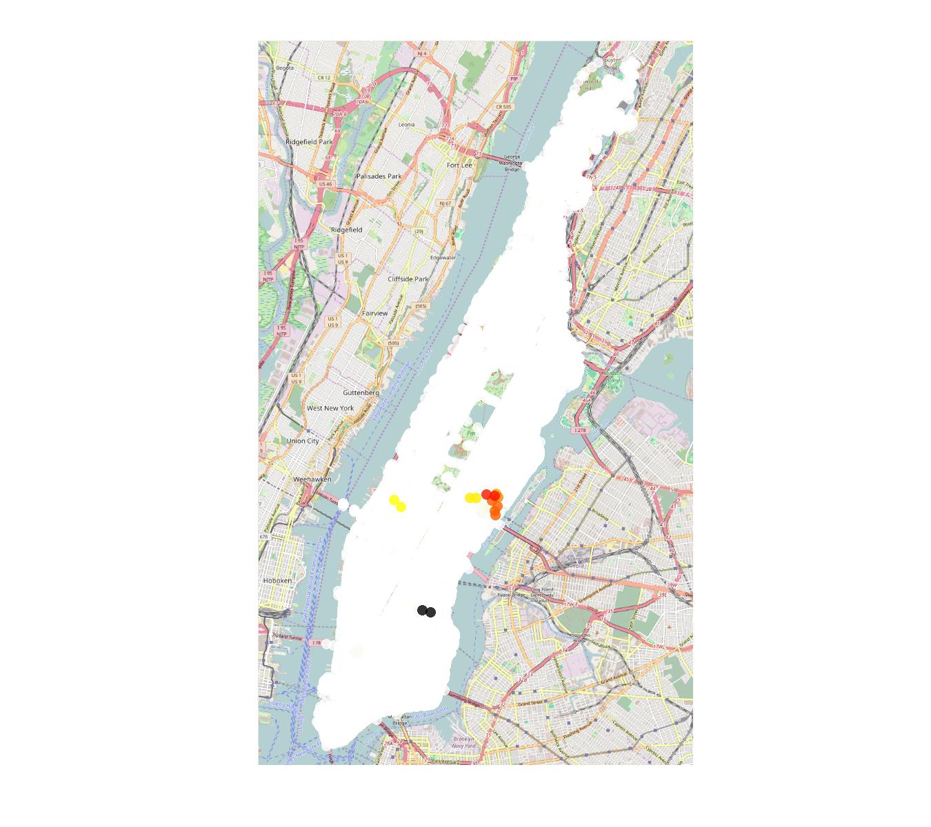
(b) Maximum expressed eigenvector

Figure 3: Graph signal based on NYC taxi data (a) and the maximum expressed eigenvector (b). (a) Colors denote log₁₀ bins of the four-year average number of trips for Fridays 9pm-10pm (699 log bins; white: 0–20, beige to yellow: 20–230, orange: 230–400, red: 400–550, blue: 550–610, purple to black: 610–2,700. (b) All colors except white indicate locations with a concentrated number of taxi trips. Black indicates the locations of maximum expression in the eigenvector. The plots were generated with ggmap [38] and OpenStreetMap [39].

VII Application

We apply the graph Fourier transform (12) to a signal based on 2010-2013 New York City taxi data [40] over the Manhattan road network. The signal represents the four-year average number of trips that pass through each node of the road network as determined by Dijkstra path estimates from the start- and end-coordinates (latitude and longitude) provided by the raw data; the computation behind these estimates is described in [41]. The road network consists of 6,408 nodes that represent latitude and longitude coordinates from [42] that are connected by 14,418 directed edges that represent one-way directions as verified by Google Maps [43]. The adjacency matrix of the road network is defective with 253 Jordan chains of length 2 and 193 eigenvectors without Jordan chain vectors corresponding to eigenvalue zero (446 Jordan chains total). Details for the eigendecomposition of this matrix are described in [44, 30].

Figure 3(a) shows the signal, consisting of the four-year June-August average number of trips at each node of the Manhattan road network for Fridays 9pm-10pm. Applying the GFT (12) and computing the energies of the signal projections as described in Section V yields a highly expressed eigenvector shown in Figure 3(b). This eigenvector shows that most of the signal energy is concentrated at Gramercy Park (shown in black), north of Gramercy Park, and in Hell’s Kitchen on the west side of Manhattan.

VIII Limitations

The graph Fourier transform presented in this paper solves the problem of uniqueness for defective adjacency matrices by projecting a signal onto Jordan subspaces instead of eigenvectors and generalized eigenvectors. This method relies on Jordan chain computations, however, which is sensitive to numerical errors and can be expensive when the number of chains to compute and the graph dimension are large and the computing infrastructure is memory-bound. The computation can be accelerated by using equivalence classes over graph topologies, as we discuss in [31]. These classes allow matching between a given graph to graphs of simpler topologies such that the graph Fourier transform of a signal with respect to these graphs is preserver. Since the equivalence classes may not be applicable to arbitrary graph structures, we explore inexact eigendecomposition methods in [30] to reduce the execution time and bypass the numerically unstable Jordan chain computation.

IX Conclusion

The graph Fourier transform proposed here provides a unique and non-ambiguous spectral decomposition for signals over graphs with defective, or non-diagonalizable, adjacency matrices. The transform is based on spectral projections of signals onto the Jordan subspaces of the graph adjacency matrix. This coordinate free graph Fourier transform is unique and leads to a unique spectral decomposition of graph signals. This paper shows that the signal projections onto the Jordan subspaces can be ranked by energy via a generalized Parseval’s identity. Lastly, a total variation-based ordering of the Jordan subspaces is proposed. This allows ordering frequencies, and to define low-, high-, and band-pass graph signals.

Appendix A Background on Jordan Decompositions

Direct sum. Let $X_{1},\dots,X_{k}$ be subspaces of vector space $X$ such that $X=X_{1}+\cdots+X_{k}$. If $X_{i}\cap X_{j}=\emptyset$ for all $i\neq j$, then $X$ is the direct sum of subspaces $\{X_{i}\}_{i=1}^{k}$, denoted as $X=\bigoplus_{i=1}^{k}X_{i}$. Any $x\in X$ can be written uniquely as $x=x_{1}+\cdots+x_{k}$, where $x_{i}\in X_{i}$, $i=1,\dots,k$.

Eigenvalues and multiplicities. Consider matrix $A\in\mathbb{C}^{N\times N}$ with $k$ distinct eigenvalues $\lambda_{1},\dots,\lambda_{k}$, $k\leq N$. The eigenvalues of $A$ are the roots of the characteristic polynomial $\varphi_{A}(\lambda)=\det(A-\lambda I)=\prod_{i=1}^{k}\left(\lambda-\lambda_{i}\right)^{a_{i}}$, $I$ is the identity matrix, and exponent $a_{i}$ represents the algebraic multiplicity of eigenvalue $\lambda_{i}$, $i=1,\dots,k$. Denote by $\mathrm{Ker}(A)$ the kernel or null space of matrix $A$, i.e., the span of vectors $v$ satisfying $Av=0$. The geometric multiplicity $g_{i}$ of eigenvalue $\lambda_{i}$ equals the dimension of null space $\mathrm{Ker}\left(A-\lambda_{i}I\right)$. The minimal polynomial $m_{A}(\lambda)$ of $A$ has form $m_{A}(\lambda)=\prod_{i=1}^{k}\left(\lambda-\lambda_{i}\right)^{m_{i}}$, where $m_{i}$ is the index of eigenvalue $\lambda_{i}$. The index $m_{i}$ represents the maximum Jordan chain length or Jordan subspace dimension, which is discussed in more detail below.

Generalized eigenspaces. The eigenvectors and generalized eigenvectors of matrix $A\in\mathbb{C}^{N\times N}$ partition $\mathbb{C}^{N}$ into subspaces, some of which are spans of eigenvectors, eigenspaces, or generalized eigenspaces. Subspace $\mathscr{G}_{i}=\mathrm{Ker}\left(A-\lambda_{i}I\right)^{m_{i}}$ is the generalized eigenspace or root subspace of $\lambda_{i}$. The generalized eigenspaces are $A$-invariant; that is, for all $x\in\mathscr{G}_{i}$, $Ax\in\mathscr{G}_{i}$. The subspace $\mathscr{S}_{ip}=\mathrm{Ker}\left(A-\lambda_{i}I\right)^{p}$, $p=0,1,\dots,N$, is the generalized eigenspace of order $p$ for $\lambda_{i}$. For $p\geq m_{i}$, $\mathscr{S}_{ip}=\mathscr{G}_{i}$. The proper eigenvectors $v$ of $\lambda_{i}$, or simply eigenvectors of $\lambda_{i}$, are linearly independent vectors in $\mathscr{S}_{i1}=\mathrm{Ker}\left(A-\lambda_{i}I\right)$, the eigenspace of $\lambda_{i}$. There are $g_{i}=\mathrm{dim}\,\mathscr{S}_{i1}=\mathrm{dim}\,\mathrm{Ker}\left(A-\lambda_{i}I\right)$ eigenvectors of $\lambda_{i}$. Subspaces $\mathscr{S}_{ip}$ form a (maximal) chain of $\mathcal{G}_{i}$ as depicted in Figure 2; that is,

$$\{0\}\!=\!\mathscr{S}_{i0}\subset\mathscr{S}_{i1}\subset\!\cdots\subset\!\!\mathscr{S}_{i,m_{i}}=\mathscr{S}_{i,m_{i}+1}=\cdots\subset\mathbb{C}^{N}$$

where $m_{i}$ is the index of $\lambda_{i}$. Vectors $v\in\mathscr{S}_{ip}$ but $v\notin\mathscr{S}_{i,p-1}$ are generalized eigenvectors of order $p$ for $\lambda_{i}$.

Properties of Jordan subspaces. A Jordan subspace (7) is $A$-invariant; that is, for all $x\in\mathscr{J}$, $Ax\in\mathscr{J}$. The Jordan subspace $\mathscr{J}$ is also cyclic since it can be written by (6) as

$$\mathscr{J}=\mathrm{span}\left(v_{r},(A-\lambda I)v_{r},\dots,(A-\lambda I)^{r-1}v_{r}\right)$$ (57)

for $v_{r}\in\mathrm{Ker}(A-\lambda I)^{r}$, $v_{r}\neq 0$.

The number of Jordan subspaces corresponding to $\lambda_{i}$ equals the geometric multiplicity $g_{i}=\mathrm{dim}\,\mathrm{Ker}(A-\lambda I)$, since there are $g_{i}$ eigenvectors of $\lambda_{i}$. It can be shown that the Jordan spaces $\left\{\mathscr{J}_{ij}\right\}$, $j=1,\cdots,g_{i}$ and $i=1,\cdots,k$, are disjoint.

Jordan decomposition. Let $V_{ij}$ denote the $N\times r_{ij}$ matrix whose columns form a Jordan chain of eigenvalue $\lambda_{i}$ of $A$ that spans Jordan subspace $\mathscr{J}_{ij}$. Then the generalized eigenvector matrix $V$ of $A$ is

$$V=\begin{bmatrix}V_{11}\cdots V_{1g_{1}}&\cdots&V_{k1}\cdots V_{kg_{k}}\end{bmatrix},$$ (58)

where $k$ is the number of distinct eigenvalues. The columns of $V$ are a Jordan basis of $\mathbb{C}^{N}$. Then $A$ has block-diagonal Jordan normal form $J$ consisting of Jordan blocks

$$J(\lambda)=\begin{bmatrix}\lambda&1&\\ &\lambda&\ddots\\ &&\ddots&1\\ &&&\lambda\end{bmatrix}.$$ (59)

of size $r_{ij}$; see, for example, [28] or [45, p.125]. The Jordan normal form $J$ of $A$ is unique up to a permutation of the Jordan blocks. The Jordan decomposition of $A$ is $A=VJV^{-1}$.

References

- [1] A. Sandryhaila and J.M.F. Moura, “Discrete signal processing on graphs,” IEEE Transactions on Signal Processing, vol. 61, no. 7, pp. 1644–1656, Apr. 2013.
- [2] A. Sandryhaila and J.M.F. Moura, “Big data analysis with signal processing on graphs: Representation and processing of massive data sets with irregular structure,” IEEE Signal Processing Magazine, vol. 31, no. 5, pp. 80–90, Aug. 2014.
- [3] A. Sandryhaila and J.M.F. Moura, “Discrete signal processing on graphs: Frequency analysis,” IEEE Transactions on Signal Processing, vol. 62, no. 12, pp. 3042–3054, Jun. 2014.
- [4] D. Shuman, S.K. Narang, P. Frossard, A. Ortega, and P. Vandergheynst, “The emerging field of signal processing on graphs: Extending high-dimensional data analysis to networks and other irregular domains,” IEEE Signal Processing Magazine, vol. 30, no. 3, pp. 83–98, Apr. 2013.
- [5] M. Püschel and J.M.F. Moura, “Algebraic signal processing theory: Foundation and 1-d time,” IEEE Transactions on Signal Processing, vol. 56, no. 8, pp. 3572–3585, Aug. 2008.
- [6] M. Püschel and J.M.F. Moura, “Algebraic signal processing theory: 1-d space,” IEEE Transactions on Signal Processing, vol. 56, no. 8, pp. 3586–3599, Aug. 2008.
- [7] M. Püschel and J. M. F. Moura, “Algebraic signal processing theory: Cooley-Tukey type algorithms for DCTs and DSTs,” IEEE Transactions on Signal Processing, vol. 56, no. 4, pp. 1502–1521, April 2008.
- [8] K. Pearson, “On lines and planes of closest fit to systems of points in space,” Philosophical Magazine Series 6, vol. 2, no. 11, pp. 559–572, 1901.
- [9] H. Hotelling, “Analysis of a complex of statistical variables into principal components,” Journal of Educational Psychology, vol. 24, no. 6, pp. 417–441, 498––520, 1933.
- [10] H. Hotelling, “Relations between two sets of variates,” Biometrika, vol. 28, no. 3/4, pp. 321–377, 1936.
- [11] J. F. Tenenbaum, V. Silva, and J. C. Langford, “A global geometric framework for nonlinear dimensionality reduction,” Science, vol. 290, pp. 2319–2323, 2000.
- [12] S. Roweis and L. Saul, “Nonlinear dimensionality reduction by locally linear embedding,” Science, vol. 290, pp. 2323–2326, 2000.
- [13] M. Belkin and P. Niyogi, “Laplacian eigenmaps for dimensionality reduction and data representation,” Neural Computation, vol. 15, no. 6, pp. 1373–1396, 2003.
- [14] D. L. Donoho and C. Grimes, “Hessian eigenmaps: Locally linear embedding techniques for high-dimensional data,” Proceedings of the National Academy of Sciences, vol. 100, no. 10, pp. 5591–5596, 2003.
- [15] Mikhail Belkin and Partha Niyogi, “Towards a theoretical foundation for laplacian-based manifold methods,” Journal of Computer and System Sciences, vol. 74, no. 8, pp. 1289 – 1308, 2008.
- [16] D. Ganesan, B. Greenstein, D. Estrin, J. Heidemann, and R. Govindan, “Multiresolution storage and search in sensor networks,” ACM Transactions on Storage, vol. 1, pp. 277–315, 2005.
- [17] R. Wagner, H. Choi, R. Baraniuk, and V. Delouille, “Distributed wavelet transform for irregular sensor network grids,” in Proceedings of the 13th IEEE Workshop on Statistical Signal Processing, 2005, pp. 1196–1201.
- [18] R. Wagner, R. Baraniuk, S. Du, D. Johnson, and A. Cohen, “An architecture for distributed wavelet analysis and processing in sensor networks,” in Proceedings of the 5th ACM International Conference on Information Processing in Sensor Networks, 2006, pp. 243–250.
- [19] R. R. Coifman and M. Maggioni, “Diffusion wavelets,” Applied and Computational Harmonic Analysis, vol. 21, no. 1, pp. 53–94, 2006.
- [20] D.K. Hammond, P. Vandergheynst, and R. Gribonval, “Wavelets on graphs via spectral graph theory,” Applied and Computational Harmonic Analysis, vol. 30, no. 2, pp. 129–150, 2011.
- [21] S.K. Narang and A. Ortega, “Perfect reconstruction two-channel wavelet filter banks for graph structured data,” IEEE Transactions on Signal Processing, vol. 60, no. 6, pp. 2786–2799, Jun. 2012.
- [22] A. Agaskar and Y. Lu, “A spectral graph uncertainty principle,” IEEE Transactions on Information Theory, vol. 59, no. 7, pp. 4338–4356, 2013.
- [23] V. Ekambaraman, B Fanti, Ayazifar, and K. Ramchandran, “Multiresolution graph signal processing via circulant structures,” in Proceedings of the IEEE DSP/SPE Workshop, 2013, pp. 112–117.
- [24] X. Zhu and M. Rabbat, “Approximating signals supported on graphs,” in Proceedings of the 37th IEEE International Conference on Acoustics, Speech, and Signal Processing (ICASSP), Mar. 2012, pp. 3921–3924.
- [25] S. Aksoy, F. Chung, and X. Peng, “Extreme values of the stationary distribution of random walks on directed graphs,” Advances in Applied Mathematics, vol. 81, pp. 128–155, 2016.
- [26] F. Chung, P. Horn, and L. Lu, “Diameter of random spanning trees in a given graph,” Journal of Graph Theory, vol. 69, pp. 223–240, 2012.
- [27] M. Püschel and J. M. F. Moura, “The algebraic approach to the discrete cosine and sine transforms and their fast algorithms,” SIAM Journal on Computing, vol. 32, no. 5, pp. 1280–1316, 2003.
- [28] P. Lancaster and M. Tismenetsky, The Theory of Matrices, New York, NY, USA: Academic, 2nd edition, 1985.
- [29] G.H. Golub and C.F. Van Loan, Matrix computations, Baltimore, MD, USA: JHU Press, 4 edition, 2013.
- [30] J.A. Deri and J.M.F. Moura, “Agile inexact methods for spectral projector-based graph Fourier transforms,” in preparation, Nov. 2016.
- [31] J.A. Deri and J.M.F. Moura, “Graph equivalence classes for spectral projector-based graph Fourier transforms,” in preparation, Nov. 2016.
- [32] I. Gohberg, P. Lancaster, and L. Rodman, Invariant Subspaces of Matrices with Applications, vol. 51, Philadelphia, PA, USA: SIAM, 2006.
- [33] R.A. Horn and C.R. Johnson, Matrix Analysis, Cambridge, U.K.: Cambridge Univ. Press, 2012.
- [34] M. Vetterli, J. Kovačević, and V.K. Goyal, Foundations of Signal Processing, Cambridge, U.K.: Cambridge Univ. Press, 2014.
- [35] A.V. Oppenheim, A.S. Willsky, and S.H. Nawab, Signals and systems, vol. 2, Englewood Cliffs, NJ, USA: Prentice-Hall, 1983.
- [36] A. V. Oppenheim, R. W. Schafer, and J. R. Buck, Discrete-Time Signal Processing, Englewood Cliffs, NJ, USA: Prentice-Hall, 2 edition, 1999.
- [37] S. Mallat, A Wavelet Tour of Signal Processingg, New York, NY, USA: Academic, 3 edition, 2008.
- [38] D. Kahle and H. Wickham, “ggmap: Spatial visualization with ggplot2,” The R Journal, vol. 5, no. 1, pp. 144–161, 2013.
- [39] OpenStreetMap contributers, “OpenStreetMap,” http://www.openstreetmap.org/, Accessed 09-Jun.-2016.
- [40] B. Donovan and D.B. Work, “New York City Taxi Data (2010-2013),” Dataset, http://dx.doi.org/10.13012/J8PN93H8, 2014, Accessed 30-Jun.-2016.
- [41] J.A. Deri and J.M.F. Moura, “Big data computation of taxi movement in new york city,” in to appear in Proceedings of the 1st IEEE Big Data Conference Workshop on Big Spatial Data, Dec. 2016.
- [42] Baruch College: Baruch Geoportal, “NYC Geodatabase,” URL: https://www.baruch.cuny.edu/confluence/display/geoportal/NYC+Geodatabase, Accessed 31-Aug.-2014.
- [43] Google, “Google Map of Manhattan, New York City,” https://goo.gl/maps/X5PQqrywKpq, Accessed 31-Aug.-2014.
- [44] J.A. Deri and J.M.F. Moura, “Taxis in New York City: A network perspective,” in Proceedings of the 49th Asilomar Conference on Signals, Systems, and Computers, Nov. 2015, pp. 1829–1833.
- [45] C. Jordan, Traité des substitutions et des équations algébriques, Paris, 1870.