Bayesian log-Gaussian Cox process regression: with applications to meta-analysis of neuroimaging working memory studies

Abstract

Working memory (WM) was one of the first cognitive processes studied with functional magnetic resonance imaging (fMRI). With now over 20 years of studies on WM, each study with tiny sample sizes, the re is a need for meta-analysis to identify the brain regions consistently activated by WM tasks, and to understand the inter-study variation in those activations. However, current methods in the field cannot fully account for the spatial nature of neuroimaging meta-analysis data or the heterogeneity observed among WM studies. In this work, we propose a fully Bayesian random-effects meta-regression model based on log-Gaussian Cox processes, which can be used for meta-analysis of neuroimaging studies. An efficient MCMC scheme for posterior simulations is presented which makes use of some recent advances in parallel computing using graphics processing units (GPUs). Application of the proposed model to a real dataset provides valuable insights regarding the function of the WM.

1 Introduction

1.1 The working memory

Humans depend on working memory (WM) for many behaviours and cognitive tasks. WM includes both the retention of information (aka short term memory), as well as the manipulation of information over a short duration. An example of the former is remembering a phone number until you dial it, while an example of the latter is building a ‘mental map’ while receiving directions. WM is impaired in a number of neurological and psychiatric diseases, most notably in all forms of dementia.

With its central role in everyday behaviour and implication in disease, WM has been frequently studied with functional brain imaging techniques like functional magnetic resonance imaging (fMRI). fMRI is sensitive to changes in blood flow, volume and oxygenation level in the brain, and provides a noninvasive way to identify regions of the brain associated with a given task or behaviour. However, each fMRI study has traditionally had very small samples, rarely exceeding 20. Thus, there is a need for meta-analysis methods to pool information over studies, separating consistent findings from those occurring by chance, as well as meta-regression methods (Greenland, 1994) to understand heterogeneity in terms of study-specific characteristics.

1.2 Neuroimaging meta-analyses

In fMRI there are two broad approaches for meta-analysis. When the full statistical images from each study are available, that is effect sizes and associated standard errors for all voxels in the brain, an intensity-based meta-analysis (IBMA) can proceed by means of standard meta-analytic methods (see Hartung et al. (2008) for an overview). However, these statistic images (200,000+ voxels) traditionally have not been shared by authors. Instead, researchers only publish the $x,y,z$ brain atlas coordinates of the local maxima in significant regions of the statistic image. We call these coordinates the foci (singular focus). When only foci are available then a coordinate-based meta-analysis (CBMA) is conducted. As can be expected, the transition from full images to the lists of foci involves a heavy loss of information (Salimi-Khorshidi et al., 2009). However, since the vast majority of researchers rarely provide the full images, CBMA constitutes the main approach for fMRI meta-analysis.

Most work in the field is focused on the so-called kernel-based methods such as activation likelihood estimation (Turkeltaub et al., 2002; Eickhoff et al., 2012, ALE), multilevel kernel density analysis (Wager et al., 2004, 2007, MKDA) and signed differential mapping (Radua and Mataix-Cols, 2009; Radua et al., 2012, SDM). Roughly, these methods construct a statistic map as the convolution of the foci with 3D spatial kernels, but not exactly correspond to traditional kernel density estimation. In particular, these methods give special treatment to foci that appear close in one study, decreasing their influence relative to dispersed points. Areas of the map with large values suggest brain regions of consistent activation across studies. For statistical inference, the map is thresholded by reference to a Monte Carlo distribution under the null hypothesis of no consistent activation across studies. Kernel-based methods are not based on an explicit probabilistic model and hence often lack interpretability. Moreover, for some methods it is difficult to obtain standard errors and hence only p-values are reported for each voxel. Some of these approaches cannot accept study-level covariates, and thus can’t conduct meta-regression, and all are massively univariate in that they have no model of spatial dependence and can make only limited probabilistic statements about sets of voxels.

Recently, some model-based methods were proposed to address the limitations of kernel-based methods, such as the Bayesian hierarchical independent Cox cluster process model of Kang et al. (2011), the Bayesian nonparametric binary regression model of Yue et al. (2012), the hierarchical Poisson/Gamma random field model of Kang et al. (2014) and the spatial Bayesian latent factor model of Montagna et al. (2017). However, most of these methods do not allow for meta-regression. Further, current model-based approaches do not account for dependence induced when a single publication reports the results of multiple studies using the same cohort of participants. (In this work, we refer to ‘study’ as the result of one statistical map; typically a publication will report results from several maps).

1.3 Contribution and outline

The contributions of this work are twofold. The first contribution is methodological. In particular, we propose a Bayesian spatial point process model, extension of the log-Gaussian Cox process model (Møller et al., 1998) that can account for study specific characteristics as explanatory variables thus allowing for meta-regression. Compared to the model of Montagna et al. (2017), which is the only existing coordinate-based meta-regression method, our model has two advantages. Firstly, it is less mathematically complex and therefore easier to communicate to practitioners and elicit prior distributions for its parameters. Secondly, by introducing random-effect terms, our model can capture heterogeneities that cannot be captured by the covariates and also reduce biases caused by the assumption that studies in the meta-analysis are independent one of another.

The second contribution of this paper is to conduct a meta-analysis of working memory fMRI studies using the proposed model. Even though previous meta-analyses of working memory studies exist (Wager et al., 2003; Owen et al., 2005; Rottschy et al., 2012), none of these studies uses some of the available model-based methods and hence the inferences they provide are limited. Further, our analyses quantifies the effect of some important covariates and thus provides new insights regarding the function of working memory.

The remainder of this manuscript is structured as follows. In Section 2 we present the data under investigation and state the questions that our meta-analysis wishes to answer. Motivated by the data in 2, we introduce our LGCP model in Section 3. The algorithm used for posterior inference is presented in Section 4. The results of the real-data analysis can be found in Section 5. Finally, Section 6 summarises our findings and sets some possible directions for future research.

2 Motivating dataset

Our investigations are motivated by data from Rottschy et al. (2012). The data have been retrieved from 89 publications on working memory but some of these publications conduct multiple studies (experiments). The average number of studies per publication is 1.76 (ranging 1-7). Overall, we include 157 studies in the meta-analysis and the total number of foci is 2107. As well as the foci, for each study we observe the stimulus type (where 102 studies used verbal stimuli and 55 studies used non-verbal), the sample size (mean 14.94, SD 5.64) and the average age of the participants (mean 32, SD 10.99). See Table LABEL:tab:data for more descriptives, whereas a graphical representation of the data can be found in Figure 1. Note that, the dataset that we use is a subset of the dataset of Rottschy et al. (2012); this is due to missing values for the covariate age.

Table 1: Data summaries

Dataset composition
	Min.	Median	Mean	Max.
Studies per publication	1	1	1.76	7
Foci per study	1	11	13.42	55
Participants per study	6	14	14.94	41
Mean participant age	21.25	29.20	32.00	75.11
Verbal
	Min.	Median	Mean	Max.
Foci per study	1	10	11.83	39
Participants per study	7	14	14.91	41
Mean participant age	21.80	30.12	33.80	75.11
Non-verbal
	Min.	Median	Mean	Max.
Foci per study	2	15	16.36	55
Participants per study	6	13	14.98	33
Mean participant age	21.25	28.00	28.64	61

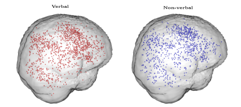
Figure 1: Graphical representation of the meta-analysis dataset. Data consist of 2,107 foci from 157 studies on working memory. Of these, 1,207 are obtained from studies using verbal stimuli (shown in red) whereas the remaining 900 are obtained from studies using non-verbal stimuli (shown in blue). The code used to generate this figure is courtesy of Jian Kang.

Our meta-analysis aims to address the following questions related to the function of working memory: I) what the regions of the brain that are consistently engaged by working memory across studies? II) do these regions differ depending on the type of stimulus presented to the participants? III) is the organisation of working memory affected by age? IV) does sample size affect the total number of activations reported? In order to ensure that the answers to these questions are not driven by influential publications conducting multiple studies, our investigations should account for such dependencies.

3 A model for CBMA meta-regression

To address the questions raised in Section 2, we propose a model for CBMA meta-regression. First, we set notation. Suppose that there are a total $I$ studies in the meta analysis and that each study $i$ comes with a point pattern $\mathbf{x}_{i}$, a set of foci $x_{ij}\in\mathcal{B}\subset\mathbb{R}^{3}$, where $\mathcal{B}$ is the support of the analysis, usually set from a standard atlas of the brain, and $j=1,\dots,n_{i}$, where $n_{i}$ is the number of foci in a study. Additionally, suppose that for each point pattern there is a set of $K$ study specific characteristics, $\left\{z_{ik}\right\}_{k=1}^{K}$. Henceforth, we will occasionally refer to these characteristics as covariates.

We assume that each point pattern $\mathbf{x}_{i}$ is the realisation of a Cox point process $\mathbf{X}_{i}$ defined on $\mathcal{B}$, driven by a random intensity $\lambda_{i}(\cdot)$. We can then model the intensity function at each point $\xi\in\mathcal{B}$ as

$$\lambda_{i}(\xi) = \alpha_{i}\exp{\left\{\sum_{k=0}^{K^{\ast}}{\beta_{k}(\xi)z_{ik}}+\sum_{k=K^{\ast}+1}^{K}{\beta_{k}z_{ik}}\right\}},$$ (1)

where $\alpha_{i}$ is the random effect of study $i$, $\beta_{k}(\cdot)$ are the regression coefficients for the covariates that have a local effect ($k=0,\dots,K^{\ast}$), $z_{ik}$ are covariate values where $k=0$ is for the intercept ($z_{i0}=1$), and are $\beta_{k}$ the regression coefficients for the covariates that have a global (homogenous) effect ($k=K^{\ast}+1,\dots,K$).

Equation (1) defines a spatial log-linear model over the brain. Foci are more likely to occur in regions of the brain with high intensity values whereas we expect almost no foci in regions as the intensity approaches zero. The exact rates are given by the properties of a Cox process. In particular, given $\lambda_{i}(\cdot)$, the expected number of foci in any bounded $B\subseteq\mathcal{B}$ is a Poisson random variable with mean $\int_{B}\lambda_{i}(\xi)d\xi$ (Møller and Waagepetersen, 2004).

The inclusion of the random effect terms is an important feature of our model. Firstly, by assuming that $\alpha_{i}=\alpha_{j}$ for studies $i$ and $j$ retrieved from the same publication, we relax the assumption of independence between their reported activations. This assumption is taken by all existing CBMA approaches but is unlikely to hold for studies from the same publication. For example, a multi-study publication will typically engage the same participants in all of its experiments. By using a common random effect for studies from the same publication, our model prevents publications with several studies to drive the estimates of the regression coefficients. Secondly, the random effects can allow for additional variability in the total number of foci that cannot be captured by the Poisson log-linear model. In a recent study, Samartsidis et al. (2017) found that CBMA data do show such overdispersion and thus inclusion of the random effect terms can potentially improve the fit to the data.

Separation of the covariates into those with a localised and those with a global effect should be done with caution. If one is interested in investigating whether the effect of a covariate varies from one region of the brain to another, such as age in our application, a spatially varying regression coefficient is needed. However, the total number of parameters associated with a spatially varying effect is large and therefore assigning a spatially varying coefficient to a covariate with a global effect may substantially increase the uncertainty associated to the other model parameters. In order to determine if a spatially varying coefficient for a covariate is required, one can fit two models, one that assumes that the covariate has a global effect and one that assumes a local effect. If the more complex model improves the fit to the data substantially, then it should be preferred for inference instead of the simple model. Sometimes, it plausible to assume a global effect solely based on prior expectation. For instance, a covariate for multiple testing correction can be assumed to have a global effect; for studies not applying any corrections, we expect false positives to appear uniformly across the brain.

A Bayesian model is defined with prior distributions on model parameters, which here include the functional parameters $\beta_{k}(\cdot)$ ($k=0,\ldots,K^{\ast}$), and scalar parameters $\beta_{k}$, ($k=K^{\ast}+1,\ldots,K$). A natural way to proceed is to assume that $\beta_{k}(\cdot)$ are realisations of Gaussian processes and that the $\beta_{k}$ have normal distributions. That way, when $\alpha_{i}=1$, the right hand side of Equation (1) is also a Gaussian process, and each point process is a log-Gaussian Cox process (LGCP) (Møller et al., 1998). The log-Gaussian Cox process is a flexible model for spatial point data that can account for aggregation (Møller et al., 1998; Møller and Waagepetersen, 2007) or even repulsion between points (Illian et al., 2012a) and has therefore found applications in several fields such as disease mapping (Benes et al., 2002; Liang et al., 2009) and ecology (Møller and Waagepetersen, 2003; Illian et al., 2012b).

By the definition of a Cox process, $\mathbf{X}_{i}$ is a Poisson point process on $\mathcal{B}$ conditional on $\lambda_{i}(\cdot)$ (Møller and Waagepetersen, 2004). The density (Radon-Nikodym derivative) of this point process with respect to the unit rate Poisson process is

$$\pi\left(\mathbf{x}_{i}|\lambda_{i}\right)=\exp{\left\{|\mathcal{B}|-\int_{\mathcal{B}}{\lambda_{i}(\xi)d\xi}\right\}}\prod_{x_{ij}\in\mathbf{x}_{i}}\lambda_{i}(x_{ij}),$$ (2)

for $i=1,\dots,I$, with $|\mathcal{B}|$ denoting the volume of the brain. We can view $\pi\left(\mathbf{x}_{i}\mid\lambda_{i}\right)$ as the density of the sampling distribution of the data. If we further assume independent studies, then we posterior distribution of the model parameters conditional on the foci is given, up to a normalising constant by

$$\pi\left(\left\{\alpha_{i}\right\}_{i=1}^{I},\left\{\beta_{k}(\cdot)\right\}_{k=0}^{K^{\ast}},\left\{\beta_{k}\right\}_{k=K^{\ast}+1}^{K}\mid\left\{\mathbf{x}_{i}\right\}_{i=1}^{I}\right)\propto\prod_{i=1}^{I}{\pi(\mathbf{x}_{i}|\lambda_{i})}\\ \times\prod_{i=1}^{I}{\pi(\alpha_{i})}\prod_{k=1}^{K^{\ast}}{\pi(\beta_{k}(\cdot))}\prod_{k=K^{\ast}+1}^{K}{\pi(\beta_{k})},$$ (3)

where $\pi(\alpha_{i})$, $\pi(\beta_{k}(\cdot))$ and $\pi(\beta_{k})$ are the priors on the random effects, functional and scalar parameters, respectively, which we discuss the priors below in Section 3.2.

3.1 Choice of correlation function

We will assume an isotropic, Gaussian correlation structure, that is for points $\xi,\xi^{\prime}\in\mathcal{B}$ we have

$$\mathbb{C}\mathrm{or}\left(\beta_{k}(\xi),\beta_{k}(\xi^{\prime})\right)=\exp{\left\{-\rho_{k}||\xi-\xi^{\prime}||^{\delta_{k}}\right\}},$$ (4)

where $\rho_{k}>0$ are the correlation decay parameters and $\delta_{k}=2$ for all $k=1,\dots,K^{\ast}$. Note that for numerical stability with the discrete Fourier transform (see Section 4) we set $\delta=1.9$ in our implementations. The same correlation structure was used by Møller et al. (1998) and Møller and Waagepetersen (2003) in the context of LGCPs.

A Gaussian correlation function is used instead of alternative correlation structures (see e.g. Rasmussen and Williams (2005)) because it allows us to calculate the gradient of the posterior with respect to the correlation parameters $\rho_{k}$, which we use to design an efficient algorithm for posterior simulations (see Section 4 for details). Further, in exploratory work using other correlation structures, our neuroscientist colleagues preferred the appearance of results from Gaussian correlation, perhaps because of the pervasive use of Gaussian kernel smoothing in fMRI. Finally, it is well known that estimating the correlation parameters for more flexible correlation structures can be extremely challenging in practice, see e.g. discussions by Zhang (2004) and Diggle et al. (2013) for the Matérn correlation function.

3.2 Posterior approximation

Calculation of the posterior in Equation (3) requires the evaluation of the infinite dimensional Gaussian processes $\beta_{k}\left(\cdot\right)$, $k=0,\dots,K^{\ast}$, which we approximate with a finite dimensional distribution. Following Møller et al. (1998) and Benes et al. (2002), we consider the discretisation of the 3D volume with a regular rectangular grid $W\supset\mathcal{B}$. We use $V$ cubic cells (i.e. voxels) in $W$ with volume $A=a^{3}$, where $a$ is the length of the side. In neuroimaging, analysis with $2\mathrm{mm}^{3}$ cubic voxels is typical, leading to a box-shaper grid of about 1 million voxels, of which about 200,000 are in the brain or cerebellum. Note that for simplicity, we consider both grey matter and white matter voxels in our implementations. Voxels are indexed $v=1,\ldots,V$, and the coordinate of $v$ is the location of the center $\boldsymbol{\nu}_{v}\in\mathbb{R}^{3}$.

For any $k=0,\dots,K^{\ast}$, the Gaussian process $\beta_{k}(\cdot)$ can be now approximated with a step function which is constant within each voxel $v$ and equal to the value of $\beta_{k}(\cdot)$ at the location of the center, i.e. $\beta_{k}(\boldsymbol{\nu}_{v})$. Waagepetersen (2004) shows that the accuracy of this approximation improves as $a$ goes to zero. By definition, $\boldsymbol{\beta}_{k}=\left[\beta_{k}(\boldsymbol{\nu}_{1}),\dots,\beta_{k}(\boldsymbol{\nu}_{V})\right]$ are multivariate Gaussian vectors. We parametrise $\boldsymbol{\beta}_{k}$ as

$$\boldsymbol{\beta}_{k}=\mu_{k}\mathbf{1}_{V}+\sigma_{k}\mathbf{R}_{k}^{1/2}\boldsymbol{\gamma}_{k},$$ (5)

where $\mu_{k}$ are the overall (scalar) means, $\mathbf{1}_{V}$ is a $V$-vector of ones, $\sigma_{k}$ are the marginal standard deviations, $\mathbf{R}_{k}$ are the $V\times V$ correlation matrices with elements $\left(\mathbf{R}_{k}\right)_{ij}=\exp{\left\{-\rho_{k}||\boldsymbol{\nu}_{i},\boldsymbol{\nu}_{j}||^{2}\right\}}$, and $\boldsymbol{\gamma}_{k}$ are the a priori $\mathcal{N}_{V}(\mathbf{0},\mathbf{I}_{V})$ vectors, $k=0,\dots,K^{\ast}$. The same parametrisation is used by Møller et al. (1998), Christensen and Waagepetersen (2002) and is advocated by Christensen et al. (2006) because it allows for computationally efficient posterior simulations.

Priors for the $V$-vectors $\boldsymbol{\gamma}_{k}$ are induced by the parametrisation of Equation (5). The priors for the remaining model parameters are set as follows. We assign weakly informative $\mathcal{N}\left(0,10^{8}\right)$ to the scalar parameters $\mu_{k}$, $\sigma_{k}$ and $\beta_{k}$. Further, we assume that $\rho_{k}\sim\mathrm{Uni}\left[3.5\times 10^{-3},0.1\right]$, which we found corresponded to smoothness ranges found in single-study fMRI statistic maps. Finally, in order to ensure identifiability, we a priori let $\alpha_{i}\sim\mathcal{G}(\kappa,\kappa)$. In our analyses, we set $\kappa=10$ since we expect 90% of the multiplicative random effects to be within the interval $[0.5,1.5]$.

Once the latent Gaussian processes are approximated, one can also approximate $\lambda_{i}$ with a step function as before. The intensities at the center of each voxel are given by

$$\boldsymbol{\lambda}_{i}=\alpha_{i}\exp{\left\{\sum_{k=0}^{K^{\ast}}{\left(\mu_{k}\mathbf{1}_{V}+\sigma_{k}\mathbf{R}^{1/2}_{k}\boldsymbol{\gamma}_{k}\right)z_{ik}}+\sum_{k=K^{\ast}+1}^{K}{\beta_{k}z_{ik}}\mathbf{1}_{V}\right\}},$$ (6)

where $\boldsymbol{\lambda}_{i}$ is the $V$-vector, the discretised intensity. We will write $\lambda_{iv}=(\boldsymbol{\lambda}_{i})_{v}$ for the $v$-element of study $i$’s intensity. The approximated posterior is

$$\pi\left(\boldsymbol{\theta}\mid\left\{\mathbf{x}_{i}\right\}_{i=1}^{I}\right)\propto\prod_{i=1}^{I}{\left[\exp{\left\{-\sum_{v}{A_{v}\lambda_{iv}}\right\}}\prod_{j=1}^{n_{i}}{\lambda_{iv(x_{ij})}}\right]}\pi(\boldsymbol{\theta}),$$ (7)

where $\boldsymbol{\theta}=\left\{\left\{\alpha_{i}\right\}_{i=1}^{I},\left\{\mu_{k}\right\}_{k=1}^{K^{\ast}},\left\{\sigma_{k}\right\}_{k=1}^{K^{\ast}},\left\{\rho_{k}\right\}_{k=1}^{K^{\ast}},\left\{\boldsymbol{\gamma}_{k}\right\}_{k=1}^{K^{\ast}},\left\{\beta_{k}\right\}_{k=K^{\ast}+1}^{K}\right\}$, $A_{v}$ takes on the value $A$ when $\boldsymbol{\nu}_{v}\in\mathcal{B}$ and 0 otherwise, $v(x_{ij})$ is the index of the voxel containing $x_{ij}$, and $\pi(\boldsymbol{\theta})$ is the joint prior distribution of the parameters. The posterior distribution in Equation (7) is still analytically intractable due to the presence of an unknown normalising constant and thus we need to resort to Monte Carlo simulation or approximation techniques to obtain samples from it. The method that we use is described in Section 4.

4 Sampling algorithm details

Bayesian methodology for inference on LGCPs can be broadly divided into two main categories: simulation based approximations of the posterior such as Markov chain Monte Carlo (Møller et al., 1998, MCMC) and elliptical slice sampling (Murray et al., 2010), and deterministic approximations to the posterior such as integrated nested Laplace approximations (Illian et al., 2012a; Simpson et al., 2016, INLA) and variational Bayes (Jaakkola and Jordan, 2000). In a recent study, Taylor and Diggle (2014) compare the Metropolis-adjusted Langevin (MALA) algorithm with INLA and find that both methods give similar results. In our application, we choose to use simulation based methods because application on our 3D problem is more straightforward.

We propose a hybrid MCMC algorithm to sample from the posterior (7), where parameters are updated in two blocks. The first block includes the random effect terms $\boldsymbol{\alpha}=\left\{\alpha_{i}\right\}_{i=1}^{I}$, whereas the second block includes the remaining model parameters $\boldsymbol{\theta}^{\ast}=\boldsymbol{\theta}\setminus\boldsymbol{\alpha}$. The gamma prior is conjugate for the elements of $\boldsymbol{\alpha}$; hence, they are simulated from their full conditional distributions given the remaining model parameters, see Appendix A.5 for details. Even though it is possible, we choose not to update $\boldsymbol{\alpha}$ jointly with $\boldsymbol{\theta}^{\ast}$ because that would increase computation time of our algorithm.

Sampling from the full conditional of $\boldsymbol{\theta}^{\ast}$ given $\boldsymbol{\alpha}$ is challenging due to its dimensionality. Girolami and Calderhead (2011) showed that of all possible strategies, their Riemann manifold Hamiltonian Monte Carlo (RMHMC) sampler is the computationally most efficient for LGCPs in a 2D setting. Unfortunately, application in this problem (3D setting) is prohibitive as it would require the inversion of a huge $V\times V$ tensor matrix. Alternatives to RMHMC include the MALA and the standard Hamiltonian Monte Carlo (Duane et al., 1987; Neal, 2011, HMC) algorithms. We choose to use HMC because Girolami and Calderhead (2011) found that it is more efficient compared MALA in a 2D setting. This finding was confirmed in our preliminary 2D simulation studies with synthetic CBMA data, where HMC outperformed MALA in terms of computational efficiency (mixing/running-time tradeoff).

HMC initially appeared in the physics literature by Duane et al. (1987) under the name hybrid Monte Carlo, and later emerged into statistics literature by Neal (2011). HMC emulates the evolution of a particle system which is characterised by its position ($\mathbf{q}$) and momentum ($\mathbf{p}$) over time. In our case, $\mathbf{q}$ will be the parameter vector of interest $\boldsymbol{\theta}^{\ast}$, and $\mathbf{p}$ will be introduced artificially from a $\mathcal{N}_{d}(0,\mathbf{M})$ distribution, with $d$ being the dimensionality of the problem and $\mathbf{M}$ the mass matrix. The dynamics of the system are described by a set of differential equations, known as Hamilton’s equations.

HMC alternates between moves for the position vector $\boldsymbol{\theta}^{\ast}$ and the momentum vector $\mathbf{p}$ based on Hamilton’s equations. If the solutions of the equations can be found analytically then moves will be deterministic; if not, numerical integration is required and an acceptance/rejection step must be performed to account for integration error. Integration is done in fictitious time $\epsilon L$, where $\epsilon$ is the stepsize and $L$ is the number of steps. Typically the leapfrog integrator is employed, which for $L=1$ and starting at time $t$ is performed as (Neal, 2011)

$$\mathbf{p}\left(t+\frac{\epsilon}{2}\right) = \mathbf{p}\left(t\right)+\frac{\epsilon}{2}\nabla_{\boldsymbol{\theta}^{\ast}}\log{\pi\left(\boldsymbol{\theta}^{\ast}(t)\mid\left\{\mathbf{x}_{i}\right\}_{i=1}^{I},\boldsymbol{\alpha}\right)}$$

$$\boldsymbol{\theta}^{\ast}\left(t+\epsilon\right) = \boldsymbol{\theta}^{\ast}\left(t\right)+\epsilon\mathbf{M}^{-1}\mathbf{p}\left(t+\frac{\epsilon}{2}\right)$$ (8)

$$\mathbf{p}\left(t+\epsilon\right) = \mathbf{p}\left(t+\frac{\epsilon}{2}\right)+\frac{\epsilon}{2}\nabla_{\boldsymbol{\theta}^{\ast}}\log{\pi\left(\boldsymbol{\theta}^{\ast}(t+\epsilon)\mid\left\{\mathbf{x}_{i}\right\}_{i=1}^{I},\boldsymbol{\alpha}\right)}.$$

Overall, if the method is applied correctly, it will produce samples from the desired full conditional distribution $\pi\left(\boldsymbol{\theta}^{\ast}\mid\left\{\mathbf{x}_{i}\right\}_{i=1}^{I},\boldsymbol{\alpha}\right)$. Gradient expressions for the elements of $\boldsymbol{\theta}^{\ast}$, including correlation parameters $\rho_{k}$, can be found in Appendix A. Since it is well known that grouping of variables can lead to samplers with faster convergence properties (Park and van Dyk, 2009), we choose to update all elements of $\boldsymbol{\theta}^{\ast}$ jointly using the HMC. The solutions to Hamilton’s equations are not available analytically so we need to use the Leapfrog integrator and include an accept/reject step at the end of it.

Our sampler requires the specification of a stepsize $\epsilon$ and a total number of leapfrog steps $L$ for the HMC step. Hoffman and Gelman (2014) show how tuning can be achieved automatically but when we applied this method to our problem running time was increased substantially. Therefore we use an alternative approach to tune these parameters. The stepsize is automatically adjusted during the burn-in phase of the HMC to give an overall acceptance rate close to the $65\%$ suggested by Neal (2011). In particular, if $\epsilon_{t}$ is the stepsize at iteration $t$ and $q_{t_{1}}$ is the acceptance rate over the past $t_{1}$ iterations, then every $t_{2}$ iterations we calculate the new stepsize $\epsilon_{t}^{\prime}$ as

$$\epsilon_{t}^{\prime}=\begin{cases}0.9\epsilon_{t}&q_{t_{1}}<0.60\\ \epsilon_{t}&0.60\leq q_{t_{1}}\leq 0.70\\ 1.1\epsilon_{t}&q_{t_{1}}>0.70\end{cases}.$$ (9)

Specifically we use $t_{1}=100$ and $t_{2}=10$. A similar approach is employed by Marshall and Roberts (2012) for MALA. The latter (number of leapfrog steps), is always fixed to $L=50$. We took this approach because we found that, for our LGCP application, the mixing properties of the algorithm scale linearly with $L$ but also with the total number of HMC iterations. Hence one can use a relatively large $L$ and few iterations or relatively smaller $L$ and more iterations, the total computation time staying relatively constant.

The last tuning parameter in the HMC algorithm is the variance-covariance matrix of the zero mean normal momentum parameters, $\mathbf{M}$. To our knowledge, there is only limited off the shelf methodology on how to adjust $\mathbf{M}$. As a starting place we set $\mathbf{M}=\mathbf{I}$. Neal (1996) suggests that if an estimate of the posterior variance $\hat{\boldsymbol{\Sigma}}_{\boldsymbol{\theta}^{\ast}}$ is available then a good practice is to set $\mathbf{M}=\hat{\boldsymbol{\Sigma}}_{\boldsymbol{\theta}^{\ast}}^{-1}$. In principle, $\hat{\boldsymbol{\Sigma}}_{\boldsymbol{\theta}^{\ast}}$ can be estimated during the burn-in phase of HMC but in practice this is not possible due to the dimensionality of the problem. In our simulations, we found that the mean posterior variance of the elements of the $\boldsymbol{\gamma}_{k}$ was higher compared to the scalar parameters, followed by $\beta_{k}$ or $\sigma_{k}$ and then $\rho_{k}$. Especially for the $\rho_{k}$ the scale is typically much smaller compared to the other parameters in our applications and so we use $100\times\rho_{k}$ instead of $\rho_{k}$. After the reparametrisation we found that setting the mass for parameters of $\boldsymbol{\gamma}_{k}$, $\beta_{k}$, $\sigma_{k}$ and $\rho_{k}$ equal to 1, 9, 16 and 25 respectively worked well in most of our implementations on simulated and real data. However, users might need to adjust these parameters if mixing of the chains is slow. For example, estimates of the posterior variance of the scalar parameters can be obtained based on preliminary runs of the algorithm for a few iterations. In Appendix B, we perform a series of simulations studies which demonstrate that the proposed HMC algorithm can efficiently sample from the posterior distribution of the high-dimensional parameter vector $\boldsymbol{\theta}^{\ast}$.

The most computationally demanding part of the algorithm is the the calculation of the large matrix-vector products $\mathbf{R}^{1/2}_{k}\boldsymbol{\gamma}_{k}$ appearing in the intensity functions of Equation (6). Luckily, an elegant solution to this problem is given by Møller et al. (1998) based on circulant embedding that was first proposed by Dietrich and Newsam (1993) and Wood and Chan (1994). The key to the approach is the linear algebra result that a circulant matrix has the discrete Fourier basis as its eigenvectors. $\mathbf{R_{k}}$ is not circulant but is block Toeplitz and can be embedded in a $(2V)\times(2V)$ matrix that is circulant. Thus the matrix square root, inversion and multiplication can be accelerated by using (the highly efficient) discrete Fourier transform (DFT) of the embedded matrix and manipulating Fourier coefficients, followed by inverse DFT and extracting the appropriate sub-matrix/sub-vector. See Rue and Held (2005, Section 2.6.2) for more details.

We close this section by stressing that despite the massive dimensionality of the parameter vector, the problem has a very high degree of parallelisation. Intensities can be evaluated in blocks of thousands of voxels simultaneously making the algorithm suitable for implementation in a graphics processing unit (GPU). The most computationally intensive part of our model, namely operations with DFTs, is also amenable to parallelisation and there exist libraries such as NVIDIA’s cuFFT library that are designed for this specific task. Overall, we believe that implementation of the log-Gaussian Cox process model described above will soon become a routine task for any moderately powerful GPU device.

5 Analysis of the WM dataset

5.1 Model, algorithm details and convergence diagnostics

For $i=1,\dots,157$ we fit the model

$$\boldsymbol{\lambda}_{i}=\alpha_{i}\exp\Big{\{}\boldsymbol{\beta}_{0}d_{i0}+\boldsymbol{\beta}_{1}d_{i1}+\boldsymbol{\beta}_{2}\mathrm{age_{i}}+\beta_{3}\frac{1}{\sqrt{n_{i}}}\mathbf{1}_{V}\Big{\}},$$ (10)

where $d_{i0}$ and $d_{i1}$ are indicator variables of verbal and non-verbal stimuli, respectively, and $n_{i}$ is the total number of participants in study $i$. Continuous parameters were standardised before implementation.

We run the MCMC algorithm described in Section 4 for 22,000 iterations, discarding the first 7,000 as a burn-in. The algorithm run for approximately 30 hours on an NVIDIA Tesla K20c GPU card. We then apply a thinning factor of 15 to the chains and therefore end up with 1,000 draws from the posterior distribution of the model parameters. The total number of leapfrog steps is set to $L=50$ and the stepsize is initialised at $\epsilon=0.00001$. We use a diagonal mass matrix with units specified in Section 4. A preliminary run of the algorithm revealed that the posterior variance of the scalar parameters $\rho_{2}$ and $\sigma_{2}$ of $\boldsymbol{\beta}_{2}$ was higher compared to the corresponding parameters of $\boldsymbol{\beta}_{0}$ and $\boldsymbol{\beta}_{1}$. Therefore, in order to improve mixing of the algorithm, we set the mass parameters to 1 and 4 for $\rho_{2}$ and $\sigma_{2}$, respectively.

Convergence of the MCMC chain is assessed visually by inspection of posterior traceplots for the model parameters. We run a total of 2 MCMC chains in order to examine if they all converge to the same values. Posterior traceplots are shown in Appendix C. Due to the large number of parameters we mainly focus on the scalar parameters of the model and some summary statistics, see Appendix C for more details. Results indicate that our chains have converged to their stationary distribution. This is verified by the fact that posterior values from the 2 different runs overlap one with another for all the quantities that we examine.

5.2 Results

Figure 2 shows the mean posterior of $\boldsymbol{\lambda}$, the average intensity of a working memory study, where $\boldsymbol{\lambda}=(\boldsymbol{\lambda}_{\mathrm{v}}+\boldsymbol{\lambda}_{\mathrm{nv}})/2$, $\boldsymbol{\lambda}_{\mathrm{v}}$ is the intensity for verbal WM studies and $\boldsymbol{\lambda}_{\mathrm{nv}}$ is for non-verbal WM studies (mean age and number of participants are set equal equal to the average values in our dataset). We can see that working memory engages several regions of the brain. The regions mostly activated are the frontal orbital cortex (axial slice $z=-10$, left), the insular cortex ($z=-10$, right and $z=-2$, left and right), the precentral gyrus ($z=+30$, left), Broca’s areas ($z=+22$ & $z=+30$, bilateral), the angular gyrus ($z=+46$, left), the superior parietal lobule ($z=+46$, right) and the paracingulate gyrus ($z=+46$, middle).

Our results are qualitatively similar to results obtained by Rottschy et al. (2012) who used the ALE method. However, our model-based approach allows us to derive several quantities of interest along with credible intervals, that cannot be obtained by any of the kernel-based methods. For example, one may calculate the probability of observing at least one focus in a set of voxels, e.g. an ROI or the entire brain. Table LABEL:tab:roi summarises the posterior distribution of $\mathbb{P}(N_{\mathbf{X}}(B)\geq 1)$, the probability of observing at least one focus in $B$, for several ROIs $B$. A full brain analysis can be found in Appendix D. The division of the brain in ROIs is done according to the Harvard-Oxford atlas (Desikan et al., 2006).

Table 2: Posterior % probabilities of observing at least once focus for several ROIs. All quantities have been calculated based on 1,000 MCMC samples.

ROI	Mean	95% CI	Verbal	Non-verbal
Frontal orbital cortex	36.94	[27.27,43.06]	37.26	36.48
Insular cortex	33.39	[26.68,39.36]	32.79	33.86
Precentral gyrus	68.47	[59.96,73.72]	64.10	72.09
Inferior frontal gyrus, PO	39.88	[31.06,45.96]	43.66	35.69
Angular gyrus	21.69	[14.39,26.34]	24.30	18.91
Superior parietal lobule	36.16	[26.16,42.31]	38.81	33.24
Paracingulate gyrus	46.22	[35.94,52.89]	42.91	49.14

We use posterior intensities $\boldsymbol{\lambda}_{\mathrm{v}}$ and $\boldsymbol{\lambda}_{\mathrm{nv}}$ to compare activation between the two types of studies in our sample, namely studies using verbal and studies non-verbal stimuli. We start with an ROI analysis. In particular, for each type and ROI we calculate the probability of at least one focus observed as explained above. These are shown in Table LABEL:tab:roi for a few ROIs, whereas a full brain analysis of the two types can be found in Appendix D. We see that even though the two types show similar patterns of activation, there several ROIs where the probabilities of at least one focus have credible intervals with little overlap. The main differences are found in the superior frontal gyrus, the middle frontal gyrus, the lateral occipital cortex, superior division and the inferior frontal gyrus, pars opercularis. A voxel-by-voxel comparison is also feasible. To answer this, we use the mean standardised posterior difference $\frac{\beta_{0v}-\beta_{1v}}{\mathrm{sd}\left(\beta_{0v}-\beta_{1v}\right)}$. This is shown in Figure 3. Large positive values indicate regions that are activated by verbal stimuli more than non-verbal stimuli. Such regions appear the occipital fusiform gyrus ($z=-18$, right). Based on the mean standardised posterior difference, regions mostly activated in studies using non-verbal are located in the middle frontal gyrus ($z=+46$).

Our results provide evidence that age has an important effect on the function of working memory. The point estimate for the overall age effect $\mu_{2}$ is -0.22 (95% CI [-0.337,-0.120]) thus suggesting that we expect a decrease of 20% in the total number of reported activations per study, each time the average age of the participants increases by 10.99 years. Localised age effects can be identified through the posterior distribution of $\exp{\left\{\boldsymbol{\beta}_{2}\right\}}$, the mean of which is shown in Figure 4. The map represents the multiplicative effect that an increase of the average participant age by 10.99 years has on the intensity of both verbal and non-verbal studies. Large negative age effects can be found near the left putamen ($z=-2$ and $z=-10$, middle), the insular cortex ($z=-2$, left) and near the superior parietal lobule ($z=+38$ and $z=+46$, right). A positive age effect is found near the precentral gyrus ($z=+30$, left). However, due to the limited number of studies, the posterior variance of these estimates is large in some regions of the brain, see Figure 14 of Appendix C.

The 95% CI for the sample size covariate is [-0.088,0.064] thus indicating that there is no significant effect on the total number of reported activations. The result is counter-intuitive as one would expect that studies with few participants would be underpowered and thus detect fewer activations. Thus, further investigation is required.

Figure 5 shows the mean posterior of the 89 unique random effect terms $\alpha_{i}$, one for each publication considered. We see that despite most of the mass being near 1, there are publications whose mean posterior random effect is different than 1, thus suggesting that observed variability of the foci counts is larger compared to what can be explained by the Poisson log-linear model. The importance of allowing for this additional variability can be seen by comparing the proposed random effects model to the standard LGCP model, which we also fit to the data. We use posterior predictive checks (Gelman et al., 1996) to assess how well the two models fit the data. For each study and MCMC draw, we simulate from the posterior predictive distribution of $N_{\mathbf{X}_{i}}(\mathcal{B})$, the total number of foci, given the covariates. Based on these draws, we calculate the 95% predictive intervals of $N_{\mathbf{X}_{i}}(\mathcal{B})$ and check if they contain the observed values. For our model, the coverage of the intervals is $90\%$ compared to $66\%$ obtained using the standard LGCP model, which implies that our model provides a better fit to the data compared to the standard LGCP. A comparison of the predictive intervals that takes into account the length of these intervals can be based on the mean interval score (Gneiting and Raftery, 2007). This is 22.45 and 76.93 for the random effects and standard LGCP models, respectively, thus suggesting that the inclusion of $\alpha_{i}$ leads to improved prediction of the study counts.

Some of the estimated effects are affected by inclusion of the random effect terms. For instance, the expected number of foci for verbal studies is estimated as 12.80 (95% CI [11.57,14.14]) by the random effects LGCP as opposed to 11.67 (95% CI [10.97,12.36]) by the fixed effects LGCP model. One possible explanation for this is that our model is assigning a low random effect to publications systematically reporting only a few foci. Such a behaviour is desired since, e.g.  this underreporting could be solely due to author preference. Further, the random effects model provides credible intervals that fully account for the uncertainty in the regression coefficients. For example, the 95% CI for the overall age effect $\mu_{2}$ provided by the fixed effects LGCP is [-0.309,-0.151], shorter than the CI provided by our model.

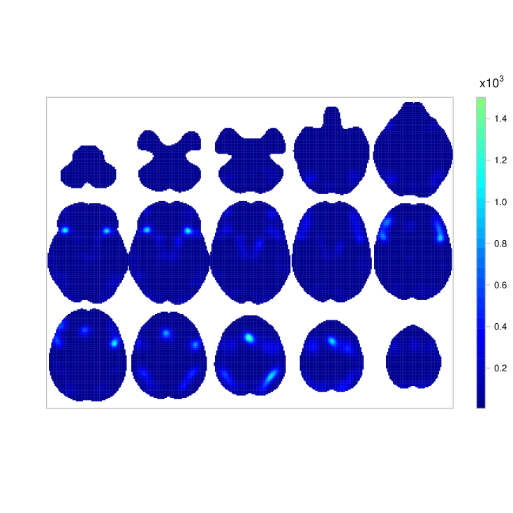
Figure 2: Voxelwise mean posterior of $\boldsymbol{\lambda}$, the average intensity of a working memory study. Top row shows (from left to right) axial slices $z=-50,-42,-34,-26$ and $-18$, respectively. Middle row shows axial slices $z=-10,-2,+6,+14$ and $+22$, respectively. Bottom row shows axial slices $z=+30,+38,+46,+54$ and $+62$, respectively.

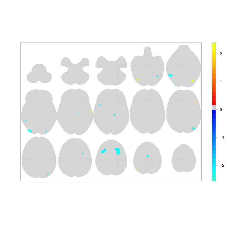
Figure 3: Voxelwise mean standardised posterior difference between $\boldsymbol{\beta}_{1}$ and $\boldsymbol{\beta}_{2}$, the intensities of studies using verbal and non-verbal stimuli, respectively. Top row shows (from left to right) axial slices $z=-50,-42,-34,-26$ and $-18$, respectively. Middle row shows axial slices $z=-10,-2,+6,+14$ and $+22$, respectively. Bottom row shows axial slices $z=+30,+38,+46,+54$ and $+62$, respectively. Voxels for which the mean posterior $\boldsymbol{\lambda}$ is low (below the 75% quantile over the brain) or the absolute mean standardised posterior difference is less than two have been set to zero.

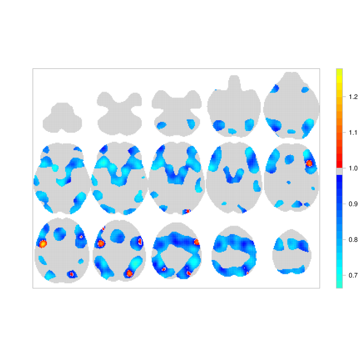
Figure 4: Mean posterior of $\exp{\left\{\boldsymbol{\beta}_{2}\right\}}$, the multiplicative age effect on the intensity of both verbal and non-verbal studies. Top row shows (from left to right) axial slices $z=-50,-42,-34,-26$ and $-18$, respectively. Middle row shows axial slices $z=-10,-2,+6,+14$ and $+22$, respectively. Bottom row shows axial slices $z=+30,+38,+46,+54$ and $+62$, respectively. Voxels for which the mean posterior $\boldsymbol{\lambda}$ is low (below the 75% quantile over the brain) have been set to one.

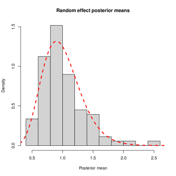
Figure 5: Histogram of the mean posterior random effect terms, $\alpha_{i}$. We only plot the 89 unique random effects, one for each publication considered in the meta-analysis. Means are based on a sample of 1,000 MCMC draws from the posterior. The dashed red line represents the density of the Gamma prior.

6 Discussion

In this work, we have presented a new CBMA model, extension of the log-Gaussian Cox process model. To our knowledge, this is the first application of the random effects LGCP with covariates in a 3D problem with multiple realisations. The model has an appealing interpretation being a spatial GLM and several interesting inferences can be obtained based on the properties of the spatial Poisson process that cannot be obtained with the commonly used kernel-based approaches. An advantage of our model compared to most of the existing methods is the inclusion of covariates in the analysis thus allowing for meta-regression. Finally, a novel feature introduced in our work is the inclusion of random-effect terms which can account for additional heterogeneity in the total number of activations, compared to the standard Poisson model.

Application of our model on a meta-analysis of working memory studies have given valuable insights regarding the data. While our maps for the overall pattern of WM activations (Fig. 2) and the differential effect of verbal vs. non-verbal WM tasks (Fig. 3) reflect previous findings found by Rottschy et al. (2012), our fully Bayesian approach allowed us to make direct inference on probability of any foci and expected number of foci. Our model found no regions with evidence of different rates of foci between verbal and non-verbal WM tasks (Appendix C, Table LABEL:tab:fullbrain2). Importantly, our model allows a meta-regression, and we examined the effect of age and found no strong effects but generally negative effects of age on the number of foci.

There are few limitations to our work. Firstly, even though we found that the proposed MCMC algorithm performed well in most of the applications considered, we believe that there is room for further for improvement. For example, one can consider adaptive schemes in order to automatically adjust the mass matrix $\mathbf{M}$ of the HMC which we found that is crucial for the mixing properties of the algorithm. Secondly, we are currently not considering the problem of learning the hyperparameter $\kappa$ that controls the posterior variability of the random effect terms, but rather make use of our prior expectations to tune it. However, since we found that results are sensitive to the specification of $\kappa$, it is plausible to consider estimating it along with remaining model parameters.

Our work can be extended in several ways. One possible direction for future research is to perform a head-to-head comparison of existing methodologies that can be used for posterior inference with the proposed LGCP model in the context of CBMA. However, given the computation time required to apply these methods to a 3D problem, such a comparison might be too long. Another potential future direction is to study the conditions, such as sample size or minimum number of foci, under which it is possible to estimate several global or spatially varying effects using the LGCP. Such work can be of importance for practical implementations since it will provide some guidance regarding the complexity of meta-regression models that can be fit to a given dataset.

Another open problem is how to use some additional information about the foci such as $p$-values or $T$-scores. These values can be attached as marks to the existing point patterns. Such an approach can enrich the inferences obtained from a CBMA by characterising the magnitude of activation in each region as opposed to the localisation of activations, which is the question that current methods address. Finally, it is worth considering a zero-truncated LGCP model. The reason is that several CBMAs use data from databases such as BrainMap (Laird et al., 2005), where only studies with at least one focus are registered. For such applications, a model that does not account for the zero-truncation can provide biased intensity estimates, especially when the expected number of foci per study is low. Currently, very few of the existing approaches propose adjustments for this potential problem.

Appendix A Gradient expressions for the LGCP

Let $\beta_{k}\equiv\mu_{k}$ ($k=0,\dots,K$). The log-posterior, up to a normalising constant is given by:

$$\ell\left(\boldsymbol{\alpha},\boldsymbol{\beta},\boldsymbol{\sigma},\boldsymbol{\rho},\left\{\boldsymbol{\gamma}_{k}\right\}_{k=1}^{K^{\ast}}\mid\cdot\right)\propto\sum_{i=1}^{I}{\left[-\sum_{j=1}^{V}{A_{v_{j}}\lambda_{i}(v_{j})}+\sum_{j=1}^{V}{\mathbf{1}_{v_{j}\in\mathbf{x}_{i}}\log{\lambda_{i}(v_{j})}}\right]}\\ +\log{\mathrm{priors}},$$ (11)

where $\boldsymbol{\alpha}=(\alpha_{1},\dots,\alpha_{I})^{\top}$, $\boldsymbol{\beta}=(\beta_{0},\dots,\beta_{K})^{\top}$, $\boldsymbol{\sigma}=(\sigma_{0},\dots,\sigma_{K^{\ast}})^{\top}$, $\boldsymbol{\rho}=(\rho_{0},\dots,\rho_{K^{\ast}})^{\top}$, $A_{v_{j}}=\mathbf{1}_{v_{j}\in\mathcal{B}}$ and the intensity function at each voxel $v_{j}$ is defined as:

$$\lambda_{i}(v_{j})=\alpha_{i}\exp{\left(\sum_{k=0}^{K}{\beta_{k}z_{ik}}\right)}\exp{\left(\sum_{k=0}^{K^{\ast}}{\sigma_{k}\left(\mathbf{R}^{1/2}_{k}\boldsymbol{\gamma}_{k}\right)_{j}z_{ik}}\right)}$$ (12)

We now calculate the derivatives with respect to the parameters of interest.

A.1 Partial derivatives with respect to $\beta_{l}$

We have that:

$$\frac{\partial\log{\lambda_{i}(v_{j})}}{\partial\beta_{l}} = \frac{\partial}{\partial\beta_{l}}\log{\alpha_{i}}+\frac{\partial}{\partial\beta_{l}}\sum_{k=0}^{K}{\beta_{k}z_{ik}}+\frac{\partial}{\partial\beta_{l}}\sum_{k=0}^{K^{\ast}}{\sigma_{k}\left(\mathbf{R}^{1/2}_{k}\boldsymbol{\gamma}_{k}\right)_{j}z_{ik}}$$ (13)

$$= z_{il}.$$

As a result:

$$\frac{\partial\ell\left(\beta_{l}\mid\cdot\right)}{\partial\beta_{l}} = -\sum_{i=1}^{I}{\sum_{j=1}^{V}{\left[A_{v_{j}}\frac{\partial}{\partial\beta_{l}}\lambda_{i}(v_{j})-\mathbf{1}_{v_{j}\in\mathbf{x}_{i}}\frac{\partial}{\partial\beta_{l}}\log{\lambda_{i}(v_{j})}\right]}}+\frac{\partial}{\partial\beta_{l}}\log{\pi(\beta_{l})}$$ (14)

$$= -\sum_{i=1}^{I}{\sum_{j=1}^{V}{\left[A_{v_{j}}\lambda_{i}(v_{j})z_{il}-\mathbf{1}_{v_{j}\in\mathbf{x}_{i}}z_{il}\right]}}-\frac{\partial}{\partial\beta_{l}}\frac{\beta_{l}^{2}}{2\tau^{2}}$$

$$= -\sum_{j=1}^{V}{\sum_{i=1}^{I}{A_{v_{j}}\lambda_{i}(v_{j})z_{il}}}+\sum_{i=1}^{I}n_{i}z_{il}-\frac{\beta_{l}}{\tau^{2}},$$

where $n_{i}$ is the total number of foci in study $i$.

A.2 Partial derivatives with respect to $\sigma_{l}$

We have that:

$$\frac{\partial\log{\lambda_{i}(v_{j})}}{\partial\sigma_{l}} = \frac{\partial}{\partial\sigma_{l}}\log{\alpha_{i}}+\frac{\partial}{\partial\sigma_{l}}\sum_{k=0}^{K}{\beta_{k}z_{ik}}+\frac{\partial}{\partial\sigma_{l}}\sum_{k=0}^{K^{\ast}}{\sigma_{k}\left(\mathbf{R}^{1/2}_{k}\boldsymbol{\gamma}_{k}\right)_{j}z_{ik}}$$ (15)

$$= \left(\mathbf{R}^{1/2}_{l}\boldsymbol{\gamma}_{l}\right)_{j}z_{il}.$$

Therefore:

$$\frac{\partial\ell\left(\sigma_{l}\mid\cdot\right)}{\partial\sigma_{l}} = -\sum_{i=1}^{I}{\sum_{j=1}^{V}{\left[A_{v_{j}}\frac{\partial}{\partial\sigma_{l}}\lambda_{i}(v_{j})-\mathbf{1}_{v_{j}\in\mathbf{x}_{i}}\frac{\partial}{\partial\sigma_{l}}\log{\lambda_{i}(v_{j})}\right]}}+\frac{\partial}{\partial\sigma_{l}}\log{\pi(\sigma_{l})}$$

$$= -\sum_{i=1}^{I}{\sum_{j=1}^{V}{\left[A_{{}_{v}j}\lambda_{i}(v_{j})\left(\mathbf{R}^{1/2}_{l}\boldsymbol{\gamma}_{l}\right)_{j}z_{il}-\mathbf{1}_{v_{j}\in\mathbf{x}_{i}}\left(\mathbf{R}^{1/2}_{l}\boldsymbol{\gamma}_{l}\right)_{j}z_{il}\right]}}-\frac{\partial}{\partial\sigma_{l}}\frac{\sigma_{l}^{2}}{2\tau^{2}}$$

$$= -\sum_{j=1}^{V}{\sum_{i=1}^{I}{\left[\left(\mathbf{R}^{1/2}_{l}\boldsymbol{\gamma}_{l}\right)_{j}\left(A_{v_{j}}\lambda_{i}(v_{j})z_{il}-\mathbf{1}_{v_{j}\in\mathbf{x}_{i}}z_{il}\right)\right]}}-\frac{\sigma_{l}}{\tau^{2}}$$

$$= -\sum_{j=1}^{V}{\left[\left(\mathbf{R}^{1/2}_{l}\boldsymbol{\gamma}_{l}\right)_{j}\sum_{i=1}^{I}{\left[A_{v_{j}}\lambda_{i}(v_{j})z_{il}-\mathbf{1}_{v_{j}\in\mathbf{x}_{i}}z_{il}\right]}\right]}-\frac{\sigma_{l}}{\tau^{2}}.$$

A.3 Partial derivatives with respect to $\rho_{l}$

Again:

$$\frac{\partial\log{\lambda_{i}(v_{j})}}{\partial\rho_{l}} = \frac{\partial}{\partial\rho_{l}}\log{\alpha_{i}}+\frac{\partial}{\partial\rho_{l}}\sum_{k=0}^{K^{\ast}}{\beta_{k}z_{ik}}+\frac{\partial}{\partial\rho_{l}}\sum_{k=0}^{K}{\sigma_{k}\left(\mathbf{R}^{1/2}_{k}\boldsymbol{\gamma}_{k}\right)_{j}z_{ik}}$$ (16)

$$= \sigma_{l}\frac{\partial}{\partial\rho_{l}}\left(\mathbf{R}^{1/2}_{l}\boldsymbol{\gamma}_{l}\right)_{j}z_{il}.$$

For ease of exposition we complete the derivation for the one-dimensional case; however, similar arguments can be used when $\mathcal{B}\subset\mathbb{R}^{3}$. Matrices $\mathbf{R}_{l}$ are circulant and so, the matrix-vector product $\mathbf{R}^{1/2}_{l}\boldsymbol{\gamma}_{l}$ can be found using the discrete Fourier transform as

$$\mathbf{R}^{1/2}_{l}\boldsymbol{\gamma}_{l}=\mathbf{F}\boldsymbol{\Phi}_{l}^{1/2}\mathbf{F}^{\mathrm{H}}\boldsymbol{\gamma}_{l},$$ (17)

where $\boldsymbol{\Phi}_{l}$ are the diagonal matrices containing the eigenvalues of $\mathbf{R}_{l}$ and $\mathbf{F}$ is the matrix of eigenvectors. In Equation (17), the only term depending on $\rho_{l}$ is $\boldsymbol{\Phi}_{l}$ and, hence:

$$\frac{\partial}{\partial\rho_{l}}\mathbf{R}^{1/2}_{l}\boldsymbol{\gamma}_{l}=\mathbf{F}\frac{\partial}{\partial\rho_{l}}\boldsymbol{\Phi}_{l}^{1/2}\mathbf{F}^{\mathrm{H}}\boldsymbol{\gamma}_{l}$$ (18)

We know that $\boldsymbol{\Phi}_{l}=\mathrm{diag}\left\{\phi_{l_{0}},\dots,\phi_{l_{V-1}}\right\}$, where for $k=0,\dots,V-1$ we have that:

$$\phi_{l_{k}}=\sum_{j=0}^{V-1}{\exp{\left(-\rho_{l}||v_{0},v_{j}||^{\delta_{l}}\right)}\exp{\left(-\frac{2\pi\iota kj}{V}\right)}},$$ (19)

where $\iota$ is the imaginary unit. Now it is straightforward to see that for $k=0,\dots,V-1$:

$$\frac{\partial}{\partial\rho_{l}}\phi_{l_{k}}^{1/2} = \frac{\partial}{\partial\rho_{l}}\sqrt{\sum_{j=0}^{V-1}{\exp{\left(-\rho_{l}||v_{0},v_{j}||^{\delta_{l}}\right)}\exp{\left(-\frac{2\pi\iota kj}{V}\right)}}}$$ (20)

$$= \frac{\frac{\partial}{\partial\rho_{l}}\sum_{j=0}^{V-1}{\exp{\left(-\rho_{l}||v_{0},v_{j}||^{\delta_{l}}\right)}\exp{\left(-\frac{2\pi\iota kj}{V}\right)}}}{2\sqrt{\sum_{j=0}^{V-1}{\exp{\left(-\rho_{l}||v_{0},v_{j}||^{\delta_{l}}\right)}\exp{\left(-\frac{2\pi\iota kj}{V}\right)}}}}$$

$$= \frac{-\sum_{j=1}^{V-1}{d\left(v_{0},v_{j}\right)^{\delta_{l}}\exp{\left(-\rho_{l}||v_{0},v_{j}||^{\delta_{l}}\right)}\exp{\left(-\frac{2\pi\iota kj}{V}\right)}}}{2\phi_{l_{k}}^{1/2}}$$

$$= -\frac{1}{2}\frac{\psi_{l_{k}}}{\phi_{l_{k}}^{1/2}},$$

where $\psi_{l_{k}}$ can be viewed as the $k$-th eigenvalue of the of a circulant matrix $\mathbf{S}_{l}$ with base $\mathbf{s}_{l}=\left[||v_{0},v_{0}||^{\delta_{l}}\exp{\left(-\rho_{l}||v_{0},v_{0}||^{\delta_{l}}\right)},\dots,||v_{0},v_{V-1}||^{\delta_{l}}\exp{\left(-\rho_{l}||v_{0},v_{V-1}||^{\delta_{l}}\right)}\right]$ and $\mathbf{S}_{l}=\mathbf{F}\boldsymbol{\Psi}_{l}\mathbf{F}^{\mathrm{H}}$, $\boldsymbol{\Psi}_{l}=\mathrm{diag}\left\{\psi_{l_{0}},\dots,\psi_{l_{V-1}}\right\}$. Overall we see that:

$$\frac{\partial}{\partial\rho_{l}}\mathbf{R}^{1/2}_{l}\boldsymbol{\gamma}_{l} = \mathbf{F}\frac{\partial}{\partial\rho_{l}}\boldsymbol{\Phi}_{l}^{1/2}\mathbf{F}^{\mathrm{H}}\boldsymbol{\gamma}_{l}$$ (21)

$$= -\frac{1}{2}\mathbf{F}\left[\boldsymbol{\Psi}_{l}\oslash\boldsymbol{\Phi}^{1/2}\right]\mathbf{F}^{\mathrm{H}}\boldsymbol{\gamma}_{l}$$

$$= -\frac{1}{2}\mathbf{Q}_{l}\boldsymbol{\gamma}_{l},$$

where $\oslash$ stands for element wise division. Combining Equations (16) and (21), we find that:

$$\frac{\partial\log{\lambda_{i}(v_{j})}}{\partial\rho_{l}}=-\frac{1}{2}\sigma_{l}\left(\mathbf{Q}_{l}\boldsymbol{\gamma}_{l}\right)_{j}z_{il}.$$ (22)

So:

$$\frac{\partial\ell\left(\rho_{l}\mid\cdot\right)}{\partial\rho_{l}} = -\sum_{i=1}^{I}{\sum_{j=1}^{V}{\left[A_{v_{j}}\frac{\partial}{\partial\rho_{l}}\lambda_{i}(v_{j})-\mathbf{1}_{v_{j}\in\mathbf{x}_{i}}\frac{\partial}{\partial\rho_{l}}\log{\lambda_{i}(v_{j})}\right]}}+\frac{\partial}{\partial\rho_{l}}\log{\pi(\rho_{l})}$$

$$= -\sum_{i=1}^{I}{\sum_{j=1}^{V}{\left[A_{{}_{v}j}\lambda_{i}(v_{j})\left(-\frac{1}{2}\right)\sigma_{l}\left(\mathbf{Q}_{l}\boldsymbol{\gamma}_{l}\right)_{j}z_{il}-\mathbf{1}_{v_{j}\in\mathbf{x}_{i}}\left(-\frac{1}{2}\right)\sigma_{l}\left(\mathbf{Q}_{l}\boldsymbol{\gamma}_{l}\right)_{j}z_{il}\right]}}$$

$$-\frac{\partial}{\partial\rho_{l}}\mathbf{1}_{\rho_{l}\in[\rho_{\mathrm{low}},\rho_{\mathrm{upp}}]}$$

$$= \frac{\sigma_{l}}{2}\sum_{j=1}^{V}{\sum_{i=1}^{I}{\left[\left(\mathbf{Q}_{l}\boldsymbol{\gamma}_{l}\right)_{j}\left(A_{v_{j}}\lambda_{i}(v_{j})z_{il}-\mathbf{1}_{v_{j}\in\mathbf{x}_{i}}z_{il}\right)\right]}}$$

$$= \frac{\sigma_{l}}{2}\sum_{j=1}^{V}{\left[\left(\mathbf{Q}_{l}\boldsymbol{\gamma}_{l}\right)_{j}\sum_{i=1}^{I}{\left[A_{v_{j}}\lambda_{i}(v_{j})z_{il}-\mathbf{1}_{v_{j}\in\mathbf{x}_{i}}z_{il}\right]}\right]}.$$

A.4 Partial derivatives with respect to $\boldsymbol{\gamma}_{l}$

Finally:

$$\frac{\partial\log{\lambda_{i}(v_{j})}}{\partial\boldsymbol{\gamma}_{l}} = \frac{\partial}{\partial\boldsymbol{\gamma}_{l}}\log{\alpha_{i}}+\frac{\partial}{\partial\boldsymbol{\gamma}_{l}}\sum_{k=0}^{K^{\ast}}{\beta_{k}z_{ik}}+\frac{\partial}{\partial\boldsymbol{\gamma}_{l}}\sum_{k=0}^{K}{\sigma_{k}\left(\mathbf{R}^{1/2}_{k}\boldsymbol{\gamma}_{k}\right)_{j}z_{ik}}$$ (23)

$$= \sigma_{l}\mathbf{r}_{l_{j}}z_{il},$$

where $\mathbf{r}_{l_{j}}$ is the $j$-th row of the matrix $\mathbf{R}_{l}^{1/2}$. Now we can see that:

$$\frac{\partial\ell\left(\boldsymbol{\gamma}_{l}\mid\cdot\right)}{\partial\boldsymbol{\gamma}_{l}} = -\sum_{i=1}^{I}{\sum_{j=1}^{V}{\left[A_{v_{j}}\frac{\partial}{\partial\boldsymbol{\gamma}_{l}}\lambda_{i}(v_{j})-\mathbf{1}_{v_{j}\in\mathbf{x}_{i}}\frac{\partial}{\partial\boldsymbol{\gamma}_{l}}\log{\lambda_{i}(v_{j})}\right]}}+\frac{\partial}{\partial\boldsymbol{\gamma}_{l}}\log{\pi(\boldsymbol{\gamma}_{l})}$$ (24)

$$= -\sum_{i=1}^{I}{\sum_{j=1}^{V}{\left[A_{v_{j}}\lambda_{i}(v_{j})\sigma_{l}\mathbf{r}_{l_{j}}z_{il}-\mathbf{1}_{v_{j}\in\mathbf{x}_{i}}\sigma_{l}\mathbf{r}_{l_{j}}z_{il}\right]}}-\frac{\partial}{\partial\boldsymbol{\gamma}_{l}}\frac{\boldsymbol{\gamma}_{l}^{\mathrm{T}}\boldsymbol{\gamma}_{l}}{2}$$

$$= -\sigma_{l}\sum_{j=1}^{V}{\left[\mathbf{r}_{l_{j}}\sum_{i=1}^{I}{\left[A_{v_{j}}\lambda_{i}(v_{j})z_{il}-\mathbf{1}_{v_{j}\in\mathbf{x}_{i}}z_{il}\right]}\right]}-\boldsymbol{\gamma}_{l}$$

$$= -\sigma_{l}\sum_{j=1}^{V}{\left[\mathbf{r}_{l_{j}}\mathbf{c}_{l_{j}}\right]}-\boldsymbol{\gamma}_{l}$$

$$= -\sigma_{l}\left(\mathbf{R}_{l}^{1/2}\right)^{\top}\mathbf{c}_{l}-\boldsymbol{\gamma}_{l}$$

$$= -\sigma_{l}\mathbf{R}_{l}^{1/2}\mathbf{c}_{l}-\boldsymbol{\gamma}_{l},$$

since $\mathbf{R}$ is a nested block circulant matrix, where $\mathbf{c}_{l}$ are $V$-vectors with elements $\mathbf{c}_{l_{j}}=\sum_{i=1}^{I}{\left[A_{v_{j}}\lambda_{i}(v_{j})z_{il}-\mathbf{1}_{v_{j}\in\mathbf{x_{i}}}z_{il}\right]}$.

A.5 Random effects updates

Let $J$ be the total number of publications from which the $I$ studies in the meta-analysis have been retrieved, and let $\mathcal{C}_{j}$ the set of studies retrieved from paper $j$ ($j=1,\dots,J$). For all $j=1,\dots,J$ we have that

$$\pi(\alpha_{j}|\cdot) \propto \pi(\alpha_{j})\prod_{i\in\mathcal{C}_{j}}\pi(\mathbf{x}_{i}|\lambda_{i})$$

$$\propto \alpha_{j}^{\kappa-1}\exp{\left\{-\alpha_{j}\kappa\right\}}\exp{\left\{-\alpha_{j}\sum_{i\in\mathcal{C}_{j}}\sum_{v=1}{\lambda_{iv}^{\ast}}\right\}}\alpha_{j}^{\sum_{i\in\mathcal{C}_{j}}n_{i}}$$

$$= \alpha_{j}^{\sum_{i\in\mathcal{C}_{j}}n_{i}+\kappa-1}\exp{\left\{-\alpha_{j}\left(\sum_{i\in\mathcal{C}_{j}}\sum_{v=1}{\lambda_{iv}^{\ast}}+\kappa\right)\right\}}.$$

Therefore, we draw $\alpha_{j}$ from a $\mathcal{G}\left(\sum_{i\in\mathcal{C}_{j}}n_{i}+\kappa,\sum_{i\in\mathcal{C}_{j}}\sum_{v=1}{\lambda_{iv}^{\ast}}+\kappa\right)$ distribution.

Appendix B Simulation studies

In order evaluate the performance of the proposed HMC algorithm to sample from the posterior distribution of the latent GPs, we consider two simulation setups. In the first we draw samples directly from the log-Gaussian Cox process model, whereas in the second we create synthetic studies based on a different model to assess its robustness to model misspecification. For consistency, all processesare defined on the same brain atlas used in the application of Section 5, consisting of 216,040 $2\mathrm{mm}^{3}$ cubic voxels. The average number of foci per simulated dataset is kept low (mean number of foci per study is 5) to resemble the sparsity of points observed in real CBMA data. Finally, the total number of studies is fixed to 200 in both analyses, similar to the sample sizes available in real applications (Kang et al., 2011, for example).

B.1 Setup 1

In this setting we simulate 200 studies, with two spatially varying covariates that account for the mean of two groups of studies, and two non-spatially varying covariates. For $i=1,\dots,200$ we set:

$$\lambda_{iv}=\exp{\left\{\sum_{k=1}^{2}{\left(\mu_{k}+\sigma_{k}\left(\mathbf{R}^{1/2}_{k}\boldsymbol{\gamma}_{k}\right)_{v}\right)z_{ik}}+\sum_{i=3}^{4}{\beta_{k}z_{ik}}\right\}},$$ (25)

where $z_{i1}\sim\mathrm{Bernoulli}(0.5)$, $z_{i2}=1-z_{i1}$, $z_{i3}\sim\mathrm{Uniform}[-1,1]$ and $z_{i4}\sim\mathrm{Bernoulli}(0.5)$. Note that this parametrisation of the covariates implies existence of two types of studies, say type 1 and 2, with different spatially varying means and the effect of one continuous and one categorical covariate. The expected total number of foci is 3.99 and 4.16 for studies of type 1 and 2 respectively. We draw $\boldsymbol{\gamma}_{1},\boldsymbol{\gamma}_{2}$ from their $\mathcal{N}_{V}(0,\mathbf{I})$ prior and fix the values of the scalar parameters shown in Table LABEL:tab:lgcpsim1. We run the HMC algorithm of Section 4 for 10,000 iterations, discarding the first 4,000 as a burn-in and save every 6 iterations for a total of 1,000 saved posterior samples. This took roughly 14 hours on an NVIDIA Tesla K20c GPU card.

Results are summarised in Table LABEL:tab:lgcpsim1 and Figure 8. In Table LABEL:tab:lgcpsim1 we see that the scalar parameters are estimated accurately despite the sparsity of points in the realisations. The 95% credible intervals contain the true values of all the parameters in the setup. Traceplots for the parameters $\sigma_{1}$, $\sigma_{2}$, $\rho_{1}$ and $\rho_{2}$ can be found in Figure 6, whereas trace plots for $\mu_{1}$, $\mu_{2}$, $\beta_{3}$ and $\beta_{4}$ can be found in Figure 7. The red lines indicate the true parameter values.

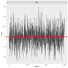
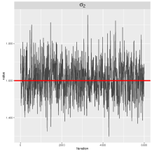
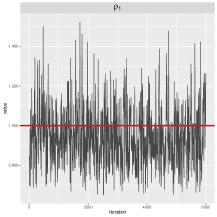
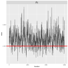
Figure 6: Posterior traceplots for the scalar parameters of the LGCP model used to fit the data of Section B.1. Top row: standard deviations. Bottom row: correlation decay parameters ($\times 100$). The true values are indicated by the solid red lines.

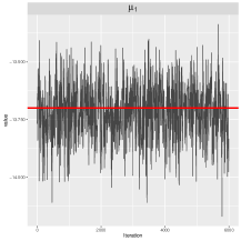
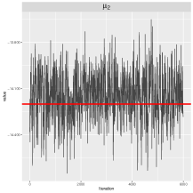
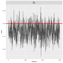
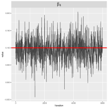
Figure 7: Posterior traceplots for the scalar parameters of the LGCP model used to fit the data of Section B.1. Top row: overall latent process means. Bottom row: regression coefficients for covariates $z_{3}$ and $z_{4}$. The true values are indicated by the solid red lines.

For $z_{i3}=z_{i4}=0$, the median expected number of points is 3.97 (95% CI [3.84,4.10])for type 1 and 4.61 (95% CI [4.46,4.78]) for type 2. These values are very similar to the values we observe in the simulated dataset, that is 3.98 for type 1 and 4.53 for type 2. This indicates that our model does a good job fitting the data. The shape of the latent Gaussian processes $\mu_{k}+\sigma_{k}\mathbf{R}^{1/2}_{k}\boldsymbol{\gamma}_{k}$ is generally captured for both types as can be seen in Figure 8. In particular, we can see that the maxima in the true and estimated images appear roughly in the same locations. The same cannot be said about the other values but this is expected given the dearth of information in regions of low intensity.

Table 3: Posterior summaries of the scalar parameters of the LGCP model, fit to the simulated data of Section B.1. Results are based on 1,000 posterior draws. The values for the correlation parameters $\rho_{1}$, $\rho_{2}$ are multiplied by 100. The values for $\beta_{1}$ and $\beta_{2}$ are multiplied by 10.

Parameter	True Value	Posterior median	$95\%$ credible interval
$\mu_{1}$	-13.7	-13.72	-13.99 , -13.48
$\mu_{2}$	-14.2	-14.14	-14.47 , -13.86
$\sigma_{1}$	1.2	1.19	1.01 , 1.38
$\sigma_{2}$	1.6	1.61	1.43 , 1.81
$\rho_{1}$	1	0.93	0.69 , 1.27
$\rho_{2}$	2	2.30	1.69 , 3.15
$\beta_{3}$	2	1.44	0.22 , 2.52
$\beta_{4}$	1	0.95	0.32 , 1.65

B.2 Setup 2

In this setup we create datasets with a pattern of points that follows brain structures of interest. Again there are two types of studies, say type 1 and type 2. For each study $i$, $i=1,\dots,200$, we generate the total number of points from a Negative Binomial distribution with mean $\mu=6+2z_{i3}-\mathbf{1}_{\left\{z_{i4}=0\right\}}+\mathbf{1}_{\left\{z_{i4}=1\right\}}$ and variance $\mu^{2}/20$. For the covariates, $z_{i3}\sim\mathrm{Uni[-1,1]}$ and $z_{i4}\sim\mathrm{Bernoulli}(0.5)$. Once we know the exact number of foci per study, we assign the study uniformly at random to one of the 2 types and the distribute its foci as follows. For type 1, foci appear systematically in the following regions: each focus can be observed in the right amygdala ($B_{R}$) with probability 55%, the orbifrontal cortex ($B_{C}$) with probability 30% or anywhere else in the brain with probability 15%. The configuration for type 2 differs in that most of the points will go to the left amygdala ($B_{L}$) instead of the right amygdala. If a focus is assigned to one of the three broad regions, the exact location has a uniform distribution over the region. In the fourth column of Figure 9 the regions in red and blue correspond to the left and right amygdala respectively while the orbifrontal cortex is coloured in green.

HMC is run for 10,000 iterations, discarding the 4,000 first as a burn-in and saving every 6 to obtain a total of 1,000 samples from the posterior. The run took approximately 15 hours on a Tesla K20c GPU card.

Results are shown in Figure 9 where in the first two columns we see median posterior log-intensities for the two types, in different axial slices. In both cases, we find that the regions with the highest intensities are the amygdalae and that the orbifrontal cortex is a region of high posterior intensity as well. The median expected number of points is 5.81 for type 1 (95% CI [5.36,6,32]) and 6.45 for type 2 (95% CI [5.97,6.97]). The observed values are 6.27 and 6.73 respectively.

Conditional on there being exactly one focus, we can estimate the probability that this focus appears in any subset $B\subseteq\mathcal{B}$ as $\int_{B}{\lambda\left(\xi\right)d\xi}/\int_{\mathcal{B}}{\lambda\left(\xi\right)d\xi}$. Using the posterior draws obtained from the HMC algorithm, we can obtain the posterior distribution of any such quantity. For our simulated type 1 data we find that the median posterior probability of observing a focus in the right amygdala ($B_{R}$) is 0.43 (95% CI [0.40,0.48]). For type 2, the probability of observing a focus in the left amygdala ($B_{L}$) is 0.42 (95% CI [0.39,0.46]). For the orbifrontal cortex ($B_{C}$) the median posterior probabilities are 0.25 for type 1 and 0.23 for type 2, with 95% credible intervals $[0.22,0.28]$ and $[0.20,0.26]$ respectively. We therefore see that the model underestimates the probabilities for $B_{R}$, $B_{L}$ and $B_{C}$. This bias can be attributed to the smoothness that is imposed by our parameter $\delta$ thus leading to increases intensities just outside these regions as well as regions where noise foci appear.

An interesting question one may ask is which are the regions of the brain that are activated by one type or the other, but not both. To answer this, one can construct the mean standardised posterior difference map computed as the ratio of the posterior mean of the difference $\left(\boldsymbol{\beta}_{1}\right)_{v}-\left(\boldsymbol{\beta}_{2}\right)_{v}$, to the posterior standard deviation of that difference: $\frac{\left(\boldsymbol{\beta}_{1}\right)_{v}-\left(\boldsymbol{\beta}_{2}\right)_{v}}{\mathrm{sd}\left(\left(\boldsymbol{\beta}_{1}\right)_{v}-\left(\boldsymbol{\beta}_{2}\right)_{v}\right)}$. Extreme negative or positive values are evidence of differences between the two types. We show the difference map in the third column of Figure 9. As we see, the model distinguishes the the two types in the amygdala but the differences are small in the rest of the brain.

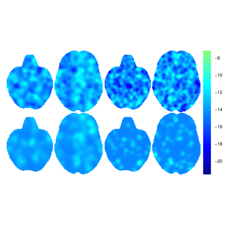
Figure 8: Some true (top row) and estimated (bottom row) latent Gaussian processes for type 1 (columns 1 and 2) and type 2 (columns 3 and 4) in the simulation setup 1 of Section B.1. Columns 1 and 3 correspond to axial slice $z=-22$; columns 2 and 4 correspond to axial slice $z=4$. While they may appear dissimilar at first, observe that the most intense regions of the true and estimated intensity match up; in this punishingly sparse setting (mean $\approx$ 4 foci per 3D image), the less intense regions have too few points to learn the intensity.

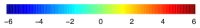
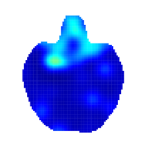
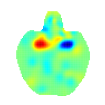
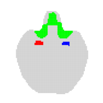
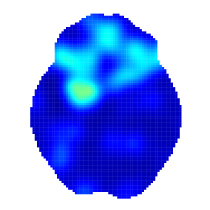
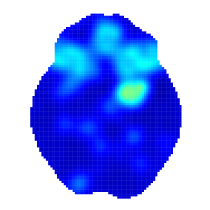
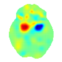
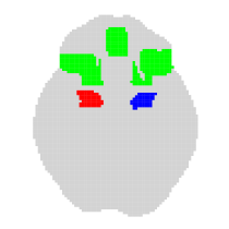
Figure 9: Results for simulation setup 2 of Section B.2. The top row corresponds to axial slice $z=-24$ whereas the bottom row corresponds to axial slice $z=-16$. Columns 1 and 2 are the estimated log-intensities for type 1 and type 2 respectively. The third column is the standardised mean posterior difference between the two latent Gaussian processes in the corresponding slice; bright colours indicate areas mostly activated by type 1 process. The fourth column shows the regions of the brain systematically activated by the two processes; red for type 1, blue for type 2 and green for both.

Appendix C Analysis of the WM dataset: supplementary plots

This section contains MCMC convergence diagnostics and supplemental material for the real data analysis of Section 5. Posterior traceplots are shown in Figures 10, 11, 12 and 13. The posterior traceplots for the marginal standard deviation parameters $\sigma_{k}$ and the correlation decay parameters $\rho_{k}$ are shown in Figure 10 (top and bottom row, respectively). Figure 11 shows posterior traceplots for the overall mean parameters $\mu_{k}$ (top row), the regression coefficient of the sample size covariate (bottom row, first subplot) and the integrated intensities of verbal and non-verbal studies (bottom row, second and third subplot, respectively). Let $v_{k}^{m}$ and $v_{k}^{M}$ be the voxels where the $k$-th latent GP $\boldsymbol{\beta}_{k}$ has the minimum and maximum mean posterior values, respectively. Posterior traceplots of $\left(\boldsymbol{\beta}_{0}\right)_{v_{0}^{m}}$, $\left(\boldsymbol{\beta}_{0}\right)_{v_{0}^{M}}$, $\left(\boldsymbol{\beta}_{1}\right)_{v_{1}^{m}}$, $\left(\boldsymbol{\beta}_{1}\right)_{v_{1}^{M}}$, $\left(\boldsymbol{\beta}_{2}\right)_{v_{2}^{m}}$ and $\left(\boldsymbol{\beta}_{2}\right)_{v_{2}^{M}}$ are shown in Figure 12. Finally, in Figure 13 we present $\alpha_{m}$ and $\alpha_{M}$, where $m$ and $M$ index the studies with the lowest and largest mean posterior random effects, respectively. All chains are obtained after applying a thinning factor of 15 to the original MCMC chains of length 15,000. Finally, Figure 14 shows the voxelwise posterior variance of $\exp{\left\{\boldsymbol{\beta}_{2}\right\}}$, the multiplicative age effect on the intensity of both verbal and non-verbal studies.

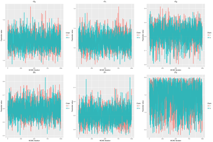
Figure 10: Posterior traceplots for some of the scalar parameters of the LGCP model of Equation 10 that we fit to the working memory dataset presented in Section 2. Top row: marginal standard deviations $\sigma_{k}$ of the 3 latent GPs. Bottom row: correlation decay parameters $\rho_{k}$ of the 3 latent GPs. The chains have been obtained after applying a thinning factor of 15 to the original chains of length 15,000.

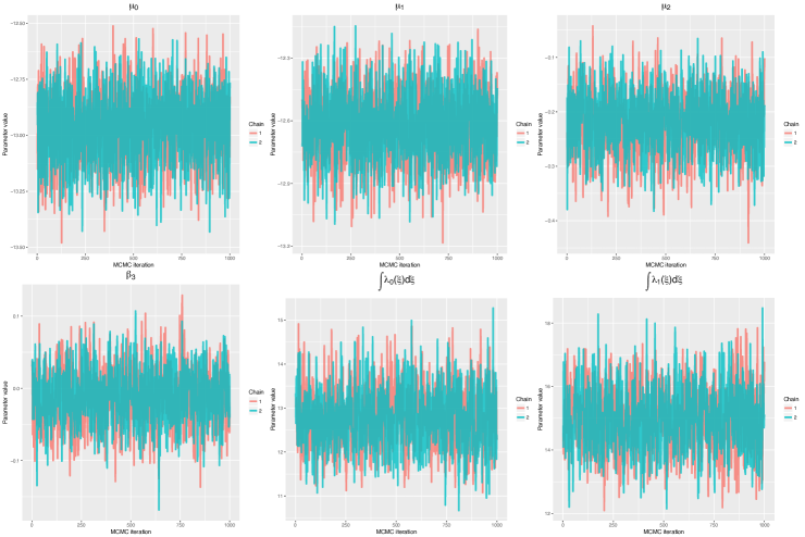
Figure 11: Posterior traceplots for some of the scalar parameters of the LGCP model of Equation 10 that we fit to the working memory dataset presented in Section 2. Top row: overall means $\mu_{k}$ of the 3 latent GPs. Bottom row, subplot 1: regression coefficient $\beta_{3}$ for the sample size covariate. Bottom row, subplots 2-3: integrated intensities for verbal and non-verbal studies, respectively. The chains have been obtained after applying a thinning factor of 15 to the original chains of length 15,000.

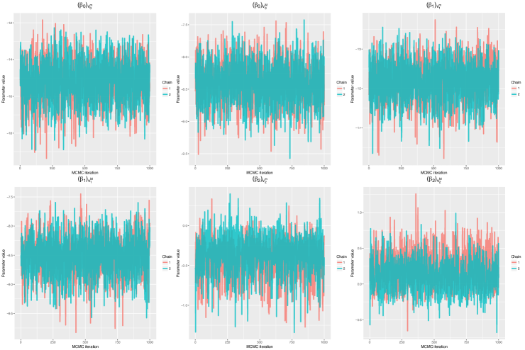
Figure 12: Posterior traceplots for some of the scalar parameters of the LGCP model of Equation 10 that we fit to the working memory dataset presented in Section 2. Subplots 1-6 correspond to $\left(\boldsymbol{\beta}_{0}\right)_{v_{0}^{m}}$, $\left(\boldsymbol{\beta}_{0}\right)_{v_{0}^{M}}$, $\left(\boldsymbol{\beta}_{1}\right)_{v_{1}^{m}}$, $\left(\boldsymbol{\beta}_{1}\right)_{v_{1}^{M}}$, $\left(\boldsymbol{\beta}_{2}\right)_{v_{2}^{m}}$ and $\left(\boldsymbol{\beta}_{2}\right)_{v_{2}^{M}}$, where $v_{k}^{m}$ and $v_{k}^{M}$ represent the voxels with the minimum and maximum mean posterior values of $\boldsymbol{\beta}_{k}$, respectively. The chains have been obtained after applying a thinning factor of 15 to the original chains of length 15,000.

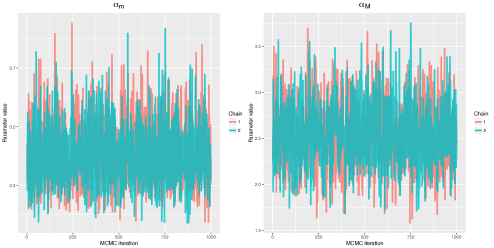
Figure 13: Posterior traceplots for some of the scalar parameters of the LGCP model of Equation 10 that we fit to the working memory dataset presented in Section 2. Subplots 1-2 represent $\alpha_{m}$ and $\alpha_{M}$, where $m$ and $M$ index the studies with the lowest and largest mean posterior random effects, respectively. The chains have been obtained after applying a thinning factor of 15 to the original chains of length 15,000.

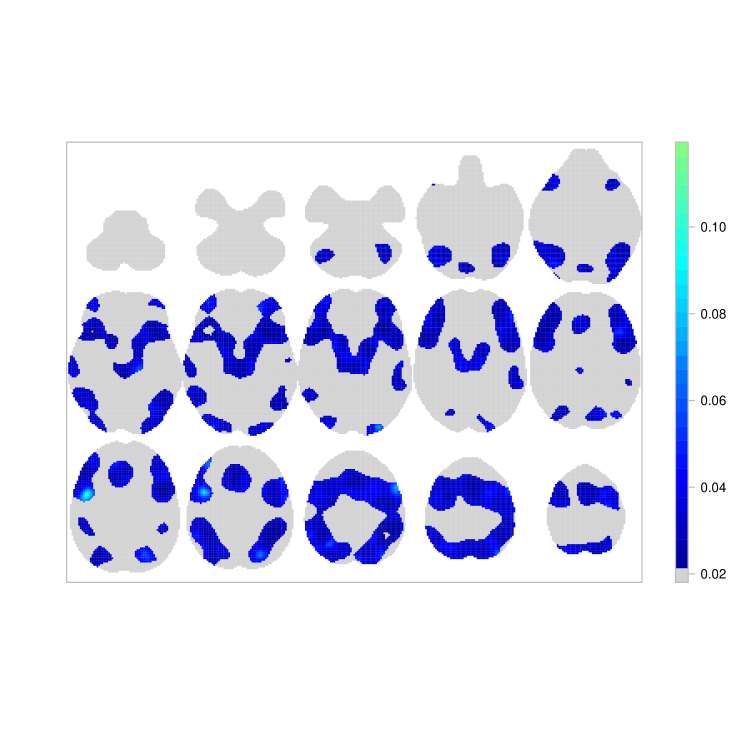
Figure 14: Posterior variance of $\exp{\left\{\boldsymbol{\beta}_{2}\right\}}$, the multiplicative age effect on the intensity of both verbal and non-verbal studies. Top row shows (from left to right) axial slices $z=-50,-42,-34,-26$ and $-18$, respectively. Middle row shows axial slices $z=-10,-2,+6,+14$ and $+22$, respectively. Bottom row shows axial slices $z=+30,+38,+46,+54$ and $+62$, respectively. Voxels for which the mean posterior $\boldsymbol{\lambda}$ is low (below the 75% quantile over the brain) have been set to zero.

Appendix D Full brain analysis

In this section we present full brain results for the working memory CBMA conducted in Section 5. Table LABEL:tab:fullbrain presents probabilities of activation and expected number of foci for several ROIs, along with their 95% credible intervals. In Table LABEL:tab:fullbrain2 we compare the probability of an activation between working memory studies using verbal and non-verbal stimuli, using the same ROIs. The ROIs have been obtained from the Harvard-Oxford atlas (Desikan et al., 2006). All quantities are based on 1,000 MCMC samples which are obtained after applying a thinning factor of 15 to the original MCMC chains of length 15,000.

Table 4: Working memory CBMA results. Table presents posterior summaries for the % probability of at least one activation in a given ROI (rounded to 2 decimal points), as well as the expected number of foci (rounded to 3 decimal points). All quantities have been calculated based on 1,000 MCMC samples.

		$\mathbf{\mathbb{P}\left(N_{X}(B)\geq 1\right)}$			$\mathbf{\int_{B}\lambda(\xi)d\xi}$
ROI	Vol.	Mean	$\mathbf{p_{0.025}}$	$\mathbf{p_{0.975}}$	Mean	$\mathbf{p_{0.025}}$	$\mathbf{p_{0.975}}$
Frontal pole	25900	60.24	51.05	66.42	0.926	0.714	1.091
Insular cortex	3613	33.39	26.68	39.36	0.407	0.310	0.500
Superior frontal gyrus	8861	38.27	27.74	43.98	0.484	0.325	0.579
Middle frontal gyrus	8421	60.55	48.23	66.48	0.933	0.658	1.093
Inferior frontal gyrus, pars triangularis	2317	22.54	15.44	27.94	0.256	0.168	0.328
Inferior frontal gyrus, pars opercularis	2335	39.88	31.06	45.96	0.510	0.372	0.615
Precentral gyrus	13967	68.47	59.96	73.72	1.158	0.915	1.336
Temporal pole	8044	9.60	5.41	13.48	0.101	0.056	0.145
Superior temporal gyrus, anterior division	916	1.77	0.80	2.87	0.018	0.008	0.029
Superior temporal gyrus, posterior division	2897	8.89	5.46	11.91	0.093	0.056	0.127
Middle temporal gyrus, anterior division	1425	1.64	0.55	2.88	0.017	0.005	0.029
Middle temporal gyrus, posterior division	4206	9.37	5.18	12.76	0.099	0.053	0.137
Middle temporal gyrus, temporooccipital part	3202	12.84	6.85	17.63	0.138	0.071	0.194
Inferior temporal gyrus, anterior division	1287	1.38	0.38	2.56	0.014	0.004	0.026
Inferior temporal gyrus, posterior division	4138	5.43	2.80	8.12	0.056	0.028	0.085
Inferior temporal gyrus, temporooccipital part	2605	11.49	6.16	16.05	0.122	0.064	0.175
Postcentral gyrus	10638	24.29	17.60	29.24	0.279	0.194	0.346
Superior parietal lobule	4489	36.16	26.16	42.31	0.450	0.303	0.550
Supramarginal gyrus, anterior division	2910	13.19	7.98	17.24	0.142	0.083	0.189
Supramarginal gyrus, posterior division	4071	28.38	19.69	33.72	0.335	0.219	0.411
Angular gyrus	3703	21.69	14.39	26.34	0.245	0.155	0.306
Lateral occipital cortex, superior division	14484	61.52	53.01	67.73	0.959	0.755	1.131
Lateral occipital cortex, inferior division	7490	27.53	18.66	33.57	0.323	0.207	0.409
Intracalcarine cortex	2211	8.36	4.35	11.76	0.087	0.045	0.125
Frontal medial cortex	1539	1.94	0.64	3.62	0.020	0.006	0.037
Juxtapositional lobule cortex	2282	26.46	16.14	32.74	0.308	0.176	0.397
Subcallosal cortex	2176	4.47	1.73	7.16	0.046	0.017	0.074
Paracingulate gyrus	4095	46.22	35.94	52.89	0.622	0.445	0.753
Cingulate gyrus, anterior division	4144	22.61	14.76	28.19	0.257	0.160	0.331
Cingulate gyrus, posterior division	4668	11.07	5.70	15.52	0.118	0.059	0.169
Precuneous cortex	7844	26.46	18.08	32.62	0.308	0.199	0.395
Cuneal cortex	1743	7.75	4.09	10.95	0.081	0.042	0.116
Frontal orbital cortex	5188	36.94	27.27	43.06	0.462	0.318	0.563
Parahippocampal gyrus, anterior division	3313	5.69	2.94	8.43	0.059	0.030	0.088
Parahippocampal gyrus, posterior division	2014	6.01	3.23	8.71	0.062	0.033	0.091
Lingual gyrus	5388	15.62	9.12	20.15	0.170	0.096	0.225
Temporal fusiform cortex, anterior division	1243	1.21	0.39	2.22	0.012	0.004	0.022
Temporal fusiform cortex, posterior division	2951	5.72	3.10	8.42	0.059	0.032	0.088
Temporal occipital fusiform cortex	2458	13.65	8.21	17.69	0.147	0.086	0.195
Occipital fusiform gyrus	3587	23.35	15.64	28.33	0.266	0.170	0.333
Frontal operculum cortex	1062	16.48	9.97	20.60	0.180	0.105	0.231
Central opercular cortex	2578	11.08	6.70	14.67	0.118	0.069	0.159
Parietal operculum cortex	1684	6.23	3.23	8.92	0.064	0.033	0.093
Planum polare	1210	2.64	1.29	3.94	0.027	0.013	0.040
Heschl’s gyrus	786	2.51	1.08	3.89	0.025	0.011	0.040
Planum temporale	1442	6.05	3.26	8.45	0.063	0.033	0.088
Supracalcarine cortex	424	1.52	0.66	2.41	0.015	0.007	0.024
Occipital pole	9658	20.42	12.04	25.75	0.229	0.128	0.298
Left cerebral white matter	28034	81.33	75.05	85.13	1.684	1.388	1.906
Left cerebral cortex	82249	99.04	98.05	99.44	4.679	3.938	5.193
Left lateral ventricle	1289	4.10	1.96	6.02	0.042	0.020	0.062
Left thalamus	1591	16.17	9.31	21.64	0.177	0.098	0.244
Left caudate	572	3.60	1.75	5.44	0.037	0.018	0.056
Left putamen	923	7.83	3.91	10.96	0.082	0.040	0.116
Left pallidum	312	5.15	2.58	7.59	0.053	0.026	0.079
Brain stem	8078	13.45	7.80	18.29	0.145	0.081	0.202
Left hippocampus	921	3.38	1.21	5.37	0.034	0.012	0.055
Left amygdala	390	1.41	0.48	2.43	0.014	0.005	0.025
Left accumbens	111	0.88	0.26	1.57	0.009	0.003	0.016
Right cerebral white matter	31216	79.16	72.13	83.13	1.573	1.278	1.780
Right cerebral cortex	86480	98.78	97.36	99.24	4.431	3.636	4.874
Right lateral ventricle	1019	3.36	1.77	4.97	0.034	0.018	0.051
Right thalamus	1398	12.88	7.12	17.43	0.138	0.074	0.192
Right caudate	515	2.68	1.02	4.30	0.027	0.010	0.044
Right putamen	800	6.82	3.39	9.80	0.071	0.034	0.103
Right pallidum	266	3.24	1.08	5.19	0.033	0.011	0.053
Right hippocampus	772	1.78	0.67	2.99	0.018	0.007	0.030
Right amygdala	399	0.86	0.19	1.73	0.009	0.002	0.017
Right accumbens	86	0.64	0.15	1.26	0.006	0.001	0.013

Table 5: Working memory CBMA results. Table presents posterior summaries for the % probability of a reported activation in studies using verbal and non-verbal stimuli. All quantities have been calculated based on 1,000 MCMC samples.

		Verbal			Non-verbal
ROI	Vol.	Mean	$\mathbf{p_{0.025}}$	$\mathbf{p_{0.975}}$	Mean	$\mathbf{p_{0.025}}$	$\mathbf{p_{0.975}}$
Frontal pole	25900	59.99	46.81	67.86	60.24	41.75	69.92
Insular cortex	3613	32.79	21.14	40.70	33.86	20.43	43.28
Superior frontal gyrus	8861	29.45	18.36	36.70	45.87	29.60	54.29
Middle frontal gyrus	8421	53.05	42.42	60.85	66.66	50.91	74.55
Inferior frontal gyrus, pars triangularis	2317	19.43	10.84	24.95	25.44	14.64	33.90
Inferior frontal gyrus, pars opercularis	2335	43.66	31.68	51.15	35.69	21.49	44.80
Precentral gyrus	13967	64.10	51.56	71.00	72.09	57.82	79.52
Temporal pole	8044	7.54	2.91	11.50	11.58	4.28	18.15
Superior temporal gyrus, anterior division	916	2.31	0.71	4.05	1.23	0.27	2.52
Superior temporal gyrus, posterior division	2897	10.76	5.31	15.14	6.95	2.25	11.32
Middle temporal gyrus, anterior division	1425	2.19	0.48	4.36	1.09	0.15	2.56
Middle temporal gyrus, posterior division	4206	9.58	4.59	14.22	9.12	3.83	14.44
Middle temporal gyrus, temporooccipital part	3202	11.88	5.65	17.75	13.73	5.73	21.06
Inferior temporal gyrus, anterior division	1287	1.76	0.31	3.69	0.99	0.10	2.53
Inferior temporal gyrus, posterior division	4138	4.85	1.59	8.09	5.98	1.47	10.31
Inferior temporal gyrus, temporooccipital part	2605	7.45	3.00	11.83	15.31	6.95	22.66
Postcentral gyrus	10638	20.37	11.48	26.10	27.95	16.64	35.68
Superior parietal lobule	4489	38.81	26.05	46.48	33.24	19.67	42.96
Supramarginal gyrus, anterior division	2910	12.78	5.90	17.83	13.56	6.23	19.83
Supramarginal gyrus, posterior division	4071	29.93	19.40	36.61	26.70	14.58	35.17
Angular gyrus	3703	24.30	15.51	31.09	18.91	9.32	25.61
Lateral occipital cortex, superior division	14484	55.45	42.51	63.87	66.55	52.60	74.58
Lateral occipital cortex, inferior division	7490	23.69	14.54	30.51	31.06	18.71	40.58
Intracalcarine cortex	2211	6.51	2.61	10.12	10.15	4.37	15.19
Frontal medial cortex	1539	1.21	0.24	2.62	2.66	0.60	5.58
Juxtapositional lobule cortex	2282	21.21	12.33	28.23	31.23	18.26	41.74
Subcallosal cortex	2176	4.20	1.08	7.66	4.72	1.03	9.24
Paracingulate gyrus	4095	42.91	29.21	51.04	49.14	33.89	59.57
Cingulate gyrus, anterior division	4144	17.69	10.95	24.25	27.15	14.86	36.16
Cingulate gyrus, posterior division	4668	8.06	3.60	12.42	13.93	5.98	21.66
Precuneous cortex	7844	22.88	12.61	30.03	29.76	18.38	39.96
Cuneal cortex	1743	6.71	1.97	10.43	8.76	3.29	14.54
Frontal orbital cortex	5188	37.26	25.37	45.24	36.48	24.30	45.43
Parahippocampal gyrus, anterior division	3313	5.93	2.24	9.59	5.44	1.65	9.35
Parahippocampal gyrus, posterior division	2014	5.80	2.27	9.47	6.21	2.46	10.81
Lingual gyrus	5388	15.61	7.56	21.30	15.56	7.52	22.72
Temporal fusiform cortex, anterior division	1243	1.52	0.33	3.13	0.90	0.18	2.11
Temporal fusiform cortex, posterior division	2951	5.26	2.06	8.46	6.17	2.13	10.49
Temporal occipital fusiform cortex	2458	8.87	4.19	13.17	18.12	8.94	26.00
Occipital fusiform gyrus	3587	26.68	17.03	33.74	19.78	10.47	27.65
Frontal operculum cortex	1062	15.27	9.08	20.31	17.64	9.10	23.87
Central opercular cortex	2578	10.04	4.95	14.41	12.08	5.64	17.46
Parietal operculum cortex	1684	7.35	2.65	11.29	5.08	1.56	9.05
Planum polare	1210	2.37	0.79	4.02	2.91	0.98	5.02
Heschl’s gyrus	786	3.07	0.99	5.47	1.94	0.34	3.79
Planum temporale	1442	7.38	3.50	10.90	4.69	1.55	8.26
Supracalcarine cortex	424	0.95	0.29	1.74	2.07	0.51	3.64
Occipital pole	9658	19.84	10.66	26.91	20.91	11.10	29.20
Left cerebral white matter	28034	76.33	66.31	81.39	85.13	75.35	89.94
Left cerebral cortex	82249	98.88	97.31	99.41	99.14	97.59	99.63
Left lateral ventricle	1289	3.12	1.30	5.16	5.05	1.65	8.64
Left thalamus	1591	14.56	7.44	20.87	17.69	7.35	26.38
Left caudate	572	3.49	1.25	5.71	3.69	1.09	6.53
Left putamen	923	6.97	2.01	11.15	8.67	2.25	13.88
Left pallidum	312	6.26	2.38	10.29	4.01	1.24	7.29
Brain stem	8078	10.42	5.26	15.72	16.33	6.90	25.06
Left hippocampus	921	3.46	1.08	6.28	3.29	0.74	6.39
Left amygdala	390	1.21	0.16	2.59	1.60	0.25	3.37
Left accumbens	111	1.07	0.15	2.29	0.69	0.09	1.49
Right cerebral white matter	31216	73.44	65.11	78.96	83.50	74.00	88.46
Right cerebral cortex	86480	98.22	96.50	98.97	99.12	97.60	99.61
Right lateral ventricle	1019	2.66	0.96	4.35	4.05	1.21	6.74
Right thalamus	1398	15.17	8.00	21.79	10.48	3.36	16.86
Right caudate	515	2.51	0.76	4.45	2.85	0.68	5.34
Right putamen	800	5.91	1.94	9.49	7.69	2.56	12.98
Right pallidum	266	2.74	0.65	4.97	3.73	0.93	6.91
Right hippocampus	772	1.77	0.52	3.42	1.78	0.46	3.55
Right amygdala	399	0.86	0.11	2.03	0.87	0.13	2.17
Right accumbens	86	0.78	0.13	1.84	0.50	0.08	1.30

References

- Benes et al. (2002) Benes, V., Bodlák, K., Møller, J., and Waagepetersen, R. P. (2002). Bayesian analysis of log Gaussian Cox processes for disease mapping. Technical report, Depertment of Mathematical Sciences, Aalborg University.
- Christensen and Waagepetersen (2002) Christensen, O. F. and Waagepetersen, R. P. (2002). Bayesian prediction of spatial count data using generalized linear mixed models. Biometrics, 58(2), 280–286.
- Christensen et al. (2006) Christensen, O. F., Roberts, G. O., and Sköld, M. (2006). Robust Markov chain Monte Carlo methods for spatial generalized linear mixed models. Journal of Computational and Graphical Statistics, 15(1), 1–17.
- Desikan et al. (2006) Desikan, R. S., Ségonne, F., Fischl, B., Quinn, B. T., Dickerson, B. C., Blacker, D., Buckner, R. L., Dale, A. M., Maguire, R. P., Hyman, B. T., Albert, M. S., and Killiany, R. J. (2006). An automated labeling system for subdividing the human cerebral cortex on MRI scans into gyral based regions of interest. NeuroImage, 31(3), 968–980.
- Dietrich and Newsam (1993) Dietrich, C. R. and Newsam, G. N. (1993). A fast and exact method for multidimensional Gaussian stochastic simulations. Water Resources Research, 29(8), 2861–2869.
- Diggle et al. (2013) Diggle, P. J., Moraga, P., Rowlingson, B., and Taylor, B. M. (2013). Spatial and spatio-temporal log-Gaussian Cox processes: Extending the geostatistical paradigm. Statistical Science, 28(4), 542–563.
- Duane et al. (1987) Duane, S., Kennedy, A. D., Pendleton, B. J., and Roweth, D. (1987). Hybrid Monte Carlo. Physics Letters B, 195(2), 216–222.
- Eickhoff et al. (2012) Eickhoff, S. B., Bzdok, D., Laird, A. R., Kurth, F., and Fox, P. T. (2012). Activation likelihood estimation meta-analysis revisited. NeuroImage, 59(3), 2349–2361.
- Gelman et al. (1996) Gelman, A., Meng, X.-L., and Stern, H. (1996). Posterior predictive assessment of model fitness via realized discrepancies. Statistica Sinica, 6(4), 733–807.
- Girolami and Calderhead (2011) Girolami, M. and Calderhead, B. (2011). Riemann manifold Langevin and Hamiltonian Monte Carlo methods. Journal of the Royal Statistical Society, Series B: Statistical Methodology, 73(2), 123–214.
- Gneiting and Raftery (2007) Gneiting, T. and Raftery, A. E. (2007). Strictly proper scoring rules, prediction, and estimation. Journal of the American Statistical Association, 102(477), 359–378.
- Greenland (1994) Greenland, S. (1994). Invited commentary: a critical look at some popular meta-analytic methods. American Journal of Epidemiology, 140(3), 290–296.
- Hartung et al. (2008) Hartung, J., Knapp, G., and Sinha, B. K. (2008). Statistical Meta-Analysis with Applications. John Wiley & Sons, Hoboken.
- Hoffman and Gelman (2014) Hoffman, M. and Gelman, A. (2014). The No-U-turn sampler: adaptively setting path lengths in Hamiltonian Monte Carlo. Journal of Machine Learning Research, 15(1), 1593–1623.
- Illian et al. (2012a) Illian, J. B., Sørbye, S. H., and Rue, H. (2012a). A toolbox for fitting complex spatial point process models using integrated nested Laplace approximation (INLA). The Annals of Applied Statistics, 6(4), 1499–1530.
- Illian et al. (2012b) Illian, J. B., Sørbye, S. H., Rue, H., and Hendrichsen, D. K. (2012b). Using INLA to fit a complex point process model with temporally varying effects – A case study. Journal of Environmental Statistics, 3(7), 1–25.
- Jaakkola and Jordan (2000) Jaakkola, T. and Jordan, M. (2000). Bayesian parameter estimation via variational methods. Statistics and Computing, 10(1), 25–37.
- Kang et al. (2011) Kang, J., Johnson, T. D., Nichols, T. E., and Wager, T. D. (2011). Meta analysis of functional neuroimaging data via Bayesian spatial point processes. Journal of the American Statistical Association, 106(493), 124–134.
- Kang et al. (2014) Kang, J., Nichols, T. E., Wager, T. D., and Johnson, T. D. (2014). A Bayesian hierarchical spatial point process model for multi-type neuroimaging meta-analysis. The Annals of Applied Statistics, 8(3), 1561–1582.
- Laird et al. (2005) Laird, A. R., Lancaster, J. J., and Fox, P. T. (2005). Brainmap: the social evolution of a human brain mapping database. Neuroinformatics, 3(1), 65–77.
- Leininger and Gelfand (2017) Leininger, T. J. and Gelfand, A. E. (2017). Bayesian inference and model assessment for spatial point patterns using posterior predictive samples. Bayesian Analysis, 12(1), 1–30.
- Liang et al. (2009) Liang, S., Carlin, B. P., and Gelfand, A. E. (2009). Analysis of Minnesota colon and rectum cancer point patterns with spatial and nonspatial covariate information. The Annals of Applied Statistics, 3(3), 943–962.
- Marshall and Roberts (2012) Marshall, T. and Roberts, G. (2012). An adaptive approach to Langevin MCMC. Statistics and Computing, 22(5), 1041–1057.
- Møller and Waagepetersen (2003) Møller, J. and Waagepetersen, R. P. (2003). An introduction to simulation-based inference for spatial point processes. In J. Møller, editor, Spatial Statistics and Computational Methods, chapter 4, pages 143–198. Springer-Verlag.
- Møller and Waagepetersen (2004) Møller, J. and Waagepetersen, R. P. (2004). Statistical Inference and Simulation for Spatial Point Processes. Chapman and Hall/CRC, Boca Raton.
- Møller and Waagepetersen (2007) Møller, J. and Waagepetersen, R. P. (2007). Modern statistics for spatial point processes. Scandinavian Journal of Statistics, 34(4), 643–684.
- Møller et al. (1998) Møller, J., Syversveen, A. R., and Waagepetersen, R. P. (1998). Log Gaussian Cox processes. Scandinavian Journal of Statistics, 25(3), 451–482.
- Montagna et al. (2017) Montagna, S., Wager, T., Barrett, L. F., Johnson, T. D., and Nichols, T. E. (2017). Spatial bayesian latent factor regression modeling of coordinate-based meta-analysis data. Biometrics.
- Murray et al. (2010) Murray, I., Adams, R. P., and MacKay, D. J. (2010). Elliptical slice sampling. Journal of Machine Learning Research: Workshop and Conference Proceeding, 9(6), 541–548.
- Neal (1996) Neal, R. M. (1996). Bayesian Learning for Neural Networks. Springer-Verlag New York, Inc., Secaucus, NJ, USA.
- Neal (2011) Neal, R. M. (2011). MCMC using Hamiltonian dynamics. In S. Brooks, A. Gelman, G. L. Jones, and X. Meng, editors, Handbook of Markov Chain Mote Carlo, chapter 5, pages 113–162. Chapman & Hall/CRC.
- Owen et al. (2005) Owen, A. M., McMillan, K. M., Laird, A. R., and Bullmore, E. (2005). N-back working memory paradigm: A meta-analysis of normative functional neuroimaging studies. Human brain mapping, 25(1), 46–59.
- Park and van Dyk (2009) Park, T. and van Dyk, D. A. (2009). Partially collapsed gibbs samplers: Illustrations and applications. Journal of Computational and Graphical Statistics, 18(2), 283–305.
- Radua and Mataix-Cols (2009) Radua, J. and Mataix-Cols, D. (2009). Voxel-wise meta-analysis of grey matter changes in obsessive-compulsive disorder. The British Journal of Psychiatry : the Journal of Mental Science, 195(5), 393–402.
- Radua et al. (2012) Radua, J., Mataix-Cols, D., Phillips, M. L., El-Hage, W., Kronhaus, D. M., Cardoner, N., and Surguladze, S. (2012). A new meta-analytic method for neuroimaging studies that combines reported peak coordinates and statistical parametric maps. European Psychiatry, 27(8), 605–611.
- Rasmussen and Williams (2005) Rasmussen, C. E. and Williams, C. K. I. (2005). Gaussian Processes for Machine Learning (Adaptive Computation and Machine Learning). The MIT Press.
- Rottschy et al. (2012) Rottschy, C., Langner, R., Dogan, I., Reetz, K., Laird, A. R., Schulz, J. B., Fox, P. T., and Eickhoff, S. B. (2012). Modelling neural correlates of working memory: a coordinate-based meta-analysis. NeuroImage, 60(1), 830–846.
- Rue and Held (2005) Rue, H. and Held, L. (2005). Gaussian Markov Random Fields: Theory and Applications. Chapman & Hall/CRC Monographs on Statistics & Applied Probability. Taylor & Francis.
- Salimi-Khorshidi et al. (2009) Salimi-Khorshidi, G., Smith, S. M., Keltner, J. R., Wager, T. D., and Nichols, T. E. (2009). Meta-analysis of neuroimaging data: a comparison of image-based and coordinate-based pooling of studies. NeuroImage, 45(3), 810–823.
- Samartsidis et al. (2017) Samartsidis, P., Montagna, S., Laird, A. R., Fox, P. T., Johnson, T. D., and Nichols, T. E. (2017). Estimating the number of missing experiments in a neuroimaging meta-analysis. bioRxiv, page 225425.
- Simpson et al. (2016) Simpson, D., Illian, J., Lindgren, F., Sørbye, S., and Rue, H. (2016). Going off grid: computationally efficient inference for log-Gaussian Cox processes. Biometrika, 103(1), 49–70.
- Taylor and Diggle (2014) Taylor, B. M. and Diggle, P. J. (2014). INLA or MCMC? A tutorial and comparative evaluation for spatial prediction in log-Gaussian Cox processes. Journal of Statistical Computation and Simulation, 84(10), 2266–2284.
- Turkeltaub et al. (2002) Turkeltaub, P. E., Eden, G. F., Jones, K. M., and Zeffiro, T. A. (2002). Meta-analysis of the functional neuroanatomy of single-word reading: method and validation. NeuroImage, 16(3, Part A), 765–780.
- Waagepetersen (2004) Waagepetersen, R. P. (2004). Convergence of posteriors for discretized log Gaussian Cox processes. Statistics and Probability Letters, 66(3), 229–235.
- Wager et al. (2003) Wager, T. D., Phan, K., Liberzon, I., and Taylor, S. F. (2003). Valence, gender, and lateralization of functional brain anatomy in emotion: a meta-analysis of findings from neuroimaging. NeuroImage, 19(3), 513–531.
- Wager et al. (2004) Wager, T. D., Jonides, J., and Reading, S. (2004). Neuroimaging studies of shifting attention: a meta-analysis. NeuroImage, 22(4), 1679–1693.
- Wager et al. (2007) Wager, T. D., Lindquist, M., and Kaplan, L. (2007). Meta-analysis of functional neuroimaging data: current and future directions. Social Cognitive and Affective Neuroscience, 2(2), 150–158.
- Wood and Chan (1994) Wood, A. T. A. and Chan, G. (1994). Simulation of stationary Gaussian processes in . Journal of Computational and Graphical Statistics, 3(4), 409–432.
- Yue et al. (2012) Yue, Y. R., Lindquist, M. A., and Loh, J. M. (2012). Meta-analysis of functional neuroimaging data using Bayesian nonparametric binary regression. The Annals of Applied Statistics, 6(2), 697–718.
- Zhang (2004) Zhang, H. (2004). Inconsistent estimation and asymptotically equal interpolations in model-based geostatistics. Journal of the American Statistical Association, 99(465), 250–261.