Active cluster crystals

Abstract

We study the appearance and properties of cluster crystals (solids in which the unit cell is occupied by a cluster of particles) in a two-dimensional system of self-propelled active Brownian particles with repulsive interactions. Self-propulsion deforms the clusters by depleting particle density inside, and for large speeds it melts the crystal. Continuous field descriptions at several levels of approximation allow to identify the relevant physical mechanisms.

I Introduction

The collective behavior of self-propelled particles is a fascinating topic both for its numerous applications and its intrinsic theoretical interest Ramaswamy (2010); Cates et al. (2010); Marchetti et al. (2013); Romanczuk et al. (2012). Many studies focused on the formation of clusters reporting two main different cases: for “active crystals”, self-propulsion leads to a modification of the properties of a pre-existing crystal that is usually induced by long-range attractive and short-range repulsive interactions Mani and Löwen (2015); Menzel et al. (2014); Menzel and Löwen (2013). On the other hand, for Mobility-Induced Phase Separation (MIPS), the system separates into two fluid phases of different densities. Clusters of the densest phase form by a purely non-equilibrium mechanism induced by the persistence of the motion of the particles, the nature of their interactions being not as crucial (this phenomenon was observed for various repulsive and attractive forces Cates and Tailleur (2015); Mognetti et al. (2013); Redner et al. (2013)). Methodologically, both mechanisms can be studied by considering an effective density-dependent velocity replacing the two-body interacting potential Tailleur and Cates (2008); Fily and Marchetti (2012); Farrell et al. (2012); Cates and Tailleur (2013); Stenhammar et al. (2013); Bialké et al. (2013); Fily et al. (2014).

We analyze in this paper a different case of cluster formation with active objects (some additional models and experiments on clustering of self-propelled particles maybe found, for example, in Buttinoni et al. (2013); Redner et al. (2013); Theurkauff et al. (2012)). It is the non-equilibrium counterpart of the so-called cluster crystals Klein et al. (1994); Likos et al. (2001); Mladek et al. (2006); Likos et al. (2007); Mladek et al. (2008); Coslovich and Ikeda (2013), which appear in equilibrium systems interacting with soft-core repulsive potentials, and are solid-like structures where the unit cell is occupied by a closely packed cluster of particles. Here, clustering appears under a repulsive potential so that it is not a consequence of purely local effects but rather involves a global minimization of energy by intercluster interactions. Namely, for sufficiently soft repulsive potentials, repulsion from the neighboring clusters can exceed the intracluster repulsion and lead to an effective particle confinement in the cluster. For the active-particle case discussed here, this mechanism is very different from the other cases of active crystals and it is unlikely that previous local arguments derived for active crystals or MIPS can describe it.

Similarly to previous works Menzel et al. (2014); Mani and Löwen (2015), we consider the simplest extension of an equilibrium system of repulsive Brownian particles in two dimensions by providing them with an internal degree-of-freedom, the orientation of a self-propulsion speed. We will address the following questions: Do active cluster crystals (ACC) with only repulsive interactions exist? Is the structure of the clusters modified by activity? Can we find continuum equations describing this active system? The answer to the first question has been partially given by observations of cluster crystals in Menzel and Ohta (2012); Menzel (2013), for example. But in these references the focus is in deformable-body and alignment interactions, so that the specific role of repulsive interactions needs further clarification.

To do this and answer the remaining questions we first present numerical simulations of self-propelled soft repulsive particles showing that ACC can be observed but that an increasing self-propulsion eventually leads to their destruction. For small diffusion, empty clusters are found as the particles tend to accumulate on their edges. Then we provide a continuum field description of this interacting particle system and analyze some of its predictions.

II Numerical results and pattern formation

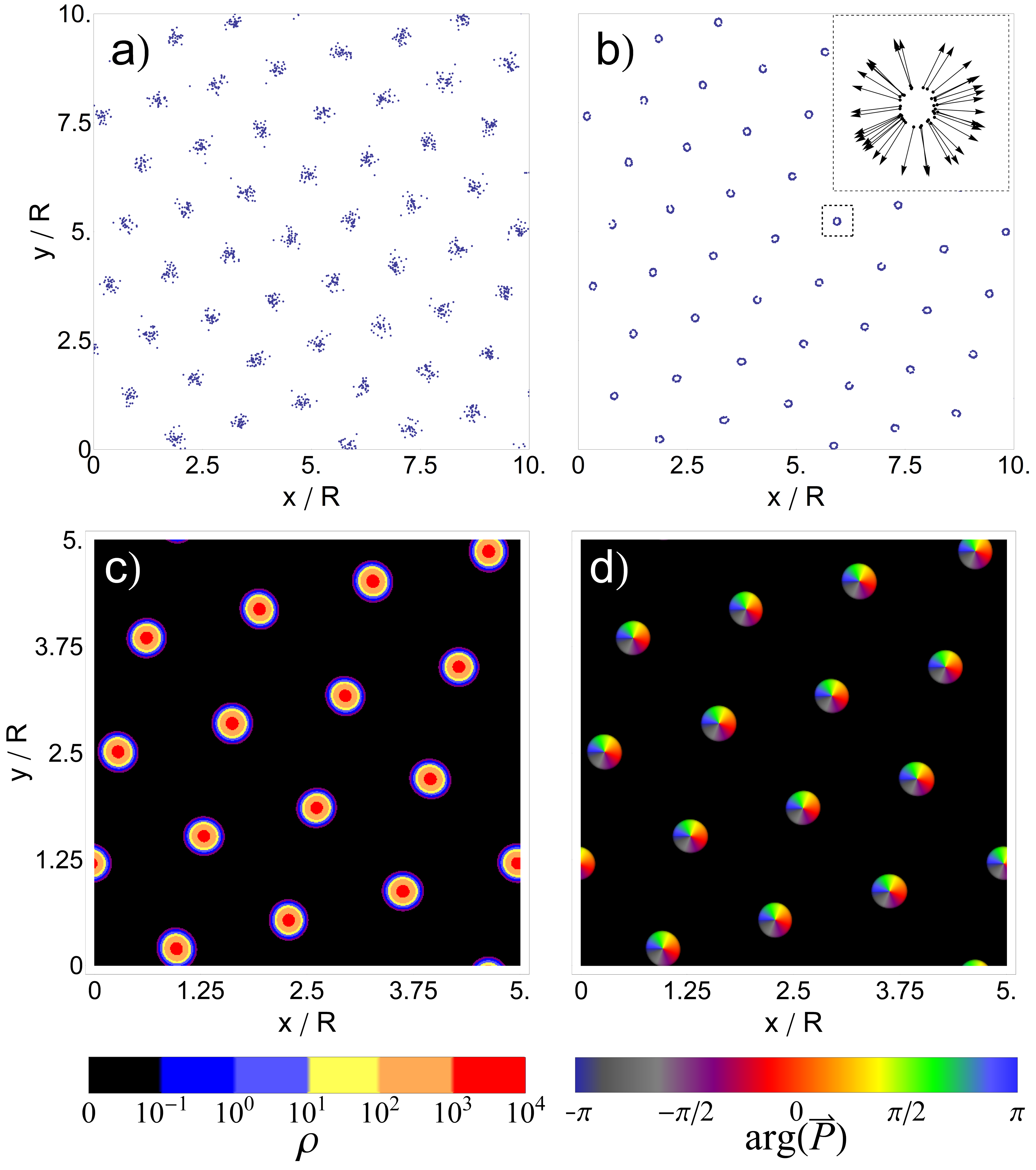
Figure 1: a) and b) Particle simulations: snapshots of the positions of the particles in the steady-state for $\bar{\rho}=2000$, $L=1$, $D_{r}=0.1$ and a GEM-3 potential with $R=0.1$ and $\epsilon=0.0333$. a) $D=3\times 10^{-2}$, $U_{0}=1.0$. b) $D=10^{-4}$ , $U_{0}=3.0$. The top-right inset is a zoom of the boxed cluster showing the orientation vector ${\boldsymbol{\hat{n}}}$ of the particles inside it. c) and d) Steady-states obtained by numerical integration of Eqs. (10). Same parameters as in panel a) except $L=0.5$. c) Local density $\rho$ . d) Orientation angle $\arg\boldsymbol{P}$ of the polarization field, encoded in colors. The modulus $|\boldsymbol{P}|$ is encoded in the opacity, so that the black areas correspond to very small polarizations.

We start with the Langevin equations of a two-dimensional overdamped system of active Brownian particles interacting in pairs via a potential $V({\bf x})$:

$$\dot{\bf x}_{i}(t) = U_{0}{\boldsymbol{\hat{n}}}(\theta_{i}(t))-\sum_{j\neq i}\nabla V({\bf x}_{i}-{\bf x}_{j})+\sqrt{2D}{\boldsymbol{\xi}}_{i}(t),$$

$$\dot{\theta}_{i}(t) = \sqrt{2D_{r}}\xi_{i}^{r}(t)\ .$$ (1)

$\left(x_{i},y_{i}\right)={\bf x}_{i}$ and $\theta_{i}$ are respectively the position and orientation of the particle $i$, $U_{0}{\boldsymbol{\hat{n}}}$ is the self-propelling velocity, of constant modulus $U_{0}$ and direction given by the unit vector ${\boldsymbol{\hat{n}}}(\theta_{i})=(\cos\theta_{i},\sin\theta_{i})$. The particles are subjected to Gaussian translational and rotational noises, ${\boldsymbol{\xi}}_{i}=(\xi_{i}^{x},\xi_{i}^{y})$ and $\xi^{r}_{i}$ respectively, satisfying $\left<\xi_{i}^{\alpha}\right>=0$, and $\left<\xi^{\alpha}_{i}(t)\xi^{\beta}_{j}(t^{\prime})\right>=\delta_{ij}\delta_{\alpha\beta}\delta(t-t^{\prime})$, for $\alpha,\beta=x,y,r$. $D$ and $D_{r}$ are the translation and rotational diffusion coefficients. If they originate from the same thermal bath they are related to temperature by fluctuation-dissipation relationships. But under general non-equilibrium conditions they can have different origins and then we will assume here that they are independent parameters.

Cluster crystals appear at equilibrium ($U_{0}=0$) under repulsive soft-core potentials which have negative Fourier components Likos et al. (2007); Delfau et al. (2016). A convenient class of such potentials is the generalized exponential model of exponent $\alpha$ (GEM-$\alpha$): $V({\bf x})=\epsilon\exp\left(-\left|{\bf x}/{R}\right|^{\alpha}\right)$, $\epsilon>0$, and $R$ is the interaction range. The Fourier transform $\tilde{V}(q)$ of GEM-$\alpha$ potentials with $\alpha>2$ takes both positive and negative values, so that cluster crystals would appear in that case for sufficiently small $D$ Likos et al. (2007); Delfau et al. (2016) and/or large average densities $\bar{\rho}$. Here we consider $\alpha=3$.

Besides the global parameters $N$ and $L$, which fix the mean density $\bar{\rho}=N/L$, our model contains five parameters: $D$, $D_{r}$, $U_{0}$, and the two parameters in the potential ($\epsilon$ and $R$). By proper choosing of space and time units, all dependence in these five parameters gets condensed in a set of three dimensionless quantities, for which one of the possible choices is $U_{0}/\sqrt{D_{r}D}$, $\epsilon D_{r}/U_{0}^{2}$, and $D_{r}R/U_{0}$. The first parameter compares the strength of self-propulsion with that of translational diffusion, the second the strength of the interaction forces with self-propulsion, and the third the persistence length with the interaction length. Unless otherwise stated, in the following we will fix the parameters in the potential (to $\epsilon=0.0333$ and $R=0.1$) and $D_{r}=0.1$ (this last one being equivalent to fixing the units of time), and describe the behavior of the system by varying $U_{0}$ and $D$. Other ways to explore the transitions occurring in the system are possible, and they can be easily related to the one described here simply by looking at the dimensionless quantities stated above. For example, in the dimensionless parameters the dependence on $D_{r}$ is reciprocal to that on $U_{0}$, meaning that the changes in behavior described below when increasing $U_{0}$ at $D_{r}$ fixed will also be observed when decreasing $D_{r}$ at $U_{0}$ fixed.

We integrate numerically (II) with the Euler-Maruyama method Toral and Colet (2014). For small $U_{0}$ we observe a transition, when increasing the average density $\bar{\rho}$ or decreasing the diffusion coefficient $D$, from a homogeneous distribution of particles to a statistically steady hexagonal crystal of clusters (see figure 1 a,b), similar to the behavior observed for passive particles ($U_{0}=0$). If $U_{0}$ and $D$ are small enough, there is no particle exchange between clusters. If $U_{0}$ is further increased, the cluster crystal remains but jumps between clusters eventually occur. For high values of $U_{0}$ clusters are destroyed and the steady-state becomes statistically homogeneous (see Table 1 for precise values). Contrary to the passive case for which the distribution of particles inside a cluster is Gaussian to a good approximationDelfau et al. (2016), active particles tend to stay close to the edges. This is particularly obvious for small $D$ and high $U_{0}$. In that case, the clusters have a ring shape with their centers empty (see figure 1 b). We confirmed this by computing the distribution of $\Delta r$, the relative distance between the position of a particle and the center of its cluster. Figure 2 a) shows that when $U_{0}$ is large and $D$ small, there is a clear depletion close to $\Delta r=0$ while the distributions look Gaussian for higher $D$ (remember than the relevant dimensionless parameter is $U_{0}/\sqrt{D_{r}D}$, so that simple Gaussian clusters are also obtained for large enough $D_{r}$). A similar cluster-center depletion Nash et al. (2010); Menzel (2015); Menzel et al. (2016) has been observed in active systems in which aggregation occurs by confinement in an external potential. Our studies in Sect. III.2 below will show that indeed both phenomena are related. They arise from a purely non-equilibrium effect caused by the persistence of the particle velocity which disappears for small $U_{0}$ or large $D_{r}$. Another consequence of persistence is that the orientation ${\boldsymbol{\hat{n}}}$ of the particles inside a cluster is clearly radial, pointing to the exterior (inset of figure 1 b). For larger $D$ like in figure 1 a), this radial orientation of velocity vectors remains predominant but not as strong. From the definition of the model, and as we will show later on, the equilibrium Brownian non-active dynamics, for which clusters are no longer empty, is achieved for large $D_{r}$.

     

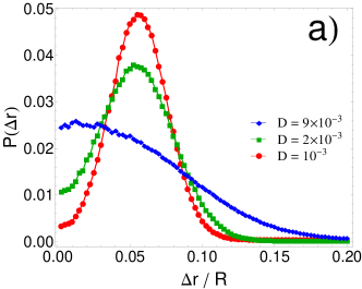
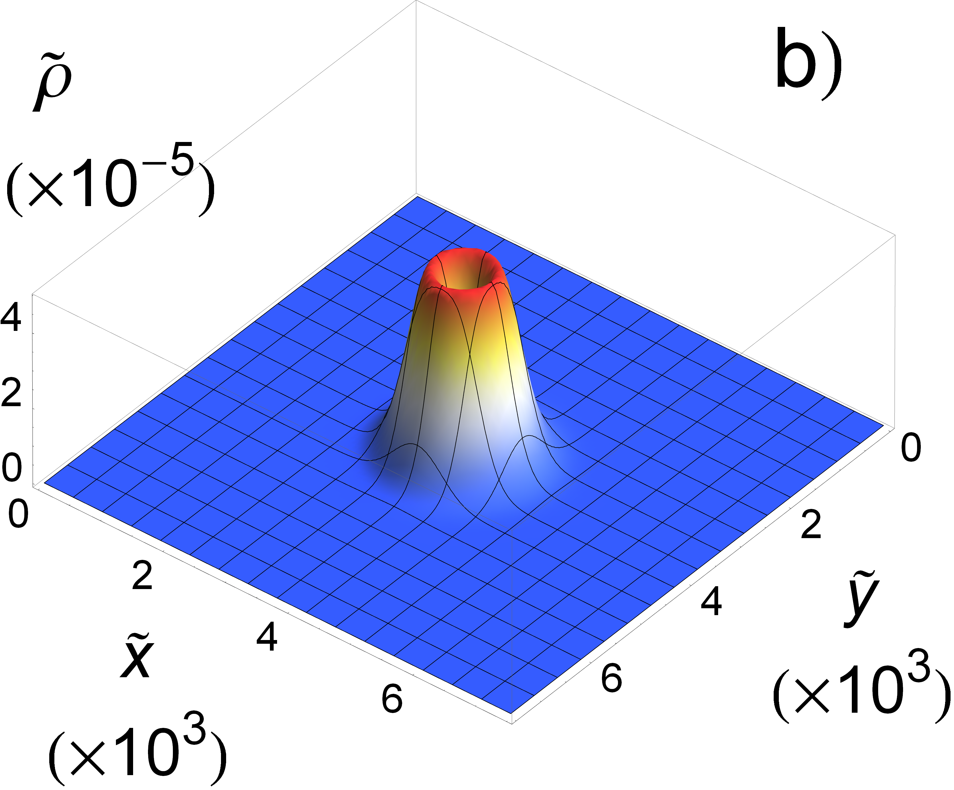
Figure 2: a) Probability of finding a particle at a distance $[\Delta r,\Delta r+dr]$ from the center of its cluster, normalized by $2\pi\Delta rdr$ to give an estimation of the particle density. Same parameters as in figure 1 a) and b) except $U_{0}=2.5$, and $D=10^{-3}$ (red disks), $2\times 10^{-3}$ (green squares), and $9\times 10^{-3}$ (blue diamonds). b) Steady-state solution of Eqs.(10) showing a 2D empty cluster. The interaction force $\boldsymbol{F}_{\rho}$ of Eqs.(10) was replaced by an effective confinement force $\boldsymbol{F}_{eff}=\left(\tilde{a}\sin(2\pi(\tilde{x}/\tilde{L}-0.5)),\tilde{a}\sin(2\pi(\tilde{y}/\tilde{L}-0.5))\right)$. The parameters have been nondimensionalized by $D_{r}$ and $U_{0}$ so that $\tilde{a}=a/U_{0}=2.5$, $\tilde{L}=LD_{r}/U_{0}=7.5\times 10^{-3}$, $\tilde{D}=DD_{r}/U_{0}^{2}=1.88\times 10^{-3}$. The integral of $\tilde{\rho}$ is equal to 1.

III Theoretical description: active Dean-Kawasaki equation

III.1 Derivation and stability analysis

To have some analytical handle on the phenomena above we derive now the equivalent of a Dean-Kawasaki (DK) equation Kawasaki (1994); Dean (1996); Delfau et al. (2016) for active particles. Note that a continuum description equivalent to the particle system should include a noise term arising from the random discrete particle dynamics. However, as in Delfau et al. (2016) we average out noise terms to obtain a deterministic version of the DK equation. To do so, we start from (II). The function $\hat{\rho}({\bf x},\theta,t)=\sum_{i}^{N}\delta({\bf x}-{\bf x}_{i}(t))\delta(\theta-\theta_{i}(t))$ is an Itō process so that we can apply the Itō formulaOksendal (2000). Using integration by parts we obtain the following deterministic equation for the average $\rho({\bf x},\theta,t)\equiv\left<\hat{\rho}({\bf x},\theta,t)\right>$, which is the expected value of the density of particles at location ${\bf x}$ and with orientation $\theta$:

$$\partial_{t}\rho({\bf x},\theta,t)=\nabla\cdot\left(\rho({\bf x},\theta,t)\int d{\bf x}^{\prime}\nabla V({\bf x}-{\bf x}^{\prime})\rho({\bf x}^{\prime},t)\,\right)$$

$$+D\nabla^{2}\rho({\bf x},\theta,t)+D_{r}\partial^{2}_{\theta}\rho({\bf x},\theta,t)-U_{0}{\boldsymbol{\hat{n}}}(\theta)\cdot\nabla\rho({\bf x},\theta,t).$$ (2)

$\rho({\bf x}^{\prime},t)=\int_{0}^{2\pi}d\theta\rho({\bf x}^{\prime},\theta,t)$ is the total particle density at point ${\bf x}^{\prime}$ and ${\bf\hat{n}}(\theta)=(\cos\theta,\sin\theta)$ is the unit vector in the $\theta$ direction. Equations similar to (2) have already been derived by other means to describe MIPS Bialké et al. (2013); Speck et al. (2015) but here we do not approximate the non-local interaction term in terms of a local density-dependent velocity, and instead we have introduced a mean-field approximation: $\left<\hat{\rho}({\bf x},\theta)\hat{\rho}({\bf x}^{\prime},\theta^{\prime})\right>\approx\rho({\bf x},\theta)\rho({\bf x}^{\prime},\theta^{\prime})$. For passive particles interacting with soft potentials, this is usually a good approximation because of the large number of particles within the interaction range Delfau et al. (2016).

An equivalent representation is obtained by introducing the angular Fourier transform: $\rho_{n}({\bf x},t)\equiv\int_{0}^{2\pi}\rho({\bf x},\theta,t)e^{in\theta}d\theta$ for $n=0,\pm 1,\pm 2,...$. Note that $\rho_{0}({\bf x},t)=\rho({\bf x},t)$. From (2) we find a coupled set of equations for the angular modes $\rho_{n}$:

$$\partial_{t}\rho_{n}({\bf x},t) =-\nabla\cdot\left({\boldsymbol{F}}_{\rho}({\bf x},t)\rho_{n}({\bf x},t)\right)+D\nabla^{2}\rho_{n}({\bf x},t)-D_{r}n^{2}\rho_{n}({\bf x},t)$$

$$-U_{0}\left(\frac{\partial_{x}\rho_{n+1}({\bf x},t)+\partial_{x}\rho_{n-1}({\bf x},t)}{2}\right.+\left.\frac{\partial_{y}\rho_{n+1}({\bf x},t)-\partial_{y}\rho_{n-1}({\bf x},t)}{2i}\right)\ ,$$

where

$${\boldsymbol{F}}_{\rho}({\bf x},t)\equiv-\int\nabla V({\bf x}-{\bf x}^{\prime})\rho({\bf x}^{\prime},t)d{\bf x}^{\prime}$$ (4)

is the force induced at point ${\bf x}$ by the particle interactions.

The homogeneous and isotropic state given by $\rho({\bf x},\theta,t)=\bar{\rho}$, or $\rho_{n}({\bf x},t)=\bar{\rho}\delta_{n0}$, is a steady solution of Eqs. (2) or (III.1). As a first application of (III.1) we carry-on a linear stability analysis of this unpolarized state, which will give us a better understanding of the role of activity in the structural transition. To this end we add perturbations, $\rho_{n}({\bf x},t)=\bar{\rho}\delta_{n0}+\delta\rho_{n}({\bf x})\exp(\lambda t)$, inject this into (III.1), and linearize in the amplitudes $\delta\rho_{n}$. The convolution products for $n\neq 0$ can be neglected since they are of second order in $\delta\rho_{n}$. The resulting infinite set of equations is then truncated at an arbitrarily large maximum value of $|n|$, say $M$ (i.e. $\delta\rho_{n}=0~{}~{}\forall|n|>M$). It turns out that the truncated set can be solved exactly for any $M$ giving an equation for the growth rate $\lambda$. More explicitly, the set of equations obtained by truncation to an arbitrary order $M$ is:

$$\widehat{\delta\rho_{0}} =U_{0}i\left(q_{x}\delta\widehat{\rho_{1}^{R}}+q_{y}\widehat{\delta\rho_{1}^{I}}\right)/(\lambda+q^{2}D+\bar{\rho}q^{2}\tilde{V}(q)),$$

$$\widehat{\delta\rho_{n}^{R}} =U_{0}i\left[q_{x}(\widehat{\delta\rho_{n+1}^{R}}+\widehat{\delta\rho_{n-1}^{R}})+q_{y}(\widehat{\delta\rho_{n+1}^{I}}-\widehat{\delta\rho_{n-1}^{I}})\right]/c_{n},$$

$$\widehat{\delta\rho_{n}^{I}} =U_{0}i\left(q_{x}(\widehat{\delta\rho_{n+1}^{I}}+\widehat{\delta\rho_{n-1}^{I}})-q_{y}(\widehat{\delta\rho_{n+1}^{R}}-\widehat{\delta\rho_{n-1}^{R}})\right)/c_{n},$$

$$\widehat{\delta\rho_{M}^{R}} =U_{0}i\left(q_{x}\widehat{\delta\rho_{M-1}^{R}}-q_{y}\widehat{\delta\rho_{M-1}^{I}}\right)/c_{M},$$

$$\widehat{\delta\rho_{M}^{I}} =U_{0}i\left(q_{x}\widehat{\delta\rho_{M-1}^{I}}+q_{y}\widehat{\delta\rho_{M-1}^{R}}\right)/c_{M},$$ (5)

where $1\leq n\leq M-1$ and $\widehat{\delta\rho_{n}^{R}}$ and $\widehat{\delta\rho_{n}^{I}}$ are respectively the spatial Fourier transforms of the real and imaginary parts of the mode amplitude $\delta\rho_{n}$: $\widehat{\delta\rho_{n}^{R}}({\bf q})=\int\exp(-i{\bf q}\cdot{\bf x})\mbox{Re}[\delta\rho_{n}]d{\bf x}$ and $\widehat{\delta\rho_{n}^{I}}({\bf q})=\int\exp(-i{\bf q}\cdot{\bf x})\mbox{Im}[\delta\rho_{n}]d{\bf x}$. $\widehat{\delta\rho_{0}}$ is the spatial Fourier transform of $\delta\rho_{0}$. The coefficients $c_{n}$ are given for any value of $n$ (including $M$) by

$$c_{n}=2(\lambda+n^{2}D_{r}+q^{2}D)\ .$$ (6)

$\widehat{\delta\rho_{M}^{R}}$ and $\widehat{\delta\rho_{M}^{I}}$ depend only on corresponding quantities for the previous mode $M-1$. If we inject the equations for mode $M$ into those for $M-1$ and iterate this procedure for decreasing values of $n$, we can write $\widehat{\delta\rho_{n}^{R}}$ and $\widehat{\delta\rho_{n}^{I}}$, $n=M,M-1,...,1$ in terms of $\widehat{\delta\rho_{0}}$. Using this into the first equation of (5), we get a polynomial equation of order $M$ for the growth rate $\lambda$:

$$\lambda+q^{2}\left[D+U_{0}^{2}f(\lambda,q)\right]+\bar{\rho}q^{2}\tilde{V}(q)=0\ .$$ (7)

The function $f(\lambda,q)$ depends on the parameters $D$, $D_{r}$ and $U_{0}$, but not on $\bar{\rho}$ nor on the interaction potential. It is given by a continuous fraction:

$$f(\lambda,q)=\frac{1}{d_{1}+\frac{1}{d_{2}+\frac{1}{\ldots+\frac{1}{d_{M-1}+\frac{1}{d_{M}}}}}}$$ (8)

with

$$d_{n}=\left\{\begin{array}[]{ll}c_{n}&\mbox{if $n$ is odd,}\\ c_{n}/U_{0}^{2}q^{2}&\mbox{if $n$ is even.}\end{array}\right.$$ (9)

Therefore, (7) is a polynomial equation of order $M+1$ for $\lambda$. We thus have $M+1$ solutions for $\lambda$. When $D_{r}\to\infty$ or $U_{0}\to 0$ we have $\mbox{Re}[\lambda]\to-\infty$ for all solutions except one branch which converges to the expression valid for passive particles Delfau et al. (2016): $\lambda=-q^{2}(D+\bar{\rho}\tilde{V}(q))$. For active particles the passive diffusion coefficient $D$ is replaced by a frequency- and wavenumber-dependent generalized diffusion coefficient $D(\lambda,q)\equiv D+U_{0}^{2}f(\lambda,q)$, showing that the angular modes add memory and non-locality to the linearized dynamics close to the homogeneous-isotropic state. When $D_{r}$ is large or at large scales ($q\to 0)$ we find for the largest growth rate: $\lambda\approx-q^{2}(D_{eff}+\bar{\rho}\tilde{V}(q))$ with an effective diffusion coefficient $D_{eff}=D+U_{0}^{2}/(2D_{r})$. The idea of self-propulsion being equivalent to an enhanced diffusion given by this $D_{eff}$ has been pointed out by several authors in the dilute limit Loi et al. (2008); Palacci et al. (2010); Fily and Marchetti (2012), but we have not made any assumption regarding the density of the system so that our expressions remain valid at high densities. As mentioned, the Brownian dynamics is obtained for very large $D_{r}$, or rather very small $U_{0}$. The behavior for $q\to 0$ guarantees that for repulsive $V({\bf x})$ (for which $\tilde{V}(q=0)>0$) there is no long-wavelength spinodal-decomposition-like instability as in the case of MIPS. Instead we can only have finite-wavelength instabilities. Note that our expressions for the instability of the homogeneous state can be used to elucidate if particular potentials beyond the GEM class explicitly discussed here lead to crystal formation, as long as the potential is sufficiently soft to justify the mean-field approximation which leads to Eq. 2.

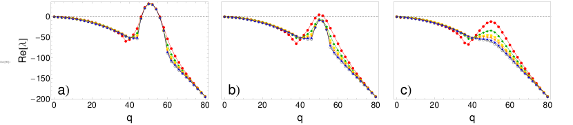
Figure 3: Largest branch of the real part of the growth rate given by solution of (7) for $\bar{\rho}=2000$, $\epsilon=0.0333$, $D_{r}=0.1$, $R=0.1$ and $D=3\times 10^{-2}$. The number of modes $M$ is 3 (red disks), 5 (green diamonds), 7 (yellow squares), 9 (orange triangles), 11 (blue stars) and 13 (black circles). a) $U_{0}=1.75$, b) $U_{0}=2.4$ and c) $U_{0}=3$.

We can now check the accuracy of truncating at different values of $M$. If enough modes $M$ have been included, the predictions obtained for higher values of $M$ should collapse on the same curve. It appears that the higher the self-propulsion, the higher $M$ needs to be to reach convergence: indeed, figure 3 shows that $M=3$ modes are enough for $U_{0}=1.75$, but we need at least $M=5$ modes for $U_{0}=2.4$. Note that for $U_{0}=3$, $M=13$ modes are barely enough. Therefore, keeping only a small number of modes will accurately describe the structural transition only if this one takes place for a small value of $U_{0}$, meaning that the system is already quite close to the critical point. However, we will see in the following subsection that they contain qualitatively the relevant mechanisms shaping the cluster crystals.

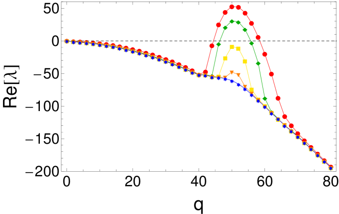
Figure 4: Largest branch of the real part of the growth rate $\lambda$ given by solution of (7). Same parameters as in figure 1 a) except $U_{0}=1$ (red disks), $1.75$ (green diamonds), $2.4$ (yellow squares), $2.7$ (orange triangles) and $3$ (blue stars). Continuous fraction defining $f(\lambda,q)$ truncated at $M=13$.

Figure 4 shows the maximum real part of the growth rate as a function of $q$ for several values of $U_{0}$. The continuous fraction defining $f(\lambda,q)$ has been truncated to $M=13$, which is sufficiently large for the results to remain unchanged when increasing $M$ further. In the passive case Delfau et al. (2016) and for the GEM-3 potential the homogeneous state becomes first unstable with respect to a wavenumber $q_{c}$ depending only on the interaction range $R$ and satisfying $q_{c}R\approx 5.0$. This corresponds to a cluster crystal of periodicity $2\pi/q_{c}\approx 1.26R$. For the parameters used here, for which $R=0.1$, we have $q_{c}\approx 50$. In Fig. 4 we see that a very similar wavenumber is the most unstable in the active case for small $U_{0}$. When $U_{0}$ is sufficiently increased though, these positive growth rates eventually become negative. Activity thus stabilizes the homogeneous state and prevents clustering, in agreement with our particle simulations.

More quantitatively, one can compare the values of the transition threshold $U_{0}^{c}$ obtained analytically for sufficiently large $M$, and from particle simulations. For the second case we start from an initial hexagonal crystal of clusters and increase $U_{0}$ step-by-step until we get a long-lived gas phase. Table 1 shows that the linear stability analysis gives us the right order of magnitude but it systematically underestimates the threshold. We attribute this to the nature of the transition, which in the passive-particle case is subcritical and subject to hysteresis Delfau et al. (2016). We expect this subcritical nature to remain also for small $U_{0}$. Also, the use of a deterministic version of the DK equation, as an approximation to the complete stochastic one, may be a source of error.

$10^{2}\times D$	3.0	4.0	5.0	5.4
$U_{0}^{c}$ (simulations)	2.65	2.05	1.45	1.35
$U_{0}^{c}$ (linear theory)	2.33	1.87	1.15	0.5

Table 1: Critical self-propulsion $U_{0}^{c}$ above which the cluster crystal disappears, obtained from particle simulations and from the linear stability analysis of (III.1). $\bar{\rho}=2000$, $D_{r}=0.1$ and a GEM-3 potential with $R=0.1$ and $\epsilon=0.0333$.

III.2 Macroscopic equation for 2 modes

Equations (2) or (III.1) are quite involved and it would be desirable to work with a simpler set of equations such as a small-$M$ truncation of (III.1). The linear analysis reveals that this is in general not an accurate approach, as values up to $M=13$ need to be considered to have convergence of the growth rates. This is so because, except for the largest values of $D_{r}$ or the smallest $U_{0}$, the average velocity field at each point has a well-defined direction (see for example figure 1 b) and many angular modes are needed to represent such localized distribution in $\theta$ space. Nevertheless a truncation to order $M=1$ leads to relatively simple equations which give insight into the physical mechanisms and favor qualitative understanding. Following Bertin et al. Bertin et al. (2009), we consider a hypothetical situation in which $\varepsilon=|\rho_{1}/\rho_{0}|<<1$ and then $\rho_{n}({\bf x},t)=\mathcal{O}(\varepsilon^{|n|})$, so that we can neglect the modes beyond $n=\pm 1$ (truncation to $M=1$). We get:

$$\partial_{t}\rho({\bf x},t) =-\nabla\cdot\left({\boldsymbol{F}}_{\rho}({\bf x},t)\rho({\bf x},t)\right)+D\nabla^{2}\rho({\bf x},t)-U_{0}\nabla\cdot{\boldsymbol{P}}({\bf x},t)$$

$$\partial_{t}{\boldsymbol{P}}({\bf x},t) =-\nabla\cdot\left({\boldsymbol{F}}_{\rho}({\bf x},t){\boldsymbol{P}}({\bf x},t)\right)+D\nabla^{2}{\boldsymbol{P}}({\bf x},t)-D_{r}{\boldsymbol{P}}({\bf x},t)$$ (10)

$$-\frac{U_{0}}{2}\nabla\rho({\bf x},t)\ ,$$

where ${\boldsymbol{P}}({\bf x},t)=\left(\begin{array}[]{c}\mbox{Re}\left[\rho_{1}\right]\\ \mbox{Im}\left[\rho_{1}\right]\end{array}\right)=\int\rho({\bf x},\theta,t){\bf\hat{n}}(\theta)d\theta$ is the momentum or polarization field. The product ${\boldsymbol{F}}_{\rho}{\boldsymbol{P}}$ appearing in (10) is a tensor product. Even if Eqs. (10) are a rough approximation to (III.1) they still describe the system behavior qualitatively. Integrating numerically Eqs. (10) with a spectral method using $512\times 512$ grid points, we recover the crystal of clusters for small values of $U_{0}$ (see figure 1 c) and a homogeneous state for higher $U_{0}$. The polarization structure of the clusters is also in good agreement with our previous observations: Fig. 1 d) shows that the polarization field inside the clusters is radial. Empty clusters are also observed in one dimension for small $D$ and high enough $U_{0}$. Having to work at small values of $D$ makes it more difficult to obtain empty clusters in two dimensions because of the need of a high numerical resolution. We have shown however than Eqs. (10) support clusters with a depletion in their center (see figure 2 b) if we replace the convolution product defining $\boldsymbol{F}_{\rho}$ by an effective confinement potential justified by the approximation described in the next paragraph.

Eqs. (10) serve also as a starting point to better understand the mechanisms shaping cluster structure. As in the passive case Delfau et al. (2016) we can focus on the case of small $D$ so that a first approximation for the steady crystal density is a set of delta functions at the lattice points $\{{\bf a}_{i}\}$: $\rho({\bf x})\approx N_{p}\sum_{\{{\bf a}_{i}\}}\delta({\bf x}-{\bf a}_{i})$. The number of particles per cluster, $N_{p}$, can be expressed in terms of $\bar{\rho}$ and the intercluster distance $a$: $N_{p}=\bar{\rho}a^{2}\sqrt{3}/2$. With this approximation ${\boldsymbol{F}}_{\rho}({\bf x})\approx-N_{p}\sum_{\{{\bf a}_{i}\}}\nabla V({\bf x}-{\bf a}_{i})$. To consider the structure of a narrow cluster centered at ${\bf x}={\bf 0}$ we keep in the lattice sum only the central and the six neighboring clusters, and expand around ${\bf x}\approx{\bf 0}$. For a GEM-$\alpha$ potential with $\alpha<2$ the dominant term is the interparticle repulsion within the central cluster, so that ${\boldsymbol{F}}_{\rho}({\bf x})$ points outwards and, as it is observed, the aggregate disappears. But when $\alpha>2$ the repulsion from the neighboring clusters prevails and produces a confining effective force at ${\bf x}\approx{\bf 0}$ overcoming the local repulsion. At first order in the distance ${\bf x}$ to the cluster center, we have ${\boldsymbol{F}}_{\rho}({\bf x})\approx-\gamma~{}{\bf x}$. $\gamma$ depends on $N_{p}$, on the intercluster distance $a$ and on the interaction potential parameters $\epsilon$ and $\rho$. Its precise expression is not particularly illuminating, but it can be found as $\gamma=D/\sigma_{2D}^{2}$ with $\sigma_{2D}$ given by Eq. (33) in Delfau et al. (2016). The harmonic character and radial symmetry of this approximation reduces the problem in Eqs. (10) to a stationary linear one for $\rho({\bf x})=\rho(r)$ and ${\boldsymbol{P}}({\bf x})=p_{r}(r){\bf\hat{e}_{r}}$ in polar coordinates centered at the cluster center (${\bf\hat{e}_{r}}$ is the unit vector in the radial direction) in the confining harmonic force $-\gamma r$ arising from the repulsion by neighboring clusters:

$$D\rho^{\prime}+\gamma r\rho-U_{0}p_{r}=0$$ (11)

$$Dp_{r}^{\prime\prime}+(\gamma r+\frac{D}{r})p_{r}^{\prime}+(2\gamma-D_{r}-\frac{D}{r^{2}})p_{r}-\frac{U_{0}}{2}\rho^{\prime}=0\ .$$

To get the equation for $\rho$, a first integral has already been performed under the condition of zero net particle flux in or out of the cluster, as appropriate for the steady state. The system (11) should be solved in $r\in[0,\infty]$, but the approximations used are valid only if it gives a cluster width much smaller than the interaction range $R$. The first equation in (11) shows that in the limit of small $U_{0}$, this cluster width is of the order of $w\approx\sqrt{D/\gamma}$. Eqs. (11) require three initial or boundary conditions, which could be taken as the values of $\rho$, $p_{r}$ and $p_{r}^{\prime}$ at $r=0$. Regularity of the field ${\boldsymbol{P}}({\bf x})$ at the origin implies $p_{r}(0)=0$ — which was observed for chemorepulsive active colloids Liebchen et al. (2015)— and $p_{r}(r\approx 0)\approx\nu r$ (so that $\nu=p_{r}^{\prime}(0)$). $\rho(0)$ can be determined by fixing the number of particles in the cluster $\int_{0}^{\infty}2\pi rdr\rho(r)=N_{p}$. In terms of it and of $p_{r}(r)$ the first equation in (11) can be solved explicitly:

$$\rho(r)=\left[\rho(0)+\frac{U_{0}}{D}\int_{0}^{r}e^{\frac{\gamma u^{2}}{2D}}p_{r}(u)du\right]e^{-\frac{\gamma r^{2}}{2D}},$$ (12)

which shows that there is a shape change, in agreement with the particle simulations, from a maximum of density at the origin ($\rho^{\prime\prime}(0)<0$) to a minimum ($\rho^{\prime\prime}(0)>0$) when the polarization slope at the origin $\nu=p_{r}^{\prime}(0)$ changes from $\nu U_{0}<\gamma\rho(0)$ to $\nu U_{0}>\gamma\rho(0)$, respectively. Finally, the condition $|{\boldsymbol{P}}({\bf x})|\leq\rho({\bf x})$ — resulting from the definition of ${\boldsymbol{P}}$ — imposes the value of this slope: $\nu$ must indeed cancel the prefactor of the slow decay at large $r$, $p_{r}\sim r^{-\mu}$ with $\mu=2-(D_{r}/\gamma)-U_{0}^{2}/(2D\gamma)$, arising from the large-$r$ behavior of the hypergeometric function that solves the homogeneous part of the (11) for $p_{r}(r)$. This determination can only be done numerically.

Figure 5: Particle density $\rho(r)$ and radial component of the polarization $p_{r}(r)$ from Eqs. (11). He have taken $\rho(0)=1$ and a dimensionless formulation in which the parameters are $\tilde{D}_{r}=D_{r}/\gamma=10^{-6}$ and $\tilde{U}_{0}=U_{0}/\sqrt{\gamma D}$. a) $\tilde{U}_{0}=0.8$. b) $\tilde{U}_{0}=1.4$.

Figure 5 shows examples of solutions of the radial equations (11), displaying the two qualitatively different cluster shapes, with smaller/larger density at the center. Although the truncation to $M=1$ leading to Eqs. (10) and (11) precludes quantitative agreement with particle simulations, Fig. 5 (see also figure 2 b) shows that this 2-mode truncation contains the essential qualitative mechanisms needed for the cluster-crystal formation and the structure of the clusters: an effective potential which confines particles within clusters, originating from the repulsion by the neighboring clusters, and the presence of a polarization field ${\boldsymbol{P}}$, increasing with $U_{0}$, which pushes the particles towards the periphery of the clusters until destroying them.

IV Conclusion

We have shown that ACCs occur in systems of active Brownian particles with soft repulsive interactions. Self-propulsion deforms the clusters by depleting particle density inside, and large self-propulsion stabilizes the homogenous-isotropic state. We have derived a continuous description and analyzed the crystal forming instability by linear analysis. Truncation to two angular modes, despite not being quantitatively accurate, retains the basic mechanisms. In particular it allows to understand crystal persistence as an effect of the confining forces arising from repulsion by neighboring clusters, and the cluster shape as a balance between the confining force and the tendency to radial escape driven by the polarization field.

We acknowledge financial support from grants LAOP, CTM2015-66407-P (AEI/FEDER, EU) and ESOTECOS, FIS2015-63628-C2-1-R (AEI/FEDER, EU).

References

References

- Ramaswamy (2010) S. Ramaswamy, Annual Review of Condensed Matter Physics 1, 323 (2010).
- Cates et al. (2010) M. E. Cates, D. Marenduzzo, I. Pagonabarraga, and J. Tailleur, Proceedings of the National Academy of Sciences of the United States of America 107, 11715 (2010).
- Marchetti et al. (2013) M. C. Marchetti, J. F. Joanny, S. Ramaswamy, T. B. Liverpool, J. Prost, M. Rao, and R. A. Simha, Reviews of Modern Physics 85, 1143 (2013).
- Romanczuk et al. (2012) P. Romanczuk, M. Bär, W. Ebeling, B. Lindner, and L. Schimansky-Geier, The European Physical Journal Special Topics 202, 1 (2012).
- Mani and Löwen (2015) E. Mani and H. Löwen, Physical Review E 92, 032301 (2015).
- Menzel et al. (2014) A. M. Menzel, T. Ohta, and H. Löwen, Physical Review E 89, 022301 (2014).
- Menzel and Löwen (2013) A. M. Menzel and H. Löwen, Phys. Rev. Lett. 110, 055702 (2013).
- Cates and Tailleur (2015) M. E. Cates and J. Tailleur, Annual Review of Condensed Matter Physics 6, 219 (2015).
- Mognetti et al. (2013) B. M. Mognetti, A. Sarić, S. Angioletti-Uberti, A. Cacciuto, C. Valeriani, and D. Frenkel, Physical Review Letters 111, 245702 (2013).
- Redner et al. (2013) G. S. Redner, A. Baskaran, and M. F. Hagan, Physical Review E 88, 012305 (2013).
- Tailleur and Cates (2008) J. Tailleur and M. E. Cates, Physical Review Letters 100, 218103 (2008).
- Fily and Marchetti (2012) Y. Fily and M. C. Marchetti, Physical Review Letters 108, 235702 (2012).
- Farrell et al. (2012) F. D. C. Farrell, M. C. Marchetti, D. Marenduzzo, and J. Tailleur, Physical Review Letters 108, 248101 (2012).
- Cates and Tailleur (2013) M. E. Cates and J. Tailleur, EPL (Europhysics Letters) 101, 20010 (2013).
- Stenhammar et al. (2013) J. Stenhammar, A. Tiribocchi, R. J. Allen, D. Marenduzzo, and M. E. Cates, Physical Review Letters 111, 145702 (2013).
- Bialké et al. (2013) J. Bialké, H. Löwen, and T. Speck, EPL (Europhysics Letters) 103, 30008 (2013).
- Fily et al. (2014) Y. Fily, S. Henkes, and M. C. Marchetti, Soft Matter 10, 2132 (2014).
- Buttinoni et al. (2013) I. Buttinoni, J. Bialké, F. Kümmel, H. Löwen, C. Bechinger, and T. Speck, Phys. Rev. Lett. 110, 238301 (2013).
- Theurkauff et al. (2012) I. Theurkauff, C. Cottin-Bizonne, J. Palacci, C. Ybert, and L. Bocquet, Phys. Rev. Lett. 108, 268303 (2012).
- Klein et al. (1994) W. Klein, H. Gould, R. A. Ramos, I. Clejan, and A. I. Mel’cuk, Physica A: Statistical Mechanics and its Applications 205, 738 (1994).
- Likos et al. (2001) C. N. Likos, A. Lang, M. Watzlawek, and H. Löwen, Physical Review E 63, 031206 (2001).
- Mladek et al. (2006) B. M. Mladek, D. Gottwald, G. Kahl, M. Neumann, and C. N. Likos, Physical Review Letters 96, 045701 (2006).
- Likos et al. (2007) C. Likos, B. M. Mladek, D. Gottwald, and G. Kahl, The Journal of Chemical Physics 126, 224502 (2007).
- Mladek et al. (2008) B. M. Mladek, G. Kahl, and C. N. Likos, Physical Review Letters 100, 028301 (2008).
- Coslovich and Ikeda (2013) D. Coslovich and A. Ikeda, Soft Matter 9, 6786 (2013).
- Menzel and Ohta (2012) A. M. Menzel and T. Ohta, EPL (Europhysics Letters) 99, 58001 (2012).
- Menzel (2013) A. M. Menzel, Journal of Physics: Condensed Matter 25, 505103 (2013).
- Delfau et al. (2016) J.-B. Delfau, H. Ollivier, C. López, B. Blasius, and E. Hernández-García, Physical Review E 94, 042120 (2016).
- Toral and Colet (2014) R. Toral and P. Colet, Stochastic Numerical Methods: An Introduction for Scientists (Wiley-VCH, 2014).
- Nash et al. (2010) R. W. Nash, R. Adhikari, J. Tailleur, and M. E. Cates, Phys. Rev. Lett. 104, 258101 (2010).
- Menzel (2015) A. M. Menzel, EPL (Europhysics Letters) 110, 38005 (2015), ISSN 0295-5075.
- Menzel et al. (2016) A. M. Menzel, A. Saha, C. Hoell, and H. Löwen, The Journal of Chemical Physics 144, 024115 (2016).
- Kawasaki (1994) K. Kawasaki, Physica A: Statistical Mechanics and its Applications 208, 35 (1994).
- Dean (1996) D. S. Dean, Journal of Physics A: Mathematical and General 29, L613 (1996).
- Oksendal (2000) B. Oksendal, Stochastic Differential Equations (Springer, 2000).
- Speck et al. (2015) T. Speck, A. M. Menzel, J. Bialké, and H. Löwen, The Journal of Chemical Physics 142, 224109 (2015).
- Loi et al. (2008) D. Loi, S. Mossa, and L. F. Cugliandolo, Physical Review E 77, 051111 (2008).
- Palacci et al. (2010) J. Palacci, C. Cottin-Bizonne, C. Ybert, and L. Bocquet, Physical Review Letters 105, 088304 (2010).
- Bertin et al. (2009) E. Bertin, M. Droz, and G. Grégoire, Journal of Physics A: Mathematical and Theoretical 42, 445001 (2009).
- Liebchen et al. (2015) B. Liebchen, D. Marenduzzo, I. Pagonabarraga, and M. E. Cates, Physical Review Letters 115, 258301 (2015).