Recent advances in liquid mixtures in electric fields

Abstract

When immiscible liquids are subject to electric fields interfacial forces arise due to a difference in the permittivity or the conductance of the liquids, and these forces lead to shape change in droplets or to interfacial instabilities. In this Topical Review we discuss recent advances in the theory and experiments of liquids in electric fields with an emphasis on liquids which are initially miscible and demix under the influence of an external field. In purely dielectric liquids demixing occurs if the electrode geometry leads to sufficiently large field gradients. In polar liquids field gradients are prevalent due to screening by dissociated ions irrespective of the electrode geometry. We examine the conditions for these “electro prewetting” transitions and highlight few possible systems where they might be important, such as in stabilization of colloids and in gating of pores in membranes.

I Introduction

Electrostatic forces are ubiquitous and their effect is important in many soft matter systems involving liquids bounded by hard or soft walls. They arise on purpose and are easily controlled when water or other solvents flow in microfluidics channels in contact with a metallic electrode whose potential is externally controlled. They are less easily controlled when the solvent is nearby a charged nonmetallic surface which can induce or impede the flow. In biological settings electrostatic forces determine whether proteins or other molecules bind to other molecules or to cellular structure which are often charged. When colloids are suspended in solvents the competition between entropic and electrostatic forces may lead to inter-colloidal attraction and eventually to coagulation and sedimentation of the colloids, or to repulsion between the colloids and to stabilization of the suspension. The interplay between shear forces, surface tension and electrostatic also plays a vital role in many industrial process where liquid droplets are transported and ejected via small orifices, as occurs for example in pesticide spraying in agriculture or in ink-jet printing.

This paper gives a concise overview of interfacial instabilities that occur when electric fields are applied in a direction perpendicular to an initially flat interface between two liquids. Sec. II.1 discusses this normal-field instability in purely dielectric liquids where the electrostatic forces destabilizing the interface are proportional to the difference between the liquids’ permittivities squared. The situation is more complex when residual conductivity exists in the liquid phases and in this case mobile dissociated ions exert shear forces on the interface and modify its shape, Sec. II.2.

Section III then poses a more fundamental question: what if electric fields could affect the relative miscibility of the two liquids? Namely, not only alter the interface but destroy it? Sec. III.1 shows the Landau theory that addressed this question and proved that indeed such possibility exists. The experiments supporting and contradicting the Landau theory are summarized in Sec. III.2.

Section IV goes one step further and examines situations where electric field gradients act on dielectric liquids. In these systems a dielectrophoretic force acts on the liquids and, if strong enough, it may lead to demixing of the liquids from each other. In those cases the shape, size and location of the electrodes producing the fields are crucial for the understanding of the statics and dynamics of the phase transitions. Peculiarly, an interfacial instability exists where the electric field stabilizes the interface while surface tension destabilizes it, in contrast to the normal-field instability of Secs. II.1 and II.2. New experimental results of phase separation dynamics and equilibrium are shown and analyzed.

Demixing occurs also in mixtures of polar solvents, but this time due to screening of the field which always exist irrespective of the electrodes. The “electro-prewetting” transitions described in Sec. V have a specific dependence on the salt content, temperature and relative composition of the mixture. The relative miscibility of the ions in the solvents plays a crucial role.

After surveying the basic physical concepts two “applications” are considered: Sec. VI gives an account of the electrostatic and van der Waals forces between two colloids immersed in a polar solution. The section details the complex interplay between these forces that depends on the relative adsorption of the liquids at the surface of the colloids, in addition to the temperature and mixture composition. Contrary to the regular Derjaguin, Landau, Verwey, and Overbeek (DLVO) behavior in simple liquids here the addition of ions leads to a repulsion between the colloids in a certain window of parameters. Sec. VII considers another situation where polar liquids are found in contact with hard surfaces: porous membranes. Pore gating between two states can be achieved by controlling the surface potential of the membrane. This gating of membranes to small molecules by external potentials could be advantageous over other methods. Finally Sec. VIII is a summary and outlook.

II Force and stress in liquids in electric fields

When a liquid is placed under the influence of an electric field ${\bf E}$ stress develops. This stress originates from the electrostatic free energy density $-(1/2){\bf E}\cdot{\bf D}$, where ${\bf D}=\varepsilon{\bf E}$ is the displacement field and $\varepsilon$ is the local dielectric constant. Due to the vectorial nature of the field, the stress $\overleftrightarrow{T}$ is tensorial. For a unit surface whose normal is $\hat{n}$, the force acting on that surface is given by $-\overleftrightarrow{T}\cdot\hat{n}$ (the i’th component is $-\overleftrightarrow{T}_{\rm ij}n_{j}$ where we have used the summation convention on the index $j$). The electric field has diagonal and non-diagonal contributions to the stress tensor Landau and Lifshitz (1957); Melcher (1963); Saville (1997)

$$\overleftrightarrow{T}_{\rm ij}=-p_{0}(c,T)\delta_{\rm ij}+\frac{1}{2}\varepsilon E^{2}\left(-1+\frac{c}{\varepsilon}\left(\frac{\partial\varepsilon}{\partial c}\right)_{T}\right)\delta_{\rm ij}+\varepsilon E_{i}E_{j}$$ (1)

Here $p_{0}(c,T)$ is the equation of state of the liquid in the absence of field, where $c$ is the density and $T$ is the temperature. In fluids the “regular” pressure has a diagonal contribution to $\overleftrightarrow{T}_{\rm ij}$.

The body force ${\bf f}$ is given as a divergence of the this stress: $f_{i}=\partial\overleftrightarrow{T}_{\rm ij}/\partial x_{j}$, and is given by

$${\bf f}=-\nabla p_{0}+\frac{1}{2}\nabla\left(E^{2}c\frac{\partial\varepsilon}{\partial c}\right)_{T}-\frac{1}{2}E^{2}\nabla\varepsilon+\rho{\bf E}$$ (2)

where $\rho$ is the charge density. The second and third terms describe electrostriction and dielectrophoretic forces whereas the last term reflects the force that is transferred to the liquid by free moving charges.

The discontinuity of the normal field across the interface is obtained as

$$\llbracket{\bf D}\rrbracket\cdot\hat{n}=\sigma$$ (3)

where $\llbracket{\bf D}\rrbracket\equiv{\bf D}^{(2)}-{\bf D}^{(1)}$ is the discontinuity of the displacement field across the interface, $\sigma$ is the surface charge density, and the surface unit vector $\hat{n}$ points from region 1 to region 2. The continuity of the tangential field across the interface is given by

$$\llbracket{\bf E}\rrbracket\cdot\hat{t_{i}}=0$$ (4)

where $\hat{t}_{i}$ ($i=1$, $2$) are the two orthogonal unit vector lying in the plane of the interface. At the interface between two regions of different permittivity the force is discontinuous. The i’th component of the net force per unit area of the interface, ${\bf f}_{s}$, is given by

$${\bf f}_{{\rm s,}i}=\llbracket\overleftrightarrow{T}_{\rm ij}\rrbracket n_{j}$$ (5)

where $\llbracket\overleftrightarrow{T}_{\rm ij}\rrbracket=\overleftrightarrow{T}_{\rm ij}^{(2)}-\overleftrightarrow{T}_{\rm ij}^{(1)}$. When the isotropic parts of the force can be neglected [first and second terms in Eq. (2)], the electric field bisects the angel between $\hat{n}$ and the direction of the resultant force acting on the surface. This can be seen by choosing the x-axis to be parallel to ${\bf E}$ and by noting that $\hat{\bf f}_{\rm s}\cdot\hat{\bf E}$ equals $\hat{\bf f}_{\rm s}\cdot\hat{n}$ K. H. Panofsky and Phillips (2005).

The net force per unit area has three components: one in the direction perpendicular to the surface (parallel to $\hat{n}$) and two in directions parallel to $\hat{t}_{i}$. They are Saville (1997)

$$\llbracket\overleftrightarrow{T}\cdot\hat{n}\rrbracket\cdot\hat{n} = \frac{1}{2}\llbracket\left({\bf E}\cdot\hat{n}\right)^{2}-\left({\bf E}\cdot\hat{t}_{1}\right)^{2}-\left({\bf E}\cdot\hat{t}_{2}\right)^{2}-p_{0}+c\frac{\partial\varepsilon}{\partial c}E^{2}\rrbracket$$

$$\llbracket\overleftrightarrow{T}\cdot\hat{n}\rrbracket\cdot\hat{t}_{i} = \sigma{\bf E}\cdot\hat{t}_{i}~{},~{}~{}~{}i=1,2$$ (6)

In the second equation we used Eqs. (3) and (4).

A body force induces flow in the liquid. The Navier-Stokes equation for the the flow velocity ${\bf u}$ in incompressible liquids is

$$c\left[\frac{\partial{\bf u}}{\partial t}+\left({\bf u}\cdot\nabla\right){\bf u}\right]=-\nabla p_{0}+\frac{1}{2}\nabla\left(E^{2}c\frac{\partial\varepsilon}{\partial c}\right)_{T}-\frac{1}{2}E^{2}\nabla\varepsilon+\rho{\bf E}+\eta\nabla^{2}{\bf u}.$$ (7)

Here $\eta$ is the fluid’s viscosity and the $i$th component of $\nabla^{2}{\bf u}$ is $\nabla^{2}u_{i}$. The term $\left({\bf u}\cdot\nabla\right){\bf u}$ is a vector whose $i$th component is ${\bf u}\cdot\nabla u_{i}$.

II.1 Normal field instability in two immiscible dielectric liquids

Let us illustrate the force and stress in a simple example – a bilayer of two purely dielectric liquids, 1 and 2, with dielectric constants $\varepsilon_{1}$ and $\varepsilon_{2}$, respectively, sandwiched inside a parallel-plate capacitor, see Fig. 1a. The distance between the plates is $L$ and the thickness of the first liquid is $h$. In this geometry the electric fields ${\bf E}_{1}$ and ${\bf E}_{2}$ are oriented in the $z$-direction and are constant within the two regions. They are found from the boundary conditions on the interface $\varepsilon_{1}E_{1}=\varepsilon_{2}E_{2}$ (Eq. (3) with $\sigma=0$) and from $E_{1}h+E_{2}(L-h)=E_{0}L$, where $E_{0}$ is the average electric field imposed by the capacitor. One thus finds that

$${\bf E}_{1} = \frac{\varepsilon_{2}E_{0}}{\varepsilon_{1}(1-h/L)+\varepsilon_{2}h/L}\hat{z}~{},~{}~{}~{}~{}~{}~{}{\bf E}_{2}=\frac{\varepsilon_{1}E_{0}}{\varepsilon_{1}(1-h/L)+\varepsilon_{2}h/L}\hat{z}~{}.$$ (8)

From Eq. (1), when $\partial\varepsilon/\partial c=0$ the stresses just “below” and just “above” the interface, $\overleftrightarrow{T}_{\rm zz}^{(1)}$ and $\overleftrightarrow{T}_{\rm zz}^{(2)}$, respectively, are then given by

$$\overleftrightarrow{T}_{\rm zz}^{(1)}=\frac{1}{2}\frac{\varepsilon_{1}\varepsilon_{2}^{2}E_{0}^{2}}{\left(\varepsilon_{1}(1-h/L)+\varepsilon_{2}h/L\right)^{2}}~{},~{}~{}~{}~{}~{}~{}~{}\overleftrightarrow{T}_{\rm zz}^{(2)}=\frac{1}{2}\frac{\varepsilon_{2}\varepsilon_{1}^{2}E_{0}^{2}}{\left(\varepsilon_{1}(1-h/L)+\varepsilon_{2}h/L\right)^{2}}$$ (9)

Since these stresses are constant throughout the bulk of the liquids there is no body force of electrostatic origin. The difference

$$\overleftrightarrow{T}_{\rm zz}^{(2)}-\overleftrightarrow{T}_{\rm zz}^{(1)}=-\frac{1}{2}\frac{\varepsilon_{1}\varepsilon_{2}\Delta\varepsilon E_{0}^{2}}{\left(\varepsilon_{1}+\Delta\varepsilon h/L\right)^{2}}$$ (10)

gives the net stress on the interface. Here we used $\Delta\varepsilon\equiv\varepsilon_{2}-\varepsilon_{1}$. If $\Delta\varepsilon$ is positive the interface is pushed downwards so as to decrease $h$, if $\Delta\varepsilon$ is negative then the interface is pushed upwards.

Under sufficiently large electric field an interfacial instability may occur and this can be seen as follows. Assume the bilayer divides into two parts, one with small value of $h$ and one with a large value, as is depicted in Fig. 1b. In this idealized picture all three interfaces, marked by ‘a’, ‘b’, ‘c’, are either parallel or perpendicular to the electrodes. Far from interface ‘b’ the fringe field can be ignored and the field is still in the $z$-direction. In each domain the expressions for the fields stay the same as in Eq. (8).

As Eq. (10) shows the stress is largest when $h$ is smallest; for incompressible liquids this means that if the interface ‘a’ pushes downwards interface ‘c’ will “cede” and will move upwards to conserve the volume of liquid 1. The conclusion is that the interface illustrated in Fig. 1b is not stable; in the long time the film will be divided to two liquid domains 1 and 2 with an interface perpendicular to the electrodes (and parallel to the field). In this equilibrium state the fields in both liquids are equal: ${\bf E}_{1}={\bf E}_{2}=E_{0}\hat{z}$. The stress tensor $\overleftrightarrow{T}_{\rm ij}$ from Eq. (1) is then diagonal and continuous across the interface, hence no net surface force acts to displace the interface.

At early times the destabilization of an initially flat interface is characterized by a fastest growing $q$-mode modulation of the surface. Let $h(x,t)$ be the thickness of the layer of the first liquid and for simplicity assume the second liquid is gas. For thin films a Poiseuille flow is assumed where the $x$-component of the flow velocity vanishes at $z=0$ and is maximal at $z=h$. The integration of ${\bf u}$ in Eq. (7) along the $z$ coordinate gives a flux

$$-\frac{h^{3}}{3\eta}\frac{\partial p}{\partial x}$$ (11)

The pressure has three contributions Herminghaus (1999): one is the disjoining pressure given by $A/6h^{3}$ due to van der Waals forces, where $A$ is the effective Hamaker constant of the system, the second occurs in curved interfaces where surface tension plays a role: $-\gamma h^{\prime\prime}(x)$, where $\gamma$ is the surface tension between the two layers. The third contribution to the pressure is electrostatic.

At the initial destabilization state the interface is only weakly perturbed and $h(x)$ can be written as $h(x)=h_{0}+\delta h(x,t)$, where $h_{0}$ is the average film thickness and $\delta h\ll h_{0}$ is the small spatially-dependent perturbation growing in time. In the long wavelength approximation $\delta h^{\prime}\ll 1$ and to lowest (linear) order in $\delta h$ one can write the pressure as

$$p(x)=-\frac{A}{2h_{0}^{4}}\delta h-\gamma\delta h^{\prime\prime}-\frac{\varepsilon_{1}\varepsilon_{2}\left(\Delta\varepsilon\right)^{2}E_{0}^{2}}{L\left(\varepsilon_{1}+\Delta\varepsilon h_{0}/L\right)^{3}}\delta h+{\rm const.}$$ (12)

The set of equations for $\delta h$ is complete when one uses Eq. (12) and Eq. (11) together with the “continuity” equation for $h$: $\partial h/\partial t+\partial\left(-h^{3}/(3\eta)\partial p/\partial x\right)/\partial x=0$. In this linear approximation one may substitute a sinusoidal ansatz with q-number $q$ and growth rate $\omega$: $\delta h=e^{iqx+\omega t}$ to obtain the dispersion relation between $\omega$ and $q$:

$$\omega(q)=\frac{\gamma h_{0}^{3}}{3\eta}\left(\xi_{e}^{-2}q^{2}-q^{4}\right)$$ (13)

where

$$\xi_{e}^{-2}=\frac{A}{2\gamma h_{0}^{4}}+\frac{\varepsilon_{1}\varepsilon_{2}\left(\Delta\varepsilon\right)^{2}E_{0}^{2}}{\gamma L\left(\varepsilon_{1}+\Delta\varepsilon h_{0}/L\right)^{3}}$$ (14)

is the healing length having two contributions, from van der Waals and from electrostatics, both weighed against surface tension Herminghaus (1999); Pease and Russel (2002).

In Eq. (13) the dependence of $\omega$ on $q$ has a positive contribution scaling as $q^{2}$ and a negative contribution proportional to $-q^{4}$ and thus for small $q$ values $\omega(q)$ is positive and increases with increasing $q$. The growth rate $\omega(q)$ for all $q$’s smaller than $\xi_{e}^{-1}$ is positive and they are unstable; modulations with large enough $q$’s, $q>\xi_{e}^{-1}$, are stable and diminish exponentially with time. The fastest growing $q$-mode obeys $\partial\omega(q)/\partial q=0$ and hence

$$q_{\rm fastest}=\frac{1}{\sqrt{2}}\xi_{e}^{-1}~{},~{}~{}~{}~{}~{}~{}\omega_{\rm fastest}=\frac{\gamma h_{0}^{3}}{12\eta}\xi_{e}^{-4}~{}.$$ (15)

Which of the two forces is more dominant, the dispersion or electrostatic force? The van der Waals pressure scales as $A/h_{0}^{3}$ whereas the electrostatic pressure is $\sim\varepsilon E_{0}^{2}$. If we take the field to be $E_{0}\simeq 1$V/$\mu$m, $\varepsilon\simeq\varepsilon_{0}$ ($\varepsilon_{0}$ is the vacuum permittivity), and $A\simeq 10^{-20}$J we find that for film thicknesses $h_{0}$ larger than $\sim 10$nm the electrostatic force is the dominant force. For such relatively thick films the pattern period $2\pi/q_{\rm fastest}$ observed in experiments scales as $\gamma^{1/2}/(\Delta\varepsilon E_{0})$ and can be thus reduced if the surface tension is decreased or if the “dielectric contrast” $\Delta\varepsilon$ or electric fields are increased Schaffer et al. (2000); Lau and Russel (2011); Lin et al. (2001, 2002); Wu et al. (2006); Goldberg-Oppenheimer and Steiner (2010).

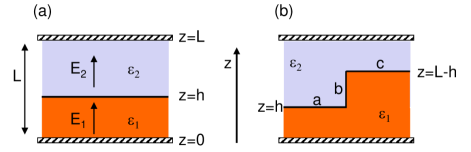
Figure 1: Two liquids in electric field. (a) Schematic illustration of a bilayer of two liquids 1 and 2 with permittivities $\varepsilon_{1}$ and $\varepsilon_{2}$, respectively, confined by a parallel-plates capacitor whose plates are at $z=0$ and $z=L$. The thickness of the liquid layers are $h$ and $L-h$. The fields ${\bf E}_{1}$ and ${\bf E}_{2}$ are oriented in the $z$-direction. (b) Idealized configuration where the bilayer breaks into two parts, with small (left side) and large (right side) values of $h$. ‘a’, ‘b’, and ‘c’ mark the three interfaces.

II.2 The role of a small residual conductivity

In the classical experiments with liquid droplets embedded in an immiscible liquid under the influence of an external field the droplets elongated in the direction of the field, as expected O’Konski and Thacher (1953); Allan and Mason (1962). In some cases, however, droplets became oblate rather than prolate. Taylor and Melcher realized the importance of shear stress due to a small number of dissolved ions Taylor (1966); Melcher and Taylor (1969). In perfectly conducting liquids the electric fields are always perpendicular to the interfaces and hence no shear force exists. In the other extreme, that of perfect dielectrics ($\sigma=0$), the force density is perpendicular to the surface and the shear component vanishes as well, as can be seen from the component of the force parallel to the interface, Eq. (II).

In Taylor’s “leaky dielectric” model the Maxwell shear stress of the residual charge must be balanced by a stress due to liquid flow inside and outside of the droplet. For a field alternating with angular frequency $\omega$ much larger than the typical inverse ion relaxation time $\Sigma/\varepsilon$, where $\Sigma$ is the electrical conductivity, the behavior of the liquid is similar to that of a pure dielectric since the ions move very little about their place. When the frequency is reduced below this threshold, $\omega<\Sigma/\varepsilon$, ions oscillation are large and they move about more significantly as the frequency is further reduced. In the limit of a DC field ($\omega\to 0$) clearly even a vanishingly small amount of ions can lead to a very strong response, recalling that $\Sigma$ is proportional to the ion number density.

Taylor analyzed the electrohydrodynamics problem and his derivation lead to a function $\Phi$ given by

$$\Phi=R\left(D^{2}+1\right)-2+3\left(RD-1\right)\frac{2M+3}{5M+5}$$ (16)

The parameters appearing $M$, $R$, and $D$ are the ratios of the values of viscosity, resistivity, and dielectric constant of the outer medium to that of the drop, respectively. Prolate drops are predicted when $\Phi>0$ while oblate drops correspond to $\Phi<0$. Spherical drops, $\Phi=0$, thus occur as a special case.

Based on this understanding one may ask how does residual conductivity affect the normal field instability described above? Namely how do the dispersion relation Eq. (13) and the fastest-growing $q$-mode Eq. (15) change when conductivity is taken into account? It turns out that the existence of ions leaves the general shape of the curve $\omega(q)$ intact but the maximum shifts to larger values – both the fastest-growing $q$-mode and its growth rate are increased Pease and Russel (2002).

Patterning of films using the normal-field instability is an appealing concept for nanotechnological applications because of its simplicity and small number of processing steps Schaffer et al. (2001, 2000); Morariu et al. (2003). A typical setup involves a polymer film of thickness $\approx 50$-$700$nm placed on a substrate, and a gap with varying thickness between the polymer and the mask. The idea is to quench the polymer structure at a specific time, at the onset of the instability, where the most unstable mode is dominant, or at a later time, where nonlinear structures with additional periodicities develop. Ideally one could increase the voltage and field across the substrate and mask to decrease the period of unstable mode indefinitely. However, when the electric field increases above $\sim 100$V/$\mu$m (depending on the polymer used and the overall sample geometry) dielectric breakdown marked by a spark occurs, and current flows between the two electrodes. A possible route to decrease the length-scale associated with the unstable mode, $\lambda\sim q_{\rm fastest}^{-1}$, is to decrease the surface tension $\gamma$, since $\lambda\sim\gamma^{1/2}$ when van der Waals forces can be neglected. A smart strategy is to fill the air gap between the polymer film and the mask with a second polymer, thereby creating a bilayer polymer system. The surface tension between the two polymers was indeed reduced this way but the dielectric contrast $\Delta\varepsilon$ was reduced too, and this had a detrimental effect. In addition, the leaky dielectric model has prompted researchers to use polymers with a small conductivity or even to replace one of the polymers by an ionic liquid Lau and Russel (2011). A comparison between the theoretical and experimental values of the fastest growing wavelength is shown in Fig. 2. This has led to a decrease in the feature size, though only down to a limit set by the dielectric breakdown of the thin polymer layer.

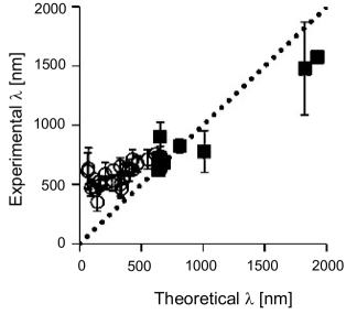
Figure 2: Experimental vs theoretical fastest growing wavelength in various experiments with varying film thicknesses and voltages. The liquids used were polystyrene and an ionic liquid. The average field is smaller than $139$V/$\mu$m (filled squares) and larger than $158$V/$\mu$m (open circles). The dotted line is the expected $\lambda_{\rm th}=\lambda_{\rm exp}$ relation. The deviation from this line occurs for high field strengths. Clearly the size reduction stops at $\simeq 400$nm. Adapted from Ref. Lau and Russel (2011).

III Changes in the relative miscibility of dielectric liquids

The preceding section described the interfacial instability that occurs when the stress by the electric field opposes the stress by the surface tension between two existing phases. But a more fundamental question arises: can the external field create or destroy an interface between two phases? That is, what is the effect of an electric field on the liquid-vapor coexistence of a pure component or the liquid-liquid coexistence for binary mixtures, and how is the critical point changed? A treatise on this problem was given by Landau.

III.1 Landau theory of critical effects of external fields on partially miscible dielectric liquids

In the book of Landau and Lifshitz Landau and Lifshitz (1957) the effect of a uniform electric field on the critical point was given as a short solved problem. Unfortunately it appeared only in the first edition of the book and was removed from the second edition by the Editors presumably because it was considered as “unimportant”. This unimportant problem has caught considerable attention in recent years.

We illustrate Landau’s reasoning for a binary mixture of two liquids, A and B. The phase diagram is given by $T$ and $\phi$, the volume fraction of A component ($0\leq\phi\leq 1$). The mixture’s free energy density $f_{\rm m}(\phi,T)$ includes the enthalpic contributions, favoring separation, and the entropic force, favoring mixing. The electrostatic energy density is $f_{\rm es}=-(1/2)\varepsilon(\phi)E^{2}$, where $\varepsilon(\phi)$ is a constitutive equation relating the local permittivity with the local composition. Close enough to the critical point $(\phi_{c},T_{c})$ one can expand the free energies in a Taylor series in the small deviation $\varphi\equiv\phi-\phi_{c}$

$$f_{\rm m} \simeq f_{\rm m}(\phi_{c},T)+\frac{\partial f_{\rm m}(\phi_{c},T)}{\partial\phi}\varphi+\frac{1}{2}\frac{\partial^{2}f_{\rm m}(\phi_{c},T)}{\partial\phi^{2}}\varphi^{2}+~{}.~{}.~{}.$$ (17)

$$f_{\rm es} \simeq -\frac{1}{2}\varepsilon(\phi_{c},T)E^{2}-\frac{1}{2}\frac{\partial\varepsilon(\phi_{c},T)}{\partial\phi}\varphi E^{2}-\frac{1}{4}\frac{\partial^{2}\varepsilon(\phi_{c},T)}{\partial\phi^{2}}\varphi^{2}E^{2}$$ (18)

The terms linear in $\varphi$ are unimportant to the thermodynamic state since they can be expressed as a chemical potential. In Landau’s phenomenological theory of phase transitions $\partial^{2}f_{\rm m}(\phi_{c},T)/\partial\phi^{2}\simeq(k_{B}/v_{0})(T-T_{c})$, where $k_{B}$ is the Boltzmann’s constant and $v_{0}$ is a molecular volume. Hence we see that the quadratic term proportional to $\varphi^{2}$ in the second line can be lumped into the first line as an effective critical temperature. The resulting field-induced shift to the critical temperature is

$$\Delta T_{c}=\frac{v_{0}}{2k_{B}}\frac{\partial^{2}\varepsilon}{\partial\phi^{2}}E^{2}$$ (19)

Here $\varepsilon$ is calculated at the critical point. In the original formulation, given for the liquid-vapor critical point of a pure substance of density $c$ the shift in $T_{c}$ is analogously given by

$$\Delta T_{c}=\frac{c}{2}\frac{\left(\partial^{2}\varepsilon/\partial c^{2}\right)_{T}}{\partial^{2}p/\partial c\partial T}E^{2}$$ (20)

In both cases the shift is proportional to the second derivative of $\varepsilon$ with respect to composition and to the electric field squared. As long as the deviation of $\phi$ (or $c$) from the critical value is small the whole binodal curve $T_{b}(\phi)$ is simply shifted upwards or downwards, depending on the sign of $\partial^{2}\varepsilon/\partial\phi^{2}$.

III.2 Experiments that followed in simple liquids and in block copolymers

Debye and Kleboth were the first to investigate experimentally the effect of electric field on the critical point. They worked on binary mixtures since the experiments on liquid-vapor coexistence require high pressures and are considerably more difficult. The liquids they chose were isooctane and nitrobenzene. They measured a reduction of $T_{c}$ by $15$mK under a field of $4$-$5$V$/\mu$m Debye and Kleboth (1965). Orzechowski repeated and verified their measurement later Orzechowski (1999). Wirtz and Fuller measured a reduction of $T_{c}$ by $20$mK for a mixture of nitroethane and n-hexane Wirtz and Fuller (1993). Other researchers found results similar in sign and magnitude Beaglehole (1981); Early (1992), with the exception of Reich and Gordon who worked with a mixture of polystyrene and poly(vinyl methyl ether), (PS/PVME, the mixture has a lower critical solution temperature), who observed large immiscibility. The large magnitude of the shift was due to the increased molecular volume and the subsequent reduction of entropy Reich and Gordon (1979). A recent work by Kriisa and Roth presented a presumably improved measurement utilizing a fluorescence technique and obtained a positive value of $\Delta T_{c}$ (improved miscibility) in the same system Kriisa and Roth (2014).

In the above studies, although the order of magnitude of $\Delta T_{c}$ was consistent with Eq. (19) the sign was not – the researchers observed enhanced miscibility in the electric field ($\varepsilon^{\prime\prime}$ was positive). In Landau’s theory $E$ stands for the magnitude of the average electric field. However, composition variations mean variations in the dielectric constant, and these lead, via Laplace’s equation, to variations in the electric field. For a plane wave composition variation $\varphi({\bf r})=\varphi_{\bf q}e^{i{\bf q}\cdot{\bf r}}$, where ${\bf q}$ is the wavevector and $\varphi_{q}$ is the amplitude of the wave, the additional contribution to the free energy due to dielectric anisotropy is proportional to Amundson et al. (1994); Tsori (2009); Onuki and Fukuda (1995)

$$v_{0}(\partial\varepsilon/\partial\phi)^{2}\cos^{2}(\theta)E^{2}|\varphi_{\bf q}|^{2}$$ (21)

where $\theta$ is the angle between the electric field and ${\bf q}$. This energy is quadratic in $\varphi$ and in $E$ as in Eq. (18) but it contains a dependence on $(\partial\varepsilon/\partial\phi)^{2}$ and on the relative angle between the wavenumber of the composition variation and the average electric field. Evidently, the energy due to dielectric anisotropy is always positive, favoring mixing of the liquids and reduction of $T_{c}$ Orzechowski et al. (2014).

The energy penalty in Eq. (21) has a special importance in orientation of ordered phases by external fields. It underlies the orientation of lamellar grains of block copolymers, as first demonstrated by Amundson and co-workers Amundson et al. (1991, 1993, 1994). In those experiments the lamellae feel a torque that orients them parallel to the field (the lamellae normal orients in the direction perpendicular to the field, ${\bf q}\cdot{\bf E}=0$) leading to the lowest energy state with $\theta=\pi/2$ in Eq. (21). Figure 3 (a) is a Transmission Electron Microscopy (TEM) image showing that indeed alignment of lamellar block copolymers by an electric field is possible. Note that in polymers the volume $v_{0}$ is much larger than in simple liquids and the electrostatic energy is proportionally amplified compared to the thermal energy (this is true in both Eqs. (21) and (19)). In subsequent years this orientation mechanism has been the subject of extensive theoretical Pereira and Williams (1999); Tsori and Andelman (2002); Kyrylyuk et al. (2002); Tsori et al. (2003a, 2006) and experimental investigation both in the melt Morkved et al. (1996); Thurn-Albrecht et al. (2002); Xu et al. (2003, 2004) and in solutions Boker et al. (2002a, 2003, 2006); Schmidt et al. (2005, 2007).

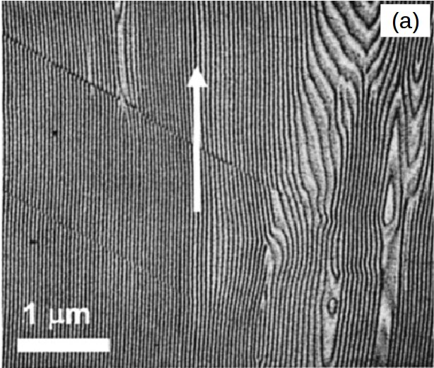
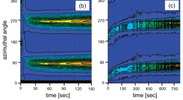
Figure 3: (a) TEM image of PS-b-PHEMA-b-PMMA triblock copolymer aligned from a THF solution in electric field of $E=1.8$ V$/\mu$m. Arrow indicates the field’s direction. Adapted from Ref. Boker et al. (2002b). (b) in-situ SAXS time-sequence pattern from a copolymer solution as a function of azimuthal angle in the plane perpendicular to the beam’s direction. The electric field is perpendicular to the beam. Angles of $0$ and $180$ degrees indicate lamellae perpendicular to the field; lamellae are parallel to ${\bf E}$ at $90$ and $270$ degrees. (b) and (c) are for system close and far from ODT point, respectively. Adapted from Ref. Boker et al. (2003).

The orientation dynamics has been studied as well. For a structure confined in a thin film, experiments Xu et al. (2005); Wang et al. (2006); Liedel et al. (2012) and numerical calculations Lyakhova et al. (2006); Kyrylyuk and Fraaije (2006) showed that lamellae or cylinders first form parallel to the substrate due to interfacial interactions. For a strong enough electric field they orient parallel to the field; they do so via two main pathways shown in the scattering patterns in Fig. 3 (b)-(c): the first one is partial melting, where small regions melt and then recrystallize and grow with the preferred orientation (Fig. 3 (b)). This mechanism is dominant for temperatures or compositions close enough to the order-disorder boundary in the phase diagram. The second mechanism is grain orientation, where large grains orient as a whole in the direction parallel to the field without melting first. This occurs far from the coexistence line and in systems that are not too viscous (Fig. 3 (c)).

Due to dielectric anisotropy ordered phases in electric field tend to orient such that dielectric interfaces perpendicular to the field are minimized, reducing the energy penalty in Eq. (21). A perfect lamellar stack or an hexagonal array of cylinders can reduce this energy to zero. But in other phases, such as the BCC lattice of spheres or the gyroid phase, this cannot happen. Once the soft crystal attains its optimal orientation, an increase of the field leads to stretching of domains in the direction parallel to the field. The actual deformation is dictated as a balance between electrostatic and elastic forces. At a critical field the energy of the deformed phase is too high and an order-order phase transition occurs accompanied by a change in the crystal’s symmetry. In block copolymers a sphere-to-cylinders was predicted theoretically by Tsori et al. Tsori et al. (2003b) and was verified experimentally by Xu et al. Xu et al. (2004) and by Giacomelli el. Giacomelli et al. (2010). Ensuing work considered the bulk phase diagram Tsori et al. (2006) and the sphere-to-cylinder transition in thin films Matsen (2006). Other order-order transitions are possible and may be technologically interesting, for example the gyroid-to-cylinder transition. This transition was studied theoretically Ly et al. (2007); Pinna and Zvelindovsky (2008), and experimentally with emphasis on surface effects Crossland et al. (2010).

IV Dielectric liquids in electric field gradients

As we mentioned above, variations in the composition of a mixture lead to variations of the electric field. We therefore define nonuniform fields as the fields that the electrodes confining the system would produce if the dielectric constant were spatially uniform. Such fields occur in fact only in highly idealized systems where the region of interest is infinitely smaller than the electrodes; field gradients are inevitable when the electrode size is comparable to the system size under investigation. When the field has gradient, Eq. (2) shows that there is a dielectrophoretic force which tends to pull the liquid with high value of $\varepsilon$ to regions with high value of $E$ Pohl (1978); Sullivan et al. (2003, 2006); Leunissen et al. (2008). It is not surprising therefore that field gradients lead to composition gradients in an initially-homogeneous system. The composition gradients occur on the same scale as the electric field, which is usually macroscopic. It may be said that the “composition follows the field” since $\nabla\phi$ is roughly proportional to $\nabla E^{2}$.

The interesting phenomenon is that there is a critical field above which a sharp composition gradients appear Tsori et al. (2004). In this state the composition variations can be much steeper than the lengthscale characterizing the field. To see this imagine the liquid mixture whose free energy density is $f=f_{\rm m}+f_{\rm es}$ confined by the wedge capacitor. The wedge is a hypothetical system comprised of two flat conductors tilted with an opening angle $\beta$ between them and potential difference $V$. $r$ is the distance from the imaginary meeting point of the two electrodes; its minimal and maximal values are $R_{1}$ and $R_{2}$, respectively. The mixture is confined to a region far from the edges of the electrodes but field gradients exist due to opening of the electrodes. In this simple system the field is in the azimuthal direction and its magnitude is given by $E=V/(\beta r)$. Close to the critical point one may use the expansions in small $\varphi=\phi-\phi_{c}$ as in Eqs. (17) and (18). In equilibrium the mixture’s profile is given by the Euler-Lagrange equation

$$f_{\rm m}^{\prime}(\varphi)=\frac{1}{2}\varepsilon^{\prime}\left(\frac{V}{\beta r}\right)^{2}+\mu.$$ (22)

Here we used a prime to denote denote differentiation with respect to $\varphi$ and assumed that $\varepsilon^{\prime\prime}=0$ to demonstrate a demixing phase transition that would not occur if the field were uniform.

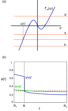
Figure 4: (a) Graphical solution to Eq. (22). Solid curve is $f_{\rm m}^{\prime}(\varphi)$. Its roots are the transition (binodal) compositions. The intersection between $f_{\rm m}^{\prime}(\varphi)$ and the horizontal dashed line gives the solution $\varphi(r)$ to Eq. (22). For voltages $V$ below the critical value $V^{*}$, the dashed line is bounded by lines a and b, corresponding to the the maximal and minimal values of the right-hand side of Eq. (22), giving rise to a continuous profile $\varphi(r)$. At $V>V^{*}$, line b is displaced to b’, and the intersection is at $\varphi<0$ for large $r$’s and at $\varphi>0$ at small $r$’s. (b) Qualitative composition profiles $\phi(r)$. Horizontal dashed line is the average composition $\phi_{0}$ in the absence of field. $\phi(r)$ varies smoothly when $V<V^{*}$, and has a sharp jump at $r=R$ when $V>V^{*}$.

The solution to this equation can be obtained graphically with the simplifying assumption that $f_{\rm m}$ from the expansion in Eq. (17) has only quadratic and quartic terms in $\varphi$. When the temperature is above $T_{c}$, $f^{\prime}_{\rm m}(\varphi)$ behaves similar $\varphi+\varphi^{3}$, namely it is monotonically increasing. Therefore, as the coordinate $r$ moves from large to small value the right hand side of the equation, being independent on $\varphi$, increases monotonically and $\varphi(r)$ accordingly changes continuously with $r$.

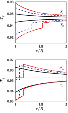
Figure 5: Diagonal elements of the stress tensor $T_{\rm rr}$ and $T_{\rm\theta\theta}$ for vapor-liquid coexistence in electric field gradients in (a) wedge capacitor and (b) charged wire. In both (a) and (b) the smallest radius is $R_{1}$. Horizontal dashed line corresponds to the pressure $p_{0}$ in the absence of external potential. At small potentials the density of the fluid is larger close to the inner radius and the stress is smoothly varying (black lines). At potentials above the critical value a demixing transition occurs and the pressures become discontinuous across the vapor-liquid interface (blue dashed lines). At even a larger potential the interface moves to larger values of $r$ (red dash-dot curves). Adapted from Ref. Samin and Tsori (2011a).

The situation is different at temperatures $T$ smaller than $T_{c}$. Here $f_{\rm m}$ behaves qualitatively as $-\varphi+\varphi^{3}$ as is shown in Fig. 4a. When the field, or external potential, is too small, the right-hand side of Eq. (22) is a horizontal line bounded between lines a and b, corresponding to the smallest and largest electric fields in the wedge. The resultant profile $\varphi(r)$ is then similar to the $T>T_{c}$ case. But his behavior is true only for small potentials; there exist a critical potential $V^{*}$ above which b is displaced to b’. In this case the solution to Eq. (22) jumps from the left branch of $f^{\prime}_{m}(\varphi)$ (negative values of $\varphi$) to the right branch (positive values of $\varphi$) discontinuously as $r$ decreases from large to small values. The demixing transition is then marked by a composition front whose thickness is much sharper than any length characterizing the field. At this state two phases coexist; both phases are nonuniform and the more polar one is located at the region of high electric field (small value of $r$).

IV.1 The pressure tensor and surface tension in vapor-liquid coexistence

Electric field gradients modify the coexistence of pure fluids too. “Electro-prewetting” occurs where an initially homogeneous vapor phase is brought under the influence of an electric field with gradients. For small gradients the molecules of the vapor are attracted to the region with large field and the density becomes larger there. At the critical voltage or field, the density becomes so large that liquid condenses with a well-defined liquid-vapor interface. This electroprewetting transition is different from sedimentation or condensation of particles in an external gravitational field or in centrifugation because, as mentioned above, in electric fields a small change in the composition or density affects the electric field even far away whereas the gravitational field is unaffected by the internal rearrangements of the liquid.

Another simple system that allows analytical development, besides the wedge, is a charged wire. For an infinitely long wire the system is effectively two dimensional and depends on $r$ and on $\theta$. If azimuthal symmetry is preserved the system becomes effectively one-dimensional and the field oriented in the radial direction. If a wire of radius $R_{1}$ inside a container with density and pressure corresponding to the vapor phase is charged at small voltage, the fluid density increases at the vicinity of the wire. At large enough wire voltage a liquid phase will precipitate near the wire, coexisting with the vapor phase far from it.

In Fig. 5 we show the stress tensor as calculated for the wedge (a) and wire (b) cases. The two diagonal components $\overleftrightarrow{T}_{\rm rr}$ and $\overleftrightarrow{T}_{\rm\theta\theta}$ are shown vs scaled distance from the origin ($\tilde{r}=r/R_{1}$). In both panels dashed lines correspond to small potentials, solid lines are potentials sufficient for demixing, and dash-dot lines are even larger potentials. For the last two cases an interface is created by the field separating the liquid and vapor phases. After the phase transition occurs, the stress tensor is discontinuous in $r$ (the body force is continuous though).

An important difference between the wedge and the wire is that once the interface is created, in the wedge the electric field is tangential to the interface whereas in the wire the electric field is normal to the interface. This is evident in the plots – in the wedge the $\theta\theta$ component of the pressure ($-\overleftrightarrow{T}_{\theta\theta}$) is smaller than the $rr$ component while in the wire $p_{\theta\theta}$ is larger than $p_{rr}$. In both the pressure inside the liquid drop (small $r$’s) is smaller than outside, quite different from the “regular” pressure of droplets as given by Laplace’s equation.

IV.2 Demixing dynamics in liquid mixtures

The dynamics of field-induced phase separation can be described by a modified “model H” framework. In this model the total flux is the sum of an advection term and a thermodynamic flux which is a gradient of the mixture’s chemical potential. This reaction-diffusion equation is accompanied by Navier-Stokes equation with a force depending on the field, and Laplace’s equation for the field. In some cases the symmetry dictates that hydrodynamic flow vanish identically or ${\bf u}$ is small enough and can be neglected, then the governing equations reduce to

$$\frac{\partial\phi}{\partial t} = L\nabla^{2}\frac{\delta f}{\delta\phi}~{},$$

$$\nabla\cdot(\varepsilon(\phi)\nabla\psi) = 0~{}~{},$$ (23)

where $L$ is a transport coefficient (assumed constant) and $\psi$ is the electrostatic potential (${\bf E}=-\nabla\psi$).

Figure 6 shows the stability diagram of a binary mixture confined in a cylindrical capacitor with inner and outer radii $R_{1}$ and $R_{2}$, respectively. The horizontal axis is the average mixture composition $\phi_{0}$. It is given for a specific value of the dimensionless electric field squared $M_{c}=\sigma^{2}v/(4k_{B}T_{c}\varepsilon_{0})$, where $\sigma$ is the surface charge density on the inner cylinder. Mixtures that are homogeneous in the absence of electric field were considered and hence only the area above the binodal curve $T_{b}(\phi_{0})$ is relevant. The shaded region is unstable with respect to the field applied, namely it has a sharp composition gradient. If a point $(\phi_{0},T)$ is outside of the shaded region the mixture still has composition variations but not a real interface. The unstable region is bounded by the binodal and by the lines marked 1 and 3. Point 2 is a surface critical point and line 1 is obtained as the locus of points 2 corresponding to electric field ($M_{c}$) increasing continuously from zero. Line 3 is the “electrostatic binodal”, for every temperature below that of point 2 its composition is the smallest for which an interface appears.

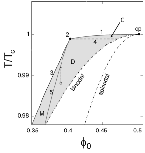
Figure 6: Schematic stability diagram of nonpolar binary mixtures in a cylindrical capacitor. Above the binodal curve composition variations exists; only in the shaded region the electric field is strong enough to induce a real interface (defined as a jump in $\phi(r)$ in the limit of vanishingly small $(\nabla\phi)^{2}$ term in the free energy). In region C the interface appears continuously (Fig. 7b) and in D it appears discontinuously (Fig. 7a). M is the metastable region. Point 2 is a surface critical point and cp is the critical point of the mixture in the absence of field. Adapted from Ref. Galanis and Tsori (2014a)

The unstable region can be further divided to three parts: M, D, and C Galanis and Tsori (2014b). At a fixed temperature above that of point 2, when the average composition $\phi_{0}$ increases and crosses line 1 into region C there is a continuous (second-order) transition where the equilibrium interface appears at a finite location $R$ intermediate between $R_{1}$ and $R_{2}$. The “jump” in $\phi$ across the interface, calculated in the sharp interface limit (i.e. without a $(\nabla\phi)^{2}$ term in the energy density Safran (1994)) vanishes at the transition line.

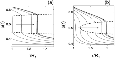
Figure 7: Composition profiles $\phi(r)$ for two regions (a) discontinuous, region D ($\phi_{0}=0.36$, $T/T_{c}=0.992$) and (b) continuous, region C ($\phi_{0}\simeq 0.4$, $T/T_{c}=0.997$) in Fig. 6. Each curve is a different snapshot in time taken at regular intervals on a logarithmic scale. Arrows indicate the direction of increasing time. Dashed lines indicate the composition where coexistence of two phases can exist based on a mixture free energy density $f_{\rm m}$ symmetric around $\phi=1/2$. In both parts $M_{c}=\sigma^{2}v/(4k_{B}T_{c}\varepsilon_{0})=0.069$ is the dimensionless field squared. Adapted from Ref. Galanis and Tsori (2014a)

In region D, separated from region C by the line 4, the transition is first order, namely when $\phi_{0}$ increases at fixed $T$ and crosses line 3 the equilibrium interface appears at the minimal radius $R=R_{1}$ and the jump in $\phi(R)$ is finite. The difference in equilibrium behavior leads to a different dynamics. Fig. 7 shows the profiles $\phi(r)$ calculated from Eqs. (23) at different times. The difference between the dynamics in region D (left) and C (right) is clearly seen when the interface appears at $R=R_{1}$ in D and at $R>R_{1}$ in C.

Line 5 is the “electrostatic spinodal” $\phi_{\rm es}(T)$ differentiating between D and M and defined by $f^{\prime\prime}(\phi_{0},T,r=R_{1})=0$. In D $f^{\prime\prime}(\phi_{0},r=R_{1})$ is always positive whereas in M $f^{\prime\prime}$ can be negative. The convexity of $f$ has a kinetic meaning. In region D the interface appears after a finite lag time $t_{L}$. The closer $\phi_{0}$ is to line 5 the longer the lag time is. The lag time diverges as a power law Galanis and Tsori (2014a)

$$t_{L}={\rm const.}\times(\Delta\phi)^{\alpha}$$ (24)

where $\Delta\phi=(\phi_{0}-\phi_{\rm es})/\phi_{\rm es}$ is the scaled distance from the electrostatic spinodal and $\alpha\simeq-1.16$ is the exponent. This relation holds irrespective of the value of $M_{c}$ as long as $\Delta\phi$ is small. In region M the system is metastable and phase separates only with sufficiently strong thermal noise or other nucleation event.

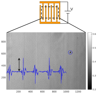
Figure 8: Representative phase contrast microscopy image from a mixture of ethyl lactate and squalene (2:8 v:v ratio) near interdigitated ITO electrodes (shown schematically above). The flat electrodes (thickness $\simeq 25$nm) is seen as vertical dark stripes; the gap is brighter. The polarity of the stripes is alternating between positive and negative. The relative brightness indicates the mixture’s composition. The voltage between adjacent electrodes was $700$V DC and the temperature was regulated by a Linkam LTS120E temperature stage to be $0.2^{\circ}$K above the binodal temperature. Colorbar shows the gray levels. Overlaid curve (blue) was obtained by subtraction of the gray levels (black=0, white=1) of the image and the ‘control’ (image without voltage), then averaging over the $y$-axis. Black arrow equals $0.3$ gray levels. Encircled dark spot is a dirty spot on the cover-slip glass and was not included in analysis. Images were cropped to size 1328x956.

To achieve phase separation with field gradients experimentally, the electrode setup is straightforward since strong field gradients occur in electrodes whose typical size is on the micrometer scale with voltages on the order of $\sim 100$V. The general design of a liquid cell consisted of standard $2.5$cm$\times 7.5$cm glass slide as the substrate, covered by a $2$cm$\times 2$cm cover slip. The liquid mixture was put in the $\sim 300\mu$m gap between the two layers. The edges of the cover slip were sealed by various glues or by a Teflon frame leading to actual cell size of $1.5$cm$\times 1.5$cm. Three types of electrodes were used. The first is wire electrodes, made from several metals with or without coating. Two wires were inserted into the cell prior to sealing and were connected to a DC or AC voltage supply. The wire’s radius varied from $50\mu$m to $200\mu$m. The field gradients results from the cylindrical symmetry around the wires. The second design consisted of a thin metallic coating on the bottom slide (Indium Tin Oxide, platinum, gold, silver or other metals) fabricated so as to have two “razor-blade” parts with a gap (width $\sim 50\mu$m) separating them. Here the field is mainly dictated by the thickness of the metallic layer ($\sim 25$nm) and not by the thickness of the gap. The field is largest close to the edges of the metal layer. In the third design the metallic layer had the shape of inter-digitated stripes in a comb-like manner. A voltage difference was imposed across any two adjacent stripes, as is schematically depicted in Fig. 8. The whole cell was put in a carefully controlled temperature chamber and was observed with phase-contrast optical microscopy. The large number of stripes and large sample area allows to infer the influence of small local defects and on the same time to obtain better statistics.

Images of the sample prior and after application of voltage were recorded and analyzed. Due to local irregularities of the electrodes and to enhance the detection of the separation, analysis was done only after subtraction of the ‘control’ image (corresponding to stable and thermally equilibrated sample without electric field). Fig. 8 is an example of a bare image. The blue superimposed curve is the gray level intensity averaged along the electrodes (y-direction) after the control image was subtracted.

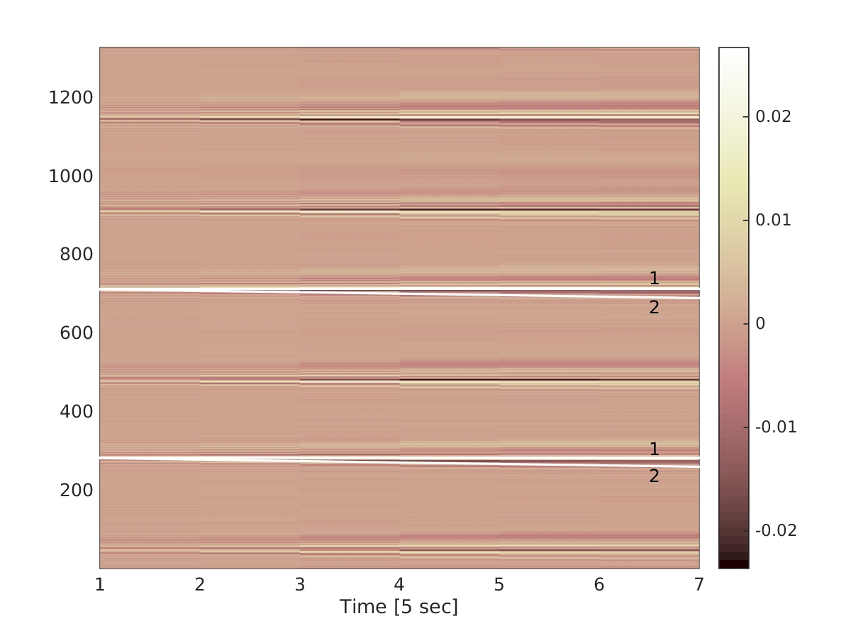
(a)

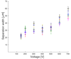
(b)

Figure 9: (a) Time progression of phase separation. Horizontal axis is time (in units of $5$sec) and vertical axis is the $x$-axis from Fig. 8. Colors indicate the gray levels of profiles such as the one overlaid in Fig. 8. White lines highlight the widening of the phase separation (only two pairs 1 and 2 are shown) – line 1 is horizontal and static and line 2 deviates from it, approximately linearly at early times. The gap between them is the width of the phase-separated region as a function of time. (b) The width of phase separated region at long times (15 mins) vs applied voltage. Measurements were taken from six different electrodes (different symbols). In (a) and (b) temperature, composition and other conditions are the same as in Fig. 8.

The time progression of such intensity curves is shown in Fig. 9a. The peaks and valleys of the curve in Fig. 8 correspond to red and blue tints, respectively. Out of the six edges shown in the images two were highlighted with white lines. The gap between them was defined as the thickness of the separated region. With increasing time the the phase separated regions near the edges of the electrodes widen.

The equilibrium thicknesses measured at long times are shown in Fig. 9b vs the applied voltage. For these liquids, mixture composition, and temperature, the thickness increases linearly with voltage until $V=300$V, it is approximately constant in the range $300$V-$500$V and increases again for $V>500$V. The plateau in intermediate voltages cannot be explained by the simple theory used so far.

The simple theory based on model B dynamics predicts that if the point $(\phi_{0},T)$ lies in region D of the stability diagram, Fig. 6, then there is a lag time for the phase separation depending on the distance from the “electrostatic spinodal”, line 5. Such lag time was observed experimentally as is shown in Fig. 10 for several temperatures above the field-free binodal curve $T_{b}$. For small values of $\Delta T=T-T_{b}$, the lag time is negligible compared to the error bars, recalling that the phase separation is quite faint and the onset of separation is not easy to detect. When $T$ increases closer to the “electrostatic binodal”, $\Delta T\simeq 1^{\circ}$K, the lag time increases markedly. Despite the many obvious qualitative and quantitative differences between the experimental and theoretical phase diagrams and the shortcomings of the theory, it seems that the temperatures of Fig. 10 roughly correspond to the dashed vertical arrow in Fig. 6 and therefore they validate the theoretical lag time concept.

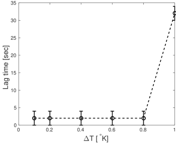
Figure 10: Lag time for the appearance of phase separation vs temperature difference $\Delta T=T-T_{b}$. Increasing values of $\Delta T$ corresponds qualitatively to the upward pointing dashed arrow in Fig. 6. The largest $\Delta T$ the closest $T$ is to the electrostatic binodal (line 5) and the larger the lag time is. The mixture of ethyl lactate and squalene with compositions 2:8 v:v was subject to $400$V on interdigitated electrodes.

V Demixing in polar solutions

In Sec. II.2 we discussed how, when two well defined phases are subject to electric fields, even a small amount of ions leads to marked differences as compared to pure dielectrics. The same is true when the initial state is mixed and there is no interface. In purely dielectric liquids the prewetting transition discussed in Sec. IV is induced by a dielectrophoretic force and this force arise only in nontrivial electrode geometries (i.e. curved or finite size), and not in one dimensional systems. However, when ions exist field gradients due to screening occur irrespective of the geometry. The lengthscale associated with the field is no longer the typical electrode size, $~{}\sim 1\mu$m, but rather the Debye screening length $\lambda_{D}\sim 10$nm. Hence even small potentials of $\sim 0.1$V lead to large fields $E\sim V/\lambda_{D}=10^{7}$V/m.

But ions are not equally miscible in all solvents. Ionic specificity to liquids and surface has been known for a long time (See Marcus (2002); Onuki and Kitamura (2004); Onuki et al. (2011) and references therein). The ionic affinity to neutral or hydrophobic surfaces, the so-called Hofmeister series Kunz et al. (2004), influences many physical properties, such as the water-air surface tension Jungwirth and Tobias (2006); Levin (2009); Levin et al. (2009) Markovich et al. (2014, 2015). It plays a central role in the solubility of proteins and underpins the “salting out” effect Zhang and Cremer (2006), which is commonly used in protein separation techniques.

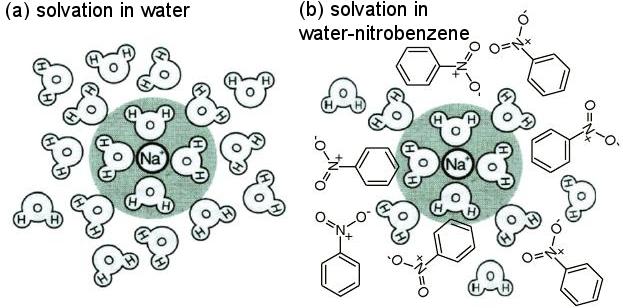
Figure 11: Schematic illustration of the solvation of Na⁺ in (a) pure water and (b) water-nitrobenzene. Water molecules are preferentially attached to the hydrophilic ion. The ion’s solvation energy is higher in (b) than in (a) and the difference exceeds the thermal energy. Adapted from Ref. Onuki and Okamoto (2011).

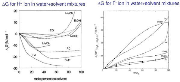
Figure 12: Gibbs transfer energy $\Delta G$ for moving an ion from pure water to mixtures with varying fractions of the co-solvent for H⁺ (left) and F^- (right) ions. Clearly the magnitude and trend (descending or ascending), or even the sign of the curves, is very ion-specific. Adapted from Ref. Hefter (2005).

Ionic specificity is even more pronounced in liquid mixtures. For example, in mixture of water and a less polar co-solvent, water molecules selectively attach to hydrophilic ions [see illustration in Fig. 11]. The typical difference in the solvation energy of an ion between solvents is typically of the order of $5$–$10k_{B}T$ per ion and can even be much larger. This Gibbs transfer energy strongly depends on both the solvents and the chemical nature of the ion Kalidas et al. (2000); Marcus (2007); Inerowicz et al. (1994); Osakai and Ebina (1998). Hence, the magnitude and sometimes the sign of the Gibbs transfer energy for cations and anions may differ greatly between mixtures Onuki and Okamoto (2011); Marcus (2002), as is seen in the curves of Fig. 12.

In the next two section we describe shortly two “applications” of liquid-liquid demixing in polar solutions.

VI Colloidal stabilization by addition of salt

Steric stabilization of colloids against the attractive van der Waals forces can be achieved using surfactant or polymer molecules that are physically or chemically attached to the colloid’s surface. Charged colloids can also be stabilized via the screened Coulomb repulsion, whose range depends on the Debye length $\lambda_{D}$. In the celebrated Derjaguin, Landau, Verwey, and Overbeek (DLVO) theory Derjaguin and Landau (1941); Verwey and Overbeek (1948), addition of salt to the suspension decreases the Debye length and the electrostatic repulsion leading eventually to coagulation and sedimentation of the colloids Russel et al. (1992).

In immiscible solvents selective solvation leads to a large ion partitioning between the liquid phases. This phenomenon underlies liquid-liquid extraction, a widely used separation method in chemical laboratories and in industry Hatti-Kaul (2000). But only few works investigate how selective solvation affects the interaction between charged surfaces. Leunissen et al. Leunissen et al. (2007a, b) and Zwanikken et al. Zwanikken and van Roij (2007) showed experimentally and theoretically that ion partitioning in an oil-water mixture can be used to tune the structure of colloidal suspensions and to produce additive-free water-in-oil emulsions that can crystallize.

Several studies investigated experimentally the interaction between charged surfaces in mixtures of partially miscible solvents Beysens and Estève (1985); Leunissen et al. (2007a); Hertlein et al. (2008); Nellen et al. (2011); Hopkins et al. (2009). In a binary mixture of water and 2,6-lutidine, a reversible flocculation of colloids occurs close to the demixing curve depending on the type and amount of salt Beysens and Estève (1985); van Duijneveldt and Beysens (1991); Law et al. (1998); Beysens and Narayanan (1999). It was only recently understood that selective solvation plays an important role in such experiments Ben-Yaakov et al. (2011); Zwanikken et al. (2008); Samin and Tsori (2011b); Okamoto and Onuki (2011) Samin and Tsori (2012); Bier et al. (2011); Sadakane et al. (2006, 2007) Sadakane et al. (2011, 2009) due to the non trivial electrostatics.

The bulk free energy density in polar mixtures is $f=f_{\rm m}+f_{\rm es}+f_{\rm ion}$, where the electrostatic $f_{\rm es}$ and ionic free energies are now Tsori and Leibler (2007); Ben-Yaakov et al. (2009)

$$f_{\rm es} = -\frac{1}{2}\varepsilon(\phi)(\nabla\psi)^{2}+(n^{+}-n^{-})e\psi~{},$$

$$f_{\rm ion} = k_{B}T[n^{+}\ln(v_{0}n^{+})+n^{-}\ln(v_{0}n^{-})]-(\Delta u^{+}n^{+}+\Delta u^{-}n^{-})\phi~{}.$$ (25)

Here $n^{\pm}$ are the ionic number densities and $\Delta u^{\pm}$ are the parameters proportional to the Gibbs transfer energies. This bilinear coupling of the ionic density to the mixtures composition is the lowest possible order for a generally complex interaction between the ions and mixture Bier et al. (2012). For a mixture confined by hard walls the surface energy density $f_{\rm s}$ is

$$f_{s}=\Delta\gamma\phi({\bf r}_{s})+\sigma\psi({\bf r}_{s}),$$ (26)

where ${\bf r}_{s}$ is a vector on the surface. The first term models the short-range interaction between the fluid and the solid. The parameter $\Delta\gamma$ measures the difference between the solid-water and solid-cosolvent surface tensions. The second term is the electrostatic energy for a surface with charge density $\sigma$.

Due to preferential solvation, when ions move to the electrodes they also “drag” the liquid in which they are better solvated, leading to a force of electrophoretic origin. Both electrophoretic ($\propto\Delta u$) and dielectrophoretic ($\propto\varepsilon^{\prime}$) forces lead to a phase separation transitions in liquid mixtures near charged surfaces. The window of temperatures above the binodal $\Delta T$ in which the mixture is unstable near one chemically-neutral ($\Delta\gamma=0$) wall charged at potential $V$, analogous to the difference between curve 3 and the binodal in Fig. 6, is given by Tsori and Leibler (2007)

$$\frac{\Delta T}{T_{c}}\simeq\left(\frac{|\varepsilon^{\prime}|}{\varepsilon_{c}}+\frac{\Delta u}{k_{B}T_{c}}\right)\frac{n_{0}v_{0}}{|\phi_{0}-\phi_{c}|}\exp\left(\frac{eV}{k_{B}T_{c}}\right)~{}.$$ (27)

Note the exponential dependence on $V$, rendering the demixing possible at virtually all temperatures above the binodal. The thickness of the demixing layer is a combination of the Debye length $\lambda_{D}$ and the correlation length of the mixture, and is of the order of $10$nm unless $T$ is very close to $T_{c}$.

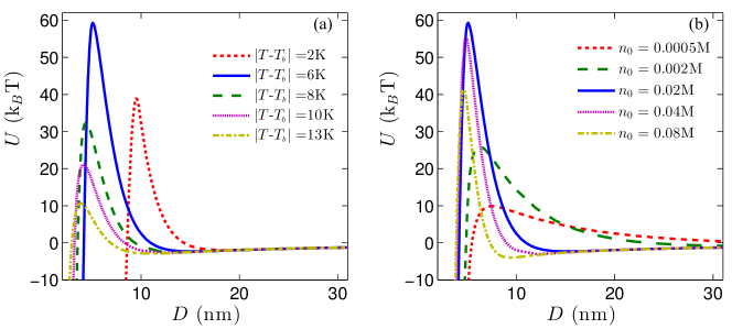
Figure 13: Theoretical effective potential $U(D)$ between two colloids with inter-surface separation $D$ immersed in a binary mixture with added antagonistic salt. The colloids repel at long distance and attract at short distance, with an energy barrier $U_{\rm max}$ at a distance $D_{\rm max}$. (a) Varying temperatures and fixed $n_{0}=20$mM (b) Varying salt amount and fixed $T=T_{b}+6$K. The location of the barrier at $D_{\rm max}$ decreases with increasing distance from the coexistence line $|T-T_{b}|$ or with increasing salt $n_{0}$ ($\lambda_{D}$ decreases). The surface of the colloids ($R=1\mu$m) was assumed hydrophobic and $\Delta u^{+}=-\Delta u^{-}=8k_{B}T$. Adapted from Ref. Samin et al. (2014).

Following the above insights it was suggested theoretically Samin and Tsori (2013) and recently established experimentally Samin et al. (2014) that colloids that otherwise coagulate and sediment in mixtures can be stabilized by the addition of salt. The key idea is this: suppose a hydrophobic particle is immersed in a mixture of water and a co-solvent. The co-solvent will partially wet the particle while water will be depleted. Antagonistic ions are ion pairs where the cation is hydrophilic and the anion is hydrophobic (or vice versa) Onuki and Kitamura (2004); Pousaneh and Ciach (2014). More generally, these are ions with a large difference in the Gibbs transfer energy, that is large $|\Delta u^{+}-\Delta u^{-}|$. If such ions are now added to the solution, the anions will be preferentially dissolved in the co-solvent (cation in the water) and hence the particles will be effectively charged and repelled from each other against van der Waals attraction. This repulsion is strong as long as the distance between them is not too small; at small separations the two co-solvent layers around the particle merge and capillary attraction together with van der Waals force become dominant leading to coagulation Samin et al. (2014).

How to calculate the effective potential between two colloids with surface-to-surface separation $D$? One employs the variation principle for the total free energy with respect to the four fields: mixture composition $\delta f/\delta\phi=0$, electrostatic potential $\delta f/\delta\psi=0$ (yielding the Poisson equation), and the two ionic densities $\delta f/\delta n^{\pm}=0$ (yielding the Boltzmann’s distribution for the ions). These equations are solved subject to the boundary conditions ${\bf n}\cdot\nabla\psi=\sigma/\varepsilon(\phi)$ and ${\bf n}\cdot\nabla\phi=-\Delta\gamma/C$, where ${\bf n}$ is the unit vector normal to the colloid’s surface, $\sigma$ is the surface charge density, $\Delta\gamma$ is the difference in the wettability of the two solvents at the colloid’s surface, and $C$ is the prefactor of the $(1/2)(\nabla\phi)^{2}$ term in the free energy density.

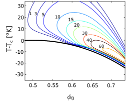
(a)

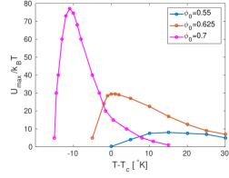
(b)

Figure 14: (a) A contour plot for the barrier height $U_{\rm max}$ in the $\phi_{0}$–$T$ plane in the Derjaguin’s approximation including vdW attraction for a colloid radius $R=1\mu$m. (b) Vertical cross-sections of part (a) are shown as curves of $U_{\rm max}$ vs T for three different compositions . At $\phi_{0}=0.55$ the potential barrier is shallow and almost independent on $T$. At $\phi_{0}$ the barrier has a strong $T$ dependence only at $T$ close to the critical temperature $T_{c}$, while at $\phi_{0}$ the curve is steep at all temperatures. Adapted from Ref. Samin and Tsori (2013).

Once the equilibrium profiles are found all thermodynamic quantities are known. The pressure tensor is $p_{ij}=-\overleftrightarrow{T}_{ij}=\left(\phi\delta f/\delta\phi+n^{+}\delta f/\delta n^{+}+n^{-}\delta f/\delta n^{-}-f\right)\delta_{ij}-\varepsilon E_{i}E_{j}$. The osmotic pressure is the difference between this expression and the bulk pressure, obtained when the composition and salt content equal their constant bulk values $\phi_{0}$ and $n_{0}$, respectively. If the distance between the colloids is smaller than their radius, $R\gg D$, the Derjaguin’s approximation can be applied in this manner: the potential $\Omega(D)$ is defined as the integral of the osmotic pressure from $D$ to $\infty$. Then the effective inter-colloid potential, including the simplest form of van der Waals interaction with a Hamaker’s constant $A$ is

$$U(D)=\pi R\int_{D}^{\infty}\Omega(D^{\prime})dD^{\prime}-\frac{AR}{12D}$$ (28)

The resultant potential $U(D)$ is shown in Fig. 13 for various temperatures and salt concentrations. In all curves repulsion exists at large distances. The potential attains a maximum at a distance $D_{\rm max}\approx 5$nm, $U_{\rm max}=U(D_{\rm max})$. At short enough distances $U(D)$ becomes attractive and the colloids will stick to each other. The above calculation assumes reasonable numbers, such as colloid radius $R=1\mu$m, Hamaker constant $A\sim 10^{-21}$J and antagonistic ions with $|\Delta u^{\pm}|=8$ (other values in the caption). The qualitative behavior stays the same irrespective of the exact numerical values. As can be seen on the left panel, the dependence on $T$ is non-monotonic for fixed salt content. As $T$ approaches the binodal temperature $T_{b}$, $D_{\rm max}$ increases while the maximum $U_{\rm max}$ increases and then decreases. The behavior is also non-monotonic for fixed $T$ and increasing salt content – in the right panel an increase in $n_{0}$ decreases $D_{\rm max}$ while $U_{\rm max}$ increases and then decreases. The location of the maximum at $D_{\rm max}$ is a nonlinear combination of the Debye length $\lambda_{D}$ and the correlation length of the mixture $\xi$.

One can map the value of $D_{\rm max}$ onto the phase diagram in the $\phi_{0}$–$T$ plane. Fig. 14a is such a contour plot for a fixed amount of added salt. The highest inter-colloid barrier and the most effective colloidal stabilization is found asymmetrically for values of $\phi_{0}$ greater than $\phi_{c}$ ($\phi_{c}=1/2$ in the model employed here) and for temperatures smaller than $T_{c}$. The experimental rule-of-thumb is that $U_{\rm max}$ needs to be larger than $\approx 3k_{B}$T in order to effectively prevent colloids from coagulation. The size of the area in the $\phi_{0}$–$T$ plane satisfying this requirement is generally large and independent of the exact numerical value of the parameters.

This non-DLVO stabilization mechanism has been tested with two types of binary mixtures: water–2,6 lutidine (LCST) and water–acetonitrile (UCST). Using dynamic light scattering, visible-light transmission spectroscopy, and cryo-TEM it was verified that graphene flakes were indeed suspended in water–acetonitrile mixtures with antagonistic salt (NaBPh₄, Na⁺ is hydrophilic, BPh${}_{4}^{-}$ is hydrophobic) but not with “regular” salt (NaCl, both ions are hydrophilic). Cross-linked polystyrene colloidal spheres were successfully suspended in water–2,6 lutidine mixtures with antagonistic salt but not with NaCl Samin et al. (2014).

An interesting opportunity arises for tuning the colloidal interactions with temperature. Fig. 14b shows the temperature dependence of the potential barrier height for three different mixture compositions $\phi_{0}$. In the first curve, $\phi_{0}=0.55$, the system behavior is expected to be virtually independent of $T$ since $U_{\rm max}$ is shallow for all values of $T$. One could, however, work with a mixture with $\phi_{0}\approx 0.62$ (orange curve). In this case the system will be insensitive to temperature variations as long as $T\gtrsim T_{c}+10$K (small slope) but will be quite sensitive at lower temperatures. The third curve ($\phi_{0}=0.7$, magenta) is further off-critical, and here the curve is steep at all values of $T$, meaning that the system’s stability is always sensitive to the temperature. The mixture composition is thus a valuable parameter for someone who wants to tune the stability of the dispersion against thermal variations between insensitive, partially sensitive, and sensitive. The additional boon of the method for certain applications is that the suspension is surfactant-free.

In the next section we investigate the role of electrostatics of liquid mixtures in pore filling transitions.

VII Pore filling transitions in membranes

Membranes in liquids are ubiquitous in Nature and in technology. The function of the membrane’s pore is to allow some species from one side to the other while blocking the rest Kedem and Katchalsky (1958); Jiang et al. (2002, 2003); Pendergast and Hoek (2011). It is advantageous to gate the pores to achieve better control of the dynamics and selectivity of the transport. Reversible pore gating has been achieved by temperature differences Yang and Yang (2003); Yameen et al. (2009). An alternative strategy, providing good anti-fouling properties, has recently been demonstrated in liquid-gated pores controlled by pressure variations across the membrane Hou et al. (2015). Electric potentials hold great promise because they they can be implemented in most systems, they can easily be turned on or off, and the voltages required are quite low: the field $E\sim V/\lambda_{D}$ is large even if $V$ small since $\lambda_{D}$ is on the nanometre scale. Indeed several works recently examined the effect of electric fields on the permeability of ions and solutes across the membranes and the influence on liquid-vapour coexistence near the pore Dzubiella et al. (2004); Dzubiella and Hansen (2005); Powell et al. (2011); Smirnov et al. (2011). In these works the existence of a transmembrane potential means that the direction of the field is parallel to the pore’s axis (and parallel to the pore walls).

A different direction for pore gating has been proposed recently, whereby the membrane is immersed in an aqueous mixture and the membrane is charged, leading to field in the direction perpendicular to the pore’s axis. For hydrophobic membranes, the pore opens and fills with water when voltage is applied to the membrane. The pore closes by filling with the co-solvent which diffuses in after the voltage is removed Samin and Tsori (2016). The filling transitions, expected to occur in both hydrophobic and hydrophilic membranes, can be triggered also by small changes in mixture composition or ambient temperature, and they can be continuous or abrupt. The role of preferential solvation of ions is crucial as it enables the transitions even for highly hydrophobic pores and at elevated temperatures above the critical temperature, unlike in regular capillary condensation Okamoto and Onuki (2010).

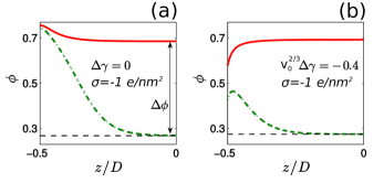
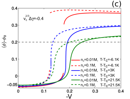
Figure 15: (a) Composition profile for chemically neutral ($\Delta\gamma=0$) and electrically charged ($\sigma\neq 0$) pore of width $D$ as a function of the transverse coordinate $z$ ($-D/2\leq z\leq D/2$). Only negative values of $z$ are shown since the pore is symmetric ($\phi(z)=\phi(-z)$). The cation and anion are both hydrophilic and calculation were done within the Modified Poisson-Boltzmann framework Borukhov et al. (1997). Dash-dot and solid curves are $\phi(z)$ just before and just after the filling composition. The horizontal dashed line is the bulk composition $\phi_{0}$. $\Delta\phi$, the difference between $\phi(z=0)$ and $\phi_{0}$, is vanishingly small before the filling transition and finite after it. (b) The same as in (a) but the pore is hydrophobic, $\Delta\gamma<0$. (c) Average water composition $\langle\phi\rangle$ in a hydrophobic pore vs negative pore potential $V$ (in Volts) for three different temperatures and two salt contents $n_{0}$. Adapted from Ref. Samin and Tsori (2016) (values of parameters therein).

The electrostatic potential, mixture composition, and ionic density profiles are calculated in the same manner as in Sec. VI, by employing the variational principle with respect to these fields, $\delta f/\delta\phi=0$, $\delta f/\delta\psi=0$, and $\delta f/\delta n^{\pm}=0$, where $f=f_{\rm m}+f_{\rm es}+f_{\rm ion}$, and $f_{\rm es}$ and $f_{\rm ion}$ are given in Eq. (VI) and the mixture energy $f_{\rm m}$ includes a $(1/2)C(\nabla\phi)^{2}$ term. The equations are solved subject to the boundary conditions derivable from the surface energy in Eq. (26): ${\bf n}\cdot\nabla\psi=\sigma/\varepsilon(\phi)$ and ${\bf n}\cdot\nabla\phi=-\Delta\gamma/C$.

The short-range preference of the pore wall to water or to the co-solvent leads to gradients in $\phi(z)$; surface charge density leads to gradients too. How to define then whether the pore is filled or not? Denoting $\Delta\phi$ as the difference between the mid-pore composition $\phi(z=0)$ and the bulk value $\phi_{0}$, before the filling transition $\Delta\phi\approx 0$ whereas after it $\Delta\phi$ is finite. Fig. 15 (a) shows $\phi(z)$ just before (dash-dot) and after (solid) the transition for a highly charged pore in a membrane that is neither hydrophilic nor hydrophobic. Both profiles are monotonously decreasing but the solid curve tends to $\approx 0.69>\phi_{c}$ in this case leading to a finite value of $\Delta\phi$. In part (b) of the Figure the corresponding profiles are shown with the change that now the pore is highly hydrophobic, as evidenced by the slope of both dash-dot and solid curves close to the left boundary ($z/D=-1/2$). The thickness of the adsorption layers in the curves corresponds to a modified Debye length $\lambda_{D}$ that depends on $n_{0}$, $\phi_{0}$, and $\Delta u^{\pm}$ Samin and Tsori (2016).

For porous carbonaceous membranes and other types of membranes one can control externally the surface potential within certain constraints. To quantify the filling transition as a function of external potential the average pore water composition is defined as $\langle\phi\rangle=(1/D)\int_{-D/2}^{D/2}\phi(z)dz$. The variation of $\langle\phi\rangle$ in a hydrophobic pore with increasing values of (negative) wall potential is shown in Fig. 15 (b) for two salt contents and three temperatures. At zero potential, water is depleted from the pore, $\langle\phi\rangle<\phi_{0}$. The water content increases with increasing $|V|$. Water is the majority in the pore once $\langle\phi\rangle-\phi_{0}$ exceeds $0.2$, since in this Figure $\phi_{0}=0.3$. The filling is continuous for the two high temperatures $T=T_{c}+21.5$K and $T=T_{c}+3$K and discontinuous at $T=T_{c}-6.1$K (the bulk mixture is homogeneous at this temperature). The voltage to (partially) fill the pore with water decreases with decreasing $T$ or with increasing $n_{0}$.

Pore filling occurs also in regular capillary condensation phenomena with short-range interactions. The selective solvation of the ions, being a volume contribution to the free energy, is dominant when either (i) the salt concentration is large, (ii) the membrane is highly charged, or (iii) the Gibbs transfer energy is large.

VIII Outlook

The dynamics and thermodynamics of liquids in electric fields is classical physics (pun intended). The elliptical nature of Laplace’s equation means that boundaries dictate the electric forces that occur remotely from them. Despite our old and tested knowledge of the mathematical formulae for the energy densities and the stresses, in complex, multi-component liquids, the system’s behavior is often difficult to predict or even describe. Enormous advances have been made in description of shape change, interfacial dynamics and related instabilities and the field is continuously evolving Melcher (1963); Bazant and Squires (2010); Chen (2011); Schnitzer and Yariv (2015); Rubinstein and Zaltzman (2015); Zwanikken and Olvera de la Cruz (2013); Onuki et al. (2016). We have highlighted how the preferential solvation of ions leads to forces that change dramatically the thermodynamics of liquid mixtures. This ingredient is expected to modify the classical models considerably. The addition of a new energy scale is especially intriguing in problems with time-varying fields where heating effects can be dominant. Researchers on these topics have plenty of work.

IX Acknowledgments

This work was supported by the European Research Council “Starting Grant” No. 259205, COST Action MP1106, and Israel Science Foundation Grant No. 56/14.

References

- Landau and Lifshitz (1957) L. D. Landau and E. M. Lifshitz, Elektrodinamika Sploshnykh Sred (Nauka, Moscow, 1957) chap. II, Sec. 18, problem 1.
- Melcher (1963) J. R. Melcher, Field-Coupled Surface Waves: A Comparative Study of Surface-Coupled Electrohydrodynamic and Magnetohydrodynamic Systems (M.I.T, 1963).
- Saville (1997) D. A. Saville, Annu. Rev. Fluid Mech. 29, 27 (1997).
- K. H. Panofsky and Phillips (2005) W. K. H. Panofsky and M. Phillips, Classical Electricity and Magnetism, 2nd ed. (Dover Publications, 2005).
- Herminghaus (1999) S. Herminghaus, Phys. Rev. Lett. 83, 2359 (1999).
- Pease and Russel (2002) L. F. Pease and W. B. Russel, J. Non-Newtonian Fluid Mech. 102, 233 (2002).
- Schaffer et al. (2000) E. Schaffer, T. Thurn-Albrecht, T. Russell, and U. Steiner, Nature 403, 874 (2000).
- Lau and Russel (2011) C. Y. Lau and W. B. Russel, Macromolecules 44, 7746 (2011).
- Lin et al. (2001) Z. Lin, T. Kerle, S. Baker, D. Hoagland, E. Schaffer, U. Steiner, and T. Russell, J. Chem. Phys. 114, 2377 (2001).
- Lin et al. (2002) Z. Lin, T. Kerle, T. Russell, E. Schaffer, and U. Steiner, Macromolecules 35, 3971 (2002).
- Wu et al. (2006) N. Wu, L. F. Pease, III, and W. B. Russel, Adv. Funct. Mater. 16, 1992 (2006).
- Goldberg-Oppenheimer and Steiner (2010) P. Goldberg-Oppenheimer and U. Steiner, Small 6, 1248 (2010).
- O’Konski and Thacher (1953) C. T. O’Konski and H. C. Thacher, J. Phys. Chem. 57, 955 (1953).
- Allan and Mason (1962) R. S. Allan and S. G. Mason, Proc. R. Soc. London, Ser. A 267, 45 (1962).
- Taylor (1966) G. I. Taylor, Proc. R. Soc. London, Ser. A 291, 159 (1966).
- Melcher and Taylor (1969) J. R. Melcher and G. I. Taylor, Annual Reviews of Fluid Dynamics 1, 111 (1969).
- Schaffer et al. (2001) E. Schaffer, T. Thurn-Albrecht, T. P. Russell, and U. Steiner, EPL 53, 518 (2001).
- Morariu et al. (2003) M. Morariu, N. Voicu, E. Schaffer, Z. Lin, T. Russell, and U. Steiner, Nature Materials 2, 48 (2003).
- Debye and Kleboth (1965) P. Debye and K. Kleboth, J. Chem. Phys. 42, 3155 (1965).
- Orzechowski (1999) K. Orzechowski, Chem. Phys. 240, 275 (1999).
- Wirtz and Fuller (1993) D. Wirtz and G. G. Fuller, Phys. Rev. Lett. 71, 2236 (1993).
- Beaglehole (1981) D. Beaglehole, J. Chem. Phys. 74, 5251 (1981).
- Early (1992) M. D. Early, J. Chem. Phys. 96, 641 (1992).
- Reich and Gordon (1979) S. Reich and J. M. Gordon, J. Polym. Sci., Part B: Polym. Phys. 17, 371 (1979).
- Kriisa and Roth (2014) A. Kriisa and C. B. Roth, J. Chem. Phys. 141, 134908 (2014).
- Amundson et al. (1994) K. Amundson, E. Helfand, X. Quan, S. D. Hudson, and S. D. Smith, Macromolecules 27, 6559 (1994).
- Tsori (2009) Y. Tsori, Rev. Mod. Phys. 81, 1471 (2009).
- Onuki and Fukuda (1995) A. Onuki and J. Fukuda, Macromolecules 28, 8788 (1995).
- Orzechowski et al. (2014) K. Orzechowski, M. Adamczyk, A. Wolny, and Y. Tsori, J. Phys. Chem. B 118, 7187 (2014).
- Amundson et al. (1991) K. Amundson, E. Helfand, D. D. Davis, X. Quan, S. S. Patel, and S. D. Smith, Macromolecules 24, 6546 (1991).
- Amundson et al. (1993) K. Amundson, E. Helfand, X. Quan, and S. D. Smith, Macromolecules 26, 2698 (1993).
- Pereira and Williams (1999) G. G. Pereira and D. R. M. Williams, Macromolecules 32, 8115 (1999).
- Tsori and Andelman (2002) Y. Tsori and D. Andelman, Macromolecules 35, 5161 (2002).
- Kyrylyuk et al. (2002) A. Kyrylyuk, A. Zvelindovsky, G. Sevink, and J. Fraaije, Macromolecules 35, 1473 (2002).
- Tsori et al. (2003a) Y. Tsori, F. Tournilhac, and L. Leibler, Macromolecules 36, 5873 (2003a).
- Tsori et al. (2006) Y. Tsori, D. Andelman, C.-Y. Lin, and M. Schick, Macromolecules 39, 289 (2006).
- Morkved et al. (1996) T. L. Morkved, M. Lu, A. M. Urbas, E. E. Ehrichs, H. M. Jaeger, P. Mansky, and T. P. Russell, Science 273, 931 (1996).
- Thurn-Albrecht et al. (2002) T. Thurn-Albrecht, J. DeRouchey, T. P. Russell, and R. Kolb, Macromolecules 35, 8106 (2002).
- Xu et al. (2003) T. Xu, C. J. Hawker, and T. P. Russell, Macromolecules 36, 6178 (2003).
- Xu et al. (2004) T. Xu, A. V. Zvelindovsky, G. J. A. Sevink, O. Gang, B. Ocko, Y. Q. Zhu, S. P. Gido, and T. P. Russell, Macromolecules 37, 6980 (2004).
- Boker et al. (2002a) A. Boker, H. Elbs, H. Hansel, A. Knoll, S. Ludwigs, H. Zettl, V. Urban, V. Abetz, A. H. E. Muller, and G. Krausch, Phys. Rev. Lett. 89, 135502 (2002a).
- Boker et al. (2003) A. Boker, H. Elbs, H. Hansel, A. Knoll, S. Ludwigs, H. Zettl, A. V. Zvelindovsky, G. J. A. Sevink, V. Urban, V. Abetz, A. H. E. Muller, and G. Krausch, Macromolecules 36, 8078 (2003).
- Boker et al. (2006) A. Boker, K. Schmidt, A. Knoll, H. Zettl, H. Hansel, V. Urban, V. Abetz, and G. Krausch, Polymer 47, 849 (2006).
- Schmidt et al. (2005) K. Schmidt, A. Boker, H. Zettl, F. Schubert, H. Hansel, F. Fischer, T. M. Weiss, V. Abetz, A. V. Zvelindovsky, G. J. A. Sevink, and G. Krausch, Langmuir 21, 11974 (2005).
- Schmidt et al. (2007) K. Schmidt, H. G. Schoberth, F. Schubert, H. Hänsel, F. Fischer, T. M. Weiss, G. J. A. Sevink, A. V. Zvelindovsky, A. Böker, and G. Krausch, Soft Matter 3, 448 (2007).
- Boker et al. (2002b) A. Boker, A. Knoll, H. Elbs, V. Abetz, A. Muller, and G. Krausch, Macromolecules 35, 1319 (2002b).
- Xu et al. (2005) T. Xu, A. V. Zvelindovsky, G. J. A. Sevink, K. S. Lyakhova, H. Jinnai, and T. P. Russell, Macromolecules 38, 10788 (2005).
- Wang et al. (2006) J.-Y. Wang, J. M. Leiston-Belanger, J. D. Sievert, and T. P. Russell, Macromolecules 39, 8487 (2006).
- Liedel et al. (2012) C. Liedel, M. Hund, V. Olszowka, and A. Boeker, Soft Matter 8, 995 (2012).
- Lyakhova et al. (2006) K. S. Lyakhova, A. V. Zvelindovsky, and G. J. A. Sevink, Macromolecules 39, 3024 (2006).
- Kyrylyuk and Fraaije (2006) A. V. Kyrylyuk and J. G. E. M. Fraaije, J. Chem. Phys. 125, 164716 (2006).
- Tsori et al. (2003b) Y. Tsori, F. Tournilhac, D. Andelman, and L. Leibler, Phys. Rev. Lett. 90, 145504 (2003b).
- Giacomelli et al. (2010) F. C. Giacomelli, N. P. da Silveira, F. Nallet, P. Cernoch, M. Steinhart, and P. Stepanek, Macromolecules 43, 4261 (2010).
- Matsen (2006) M. W. Matsen, J. Chem. Phys. 124, 074906 (2006).
- Ly et al. (2007) D. Q. Ly, T. Honda, T. Kawakatsu, and A. V. Zvelindovsky, Macromolecules 40, 2928 (2007).
- Pinna and Zvelindovsky (2008) M. Pinna and A. V. Zvelindovsky, Soft Matter 4, 316 (2008).
- Crossland et al. (2010) E. J. W. Crossland, S. Ludwigs, M. A. Hillmyer, and U. Steiner, Soft Matter 6, 670 (2010).
- Pohl (1978) H. A. Pohl, Dielectrophoresis: The Behavior of Neutral Matter in Nonuniform Electric Fields (Cambridge University Press, 1978).
- Sullivan et al. (2003) M. Sullivan, K. Zhao, C. Harrison, R. Austin, M. Megens, A. Hollingsworth, W. Russel, Z. Cheng, T. Mason, and P. Chaikin, J. Phys.: condens. Matter 15, S11 (2003), 5th Liquid Matter Conference, CONSTANCE, GERMANY, SEP 14-18, 2002.
- Sullivan et al. (2006) M. Sullivan, K. Zhao, A. Hollingsworth, R. Austin, W. Russel, and P. Chaikin, Phys. Rev. Lett. 96, 015703 (2006).
- Leunissen et al. (2008) M. E. Leunissen, M. T. Sullivan, P. M. Chaikin, and A. van Blaaderen, J. Chem. Phys. 128, 164508 (2008).
- Tsori et al. (2004) Y. Tsori, F. Tournilhac, and L. Leibler, Nature 430, 544 (2004).
- Samin and Tsori (2011a) S. Samin and Y. Tsori, J. Phys. Chem. B 115, 75 (2011a).
- Galanis and Tsori (2014a) J. Galanis and Y. Tsori, J. Chem. Phys. 141, 214506 (2014a).
- Galanis and Tsori (2014b) J. Galanis and Y. Tsori, J. Chem. Phys. 140, 124505 (2014b).
- Safran (1994) S. Safran, Statistical Thermodynamics of Surfaces, Interfaces, and Membranes (Westview Press, New York, 1994).
- Marcus (2002) Y. Marcus, Solvent Mixtures: Properties and Selective Solvation (CRC Press, 2002).
- Onuki and Kitamura (2004) A. Onuki and H. Kitamura, J. Chem. Phys. 121, 3143 (2004).
- Onuki et al. (2011) A. Onuki, R. Okamoto, and T. Araki, Bull. Chem. Soc. Jpn. 84, 569 (2011).
- Kunz et al. (2004) W. Kunz, J. Henle, and B. Ninham, Curr. Opin. Colloid Interface Sci. 9, 19 (2004).
- Jungwirth and Tobias (2006) P. Jungwirth and D. J. Tobias, Chem. Rev. 106, 1259 (2006), http://pubs.acs.org/doi/pdf/10.1021/cr0403741 .
- Levin (2009) Y. Levin, Phys. Rev. Lett. 102, 147803 (2009).
- Levin et al. (2009) Y. Levin, A. P. dos Santos, and A. Diehl, Phys. Rev. Lett. 103, 257802 (2009).
- Markovich et al. (2014) T. Markovich, D. Andelman, and R. Podgornik, Europhys. Lett. 106, 16002 (2014).
- Markovich et al. (2015) T. Markovich, D. Andelman, and R. Podgornik, J. Chem. Phys. 142, 044702.1 (2015).
- Zhang and Cremer (2006) Y. Zhang and P. S. Cremer, Curr. Opin. Chem. Biol. 10, 658 (2006).
- Onuki and Okamoto (2011) A. Onuki and R. Okamoto, Curr. Opin. Colloid Interface Sci. 16, 525 (2011).
- Hefter (2005) G. Hefter, Pure Appl. Chem. 77, 605 (2005).
- Kalidas et al. (2000) C. Kalidas, G. Hefter, and Y. Marcus, Chem. Rev. 100, 819 (2000).
- Marcus (2007) Y. Marcus, Chem. Rev. 107, 3880 (2007).
- Inerowicz et al. (1994) H. D. Inerowicz, W. Li, and I. Persson, J. Chem. Soc., Faraday Trans. 90, 2223 (1994).
- Osakai and Ebina (1998) T. Osakai and K. Ebina, J. Phys. Chem. B 102, 5691 (1998).
- Derjaguin and Landau (1941) B. V. Derjaguin and L. D. Landau, Acta Physicochim (USSR) 14, 633 (1941).
- Verwey and Overbeek (1948) E. J. W. Verwey and J. T. G. Overbeek, Theory of the Stability of Lyophobic Colloids (Elsevier, Amsterdam, 1948).
- Russel et al. (1992) W. B. Russel, D. A. Saville, and W. R. Schowalter, Colloidal Dispersions (Cambridge University Press, 1992).
- Hatti-Kaul (2000) R. Hatti-Kaul, Aqueous Two-Phase Systems (Humana Press, 2000).
- Leunissen et al. (2007a) M. E. Leunissen, A. van Blaaderen, A. D. Hollingsworth, M. T. Sullivan, and P. M. Chaikin, Proc. Natl. Acad. Sci. U.S.A. 104, 2585 (2007a).
- Leunissen et al. (2007b) M. E. Leunissen, J. Zwanikken, R. van Roij, P. M. Chaikin, and A. van Blaaderen, Phys. Chem. Chem. Phys. 9, 6405 (2007b).
- Zwanikken and van Roij (2007) J. Zwanikken and R. van Roij, Phys. Rev. Lett. 99, 178301 (2007).
- Beysens and Estève (1985) D. Beysens and D. Estève, Phys. Rev. Lett. 54, 2123 (1985).
- Hertlein et al. (2008) C. Hertlein, L. Helden, A. Gambassi, S. Dietrich, and C. Bechinger, Nature (London) 451, 172 (2008).
- Nellen et al. (2011) U. Nellen, J. Dietrich, L. Helden, S. Chodankar, K. Nygård, J. F. van der Veen, and C. Bechinger, Soft Matter 7, 5360 (2011).
- Hopkins et al. (2009) P. Hopkins, A. J. Archer, and R. Evans, J. Chem. Phys. 131, 124704 (2009).
- van Duijneveldt and Beysens (1991) J. S. van Duijneveldt and D. Beysens, J. Chem. Phys. 94, 5222 (1991).
- Law et al. (1998) B. M. Law, J.-M. Petit, and D. Beysens, Phys. Rev. E 57, 5782 (1998).
- Beysens and Narayanan (1999) D. Beysens and T. Narayanan, J. Stat. Phys. 95, 997 (1999).
- Ben-Yaakov et al. (2011) D. Ben-Yaakov, D. Andelman, R. Podgornik, and D. Harries, Curr. Opin. Coll. & Interface Sci. 16, 542 (2011).
- Zwanikken et al. (2008) J. Zwanikken, J. de Graaf, M. Bier, and R. van Roij, J. Phys.: Condens. Matter 20, 494238 (2008).
- Samin and Tsori (2011b) S. Samin and Y. Tsori, EPL 95, 36002 (2011b).
- Okamoto and Onuki (2011) R. Okamoto and A. Onuki, Phys. Rev. E 84, 051401 (2011).
- Samin and Tsori (2012) S. Samin and Y. Tsori, J. Chem. Phys. 136, 154908 (2012).
- Bier et al. (2011) M. Bier, A. Gambassi, M. Oettel, and S. Dietrich, EPL 95, 60001 (2011).
- Sadakane et al. (2006) K. Sadakane, H. Seto, and M. Nagao, Chem. Phys. Lett. 426, 61 (2006).
- Sadakane et al. (2007) K. Sadakane, H. Seto, H. Endo, and M. Shibayama, J. Phys. Soc. Jpn. 76, 113602 (2007).
- Sadakane et al. (2011) K. Sadakane, N. Iguchi, M. Nagao, H. Endo, Y. B. Melnichenko, and H. Seto, Soft Matter 7, 1334 (2011).
- Sadakane et al. (2009) K. Sadakane, A. Onuki, K. Nishida, S. Koizumi, and H. Seto, Phys. Rev. Lett. 103, 167803 (2009).
- Tsori and Leibler (2007) Y. Tsori and L. Leibler, Proc. Nat. Acad. Sci. 104, 7348 (2007).
- Ben-Yaakov et al. (2009) D. Ben-Yaakov, D. Andelman, D. Harries, and R. Podgornik, J. Phys.: Condens. Matter 21, 424106.1 (2009).
- Bier et al. (2012) M. Bier, A. Gambassi, and S. Dietrich, J. Chem. Phys. 137, 034504 (2012).
- Samin et al. (2014) S. Samin, M. Hod, E. Melamed, M. Gottlieb, and Y. Tsori, Phys. Rev. Appl 2, 024008 (2014).
- Samin and Tsori (2013) S. Samin and Y. Tsori, J. Chem. Phys. 139, 244905 (2013).
- Pousaneh and Ciach (2014) F. Pousaneh and A. Ciach, Soft Matter 10, 8188 (2014).
- Kedem and Katchalsky (1958) O. Kedem and A. Katchalsky, Biochim. Biophys. Acta 27, 229 (1958).
- Jiang et al. (2002) Y. Jiang, A. Lee, J. Chen, M. Cadene, B. Chait, and R. MacKinnon, Nature 417, 523 (2002).
- Jiang et al. (2003) Y. Jiang, A. Lee, J. Chen, V. Ruta, M. Cadene, B. Chait, and R. MacKinnon, Nature 423, 33 (2003).
- Pendergast and Hoek (2011) M. M. Pendergast and E. M. V. Hoek, Energy & Environmental Science 4, 1946 (2011).
- Yang and Yang (2003) B. Yang and W. T. Yang, J. Membr. Sci. 218, 247 (2003), 86.
- Yameen et al. (2009) B. Yameen, M. Ali, R. Neumann, W. Ensinger, W. Knoll, and O. Azzaroni, Small 5, 1287 (2009), 87.
- Hou et al. (2015) X. Hou, Y. Hu, A. Grinthal, M. Khan, and J. Aizenberg, Nature 519, 70 (2015), 10.
- Dzubiella et al. (2004) J. Dzubiella, R. J. Allen, and J. P. Hansen, J. Chem. Phys. 120, 5001 (2004).
- Dzubiella and Hansen (2005) J. Dzubiella and J. P. Hansen, J. Chem. Phys. 122 (2005), 10.1063/1.1927514.
- Powell et al. (2011) M. R. Powell, L. Cleary, M. Davenport, K. J. Shea, and Z. S. Siwy, Nature Nanotechnology 6, 798 (2011), 81.
- Smirnov et al. (2011) S. N. Smirnov, I. V. Vlassiouk, and N. V. Lavrik, Acs Nano 5, 7453 (2011).
- Samin and Tsori (2016) S. Samin and Y. Tsori, Colloid Interface Sci. Commun. 12, 9 (2016).
- Okamoto and Onuki (2010) R. Okamoto and A. Onuki, Phys. Rev. E 82, 051501 (2010).
- Borukhov et al. (1997) I. Borukhov, D. Andelman, and H. Orland, Phys. Rev. Lett. 79, 435 (1997).
- Bazant and Squires (2010) M. Z. Bazant and T. M. Squires, Current Opinion in Colloid & Interface Science 15, 203 (2010).
- Chen (2011) C.-H. Chen, in Electrokinetics And Electrohydrodynamics In Microsystems, CISM Courses and Lectures, Vol. 530, edited by A. Ramos (Springer-Verlag, Wien, 2011) pp. 177–220, conference on Electrokinetics and Electrohydrodynamics in Microsystems, Udine, ITALY, JUN 22-26, 2009.
- Schnitzer and Yariv (2015) O. Schnitzer and E. Yariv, J. Fluid Mech. 773, 1 (2015).
- Rubinstein and Zaltzman (2015) I. Rubinstein and B. Zaltzman, Phys. Rev. Lett. 114, 114502 (2015).
- Zwanikken and Olvera de la Cruz (2013) J. W. Zwanikken and M. Olvera de la Cruz, Proc. Nat. Acad. Sci. 110, 5301 (2013).
- Onuki et al. (2016) A. Onuki, S. Yabunaka, T. Araki, and R. Okamoto, Current Opinion In Colloid & Interface Science 22, 59 (2016).