Euclidean to Minkowski Bethe-Salpeter amplitude and observables

Abstract

We propose a method to reconstruct the Bethe-Salpeter amplitude in Minkowski space given the Euclidean Bethe-Salpeter amplitude – or alternatively the Light-Front wave function – as input. The method is based on the numerical inversion of the Nakanishi integral representation and computing the corresponding weight function. This inversion procedure is, in general, rather unstable, and we propose several ways to considerably reduce the instabilities. In terms of the Nakanishi weight function, one can easily compute the BS amplitude, the LF wave function and the electromagnetic form factor. The latter ones are very stable in spite of residual instabilities in the weight function. This procedure allows both, to continue the Euclidean BS solution in the Minkowski space and to obtain a BS amplitude from a LF wave function.

1 Introduction

Among the methods in quantum field theory and quantum mechanical approaches to relativistic few-body systems , the Bethe-Salpeter (BS) equation SB_PR84_51 , based on first principles and existing already for more than sixty years, remains rather popular.

The solution of the BS equation in Euclidean space is much more simple than in Minkowski one. Rather often the Euclidean solution is enough, mainly when one is interested in finding the binding energy. However, in many cases (e.g. for calculating electromagnetic (EM) form factors) one needs the Minkowski space amplitude or, equivalently, the Euclidean one with complex arguments Guernot_Eichmann . During the recent years, new methods to find the Minkowski solution for the two-body bound state were developed and proved their efficiency, at least for simple kernels like the one-boson exchange (OBE). Some of them KusPRD ; bs1 ; FrePRD12 ; fsv_2014 are based on the Nakanishi integral representation nakanishi of the BS amplitude and provide, at first, the Nakanishi weight function, which then allows to restore the BS amplitude and the light front (LF) wave function.

Other methods based on the appropriate treatment of the singularities in the BS equation, provide the Minkowski solution directly, both for bound and scattering states bs-long .

The straightforward numerical extrapolation of the solution from Euclidean to Minkowski space is very unstable and has not achieved any significant progress of practical interest. However, the above mentioned Nakanishi integral representation provides a more reliable method. It is valid for the Euclidean $\Phi_{E}$ as well as for the Minkowski $\Phi_{M}$ solutions and both solutions are expressed via one and the same Nakanishi weight function $g$. This integral representation, given in detail in the next section, can be symbolically written in the form:

$$\Phi_{E}=K_{E}\,g$$ (1)

and

$$\Phi_{M}=K_{M}\,g,$$ (2)

where $K_{E}$ and $K_{M}$ denote respectively the Nakanishi two-dimensional integral kernels in Euclidean and Minkowski spaces and g the weight function for the two-body bound state.

Solving the integral equation (1) relative to $g$ and substituting the result into relation (2), one can in principle determine the Minkowski amplitude $\Phi_{M}$ starting with the Euclidean one $\Phi_{E}$. This strategy seems applicable since, in contrast to the direct extrapolation $\Phi_{E}\to\Phi_{M}$, it uses the analytical properties of the BS amplitude which are implemented in the Nakanishi representation.

A similar integral relation exist expressing the LF wave function $\psi$ in terms of the Nakanishi weight function $g$ bs1 :

$$Ê\psi_{LF}=L\,g$$ (3)

One of the most remarkable interests of the Nakanishi representation is that it constitutes a common root for the three different formal objects $(\Phi_{E},\Phi_{M},\psi_{LF})$ allowing to determine any of them once known any other, and thus providing a link between two theoretical approaches – Bethe-Salpeter and Light-Front Dynamics – which are in principle and in practice quite different.

Since the LF wave function can be also found independently either by solving the corresponding equation cdkm (see for instance MC_2000 ) or by means of Quantum Field Theory (QFT) inspired approaches like the Discrete Light Cone Quantization Brodsky98 or the Basis Light Front Quantization approach vary2016 , one can pose the problem of finding the Nakanishi weight function from equation (3). This equation is only one-dimensional. Its solution is more simple, it requires matrices of smaller dimension and therefore it is more stable than the solution of the 2D equation (1).

It is worth noticing that the same method can be applied, far beyond the OBE dynamics, to the complete QFT dynamical content of the lattice calculations. Therein, the full (not restricted to the OBE kernel) Euclidean BS amplitude can be obtained and, via the Nakanishi integral, the corresponding BS amplitude in Minkowski space can be calculated as well as the observables. The Nakanishi representation was used in Craig to calculate the parton distribution amplitude for the pion.

The first results of our research in this field were published in FCGK . We have found that the solution of the integral equation (1) relative to $g$ was rather unstable. In order to find numerical solution, this integral equation was discretized using two quite different methods (Gauss quadratures and splines) and it resulted into a linear system. The instability of its the solution dramatically increases with the matrix dimension.

It turned out that the equation (1) is a Fredholm equation of the first kind, which mathematically a classical example of an ill-posed problem. On the other hand, this equation has a unique solution. The challenge here is to use an appropriate method allowing us to find this solution. These mathematical methods are developed and well known. Using them and knowing either $\Phi_{E}$ or $\psi_{LF}$ we aim to extract $g$ and find from it $\Phi_{M}$ and the corresponding observables. This will demonstrate that this procedure is feasible to get the solution.

The appearance of mathematically well defined but numerically ill-posed problems is not a rare exception. It is, for instance, manifested when using the Stieltjes and Lorentz integral transforms Efros_SJNP_1985 ; Efros:2007nq ; Giussepina_EFB23_2016 to solve the scattering few-body problems with bound state boundary conditions or when extracting the general parton distributions (GPD) from the experimental data Herve .

In this work we will proceed according to the following steps.

In a first step, we will solve numerically equations (1) and (3) in a toy model where $\Phi_{E}$, $\psi_{LF}$ and $g$ are known analytically. The comparison of the numerical solutions for $g$ with the analytical one will tell us the reliability of our method in solving the one dimensional and two-dimensional Fredholm first kind equations.

In a second step, we will go over a more realistic dynamical case. There, $\Phi_{E}$ is obtained by solving the Euclidean BS equation. The LF wave function is given by equation (3), where $g$ is calculated by using the methods introduced in bs1 , to solve the Minkowski BS equation, and based on the LF projection and Nakanishi representation. In order to keep trace of its origin we will denote it by $g_{M}$.

By solving equations (1) and (3), we find $g$ in two independent ways – denoted respectively $g_{E}$ and $g_{LF}$ – to be compared with each other as well as with $g_{M}$. Our methods should be consistent as far as all these weight functions are reasonably close to each other.

This wave function $\psi_{LF}$, found by projecting he BS amplitude in the light-front, and the $\psi_{LF}$ one obtained from solving the LF equation, are practically indistinguishable from each other. We find also the Minkowski BS amplitude $\Phi_{M}$ and using it, we calculate observables, namely, EM form factor and momentum distribution, represented by the LF wave function. We also calculate the form factor independently, expressing it via the LF wave function $\psi_{LF}$. It turned out that the form factors calculated by these two ways are very close to each other and practically insensitive to instabilities of $g$’s remaining after their suppression by the method we use. That demonstrates that indeed, knowing the Euclidean BS amplitude and using the methods developed in the present paper, one can calculate electroweak observables.

In Sec. 2 we present the formulas for the Nakanishi integral representation, both for the BS amplitude and the LF wave function. A change of variables (mapping) introduced to simplify the integration domain is described in Sec. 3. The numerical method for solving the discretized equation is presented in Sec. 4. The analytically solvable model, on which we will test the numerical solutions, comparing them with the analytical ones, is presented in Sec. 5. In Sec. 6 we study the stability of these solutions. In Sec. 7 we find numerically the Nakanishi weight function using as input the Euclidean BS amplitude and the LF wave function found from the OBE interaction kernel. These results are applied to calculate EM form factors in Sec. 8. Finally, Sec. 9 contains a genral discussion and the conclusions.

2 Nakanishi representation

The BS amplitude in Minkowski space $\Phi_{M}(k,p)$, for an $S$-wave two-body bound state with constituents masses $m$ ant total mass $M$, depends in the rest frame $p=(M,\vec{0})$ on two variables $k_{v}$ and $k_{0}$. We represent the four-vector $k$ as $k=(k_{0},\vec{k})$ and denote $k_{v}=|\vec{k}|$.

The Nakanishi representation for this amplitude reads nakanishi :

$$\Phi_{M}(k_{v},k_{0})=$$

$$\int_{-1}^{1}dz^{\prime}\int_{0}^{\infty}d\gamma^{\prime}\frac{g(\gamma^{\prime},z^{\prime})}{\left(\gamma^{\prime}+\kappa^{2}-k_{0}^{2}+k_{v}^{2}-Mk_{0}z^{\prime}-i\epsilon\right)^{3}}\,,$$

where $\kappa^{2}=m^{2}-\frac{M^{2}}{4}$ and $g$ is the Nakanishi weight function. The power of the denominator is in fact an arbitrary integer and we have chosen 3 for convenience. This is just the equation which is symbolically written in (2).

In the Euclidean space, after the replacement $k_{0}=ik_{4}$, this formula is rewritten as:

$$\Phi_{E}(k_{v},k_{4})=$$ (5)

$$\int_{-1}^{1}dz^{\prime}\int_{0}^{\infty}d\gamma^{\prime}\frac{g(\gamma^{\prime},z^{\prime})}{\left(\gamma^{\prime}+k_{4}^{2}+k_{v}^{2}+\kappa^{2}-iMk_{4}z^{\prime}\right)^{3}},$$

which was represented symbolically in (1).

One can also express through $g$ the LF wave function as bs1 :

$$\psi_{LF}(\gamma,z)=\frac{1}{4}\int_{0}^{\infty}\frac{(1-z^{2})g(\gamma^{\prime},z)d\gamma^{\prime}}{\Bigl{[}\gamma^{\prime}+\gamma+z^{2}m^{2}+\kappa^{2}(1-z^{2})\Bigr{]}^{2}}.$$ (6)

This equation corresponds to (3). As usually found in the literature, the LF wave function $\psi_{LF}$ is considered as depending on variables $k_{\perp}^{2},x$. They are related to $\gamma,z$ by $\gamma=k_{\perp}^{2},\;z=2x-1$ (see e.g. cdkm ).

The Euclidean BS amplitude $\Phi_{E}(k_{v},k_{4})$ can be easily found from the corresponding equation with a given kernel (OBE, for instance). As mentioned, it can be also found in lattice calculations BS_Latt , which are much difficult numerically but include all the Quantum Field Theory dynamics.

We remind, that alternatively to eq. (3) the LF wave function $\psi_{LF}$ can be found by solving a 2D equation in the LF dynamics cdkm or by using other QFT inspired methods like DLCQ Brodsky98 or BLFQ vary2016 .

We will therefore assume that one of the functions $\Phi_{E}$ or $\psi_{LF}$ is known and can be used as input for solving equations (5) or (6) relative to Nakanishi weight function $g$. Once obtained in this way, $g$ can be used to calculate any of the remaining quantities in the triplet $(\psi,\Phi_{E},\Phi_{M}$) and corresponding observables.

3 Mapping

Though, the time-like momentum variable varies in the range $-\infty<k_{4}<\infty$, we can reduce the problem to the half-interval $0<k_{4}<\infty$ and real arithmetic, by assuming $\Phi_{E}(k_{v},-k_{4})=\Phi_{E}(k_{v},k_{4})$. Furthermore, we will make in Eq. (5) the following mapping

$$0<\gamma^{\prime},k_{v},k_{4}<\infty\quad\to\quad 0<x^{\prime},x,z<1$$

by:

$$\gamma^{\prime}=\frac{x^{\prime}}{1-x^{\prime}},\quad k_{v}=\frac{x}{1-x},\quad k_{4}=\frac{z}{1-z}.$$ (7)

Eq. (5) takes then the form:

$$\Phi_{E}(x,z)=2\int_{0}^{1}dx^{\prime}\int_{0}^{1}dz^{\prime}\;\frac{g(x^{\prime},z^{\prime})}{(1-x^{\prime})^{2}}$$

$$\times \mbox{Re}\left[\frac{x^{2}}{(1-x)^{2}}+\frac{z^{2}}{(1-z)^{2}}+\frac{x^{\prime}}{1-x^{\prime}}+\kappa^{2}-iM\frac{zz^{\prime}}{1-z}\right]^{-3}.$$

to be solved in the compact domain $[0,1]\times[0,1]$. The factor $\frac{1}{(1-x^{\prime})^{2}}$ is the Jacobian. We rewrite this equation as:

$$\Phi_{E}(x,z)=\int_{0}^{1}dx^{\prime}\int_{0}^{1}dz^{\prime}\,K(x,z;x^{\prime},z^{\prime})g(x^{\prime},z^{\prime})$$ (9)

where

$$K(x,z;x^{\prime},z^{\prime})=\frac{2}{(1-x^{\prime})^{2}}$$

$$\times \mbox{Re}\left[\frac{x^{2}}{(1-x)^{2}}+\frac{z^{2}}{(1-z)^{2}}+\frac{x^{\prime}}{1-x^{\prime}}+\kappa^{2}-iM\frac{zz^{\prime}}{1-z}\right]^{-3}.$$

For the normal solutions $g(x^{\prime},-z^{\prime})=g(x^{\prime},z^{\prime})$ that comes from the symmetry of $\Phi_{E}$ with respect to $k_{4}$, which separates out the abnormal solutions for the two identical boson case.

After introducing in Eq. (6) for the variables $\gamma,\gamma^{\prime}$ the mapping defined in (7), we get that:

$$\psi_{LF}(x,z)=\int_{0}^{1}dx^{\prime}\,L(x,x^{\prime};z)g(x^{\prime},z)$$ (11)

where

$$L(x,x^{\prime};z) = \frac{(1-z^{2})}{4(1-x^{\prime})^{2}}$$

$$\times {\left(\frac{x}{1-x}+\frac{x^{\prime}}{1-x^{\prime}}+z^{2}m^{2}+\kappa^{2}(1-z^{2})\right)^{-2}}.$$

Here $z$ plays the role of a parameter.

4 Solving equations (9) and (11)

We will look for the solution of Eq. (9) by expanding it on Gegenbauer polynomials in both variables:

$$g(x,z)=\sum_{i,j=1}^{N_{x},N_{z}}c_{ij}G_{i-1}(x)G_{j-1}(z)$$ (13)

where

$$G_{n}(x)=\sqrt{2n+1}\,C^{\left(\frac{1}{2}\right)}_{n}(2x-1),$$ (14)

$C^{\left(\frac{1}{2}\right)}_{n}(2x-1)$ is a standard (non-normalized) Gegenbauer polynomial. Whereas, the polynomial $G_{n}(x)$ are orthonormalized:

$$\int_{0}^{1}dx\,G_{n}(x)G_{n^{\prime}}(x)=\delta_{nn^{\prime}}$$

We substitute $g(z,x)$ from (13) in Eq. (9), calculate the integrals numerically and validate the equation in $N=N_{x}\times N_{z}$ discrete points $(x_{i},z_{j})$, with $i=1,\ldots,N_{x}$ and $j=1,\ldots,N_{z}$. We chose as validation points $x_{i}$ ($z_{j}$) the $N_{x}$ ($N_{z}$) Gauss points in the interval $0<x<1$. Eq. (9) transforms into the following linear system:

$$\Phi_{ij}=\sum_{i^{\prime}j^{\prime}}^{N_{z},N_{x}}K_{ij}^{i^{\prime}j^{\prime}}c_{i^{\prime}j^{\prime}}$$ (15)

where

$$\Phi_{ij} = \Phi_{E}(x_{i},z_{j}),$$ (16)

$$K^{i^{\prime}j^{\prime}}_{ij} = \int_{0}^{1}dz^{\prime}\int_{0}^{1}dxK(x_{i},z_{j};z^{\prime},x^{\prime})G_{i^{\prime}-1}(x^{\prime})G_{j^{\prime}-1}(z^{\prime})$$

Eq. (15) is a $N\times N$ system of linear equations of the type $B=A\,C$ with the inhomogeneous term given by the euclidean BS amplitude $B\equiv\Phi_{ij}$ and as unknowns the array $C\equiv c_{ij}$ of coefficients of the expansion (13). The solution of this system $C=A^{-1}\,B$, will provide the coefficients $c_{ij}$ and by this the Nakanishi weight function $g(x,z)$ at any point.

The solution of Eq. (11) is found similarly. However, since $z$ is a parameter, the solution is found for a fixed $z$ and its decomposition is one-dimensional:

$$g(x,z)=\sum_{i=1}^{N}c_{i}G_{i-1}(x)$$ (17)

We substitute $g$ in Eq. (11), calculate the integral numerically and validate the equation in the $N$ Gaussian quadrature points $\{x_{j}\}$ in the interval $0<x<1$. Equation (11) transforms into the inhomogeneous linear system (the parameter $z$ is omitted):

$$\psi_{LF}(x_{j})=\sum_{i=1}^{N}L_{ji}\,c_{i},$$ (18)

where

$$L_{ji}=\int_{0}^{1}dx^{\prime}\,L(x_{j},x^{\prime};z)\,G_{i-1}(x^{\prime}),$$ (19)

with $L(x,x^{\prime};z)$ defined in (3). For a given $z$, the system (18) of $N$ linear equations is solved, and once determined the coefficients $c_{i}$, Eq. (17) provides the solution $g(x,z)$ everywhere.

Concerning the number of points $N$ used in the discretization of the integral equations there exists a ”plateau of stability”, corresponding to an optimal value of $N$. For a small values of $N$, the accuracy is not enough but, as we will see below, by increasing $N$ the solution becomes oscillatory and unstable. This is just a manifestation of above mentioned fact that the equations (9) and (11) represent both a Fredholm integral equation of the first kind which is a classical example of an ill-posed problem. Their kernels are quadratically integrable what ensures the existence and uniqueness of the solution. However, direct numerical methods do not allow to find the solution in practice, since they lead to unstable results. To avoid instability, one can, of course, keep $N$ small enough. However, for small $N$ the expansions (13) and (17) give a very crude reproduction of the unknown $g$. Therefore, to find solution, we will use a special mathematical method – the Tikhonov regularization (TRM) Tikhonov .

Note that another method (Maximum Entropy Method) was recently proposed MEM to solve Eq. (5) and successfully applied, at least in the case of monotonic $g$’s.

We will follow here the standard and straightforward way explained above: by discretization of the integral equation we turn it into a matrix equation and solve it by inverting the matrix, however, regularizing the inversion problem. The TRM Tikhonov allows to find a stable solution for sufficiently large $N$. Namely, following to Tikhonov , we will solve an approximate minimization problem, i.e., we will find $C$ providing the minimum of:

$$\parallel\,A\,C\,-\,B\,\parallel\,.$$

In the normal form, that corresponds to the replacement of the equation $A\,C\,=\,B$ by the regularized one $A^{{\dagger}}AC+\epsilon C=A^{{\dagger}}B$ with $\epsilon\ll 1$. The solution of this equation reads:

$$C_{\epsilon}=(A^{{\dagger}}A+\epsilon I)^{-1}A^{{\dagger}}B,$$ (20)

where $I$ is the identity matrix. For small $\epsilon$ (but not for infinitesimal) the solution $C_{\epsilon}$ of this equation is very close to the solution of the original equation $AC=B$. However, the solution of Eq. (20) is much more stable than the solution of $AC=B$.

In our previous work FCGK we also used a regularization procedure, but in a more naive form. The equation $AC=B$ was replaced not by $A^{{\dagger}}AC+\epsilon C=A^{{\dagger}}B$, but by $(A+\epsilon I)C=B$. Then, instead of the solution (20) we got

$$C_{\epsilon}=(A+\epsilon I)^{-1}B.$$ (21)

This increases the stability but not so strongly like (20), as we are going to illustrate in what follows.

5 Analytically solvable model

As the first step, we will check the methods and study the appearance of numerical instabilities by solving the simplest one-dimensional equation (6) in a model where the functions $\psi_{LF}$ and $g$ are known analytically. We will compare the numerical solution with the analytical one. In equation (6) the values $z,m$ and $\kappa$ are the parameters which can be chosen arbitrary (keeping the kernel non-singular). We can also put an arbitrary factor at the front of the integral in r.h.-side, which only changes the normalization of $\psi_{LF}$. Using this freedom, we choose $z^{2}m^{2}+\kappa^{2}(1-z^{2})=1$ and replace the factor $\frac{1}{4}(1-z^{2})$ also by 1. Then the equation (6) obtains the form:

$$\psi_{LF}(\gamma)=\int_{0}^{\infty}\frac{g(\gamma^{\prime})d\gamma^{\prime}}{(\gamma+\gamma^{\prime}+1)^{2}}.$$ (22)

As a solution we take:

$$g(\gamma)=\frac{1}{(1+\gamma)^{2}}$$ (23)

Its substitution it into (22) provides the l.h.-side:

$$\psi_{LF}(\gamma)=\frac{1}{\gamma^{3}}\left[\frac{\gamma(2+\gamma)}{(1+\gamma)}-2\log(1+\gamma)\right]$$ (24)

In the mapping variables the equation (22) is rewritten as:

$$\psi_{LF}(x)=\int_{0}^{1}L_{1}(x,x^{\prime})g(x^{\prime})dx^{\prime},$$ (25)

where the kernel $L_{1}$, the inhomogeneous term $\psi_{LF}$ and the solution $g$ read:

$$\psi_{LF}(x) = \Bigl{[}(2-x)x+2(1-x)\log(1-x)\Bigr{]}$$ (26)

$$\times \frac{(1-x)^{2}}{x^{3}},$$

$$L_{1}(x,x^{\prime}) = \frac{1}{\left[\frac{x}{1-x}+\frac{x^{\prime}}{1-x^{\prime}}+1\right]^{2}}\frac{1}{(1-x^{\prime})^{2}}$$ (27)

$$= \frac{(1-x)^{2}}{(1-xx^{\prime})^{2}},$$

$$g(x) = (1-x)^{2}.$$ (28)

We will consider $\psi_{LF}$, given by Eq. (26) as input, solve numerically, Eq. (25) in the form of the decomposition (17) and compare the solution with the analytical $g$ given in (28).

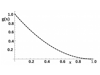
Figure 1: The numerical solution of Eq. (25) for $g(x)$ (dashed curve), found in the form of Eq. (17), for the discretization rank $N=11$ with $\epsilon=0$ in (21) in comparison to the exact solution $g(x)=(1-x)^{2}$ (not-distinguishable from the dashed curve).

6 Studying stability

In our precedent paper FCGK we have found that the inversion of the Nakanishi integral is rather unstable relative to the increase of the number of points $N$, using the regularization method given by Eq. (21). Therefore, solving Eq. (18), we will first study the onset of instability and its suppression by the Tikhonov regularization (20).

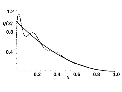
Figure 2: The same as in Fig. 1 but for $N=14$, $\epsilon=0$.

The solution of the non-regularized equation (18), by using Eq. (21) with $\epsilon=0$ and $N=11$, is shown in Fig. 1. It coincides, within the thickness of the lines, with the exact one, given by Eq. (28). However, when increasing $N$ up to $N=14$, we can observe (Fig. 2) the onset of instability: the numerical solution $g(x)$ becomes oscillating around the exact solution. Note also that the determinant of $A$ is very small and it quickly decreases when $N$ increases. For $N=11$, det$(A)\sim 10^{-35}$ while for $N=14$ one has det$(A)\sim 10^{-59}$.

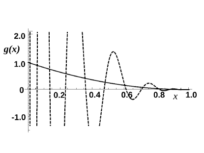
Figure 3: The same as in Fig. 1 but for $N=16$, $\epsilon=0$.

Further increase of $N$ results in extremely strong oscillations. The solution for $N=16$ and $\epsilon=0$, strongly oscillates and dramatically differs from the exact one, as it can be seen in Fig. 3 . For $N=32$ and $\epsilon=0$, the solution oscillates even more strongly and is wrong by orders of magnitude; we find for instance $g(0)\approx-10^{3}$ instead of $g(0)=1$ according to the analytic result.

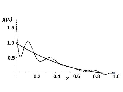
Figure 4: The same as in Figs. 1, 2, 3, but with Tikhonov regularization, for $N=16$ and $\epsilon=10^{-18}$.

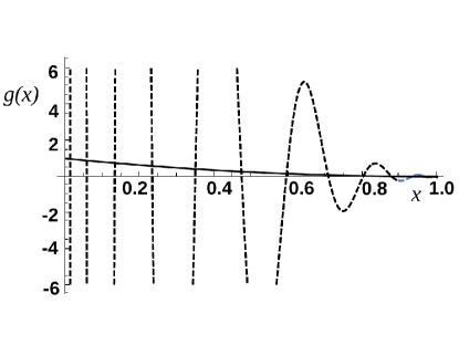
Figure 5: The same as in Fig. 4 but with the regularization by Eq. (21), $N=16$ and $\epsilon=10^{-10}$.

Now let us solve the corresponding equation by using TRM, Eq. (20). For $N=16$ and $\epsilon=10^{-10}$, we found that the oscillations completely disappear. The numerical solution coincides with the exact one within precision better than 1%, similarly to what we observe in the figure 1. To avoid repetition, we do not show the corresponding figure. For much smaller $\epsilon=10^{-18}$ with $N=16$, the solution found by TRM, Eq. (20), is shown in Fig. 4. It has some oscillations, which are strongly enhanced in the case with regularization (21) and $\epsilon=10^{-10}$. The same happens with the regularized solution for $N=14$, $\epsilon=10^{-10}$ (not shown), when we replace the Tikhonov regularization (20) by (21).

Our study shows that using the TRM method there is almost no $\epsilon$ dependence of the results in a rather wide limits. However, when $\epsilon$ is taken relatively large (e.g. $N=16$, $\epsilon=10^{-4}$), the numerical solution can sensibly differs from the exact one. On the other hand, as it was mentioned, when using too small $\epsilon$ one recovers the problem of oscillations, as it is seen in Fig. 4 ($N=16$ and $\epsilon=10^{-18}$). For $N=16,\epsilon=10^{-17}$ one can observe the first, yet weak signs of oscillations. Hence, for $N=16$, the stability (absence of oscillations) and insensitivity to the value of $\epsilon\neq 0$ are valid in rather large interval $\epsilon=10^{-4}\div 10^{-17}$.

The regularized solution for $N=32,\epsilon=10^{-10}$, found by Eq. (20) and TRM, again coincides with the exact one within thickness of lines. We do not show it since the curves are the same as in Fig. 1. For $N=32$, the oscillations appear at $\epsilon\leq 10^{-16}$.

For higher $N$ the situation is similar. Like in the case $N=32$, the solution for $N=64,\epsilon=0$, found by $C=A^{-1}B$ strongly oscillates and it strongly differs from the exact one, even stronger than in Fig. 3. The calculated value $g(0)\approx-10^{7}$ instead of $g(0)=1$ is again completely wrong. The regularized solution for $N=64,\epsilon=10^{-10}$, found by Eq. (20) also coincides with the exact one within thickness of lines, like it is in Fig. 1. However, the strong oscillations appear earlier, at $\epsilon\leq 10^{-13}$ (in contrast to $\epsilon\leq 10^{-16}$ for $N=32$).

We compare now the two ways of regularization given by Eqs. (21) and (20). In Fig. 5 the solution given by Eq. (21) for $N=16$, $\epsilon=10^{-10}$ is shown. It oscillates, while, the solution found by using TRM, Eq.(20), with same N and $\epsilon$ (not shown) coincides with the analytical one. As mentioned above, the solution for $N=16$ and $\epsilon=10^{-18}$ (Fig. 4) reveals moderate oscillations, which disappear at $\epsilon>10^{-17}$.

The reason which makes the determinant very small and turns the solution of the linear system in an ill-conditioned problem is the presence of very small eigenvalues of the kernel of the Fredholm integral equation (25). As the dimension of the matrix increases, more small eigenvalues are present, and the eigenstates are oscillating functions, that mixes with the solution obtained within a numerical accuracy. These contributions to the solution are oscillatory, building the pattern seen in Figs. 3 and 5, by increasing dimension of the matrix equation. The amplitude of the eigenvector contribution to the solution increases as the eigenvalue decreases, making the oscillations of the solution divergent. The regularization by $\epsilon$ cuts the contribution of the small eigenvalues, and to some extend the numerical stability can be found, at the expense of a finite $\epsilon$. Both regularization methods from Eq. (20) (Tikhonov method) and (21) improve the numerical solution. The Tikhonov regularization with the reduction to the normal form provides larger eigenvalues as compared to (21), as it is evident from the stability analysis that in practice allows much smaller $\epsilon$’s before considerable oscillations of the solution appear. See for example Fig. 5, where the method (21) provides huge oscillations. Whereas the TRM allows $\epsilon$ small as $10^{-18}$ compared with the solution with $\epsilon=10^{-10}$.

The calculations presented in this section demonstrate that the Nakanishi representation, at least, for the LF wave function, Eq. (6), can be indeed inverted numerically, that is, be solved relative to the Nakanishi weight function $g$. Though this representation, considered as an equation for $g$, is an ill-posed problem, special methods, in particular those based on the Tikhonov regularization (20), allows to solve it.

In the next section we will show that the Nakanishi representation (5) for the Euclidean BS amplitude can be also inverted. This will be shown not in a toy model, but for the BS solution with a OBE kernel.

7 OBE interaction

Let us now consider the dynamical case of two spinless particle of unit mass ($m=1$), interacting via OBE kernel with exchanged boson mass $\mu=0.5$, and forming a bound state of total mass $M=1.0$.

All the necessary solutions in this model – LF wave function $\psi_{LF}$, Euclidean BS amplitude $\Phi_{E}$ and Nakanishi weight function $g$ – have been computed by solving the corresponding equations. The weight function $g$ was found independently from the LF wave function and BS solutions by solving the equation derived in bs1 ; fsv_2014 with the same OBE kernel. We will use for $\psi_{LF}$ and $g$ the results fsv_2014 ; Gianni and for $\Phi_{E}$ – our own calculations.

We will take profit from the simplicity of the Euclidean solution and extract the Nakanishi weight function $g_{E}$ from $\Phi_{E}$ by inverting the Nakanishi representation in Euclidean space (5) via the Tikhonov regularization method and compare it with $g$ found from an equation derived from the Minkowski space BS equation fsv_2014 ; Gianni . The quality of the solution $g_{E}$ will be checked by computing the LF wave function $\psi_{LF}$ and comparing it with $\psi_{LF}$ found via $g$ provided by Gianni . Schematically the above extraction procedure is represented as $\Phi_{E}\to g_{E}\to\psi_{LF}$. Another possibility to extract $g$ is $\psi_{LF}\to g_{LF}\to\Phi_{E}$. Namely, starting with the LF wave function, get $g_{LF}$ and calculate with it the Euclidean $\Phi_{E}$ and compare this result with the initial $\Phi_{E}$. We will also compare the EM form factors calculated initially via $\psi_{LF}$ and, independently, via $\Phi_{M}$ and finally expressed via $g$. We will see that the observables are almost insensitive to the residual uncertainties in either $g_{E}$ or $g_{LF}$, which survive after suppressing the instabilities by the Tikhonov regularization (20). This ensures reliable results for the observables, when one uses the Euclidean BS amplitude as input, calculates $g$ by inverting the Nakanishi integral and then with the extracted $g$ goes to the observables.

The Nakanishi weight function $g_{E}$ obtained by inverting eq. (9) with $N_{x}=4,N_{z}=2$ and the TRM with $\epsilon=10^{-10}$, is shown in Fig. 6 (dashed line). Solid line represents the direct solution $g$ – denoted below as $g_{FSV}$ – computed in fsv_2014 ; Gianni by Frederico-Salmè-Viviani by solving a dynamical equation for $g$ and normalized in a different way than $\Phi_{E}$. To compare both solutions for $g$, we normalize $g_{E}$ so that the two solutions coincide (and equal to $-1$) at $x=0,\,z=0.3$.

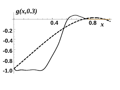
Figure 6: The solution $g_{E}(x,\,z=0.3)$ (dashed) found solving Eq. (9) with $N_{z}=2,N_{x}=4$ and $\epsilon=10^{-10}$, with $\Phi_{E}$, using the Tikhonov regularization method, compared to the solution $g_{FSV}(x,\,z=0.3)$ fsv_2014 ; Gianni (solid).

To check the quality of $g_{E}$, solution of Eq. (9), we substitute it in r.h.-side of Eq. (9), calculate $\Phi_{E}$ and compare it with the input $\Phi_{E}$. The result is shown in Fig. 7. We display by the solid curve the input Euclidean BS amplitude $c_{2}\,\Phi_{E}$ as a function of $x$ for a fixed value $z=0.3$. The dashed curve corresponds to the BS amplitude $\Phi_{E}(x,z=0.3)$ calculated via $g_{E}$ by Eq. (9). Up to a factor $c_{2}=0.88$ they are very close to each other.

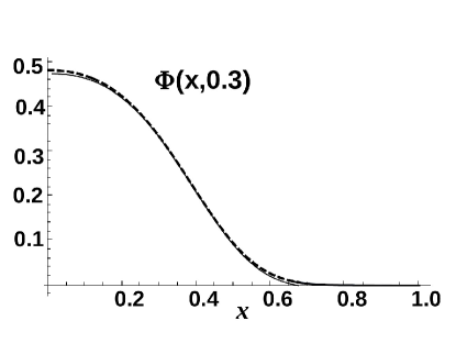
Figure 7: The solid curve corresponds to the Euclidean BS amplitude $c_{2}\,\Phi_{E}(z=0.3,x)$ ($c_{2}=0.88$) calculated via the BS equation with the OBE kernel. The dashed curve corresponds to the BS amplitude $\Phi_{E}(z=0.3,x)$ calculated via $g_{E}$ by Eq. (9).

The corresponding LF wave functions calculated from $g_{E}$ and $g_{FSV}$ by using Eq. (11) are shown in Fig. 8. We multiply $\psi_{LF}$ calculated by Eq. (11) by a normalization factor. Both $\psi_{LF}$’s well coincide with each other despite the difference between $g_{E}$ and $g_{FSV}$ seen in Fig. 6.

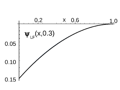
Figure 8: LF wave function calculated by Eq. (11) (multiplied by a normalization factor) for both extracted $g_{LF}$ and $g_{E}$ compared to the actual results obtained with $g_{FSV}$ in fsv_2014 ; Gianni from the Minkowski space solution of the BS equation. All the curves overlap with each other within the width of the lines.

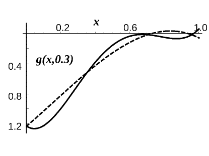
Figure 9: The Nakanishi weight function $g_{E}(x,z=0.3)$ extracted from $\Phi_{E}$, with $N_{z}=2,\,N_{x}=4$ (dashed curve) and $N_{x}=5,\,N_{z}=3$ (solid curve) with $\epsilon=10^{-10}$ using TRM.

The solution $g_{E}$ for $N_{x}=5$, $N_{z}=3$, $\epsilon=10^{-10}$ multiplied by a normalization factor, is shown in Fig. 9. For comparison, we add the solution for $N_{x}=4$, $N_{z}=2$, $\epsilon=10^{-10}$, shown by dashed line in Fig. 6. In spite of the visible difference between the dashed and solid curves, these two solutions give coinciding LF wave functions and the Euclidean BS amplitudes (after equivalent normalizations), similarly to ones shown in Figs. 7 and 8.

8 Calculating EM form factor

Once we have the Nakanishi weight function $g$ by Eqs. (2) and (6), we can find both the BS amplitude in Minkowski space and the LF wave function. The EM form factor can be expressed via both of them. In this way, we obtain two expressions in terms of $g$. We will use both to calculate the form factor and we will compare the results.

The electromagnetic vertex is expressed in terms of the BS amplitude by:

$$(p+p^{\prime})^{\nu}F^{BSM}(Q^{2})=i\int\frac{d^{4}k}{(2\pi)^{4}}\,(p+p^{\prime}-2k)^{\nu}$$ (29)

$$\times (k^{2}-m^{2})\Phi_{M}\left(\frac{1}{2}p-k;p\right)\Phi_{M}\left(\frac{1}{2}p^{\prime}-k;p^{\prime}\right),$$

where $Q^{2}=-q^{2}$, $q$ is the four-momentum transfer, and $p^{\prime}=p+q$. Substituting $\Phi_{M}$ in the form (2) and calculating the integral over $d^{4}k$, one gets (see Eq. (13) from ckm_2009 ):

$$F^{BSM}(Q^{2})=\frac{1}{2^{7}\pi^{3}N_{BSM}}\int_{0}^{\infty}d\gamma\int_{-1}^{1}dz\,g(\gamma,z)$$ (30)

$$\times \int_{0}^{\infty}d\gamma^{\prime}\int_{-1}^{1}dz^{\prime}\,g(\gamma^{\prime},z^{\prime})\int_{0}^{1}du\,u^{2}(1-u)^{2}\frac{f_{num}}{f^{4}_{den}}$$

with

$$f_{num} = (6\xi-5)m^{2}+[\gamma^{\prime}(1-u)+\gamma u](3\xi-2)$$

$$+ 2M^{2}\xi(1-\xi)+\frac{1}{4}Q^{2}(1-u)u(1+z)(1+z^{\prime})$$

$$f_{den} = m^{2}+\gamma^{\prime}(1-u)+\gamma u-M^{2}(1-\xi)\xi$$

$$+ \frac{1}{4}Q^{2}(1-u)u(1+z)(1+z^{\prime}),$$

where $\xi=\frac{1}{2}(1+z)u+\frac{1}{2}(1+z^{\prime})(1-u).$

The normalization factor $N_{BSM}$ is determined from the condition $F^{BSM}(0)=1$.

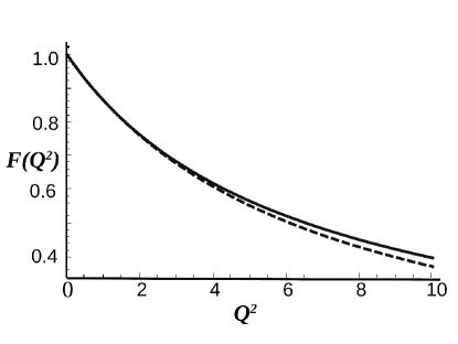
Figure 10: EM form factor calculated via LF wave function by Eq. (LABEL:FLFD), for $N_{z}=2,\;N_{x}=4$ (dashed curve) and for $N_{z}=3,N_{x}=5$ (solid curve), i.e., via solutions $g_{E}$ shown Fig. 9.

The form factor is expressed via LF wave function as follows (see e.g. Eq. (6.14) from cdkm ):

$$F^{LF}(Q^{2}) = \frac{1}{(2\pi)^{3}}\int\frac{d^{2}k_{\perp}dx}{2x(1-x)}$$ (31)

$$\times \psi_{LF}(\vec{k}_{\perp},x)\psi_{LF}(\vec{k}_{\perp}-x\vec{Q}_{\perp},x),$$

where ${\vec{Q}}_{\perp}^{2}=Q^{2}$. Substituting in (31) the LF wave function $\psi_{LF}(\vec{k}_{\perp},x)$ determined by Eq. (6), one finds (see Eq. (26) from ckm_2009 ):

$$F^{LF}(Q^{2})=\frac{1}{2^{5}\pi^{3}N_{LF}}\int_{0}^{\infty}d\gamma^{\prime}\int_{0}^{\infty}d\gamma\int_{0}^{1}dx\int_{0}^{1}du$$

$$\times \frac{x(1-x)\,u(1-u)\,g(\gamma,2x-1)g(\gamma^{\prime},2x-1)}{\left[u\gamma+(1-u)\gamma^{\prime}+u(1-u)x^{2}Q^{2}+m^{2}-x(1-x)M^{2}\right]^{3}}.$$

The EM form factor calculated via LF wave function by Eq. (LABEL:FLFD), for $N_{x}=4,\;N_{z}=2$ (dashed curve) and for $N_{x}=5,N_{z}=3$ (solid curve), i.e., via the solutions for $g_{E}$ given in Fig. 8, is shown in Fig. 10. We see that the apparently distinct solutions shown in Fig. 6 does not result in a considerable difference of the corresponding form factors. Notice that the differences represent only a 5% deviation at $Q^{2}\sim 10\,m^{2}$

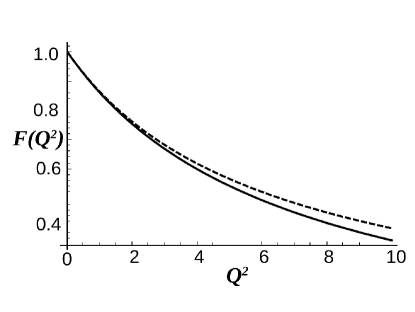
Figure 11: EM form factor calculated via Minkowski BS amplitude, by Eq. (30) with the same $g_{E}$ used to calculate the curves in Fig. 10; the curves are indicated as in Fig. 10.

The same form factor, calculated via the same Nakanishi weight functions, but in the Minkowski BS framework by Eq. (30) is shown in Fig. 11. The difference between the form factors corresponding to the two solutions for $g_{E}$ shown in Fig. 6 is larger than in Fig. 10, though it is still not so significant.

All four versions from Figs. 10 and 11 are shown for comparison together in Fig. 12. One can distinguish only three curves of the four since two of then coincide with each other. We compare form factors calculated via LF wave function and Minkowski BS amplitude using $g_{E}$. The form factor calculated via LF wave function by Eq. (LABEL:FLFD), for $N_{x}=5,\;N_{z}=3$ and calculated via Minkowski BS amplitude, by Eq. (30), for $N_{x}=4,\;N_{z}=2$ are shown by the solid line (upper curve). They are indistinguishable within thickness of lines.

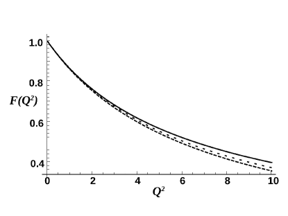
Figure 12: The EM form factor for the four calculations given in Figs. 10 and 11 with $g_{E}$ shown in Fig. 9. Solid (upper) curve: results obtained via LF wave function by Eq. (LABEL:FLFD), for $N_{x}=5,\;N_{z}=3$ and via Minkowski BS amplitude, by Eq. (30), for $N_{x}=4,\;N_{z}=2$, which are indistinguishable within thickness of the line. Dotted (middle) curve: results obtained via LF wave function by Eq. (LABEL:FLFD) for $N_{x}=4,\;N_{z}=2$. Dashed (bottom) curve: results obtained via Minkowski BS amplitude, by Eq. (30), for $N_{x}=5,\;N_{z}=3$.

It is worth to make the two following remarks. (i) Though the form factors $F^{LF}(Q^{2})$ and $F^{BSM}(Q^{2})$ turned out to be very close to each other (as it is seen from the present calculations and from ckm_2009 ), they should not coincide exactly. Their deviation seen in Fig. 12 is caused not only by numerical uncertainties, but also by physical reasons. This deviation cannot be completely removed by more precise calculations. From point of view of the Fock decomposition of the state vector, the form factor $F^{LF}(Q^{2})$ is determined only by the two-body contribution in the state vector, whereas $F^{BSM}(Q^{2})$, determined by the two-body BS amplitude, includes implicitly the effect of higher LF Fock states. (ii) The contribution of the higher Fock components can be found knowing only the two-body component. Indeed, inverting Eq. (6), we extract $g_{LF}$ from the two-body LF wave function $\psi_{LF}$. It is the same $g$ that enters in the Minkowski BS amplitude (2) and in the form factor (30), including the higher sector contributions.

As it was just mentioned, the form factor (30) (calculated with $g_{LF}$ extracted from the two-body LF wave function) includes implicitly not only the two-body component contribution but also the higher Fock components. So, this higher Fock sector contribution is found from the two-body component which was taken as input. Though it seems a little bit paradoxical (the possibility to get information about higher Fock states from the two-body one), this is, probably, a manifestation of self-consistency of the Fock decomposition embedded in the Nakanishi integral representation. In the field-theoretical framework (in which only the BS amplitude can be defined via the Heisenberg field operators SB_PR84_51 ), the number of particles is not conserved and the existence of one Fock component requires the existence of other ones. The set of them, corresponding to different numbers of particles, ensures also the correct transformation properties of the full state vector $|p\rangle$ since the Fock components are transformed by dynamical LF boosts in each other.

The fact that the difference between form factors determined by the two-body LF wave function and the form factor including higher components is small was found also in Wick-Cutkosky model dshvk . The contribution of many-body components with $n\geq 3$ reaches 36% in the full normalization integral $F(0)$ only for the coupling constant so huge that the total mass of the bound system tends to zero.

A final remark: the stability of the form factors obtained from $g_{E}$, though quite unexpected in view of the sizeable difference of the Nakanishi weight functions (see e.g. Fig. 8), is in fact appropriate. As we have discussed in the analytical example, the reason for the instability of the solution of the linear system is the contribution from the very small eigenvalues. Therefore the difference between the $g_{E}$’s comes from the corresponding eigenvectors which induce the observed oscillations. However, when using the Minkowski BS amplitude to compute the form factor, the contributions from the eigenvectors with small eigenvalues are damped in the same way they were enhanced in the inversion. It is very likely that this result follows from the fact that the spectra of the Nakanishi kernels in Minkowski and Euclidean spaces are the same.

9 Discussion and conclusion

We have demonstrated by explicit calculations, that the Nakanishi representations of the Bethe-Salpeter amplitude in Euclidean space ($\Phi_{E}$) and the light-front wave function ($\psi_{LF}$) can be numerically inverted. If one of this two quantities is known, one can easily calculate the other one as well as the Bethe-Salpeter amplitude in Minkowski space ($\Phi_{M}$) and associated observables, like the electromagnetic form factor.

We have developed an analytically solvable model, in the framework of which we compared the accuracy of the numerical solution with the analytical one. Though the inversion of a Fredholm integral equation of the first kind providing $g$ is an ill-posed problem, it can be solved with satisfactory precision by using appropriate methods.

Our best results are obtained with the Tikhonov regularization procedure. This method is rather efficient and it allowed to successfully overcome the instabilities of the solution which we found in a previous work FCGK when computed $g$ from $\Phi_{E}$. In addition, it turns out that the light-front wave function and observables are insensitive to the residual uncertainty of $g$ which remains after stabilizing the solution by the regularization. The uncertainties on the Light-Front wave function are within less than 1%, that is much smaller than for $g^{\prime}s$.

The Nakanishi weight function $g$ was expanded in terms of Gegenbauer polynomials. A small number of terms in this decomposition is required to control the instabilities. This method is very efficient for describing monotonic behaviors but it is not sufficient to reproduce more involved structure of $g$ like the ones provided by the dynamical model. The later ones generate considerable uncertainties in the inversion procedure. Increase of the number of terms in the decomposition gives more flexibility, but, at the same time, it enhances the numerical instability of the solution. We believe that it would be useful to study other basis or discretization methods, reflecting more the particular functional form of $g$.

Our approach can find interesting applications to extract Minkowski amplitudes from an Euclidean theory, like for instance Lattice QCD. The Euclidean BS amplitude is being currently computed there with the full dynamical contents of the theory. If one is able to extract from it the corresponding Nakanishi weight function $g$, one can access to time-like form factors, momentum distributions, GPD’s and TMD’s which are not accessible in a direct way. This could considerably simplify the study of the Minkowski space structure of hadrons from Lattice QCD ab-initio calculations.

References

- (1) E.E. Salpeter, H.A. Bethe, Phys. Rev. 84, 1232 (1951)
- (2) G. Eichmann, Few Body Syst. 57, (2016) 541 (2016); Phys. Rev. D 84, 014014 (2011)
-
(3)
K. Kusaka, A. G. Williams, Phys. Rev. D 51, 7026 (1995);
K. Kusaka, K. Simpson, A.G. Williams, Phys. Rev. D 56, 5071 (1997) -
(4)
V.A. Karmanov, J. Carbonell, Eur. Phys. J. A 27, 1 (2006);
J. Carbonell, V.A. Karmanov, Eur. Phys. J. A 27, 11 (2006) - (5) T. Frederico, G. Salmè, M. Viviani, Phys. Rev. D 85, 036009 (2012); Phys. Rev. D 89, 016010 (2014)
- (6) T. Frederico, G. Salmè, M. Viviani, Phys. Rev. D 89, 016010 (2014)
- (7) N. Nakanishi, Prog. Theor. Phys. Suppl. 43, 1 (1969); 95, 1 (1988)
- (8) J. Carbonell, V.A. Karmanov, Phys. Rev. D 90, 056002 (2014)
- (9) J. Carbonell, B. Desplanques, V.A. Karmanov, J.-F. Mathiot, Phys. Reports, 300 (1998) 215
- (10) M. Mangin-Brinet and J. Carbonell, Phys. Lett. B 474, 237 (2000)
- (11) S.J. Brodsky, H. Pauli, and S.S. Pinsky, Phys. Rep. 301, 299 (1998)
- (12) J. P. Vary, L. Adhikari, G. Chen, Y. Li, P. Maris and X. Zhao, Few Body Syst. 57, 695 (2016)
- (13) Lei Chang, I. C. Cloët, J. J. Cobos-Martinez, C. D. Roberts, S. M. Schmidt, and P. C. Tandy, Phys. Rev. Lett. 110, 132001 (2013)
- (14) T. Frederico, J. Carbonell, V. Gigante and V.A. Karmanov, Few-Body Syst. 56, 549 (2016)
- (15) V.D. Efros, Sov. J. Nucl. Phys. 41, 949 (1985)
- (16) V. D. Efros, W. Leidemann, G. Orlandini, and N. Barnea, J. Phys. G: Nucl. Part. Phys. 34, R459 (2007)
- (17) G. Orlandini, F. Turro, arXiv:1612.00322
- (18) C. Mezrag, H. Moutarde, J. Rodriguez-Quintero, Few Body Syst. 57, 729 (2016)
- (19) N. Ishii, S. Aoki, T. Hatsuda, Phys. Rev. Lett. 99, 022001 (2007)
- (20) Fei Gao, Lei Chang, Yu-xin Liub, arXiv:1611.03560 [nucl-th]
- (21) A.N. Tikhonov, A.V. Goncharsky, V.V. Stepanov, A.G. Yagola, Numerical Methods for the Solution of Ill-Posed Problems, Kluwer Academic Publishers, 1995
- (22) G. Salmè, private communication
- (23) J. Carbonell, V.A. Karmanov, M. Mangin-Brinet, Eur. Phys. J. A 39, 53 (2009)
- (24) Dae Sung Hwang and V.A. Karmanov, Nucl. Phys. B 696, 413 (2004)