Machine Learning of Linear Differential Equations using Gaussian Processes
Abstract
This work leverages recent advances in probabilistic machine learning to discover conservation laws expressed by parametric linear equations. Such equations involve, but are not limited to, ordinary and partial differential, integro-differential, and fractional order operators. Here, Gaussian process priors are modified according to the particular form of such operators and are employed to infer parameters of the linear equations from scarce and possibly noisy observations. Such observations may come from experiments or “black-box” computer simulations.
keywords:
probabilistic machine learning , differential equations , Gaussian processes , inverse problems , uncertainty quantification1 Introduction
A grand challenge with great opportunities facing researchers is to develop a coherent framework that enables scientists to blend conservation laws expressed by differential equations with the vast data sets available in many fields of engineering, science and technology. In particular, this article investigates conservation laws of the form
which model the relationship between two black-box functions and . Here,
| (1) |
and is a parametric linear operator identified by its parameters . Given noisy observations , of , , respectively, the aim is to learn the parameters and hence the governing equation which best describes the data. Such problems are ubiquitous in science, and in mathematical literature are often referred to as “inverse problems” (see [1, 2]). To provide a unified framework for resolving such problems, this work employs and modifies Gaussian processes (GPs) (see [3, 4]), which is a non-parametric Bayesian machine learning technique. Quoting Diaconis [5], “once we allow that we don’t know (and ), but do know some things, it becomes natural to take a Bayesian approach”. The Bayesian procedure adopted here, namely Gaussian processes, provides a flexible prior distribution over functions, enjoys analytical tractability, and has a fully probabilistic work-flow that returns robust posterior variance estimates which quantify uncertainty in a natural way. Moreover, Gaussian processes are among a class of methods known as kernel machines (see [6, 7, 8]) and have analogies with regularization approaches (see [9, 10, 11]). However, they are distinguished by their probabilistic viewpoint and their powerful traning procedure. Along exactly the same lines, the methodology outlined in this work is related to and yet fundamentally differentiated from the so-called “meshless” methods (see [12, 13, 14, 15]) for differential equations. Furthermore, differential equations are the cornerstone of a diverse range of applied sciences and engineering fields. However, use within statistics and machine learning, and combination with probabilistic models is less explored. Perhaps the most significant related work in this direction is latent force models [16, 17]. Such models generalize latent variable models [18, 19, 20] using differential equations. In sharp contrast to latent force models, this work bypasses the need for solving differential equations either analytically or numerically by placing the Gaussian process prior on rather than on . Additionally, equation 1 can be further motivated by considering the familiar cases where
for some kernel . This particular instance corresponds to the well-known convolved Gaussian processes [21, 22] which are suitable for multi-output purposes [23]. Moreover, yet another special and interesting case arises by assuming , with being the Kronecker delta, which yields
This results in the so-called recursive co-kriging [24, 25] model . Here, is a latent function and is included to capture unexplained factors. Recursive co-kriging models can be employed to create a platform for blending multiple information sources of variable fidelity, e.g., experimental data, high-fidelity numerical simulations, expert opinion, etc. The main assumption in multi-fidelity settings is that the data on the high-fidelity function are scarce since they are generated by an accurate but costly process, while the data on the low fidelity function are less accurate, cheap to generate, and hence abundant.
2 Methodology
The proposed data-driven algorithm for learning general parametric linear equations of the form 1 employs Gaussian process priors that are tailored to the corresponding differential operators.
2.1 Prior
Specifically, the algorithm starts by making the assumption that is Gaussian process [3] with mean and covariance function , i.e.,
where denotes the hyper-parameters of the kernel . The key observation to make is that any linear transformation of a Gaussian process such as differentiation and integration is still a Gaussian process. Consequently,
with the following fundamental relationship between the kernels and ,
| (2) |
Moreover, the covariance between and , and similarly the one between and , are given by , and , respectively. The main contribution of this work can be best recognized by noticing how the parameters of the operator are turned into hyper-paramters of the kernels and .
Kernels [3]
Without loss of generality, all Gaussian process priors used in this work are assumed to have a squared exponential covariance function, i.e.,
where is a variance parameter, is a -dimensional vector that includes spatial or temporal coordinates, and . Moreover, anisotropy across input dimensions is handled by Automatic Relevance Determination (ARD) weights . From a theoretical point of view, each kernel gives rise to a Reproducing Kernel Hilbert Space [26, 27, 28] that defines a class of functions that can be represented by this kernel. In particular, the squared exponential covariance function chosen above, implies smooth approximations. More complex function classes can be accommodated by appropriately choosing kernels.
2.2 Training
The hyper-parameters and more importantly the parameters of the linear operator can be trained by employing a Quasi-Newton optimizer L-BFGS [29] to minimize the negative log marginal likelihood [3]
| (3) |
where , , and is given by
| (4) |
Here, and are included to capture noise in the data. The implicit underlying assumption is that , with , . Moreover, and are assumed to be independent. It is worth mentioning that the marginal likelihood does not simply favor the models that fit the training data best. In fact, it induces an automatic trade-off between data-fit and model complexity. This effect is called Occam’s razor [30] after William of Occam 1285–1349 who encouraged simplicity in explanations by the principle: “plurality should not be assumed without necessity”. The flexible training procedure outlined above distinguishes Gaussian processes and consequently this work from other kernel-based methods. The most computationally intensive part of training is associated with inverting dense covariance matrices . This scales cubically with the number of training data in . Although this scaling is a well-known limitation of Gaussian process regression, it must be emphasize that it has been effectively addressed by the recent works of [31, 32].
2.3 Prediction
Having trained the model, one can predict the values and at a new test point by writing the posterior distributions
| (5) | |||||
| (6) |
with
where for notational convenience the dependence of kernels on hyper-parameters and parameters is dropped. The posterior variances and can be used as good indicators of how confident one could be about the estimated parameters of the linear operator and predictions made based on these parameters. Furthermore, such built-in quantification of uncertainty encoded in the posterior variances is a direct consequence of the Bayesian approach adopted in this work. Although not pursued here, this information is very useful in designing a data acquisition plan, often referred to as active learning [33, 34, 35], that can be used to optimally enhance our knowledge about the parametric linear equation under consideration.
3 Results
The proposed algorithm provides an entirely agnostic treatment of linear operators, which can be of fundamentally different nature. For example, one can seamlessly learn parametric integro-differential, time-dependent, or even fractional equations. This generality will be demonstrated using three benchmark problems with simulated data. Moreover, the methodology will be applied to a fundamental problem in functional genomics, namely determining the structure and dynamics of genetic networks based on real expression data [36] on early Drosophila melanogaster development.
3.1 Integro-differential equation in 1D
Consider the following integro-differential equation,
| (7) |
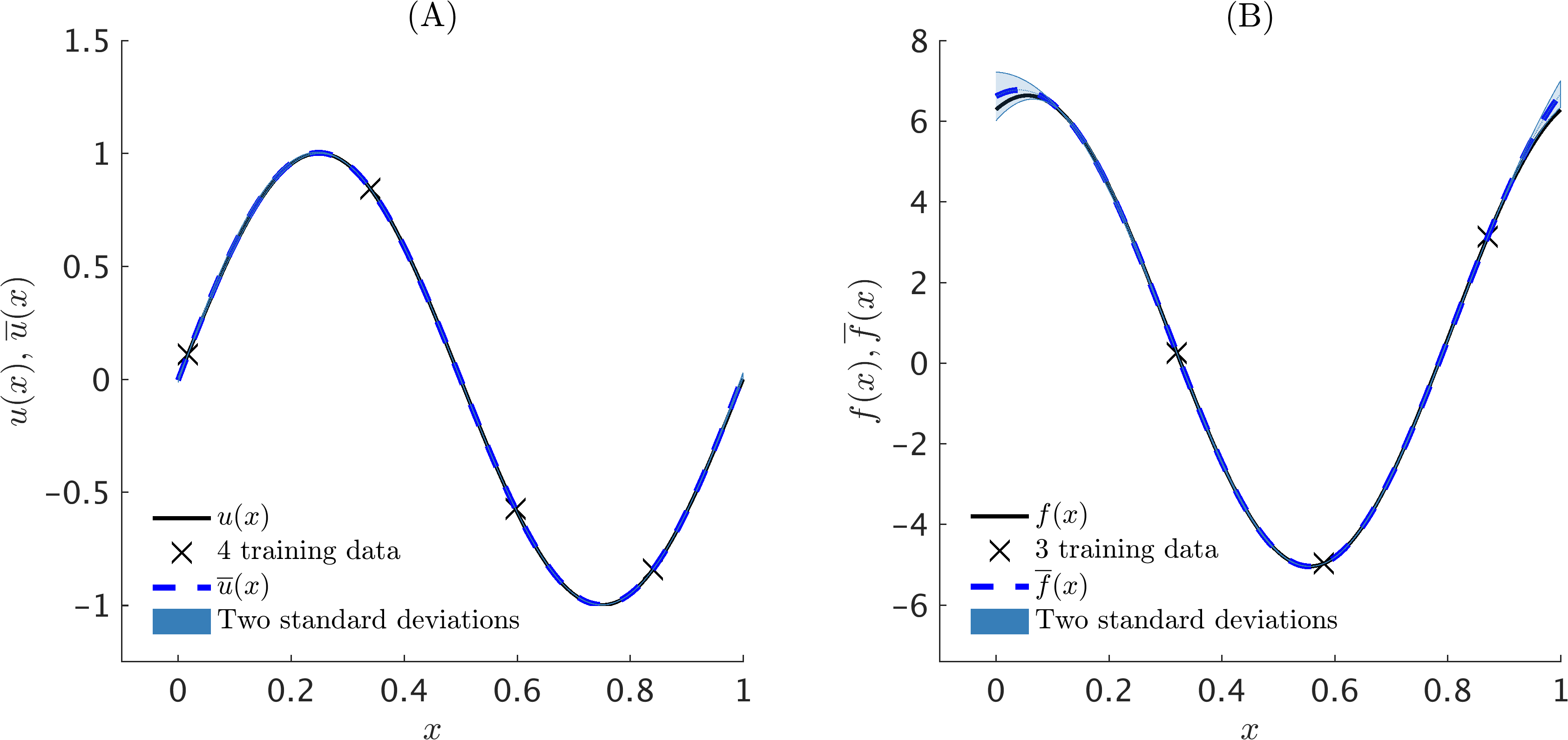
Note that for , the functions and satisfy this equation. In the following, the parameters will be infered from two types of data, namely, noise-free and noisy observations.
Noise-free data
Assume that the noise-free data , on , are generated according to , with , constituting of , data points chosen at random in the interval , respectively. Given these noise-free training data, the algorithm learns the parameters to have values . It should be emphasized that the algorithm is able to learn the parameters of the operator using only training data. Moreover, the resulting posterior distributions for and are depicted in Figure 1(A, B). The posterior variances could be used as good indicators of how uncertain one should be about the estimated parameters and predictions made based on these parameters.
Noisy data
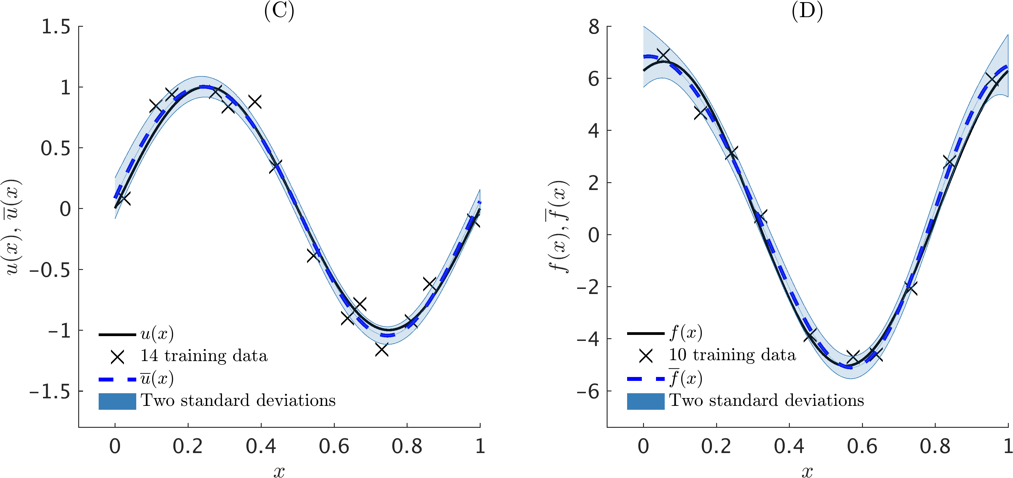
Consider the case where the noisy data , on , are generated according to , with , constituting of , data points chosen at random in the interval , respectively. Here, the noise and are randomly generated according to the normal distributions and , respectively. Given these noisy training data, the algorithm learns the parameters to have values . It should be emphasized that for this example the data is deliberately chosen to have a sizable noise. This highlights the ability of the method to handle highly noisy observations without any modifications. The resulting posterior distributions for and are depicted in Figure 1(C, D). The posterior variances not only quantify scarcity in observations but also signify noise levels in data.
3.2 Heat Equation
This example is chosen to highlight the capability of the proposed framework to handle time-dependent problems using only scattered space-time observations. To this end, consider the heat equation
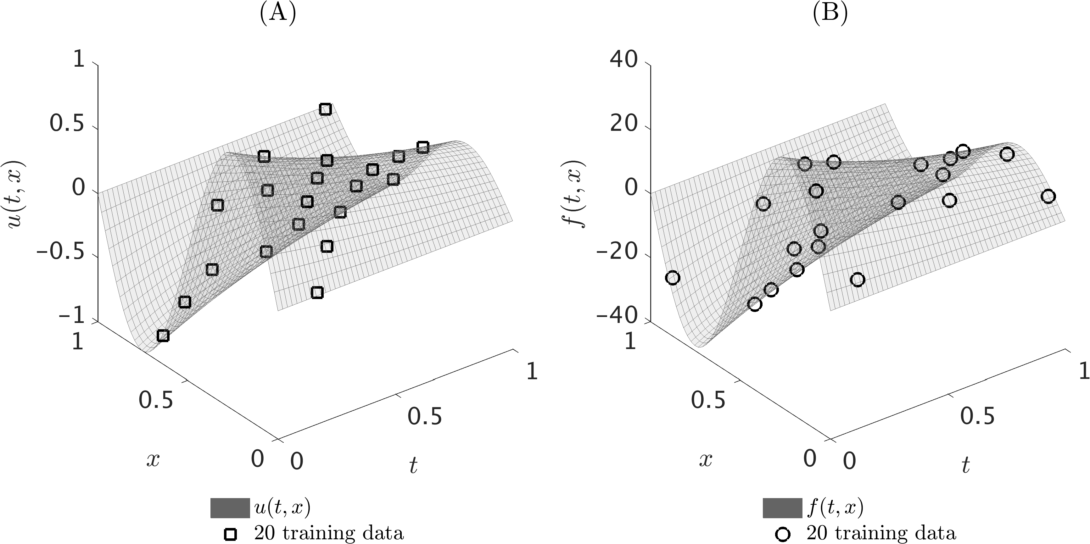
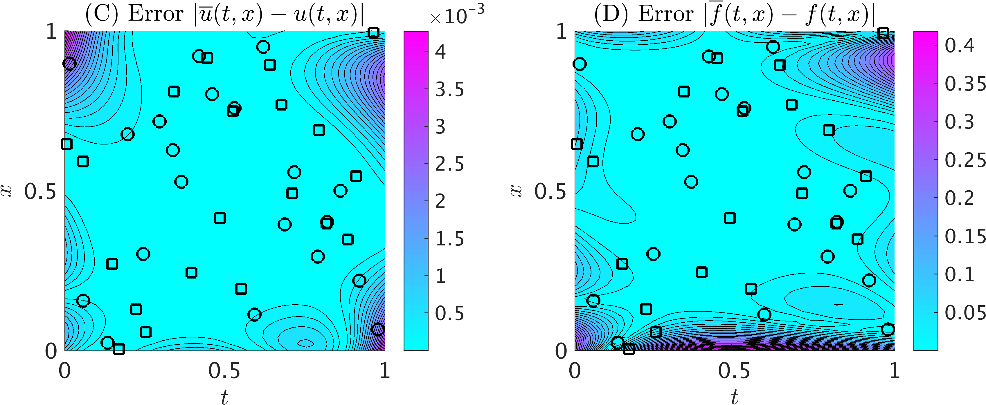
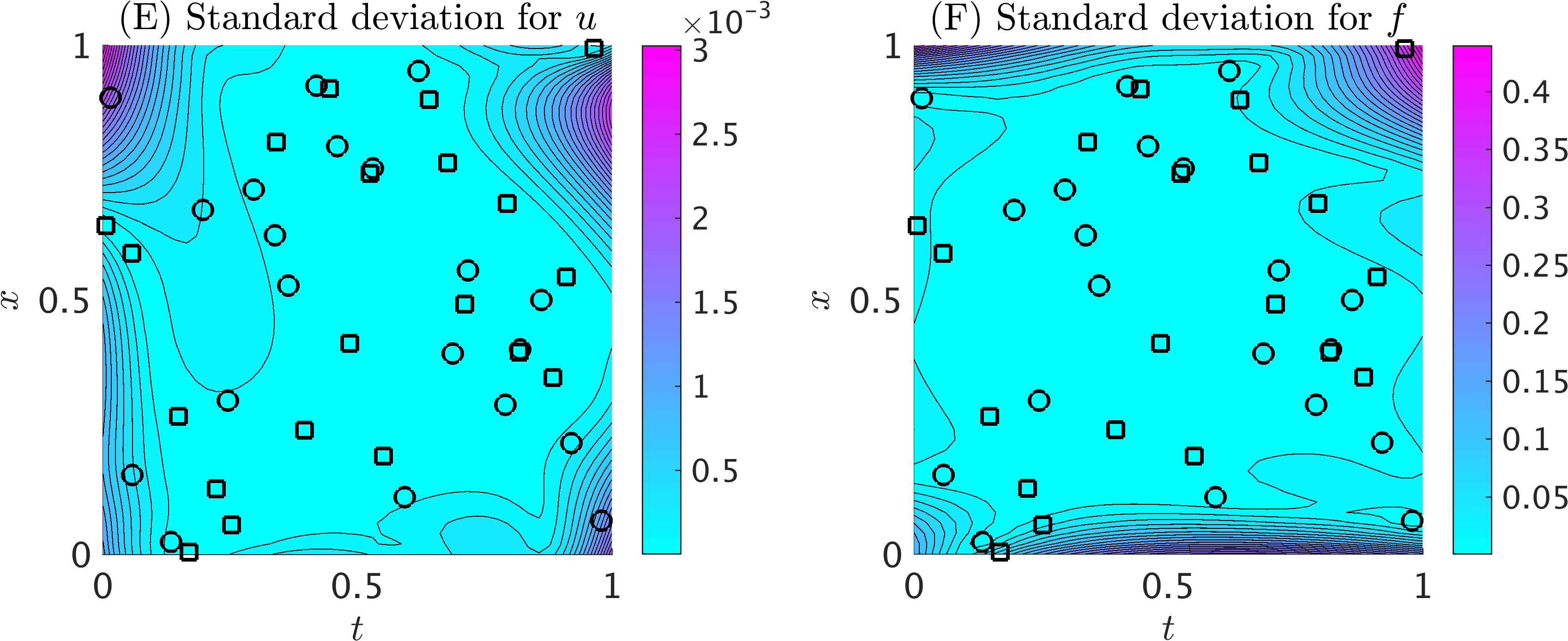
Note that for , the functions and satisfy this equation. Assume that the noise-free data , on , are generated according to , with , constituting of data points chosen at random in the domain , respectively. Given these training data, the algorithm learns the parameter to have value . The resulting posterior distributions for and are depicted in Figure 2. A visual inspection of this figure illustrates how closely uncertainty in predictions measured by posterior variances (see Figure 2(E, F)) correlate with prediction errors (see Figure 2(C, D)). Remarkably, the proposed methodology circumvents the need for temporal discretization, and is essentially immune to any restrictions arising due to time-stepping, e.g., the fundamental consistency and stability issues in classical numerical analysis.
3.3 Fractional Equation
Consider the one dimensional fractional equation
where is the fractional order of the operator that is defined in the Riemann-Liouville sense [37]. Fractional operators often arise in modeling anomalous diffusion processes. Their non-local behavior poses serious computational challenges as it involves costly convolution operations for resolving the underlying non-Markovian dynamics [37]. However, the machine leaning approach pursued in this work bypasses the need for numerical discretization, hence, overcomes these computational bottlenecks, and can seamlessly handle all such linear cases without any modifications. The only technicality induced by fractional operators has to do with deriving the kernel in Eq. 2. Here, was obtained by taking the inverse Fourier transform [37] of
where is the Fourier transform of the kernel . Similarly, one can obtain and .
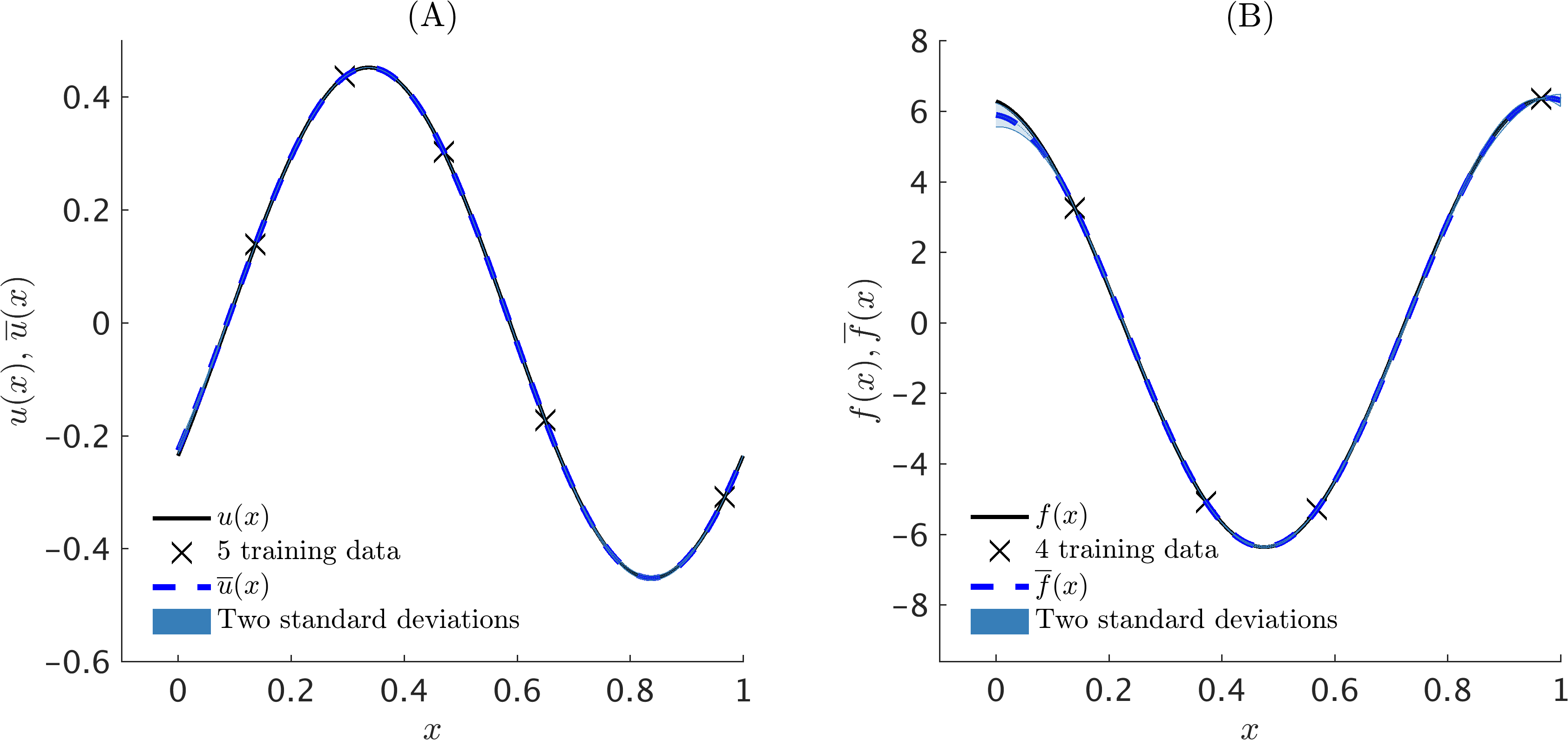
Note that for , the functions and satisfy the fractional equation. Assume that the noise-free data , on , are generated according to , with , constituting of , data points chosen at random in the interval , respectively. Given these noise-free training data, the algorithm learns the parameter to have value . The resulting posterior distributions for and are depicted in Figure 3.
3.4 Drosophila melanogaster gap gene dynamics [36, 16]
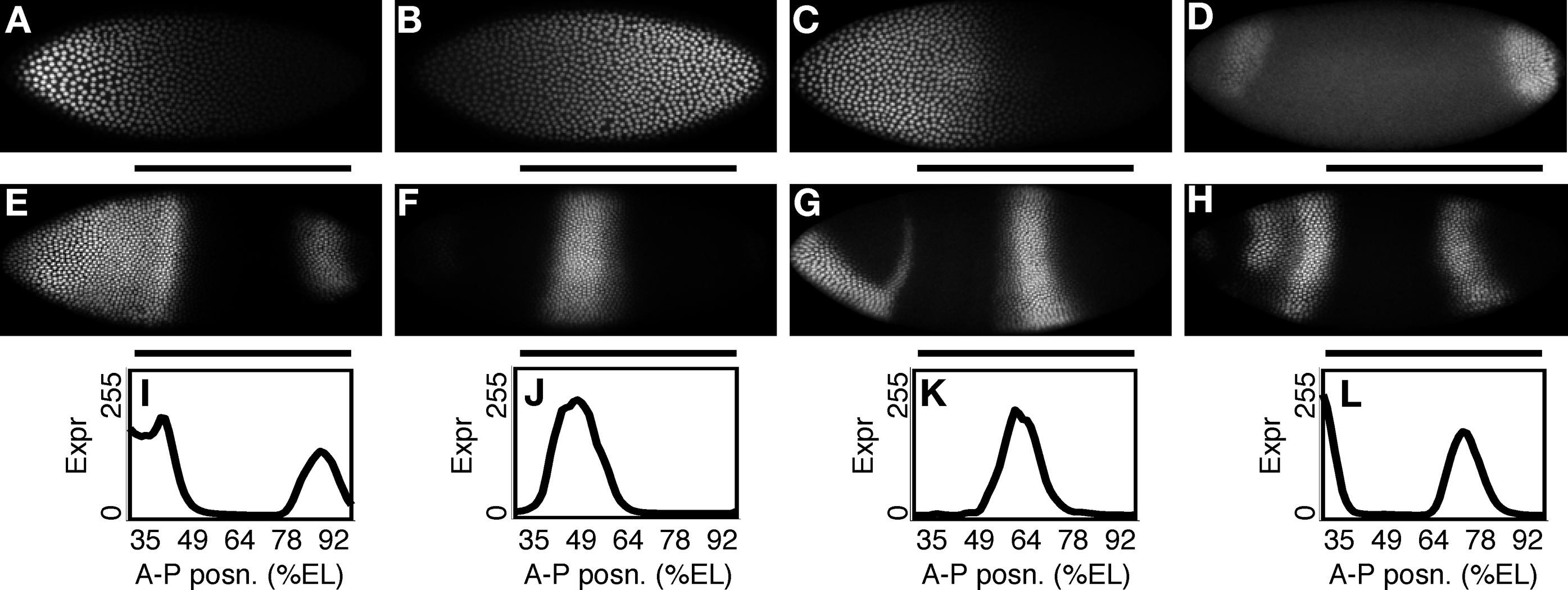
The gap gene dynamics of protein (see figure 4) can be modeled using a reaction-diffusion partial differential equation
where denotes the relative concentration of gap protein (unitless, ranging from 0 to 255) at space point (from 35% to 92% of embryo length) and time (0 min to 68 min after the start of cleavage cycle 13). Here, and are decay and diffusion rates of protein , respectively. Moreover, the right-hand-side is given by
where the term
models the doubling of nuclei and shutdown of transcription during mitosis and
specifies the production rate of protein . The model combines the processes of transcription and translation into a single production process . Here, is the maximum production rate,
and ranges over the seven genes (see figure 4). The regulatory weights , encode the effect protein has on the production rate of protein . If (or ), then gene is interpreted as being an activator (or a repressor) of gene .
| Max prod. | Regulatory weights () | Bias | |||||||
|---|---|---|---|---|---|---|---|---|---|
| Gene | rate () | Bcd | Cad | Hb | Kr | Gt | Kni | Tll | () |
| Hb | 32.03 | 0.1114 | -0.0054 | 0.0293 | -0.0124 | 0.0553 | -0.3903 | 0.0144 | -3.5 |
| Kr | 16.70 | 0.1173 | 0.0215 | -0.0498 | 0.0755 | -0.0141 | -0.0666 | -1.2036 | -3.5 |
| Gt | 25.15 | 0.0738 | 0.0180 | -0.0008 | -0.0758 | 0.0157 | 0.0056 | -0.0031 | -3.5 |
| Kni | 16.12 | 0.2146 | 0.0210 | -0.1891 | -0.0458 | -0.1458 | 0.0887 | -0.3028 | -3.5 |
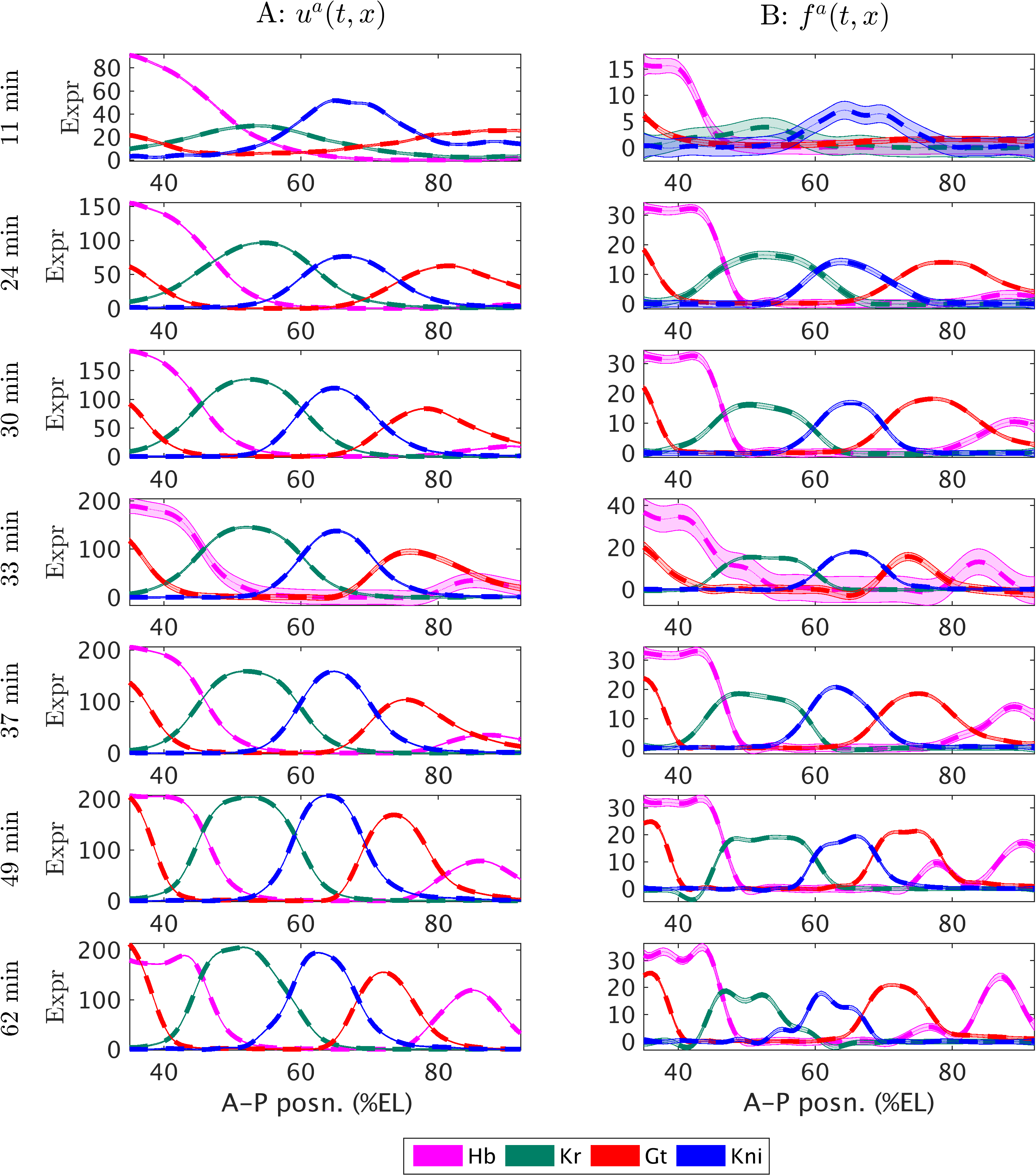
This work assumes the maximum production rate , the regulatory weights , and the bias or offset to be specified as in table 1 and seeks to learn the decay and diffusion rates of protein . In fact, table 2 summarizes the values learned by the algorithm for these parameters and figure 5 depicts the corresponding posterior distributions for and . Indeed, figure 5 gives a good indication of how certain one could be about the estimated parameters and the predictions made based on them.
| Decay | Diff. | |
|---|---|---|
| Gene | () | () |
| Hb | 0.1606 | 0.3669 |
| Kr | 0.0797 | 0.4490 |
| Gt | 0.1084 | 0.4543 |
| Kni | 0.0807 | 0.2683 |
4 Discussion
In summary, this work introduced a possibly disruptive probabilistic technology for learning general parametric linear equations from noisy data. This generality was demostrated using various bechmark problems with utterly different attributes along with an example application in functional genomics. Furthermore, the current methodology can be applied to inverse problems involving characterization of materials, tomography and electrophysiology, design of effective metamaterials, etc. The methodology can be straightforwardly generalized to address data with multiple levels of fidelity [24, 39] and equations with variable coefficients and complex geometries. Non-Gaussian and input-dependent noise models (e.g., student-t, heteroscedastic, etc.) [3] can also be accommodated. Moreover, systems of linear integro-differential equations can be addressed using multi-output Gaussian process regressions [40, 23, 22]. These scenarios are all feasible because they do not affect the key observation that any linear transformation of a Gaussian process is still a Gaussian process. In its current form, despite its generality regarding linear equations, the proposed framework cannot deal with non-linear equations. However, some specific non-linear operators can be addressed with extensions of the current framework by transforming such equations into systems of linear equations [41, 42] – albeit in high dimensions. In the end, the proposed methodology in this work, being essentially a regression technology, is suitable for resolving such high-dimensional problems.
References
- Kaipio and Somersalo [2006] J. Kaipio, E. Somersalo, Statistical and computational inverse problems, volume 160, Springer Science & Business Media, 2006.
- Stuart [2010] A. M. Stuart, Inverse problems: a bayesian perspective, Acta Numerica 19 (2010) 451–559.
- Williams and Rasmussen [2006] C. K. Williams, C. E. Rasmussen, Gaussian processes for machine learning, the MIT Press 2 (2006) 4.
- Murphy [2012] K. P. Murphy, Machine learning: a probabilistic perspective, MIT press, 2012.
- Diaconis [1988] P. Diaconis, Bayesian numerical analysis, Statistical decision theory and related topics IV 1 (1988) 163–175.
- Vapnik [2013] V. Vapnik, The nature of statistical learning theory, Springer Science & Business Media, 2013.
- Schölkopf and Smola [2002] B. Schölkopf, A. J. Smola, Learning with kernels: support vector machines, regularization, optimization, and beyond, MIT press, 2002.
- Tipping [2001] M. E. Tipping, Sparse bayesian learning and the relevance vector machine, The journal of machine learning research 1 (2001) 211–244.
- Tikhonov [1963] A. Tikhonov, Solution of incorrectly formulated problems and the regularization method, in: Soviet Math. Dokl., volume 5, pp. 1035–1038.
- Tikhonov and Arsenin [1977] A. N. Tikhonov, V. Y. Arsenin, Solutions of Ill-posed problems, W.H. Winston, 1977.
- Poggio and Girosi [1990] T. Poggio, F. Girosi, Networks for approximation and learning, Proceedings of the IEEE 78 (1990) 1481–1497.
- Franke and Schaback [1998] C. Franke, R. Schaback, Solving partial differential equations by collocation using radial basis functions, Applied Mathematics and Computation 93 (1998) 73–82.
- Fasshauer and Ye [2013] G. E. Fasshauer, Q. Ye, A kernel-based collocation method for elliptic partial differential equations with random coefficients, in: Monte Carlo and Quasi-Monte Carlo Methods 2012, Springer, 2013, pp. 331–347.
- Owhadi [2015] H. Owhadi, Bayesian numerical homogenization, Multiscale Modeling & Simulation 13 (2015) 812–828.
- Cockayne et al. [2016] J. Cockayne, C. Oates, T. Sullivan, M. Girolami, Probabilistic meshless methods for partial differential equations and bayesian inverse problems, arXiv preprint arXiv:1605.07811 (2016).
- Álvarez et al. [2013] M. A. Álvarez, D. Luengo, N. D. Lawrence, Linear latent force models using gaussian processes, IEEE transactions on pattern analysis and machine intelligence 35 (2013) 2693–2705.
- Alvarez et al. [2009] M. A. Alvarez, D. Luengo, N. D. Lawrence, Latent force models., in: AISTATS, volume 12, pp. 9–16.
- Lawrence [2005] N. Lawrence, Probabilistic non-linear principal component analysis with gaussian process latent variable models, Journal of Machine Learning Research 6 (2005) 1783–1816.
- Lawrence [2004] N. D. Lawrence, Gaussian process latent variable models for visualisation of high dimensional data, Advances in neural information processing systems 16 (2004) 329–336.
- Titsias and Lawrence [2010] M. K. Titsias, N. D. Lawrence, Bayesian gaussian process latent variable model., in: AISTATS, pp. 844–851.
- Higdon [2002] D. Higdon, Space and space-time modeling using process convolutions, in: Quantitative methods for current environmental issues, Springer, 2002, pp. 37–56.
- Boyle and Frean [2004] P. Boyle, M. Frean, Dependent gaussian processes, in: Advances in neural information processing systems, pp. 217–224.
- Alvarez and Lawrence [2009] M. Alvarez, N. D. Lawrence, Sparse convolved gaussian processes for multi-output regression, in: Advances in neural information processing systems, pp. 57–64.
- Kennedy and O’Hagan [2000] M. C. Kennedy, A. O’Hagan, Predicting the output from a complex computer code when fast approximations are available, Biometrika 87 (2000) 1–13.
- Le Gratiet and Garnier [2014] L. Le Gratiet, J. Garnier, Recursive co-kriging model for design of computer experiments with multiple levels of fidelity, International Journal for Uncertainty Quantification 4 (2014).
- Aronszajn [1950] N. Aronszajn, Theory of reproducing kernels, Transactions of the American mathematical society 68 (1950) 337–404.
- Saitoh [1988] S. Saitoh, Theory of reproducing kernels and its applications, volume 189, Longman, 1988.
- Berlinet and Thomas-Agnan [2011] A. Berlinet, C. Thomas-Agnan, Reproducing kernel Hilbert spaces in probability and statistics, Springer Science & Business Media, 2011.
- Liu and Nocedal [1989] D. C. Liu, J. Nocedal, On the limited memory bfgs method for large scale optimization, Mathematical programming 45 (1989) 503–528.
- Rasmussen and Ghahramani [2001] C. E. Rasmussen, Z. Ghahramani, Occam’s razor, Advances in neural information processing systems (2001) 294–300.
- Snelson and Ghahramani [2005] E. Snelson, Z. Ghahramani, Sparse gaussian processes using pseudo-inputs, in: Advances in neural information processing systems, pp. 1257–1264.
- Hensman et al. [2013] J. Hensman, N. Fusi, N. D. Lawrence, Gaussian processes for big data, arXiv preprint arXiv:1309.6835 (2013).
- Cohn et al. [1996] D. A. Cohn, Z. Ghahramani, M. I. Jordan, Active learning with statistical models, Journal of artificial intelligence research (1996).
- Krause and Guestrin [2007] A. Krause, C. Guestrin, Nonmyopic active learning of gaussian processes: an exploration-exploitation approach, in: Proceedings of the 24th international conference on Machine learning, ACM, pp. 449–456.
- MacKay [1992] D. J. MacKay, Information-based objective functions for active data selection, Neural computation 4 (1992) 590–604.
- Perkins et al. [2006] T. J. Perkins, J. Jaeger, J. Reinitz, L. Glass, Reverse engineering the gap gene network of drosophila melanogaster, PLoS Comput Biol 2 (2006) e51.
- Podlubny [1998] I. Podlubny, Fractional differential equations: an introduction to fractional derivatives, fractional differential equations, to methods of their solution and some of their applications, volume 198, Academic press, 1998.
- Poustelnikova et al. [2004] E. Poustelnikova, A. Pisarev, M. Blagov, M. Samsonova, J. Reinitz, A database for management of gene expression data in situ, Bioinformatics 20 (2004) 2212–2221.
- Le Gratiet [2013] L. Le Gratiet, Multi-fidelity Gaussian process regression for computer experiments, Ph.D. thesis, Université Paris-Diderot-Paris VII, 2013.
- Osborne et al. [2008] M. A. Osborne, S. J. Roberts, A. Rogers, S. D. Ramchurn, N. R. Jennings, Towards real-time information processing of sensor network data using computationally efficient multi-output gaussian processes, in: Proceedings of the 7th international conference on Information processing in sensor networks, IEEE Computer Society, pp. 109–120.
- Zwanzig [1960] R. Zwanzig, Ensemble method in the theory of irreversibility, The Journal of Chemical Physics 33 (1960) 1338–1341.
- Chorin et al. [2000] A. J. Chorin, O. H. Hald, R. Kupferman, Optimal prediction and the mori–zwanzig representation of irreversible processes, Proceedings of the National Academy of Sciences 97 (2000) 2968–2973.