Abstract

A numerical procedure and its MAPLE implementation capable of rigorously, albeit in a brute-force manner, proving specific strict one-variable inequalities in specific finite intervals is described. The procedure is useful, for instance, to affirm strict lower bounds of specific functions.

2010 Mathematics Subject Classification. 26.70, 26A48, 26A51

Keywords. Inequalities, monotonicity, numerical procedure, MAPLE procedure.

 

1 Introduction

Is there a good way to prove

$$\left(\frac{1-3x}{2}\right)\ln\left(\frac{1-3x}{2}\right)+2\left(\frac{1-24x}{5}\right)\ln\left(\frac{1-24x}{5}\right)>\,\,3\left(\frac{1-15x}{4}\right)\ln\left(\frac{1-15x}{4}\right)$$ (1)

for $x\in[0,0.04]$, or

$$-\frac{\ln^{3}(2)}{2^{s}}+\frac{\ln^{3}(3)}{3^{s}}-\frac{\ln^{3}(4)}{4^{s}}+\frac{\ln^{3}(5)}{2\cdot 5^{s}}>0$$ (2)

for $s\in[0,1]$?

Each is a strict inequality involving only one variable (no parameters) in a specific finite interval. Such inequalities are rarely of general interest. No one will present any of them as a lemma, much less as a theorem. Yet, often in the proof of some general result, the need for verifying an inequality like that pops up. For instance, (2) appears in [1] and (1) in the proof of the non-negativity of a class of sine polynomials in $[0,\pi]$.

Numerical computation and graphing provide evidence for the validity of such an inequality, but obviously not as rigorous proofs. Nevertheless, a simple principle makes it possible to use numerics to rigorously prove the inequality. I dub it the DIF technique.

Let $f(x)=g_{1}(x)-g_{2}(x)$ be the difference of two increasing (decreasing) functions in an interval $[\alpha,\beta]$. To prove that $f(x)>0$ in $[\alpha,\beta]$, it suffices to exhibit a sequence of points $\left\{\tau_{k}\right\}_{k=1}^{n}$ such that $$\alpha=\tau_{1}<\tau_{2}<\cdots<\tau_{n}=\beta$$ and $$g_{2}(\tau_{i+1})<g_{1}(\tau_{i}),\qquad\forall i=1,2,...,n-1.$$ (3) $$\big{(}\,g_{2}(\tau_{i})<g_{1}(\tau_{i+1})\,\big{)}\hskip 93.89409pt$$

The obvious proof is omitted. The requirement of having to verify the inequality for all $x\in[\alpha,\beta]$ reduces to checking (3) only for a finite number of values.

In applying the principle to (1), the increasing functions

$$g_{1}(x)=\left(\frac{1-3x}{2}\right)\ln\left(\frac{1-3x}{2}\right)+2\left(\frac{1-24x}{5}\right)\ln\left(\frac{1-24x}{5}\right)$$

and

$$g_{2}(x)=3\left(\frac{1-15x}{4}\right)\ln\left(\frac{1-15x}{4}\right)$$

and $\tau_{k}=\left\{0,\,\,0.009,\,\,0.014,\,\,0.022,\,\,0.03,\,\,004\right\}$ meet the requirement. The choice of $\tau_{k}$ is obviously not unique; $\displaystyle\left\{0.005k\right\}_{k=1}^{8}$ also works.

In checking the inequalities $g_{2}(\tau_{i+1})\leq g_{1}(\tau_{i})$, I merely use the values of the two sides, computed using some numerical computer software. For example, MAPLE 13 gives

$$g_{2}(0.04)=-0.8059612084...<-0.7882434741...=g_{1}(0.023).$$

Some may object to this step on the ground that computer numerics contain rounding errors, thus making it unreliable. In fact, modern numerical software is highly accurate with calculations involving well-known functions. As long as we keep ourselves within a reasonable scope of the accuracy of the software, we should be very safe. MAPLE, by default, does its calculations with an accuracy of 10 digits. As long as the numerical inequality holds within a 5 or 6 digit accuracy, it should be very reliable. In case of doubt, one can instruct MAPLE to use a higher number of digits to recheck the inequality. For the extremely skeptical, they can employ interval arithmetic (available, for instance, as a toolbox of MATLAB) to quench any remaining doubt.

The DIF technique is summarized as follows:

Steps to prove a desired inequality                   $f(x)>0,\quad x\in[\alpha,\beta]$. 1. Find two ${\color[rgb]{1,0,0}\nearrow}$ (${\color[rgb]{1,0,0}\searrow}$) functions such that   $f(x)=g_{1}(x)-g_{2}(x)$. 2. Find points:         ${\color[rgb]{1,0,0}\tau_{1}<\tau_{2}<\cdots<\tau_{n}}\hskip 24.18483pt$ such that (3) holds.

To establish inequality (2), one can use

$$g_{1}(s)=\frac{\ln^{3}(3)}{3^{s}}+\frac{\ln^{3}(4)}{4^{s}},\quad g_{2}(s)=\frac{\ln^{3}(2)}{2^{s}}+\frac{\ln^{3}(5)}{2\cdot 5^{s}},$$

which are obviously decreasing functions, and the uniformly spaced sequence

$$\tau_{k}:0,\,\,0.02,\,\,...\mbox{ (increment by 0.02)},\,\,1.$$

Alternatively, one can use

$$g_{1}(s)=-\frac{\ln^{3}(2)}{2^{s}}+\frac{\ln^{3}(3)}{3^{s}}\,,\qquad g_{2}(s)=\frac{\ln^{3}(4)}{4^{s}}-\frac{\ln^{3}(5)}{2\cdot 5^{s}}\,,$$

for which a much shorter sequence is sufficient:

$$\tau_{k}:\quad 0,\,\,0.4,\,\,0.65,\,\,0.8,\,\,0.9,\,\,1.$$

To complete the proof, one must fill in a necessary step, namely, to show that $g_{1}(s)$ and $g_{2}(s)$ are decreasing. To that end, we can try to show that

$$g_{1}^{\prime}(s)=\frac{\ln^{4}(2)}{2^{s}}-\frac{\ln^{4}(3)}{3^{s}}<0$$

(and the analog $g_{2}^{\prime}(s)<0$), for which the DIF technique is applicable.

Remark 1.

The procedure has its limitations. It cannot handle non-strict inequalities, when $f(x)=0$ at $x=\alpha$ or $\beta$ or some difficult-to-compute interior point. Sometimes it can serve as part of the proof, using another trick to take care of the non-strict inequality in a neighborhood of the critical point. A similar remark applies to inequalities in a non-compact interval such as $[0,\infty)$.

Remark 2.

If the inequality involves other variables, e.g. in the form of parameters, the procedure fails. Again, it may be possible to find a way around the difficulty with some tricks.

Remark 3.

What can we do if $g_{1}(x)$ and/or $g_{2}(x)$ are not monotone?

If their critical points are known, we can simply verify the inequality in each of the sub-intervals sub-divided by the critical points. To handle the general case, we can choose a sufficient large (positive or negative) $n$ so that $(x-\alpha+1)^{n}(g_{1}(x)-g_{2}(x))$ is a difference of two monotone functions. In particular, we can use this technique to verify if a given value is a strict lower/upper bound of a given function.

Remark 4.

In practice, Step 1 together with a decent graphing of the functions $g_{1}(s)$ and $g_{2}(s)$, especially if the software allows you to zoom into any sub-interval of $[\alpha,\beta]$, is sufficient to offer 99% confidence that the desired inequality is valid. The provision of the sequence $\tau_{k}$ is mainly for the purpose of allowing other people to double check the assertion, especially in cases when $g_{1}(s)$ and $g_{2}(s)$ are extremely close together.

Remark 5.

For special classes of functions, there are other more efficient numerical procedures. For example, the Sturm procedure is the best choice for studying algebraic and trigonometric polynomials. See [2]–[4] for details.

2 MAPLE Procedure for Determining/Verifying $\tau_{k}$

Finding or verifying $\tau_{k}$, though conceptually straightforward, is tedious if done manually. We present a simple MAPLE procedure that can help in this aspect.

Let us first describe the usage of the procedure. The procedure is written in the MAPLE programming language and the code lines are typed into a file, say called dif. I used MAPLE 13 for the experiments. Very likely, the same code works all for other versions.

Usage:

      FIRST FORMAT dif(g1,g2,[a,b],...) g1, g2 are expressions representing the functions $g_{1}$ and $g_{2}$. $a$ and $b$ are the endpoints of the interval. In this form, the procedure outputs a sequence of numbers $\tau_{k}$ satisfying (3). Additional options: long=1       Verbose output steps=N      Maximal number of $\tau_{k}$ (default: 100) digits=n    How many decimal points       SECOND FORMAT dif(g1,g2,[t1,...,tn]) Verifies if t1, ..., t1 satisfy (3)

In an interactive MAPLE session, commands can be entered either in Text or Math mode. Below, the command are shown in the Text mode because it is easier to typeset. The Math mode input and output are also shown.

While inside a MAPLE session, the procedure is loaded by using the command read(dif).

Newer versions of MAPLE do not require the semicolon at the end of the command if typed in the Math mode. Some older versions may need it.

Examples:

     read(dif);  g1 := ((1-3*x)/2)*ln((1-3*x)/2) + 2*((1-24*x)/5)*ln((1-24*x)/5);  g2 := 3*((1-15*x)/4)*ln((1-15*x)/4);  dif(g2, g1, [0, 0.04]);                   # FIRST FORMAT  dif(g1, g2, [0, 0.04]);  dif(g1, g2, [0, 0.04], long=1);     

In this first format, the third input argument $[0,0.04]$ is a list of two numbers, representing $[\alpha,\beta]$. The output is shown below:

The procedure is written to mandate that the first argument is the larger function. In case of an error, the procedure will complain as shown. The procedure could have been easily rewritten to automatically swap the functions in that situation. However, I believe that the error checking feature serves as a further insurance of the proper choice of g1 and g2.

In the long=1 version, the output is a matrix of five columns. The first column is a count, namely $k$, of the points $\tau_{k}$ given in the second column. If $g_{i}(x)$ are increasing, the third column is $g_{1}(\tau_{k})$ and the fourth column is $g_{2}(\tau_{k+1})$. If $g_{i}(x)$ are decreasing, they are $g_{1}(\tau_{k+1})$ and $g_{2}(\tau_{k})$ instead. In all cases, the values in the third column should be larger than that in the same row of the fourth column; the fifth column is the difference between these values.

The last three columns are listed as a visual check to make sure that the claimed inequalities (3) are valid within reasonable computational errors. For example, if the values are computed with 10 (the default in MAPLE) digit accuracy, then the differences between the values in the third and fourth columns (i.e. the value in the fifth column) should be at least $0.0001$. If this is not true, the procedure can be rerun with increased accuracy, for example, with the MAPLE command “Digits := 20”.

It is the user’s responsibility to make sure that g1 and g2 are either both increasing or both decreasing in $[a,b]$. The procedure does not have the intelligence to verify that premise rigorously. In case that assumption is not valid, the procedure may still output some (useless) answer.

To help a bit, the long=1 option will plot the graphs of g1 (red curve) and g2 (blue) to allow the user do a visual check.

If the monotonicity of $g_{i}(x)$ is not obvious, try the DIF technique on $g_{i}^{\prime}(x)$.

Comments

• The variable used in g1 and g2 can be arbitrary. It does not matter if you have used $x$ or $y$; or $s$. The procedure automatically detects it.

• If there is more than one variable present in g1 and g2 (perhaps due to typos), an error message will be printed. More complicated error checking is not available. It is the responsibility of the user.

• dif fails if it takes more than 100 steps without reaching the right endpoint $\beta$ of the interval. This can mean either the desired inequality is false or the difference between $g_{1}(x)$ and $g_{2}(x)$ so small that it actually requires more than 100 points of $\tau_{k}$. One can try to exclude the latter by using the steps=N option with a larger N.

Further Examples

By default, dif rounds each $\tau_{k}$ down to a number of decimal digits compatible with about one-hundredth of the length of the interval $[\alpha,\beta]$. This can be altered with the option digits=n. Using a higher n may generate a shorter $\tau_{k}$ sequence. The specification of n is only suggestive. dif may ignore it if necessary due to computational accuracy.

The next two examples show the second format of the procedure. The third input argument is a list of more than two numbers, which are interpreted as a sequence of $\tau_{k}$ to be verified.

     dif(g1, g2, [0, 0.04], digits=5);  dif(g1, g2, [0, 0.009, 0.019, 0.025, 0.034, 0.04])        # SECOND FORMAT  dif(g1, g2, [0, 0.009, 0.017, 0.025, 0.034, 0.04])     

The output is shown below.

When the supplied sequence $\tau_{k}$ does not satisfy (3), the procedure will balk at the first instance of violation and print “false”. Failure is also indicated by the fact that the last element of the last column of the displayed matrix is negative.

In case of success, the display is similar to the regular long=1 option, but without the graphs of $g_{i}(x)$. If graphs are desired, add long=1.

3 Explanation of the MAPLE Code

We briefly explain the code, assuming that the reader has rudimentary knowledge of MAPLE programming.

The entire code (with added comments) is repeated in the Appendix. The reader can use cut and paste to transfer that to a file, called “dif”, on the computer.

We break the code (minus the comments) up into small chunks. Line numbers are added for reference and are not part of the code; they should not be typed in the file. Blank lines have been added for aesthetic purposes and are optional.

 

   

   1  ffloor := (x,n) \rightarrow  subsop(2=-n, convert(floor(x*10^n), float)): 

   

 

The first non-comment line in the file defines a separate procedure ffloor which is used by dif, in line 27. It is a useful one to add to the regular MAPLE repertoire. MAPLE has a built-in command floor(x) to round a floating point number x down to the nearest integer, but there is no command to conveniently round x to the nearest float with a given number of decimal places. One can achieve the effect by using the command: floor(10^n*x)/10^n.

The resulting value is correct. However, it is aesthetically undesirable because, in most cases, it will be printed with some annoying trailing 0’s. Using ffloor fixes that.

The rest of the code is dif proper.

 

   

   2  dif := proc(g1,g2,A,\{long:=0,steps:=100,digits:=-100,relax:=99\}) 

   3    local aa, bb, ga, gb, f1, f2, tt, t1, cc, acc, tau, inc, var, ev; 

   

 

These two lines specify the procedure name dif, the mandatory arguments g1, g2, and A, the optional arguments, and the local variables.

 

   

   4    ev := (a,g) \rightarrow  evalf(subs(var=a,g)); 

   

 

The next line defines a procedure ev(a,g) to be used only internally within dif, essentially as a shorthand for a frequent construction. It takes an expression g and computes its numerical value when a float a is substituted into the variable contained in g.

 

   

   5    var := indets(evalf([g1,g2]), name); 

   6    if nops(var) > 1 then 

   7       error "Functions have more than one variable: ", var; 

   8    else 

   9       var := var[1]; 

  10    end if; 

   

 

In line 5, indets(...) returns a list of variables found in g1 and g2, and stores it in var. Here evalf is called before invoking indets, because the latter thinks $\pi$, such as in $\sin(2\pi x)$, as a variable instead of as a constant. If var has more than one element, then an error is thrown; otherwise, we change var to mean the sole variable it contains.

 

   

  11    aa := A[1]; bb := A[-1]; 

  12    ga := ev(aa,g1); gb := ev(aa,g2); 

  13    if ga < gb then error "Function 1 is smaller. Swap the functions." 

  14    end if; 

   

 

Here we compute ga​ = $g_{1}(\alpha)$ and gb​ = $g_{2}(\alpha)$ and make sure that the former is larger.

 

   

  15    gb := ev(bb,g2); 

  

  16    if ga < gb then f1 := g1; f2 := g2; inc := 1; 

  17    else f1 := -g2; f2 := -g1; inc := 0; 

  18    end if; 

   

 

Next we compute gb​ = $g_{1}(\beta)$, using it to decide whether $g_{i}(x)$ are increasing or decreasing; this information is stored in the flag inc. Then f1 and f2 are assigned the appropriate expression, to be used later to compute $\tau_{k}$.

 

   

  19    if nops(A) = 2 then 

           ... 

  44    else 

           ... 

  58    end if; 

  59    end proc: 

   

 

The rest of the code is divided into two separate cases: lines 20–42 when the user asks for $\tau_{k}$, and lines 44–56 when the user wants to verify if the supplied $\tau_{k}$ work. Line 59 is the last line of the procedure and also of the file.

 

   

  20       if digits > 0 then 

  21          acc := digits 

  22       else acc := 2-floor(log10(bb-aa)) 

  23       end if; 

   

 

These lines assign to acc the number of digits.

 

   

  24       tau := [aa]; 

  25       tt := aa; ga := ev(aa,f1); gb := ev(bb,f2); cc := 0; 

  

  26       for cc from 1 to steps while (ga < gb) do 

  27         t1 := min(ffloor((relax*fsolve(f2=ga,var=tt..bb)+tt)/ 

                   (relax+1),acc),bb); 

  28         if t1 \leq  tt then acc := acc+1; next; end if; 

  29         tt := t1; tau := [op(tau),tt]; 

  30         ga := ev(tt,f1); 

  31       end do; 

   

 

The above is the loop to compute $\tau_{k}$. Ideally, if numerical computation were exact (and all inequalities were replaced by equality), then $\tau_{k}$ would have been determined recursively by: $\displaystyle\tau_{k}=g_{2}^{-1}(g_{1}(\tau_{k-1})).$ Geometrically, $\tau_{k}$ is the successive values of the iterative algorithm depicted in Figure 1.

Figure 1: Iterative determination of $\tau_{k}$.

$\tau_{2}$

$\tau_{3}$

$\tau_{4}$

$\tau_{5}$

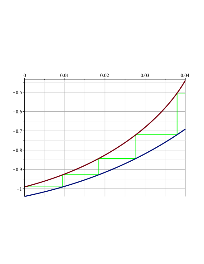
In practice, we have to make $\tau_{k}$ smaller; this is done in line 27 using relax. By default relax=99, and that can be altered by the user. Choosing a smaller relax makes $\tau_{k}$ smaller.

The variable cc counts the number of iterations. The loop exits either if cc exceeds the assigned number of steps or if $\tau_{k}$ has reached the right endpoint $\beta$ of the interval.

 

   

  32       if ga < gb then 

  33          cc := min(steps,5); 

  34          printf("    **** Fails after %d steps. Last %d steps are: ", 

                 steps, cc); 

  35          print(tau[-cc..-1]); 

   

 

In the former case, a failure message is displayed.

 

   

  36       else 

  37          tau := [op(tau),bb]; 

  38          if long = 1 then 

  39             dif(g1,g2,tau); 

  40             plot([g1,g2],var=aa..bb,gridlines=true,size=[550,400]); 

  41          else tau; 

  43          end if; 

  44       end if; 

   

 

Otherwise, line 36 adds $\beta$ as the last $\tau_{k}$. If the long=1 option is set, dif is invoked with the second format to print the verbose output, and the graphs of $g_{i}(x)$ are plotted. Without the verbose option, only the sequence tau is displayed.

 

   

  45       t1 := nops(A); 

  46       for cc from 1 to t1-1 do 

  47          ga := ev(A[cc+1-inc],g1); gb := ev(A[cc+inc],g2); 

  48          if cc = 1 then 

  49             tau := <1 | A[1] | ga | gb | ga-gb >; 

  50          else 

  51             tau := <tau,<cc | A[cc] | ga | gb | ga-gb >>; 

  52          end if; 

  53          if ga < gb then print(tau); return false; end if; 

  54       end do; 

  55       ga := ev(A[-1],g1); gb := ev(A[-1],g2); 

  56       tau := <tau,<t1 | A[-1] | ga | gb | ga-gb >>; 

  57       print(tau); 

   

 

This final part of the code handles the long display when dif is invoked in the second format, with supplied $\tau_{k}$. In this format, $\tau_{k}$ is given in the input variable A. The variable tau, on the other hand, is free to be used for another purpose, namely, to store the matrix containing the five columns of numbers to be displayed at the end. Lines 45–53 is the loop to build the rows (except the last one which is filled in by line 55) of the matrix. Line 53 prints the partial tau and returns “false” in case condition (3) fails. Line 56 prints the matrix and the job is done.

Appendix: The Entire MAPLE Code

# CUT AND PAST THE FOLLOWING LINES INTO A FILE CALLED "dif"

#  ffloor(x,n)         ROUND FLOAT x DOWN TO n DECIMAL PLACES
ffloor := (x,n) -> subsop(2=-n, convert(floor(x*10^n), float)):

#  dif(g1,g2,A,...)    SEE SECTION ON USAGE
dif := proc(g1,g2,A,{long:=0,steps:=100,digits:=-100,relax:=99})
  local aa, bb, ga, gb, f1, f2, tt, t1, cc, acc, tau, inc, var, ev;

  #  ev(a,g)           EVALUATE g TO FLOAT, SUBSTITUTING var=a
  ev := (a,g) -> evalf(subs(var=a,g));

  # DETERMINES THE VARIABLE IN g
  var := indets(evalf([g1,g2]), name);
  if nops(var) > 1 then
     error "Functions have more than one variable: ", var;
  else
     var := var[1];
  end if;

  # CHECK IF g1 > g2
  aa := A[1]; bb := A[-1];
  ga := ev(aa,g1); gb := ev(aa,g2);
  if ga < gb then error "Function 1 is smaller. Swap the functions."
  end if;

  # DETERMINE IF g1 IS INCREASING OR DECREASING
  gb := ev(bb,g1);
  if ga < gb then f1 := g1; f2 := g2; inc := 1;
  else f1 := -g2; f2 := -g1; inc := 0;
  end if;

  if nops(A) = 2 then

     # FIRST FORMAT OF INVOCATION: DETERMINE [ tau_k ]
     if digits > 0 then
        acc := digits
     else acc := 2-floor(log10(bb-aa))
     end if;
     tau := [aa];
     tt := aa; ga := ev(aa,f1); gb := ev(bb,f2); cc := 0;

     # LOOP TO DETERMINE tau_k
     for cc from 1 to steps while (ga < gb) do
       t1 := min(ffloor((relax*fsolve(f2=ga,var=tt..bb)+tt)/(relax+1),acc),bb);
       if t1 <= tt then acc := acc+1; next; end if;
       tt := t1; tau := [op(tau),tt];
       ga := ev(tt,f1);
     end do;

     if ga < gb then
        # FAIL
        cc := min(steps,5);
        printf("    **** Fails after %d steps. Last %d steps are: ", steps, cc);
        print(tau[-cc..-1]);
     else
        # SUCCESS
        tau := [op(tau),bb];
        if long = 1 then
           dif(g1,g2,tau);
           plot([g1,g2],var=aa..bb,gridlines=true,size=[550,400]);
        else tau;
        end if;
     end if;

  else

     # SECOND FORMAT OF INVOCATION: VERIFY [ tau_k ]
     t1 := nops(A);

     # BUILD MATRIX tau
     for cc from 1 to t1-1 do
        ga := ev(A[cc+1-inc],g1); gb := ev(A[cc+inc],g2);
        if cc = 1 then
           tau := <1 | A[1] | ga | gb | ga-gb >;
        else
           tau := <tau,<cc | A[cc] | ga | gb | ga-gb >>;
        end if;
        if ga < gb then print(tau); return false; end if;
     end do;

     ga := ev(A[-1],g1); gb := ev(A[-1],g2);
     tau := <tau,<t1 | A[-1] | ga | gb | ga-gb >>;

     print(tau);
  end if;
  end proc:                         # END OF FILE

References

- [1] H. Alzer and M.K. Kwong, On the concavity of Dirichlet’s eta function and related functional inequalities, Journal of Number Theory 151 (2015), 172-196.
- [2] H. Alzer and M.K. Kwong, Sturm’s theorem and a refinement of Vietoris’ inequality for cosine polynomials, arXiv:1406.0689 (math.CA).
- [3] Nonnegative trigonometric polynomials and Sturm’s theorem, arXiv:1507.00494 [math.CA] (2015).
- [4] Nonnegative trigonometric polynomials, Sturm’s theorem, and symbolic computation, arXiv:1402.6778 [math.CA] (2014).