Analysis and design of Raptor codes using a multi-edge framework

Abstract

The focus of this paper is on the analysis and design of Raptor codes using a multi-edge framework. In this regard, we first represent the Raptor code as a multi-edge type low-density parity-check (MET-LDPC) code. This MET representation gives a general framework to analyze and design Raptor codes over a binary input additive white Gaussian noise channel using MET density evolution (MET-DE). We consider a joint decoding scheme based on the belief propagation (BP) decoding for Raptor codes in the multi-edge framework, and analyze the convergence behavior of the BP decoder using MET-DE. In joint decoding of Raptor codes, the component codes correspond to inner code and precode are decoded in parallel and provide information to each other. We also derive an exact expression for the stability of Raptor codes with joint decoding. We then propose an efficient Raptor code design method using the multi-edge framework, where we simultaneously optimize the inner code and the precode. Finally we consider performance–complexity trade–offs of Raptor codes using the multi-edge framework. Through density evolution analysis we show that the designed Raptor codes using the multi-edge framework outperform the existing Raptor codes in literature in terms of the realized rate.

I Introduction

The introduction of graph-based codes together with the belief propagation (BP) decoding [1], has made a significant change in the field of error correcting codes in terms of low-complexity decoding. Generally, a graph-based code can be represented by a Tanner graph in which variable and check nodes respectively correspond to the codeword symbols and the parity check constraints [2]. One of the most prominent classes of graph-based codes for which the BP decoding algorithm gives near-capacity performance is low-density parity-check (LDPC) codes invented by Gallager [3]. As a unifying framework for graph-based codes, Richardson and Urbanke [4] introduced multi-edge type low-density parity-check (MET-LDPC) codes to control the Tanner graph structure of random code ensembles. A code ensemble is the set of all possible codes with a particular degree distribution of their Tanner graph representation.

A numerical technique, called MET density evolution (MET-DE) [5] has been widely used for analysis and design of MET-LDPC code ensembles under BP decoding. MET-DE determines the asymptotic behavior of the BP decoding for a given MET-LDPC code ensemble by iteratively tracking the probability density function (PDF) of messages passed along the edges in the corresponding Tanner graph. Applying MET-DE to a given MET-LDPC code ensemble, one can predict how codes (with a large enough code length) from that ensemble behave on average. MET-DE allows finding the optimal degree distribution independent of the choice of code length or Tanner graph structure, which is the first step in any design or analysis of MET-LDPC codes.

Fountain codes [6] are a class of graph-based codes, which have been inspired by the idea of rateless coding, originally proposed for data transmission over erasure channels. Luby Transform (LT) codes [7] are the first class of efficient Fountain codes, which are essentially a type of low-density generator matrix (LDGM) codes [8] with an average input bit degree that grows logarithmically. This logarithmic growth causes several problems, such as increased complexity of encoder and decoder, and also results in large error floors. Raptor codes [9] are an extension of LT codes that overcome these problems. A Raptor code is a simple concatenation of an inner LT code with an outer code, called precode, which is usually a high rate LDPC code.

Although the Raptor code design has been well investigated for different binary channels [9, 10, 11, 12, 13, 14, 15, 16], there has been little progress on universal design methods for the binary-input additive white Gaussian noise (BI-AWGN) channel, and a complete analysis of the asymptotic performance of Raptor codes is still missing. Performance of Raptor codes over the BI-AWGN channel has been investigated in [12, 13], and shown that the realized rate of a well-designed Raptor code can approach the capacity bound. Shirvanimoghaddam et al. [10] studied the design of Raptor codes over BI-AWGN channels in the low signal-to-noise ratio (SNR) regime and showed that properly designed Raptor codes can achieve rate efficiency larger than 0.95 in that regime. Pakzad et al. [17] studied different design principles, such as code length and complexity of the decoding, for finite-length Raptor codes under BP decoding for BI-AWGN channels. However, all these methods only considered the performance of the LT code component of the Raptor code for a given precode. A high-rate regular LDPC code [14, 15] or a high-rate LDPC code with left-regular and right Poisson distributed parity check matrix [12, 13] has been widely used for the precode of Raptor codes in order to minimize the rate loss due to the precoding. This motivates us to propose a more general design framework for Raptor codes using a multi-edge framework. The multi-edge framework enables us to perform a comprehensive analysis of the asymptotic performance of the entire Raptor code including both the LT code and the LDPC code.

All the design methods proposed in literature on Raptor codes over BI-AWGN channel have relied on linear programming based on approximate DE algorithms namely, the extrinsic information transfer (EXIT) chart analysis [18, 13] or Gaussian approximation [19]. These approximate DE algorithms are based on the assumption of symmetric Gaussian distribution for the DE messages. However, this assumption may not be accurate [20], particularly at low rates and with punctured variable nodes, which is the case for Raptor codes. Therefore, the approximate DE algorithms can negatively impact the search for optimal code ensembles.

The decoding process for Raptor codes generally consists of a series of decoding attempts, which progressively collects LT coded symbols until the decoder is confident that the transmitted message is correctly decoded. Basically a Raptor decoding attempt consists of two decoding processes: the LT decoding process and the LDPC decoding process (collectively know as Raptor decoding process). Each of these decoding processes runs a predetermined number of BP decoding iterations in which the soft information is passed back and forth along the edges in the corresponding Tanner graph. The way that the soft information is exchanging between two decoding processes depends on the configuration of the Raptor decoder (i.e., tandem decoding or joint decoding). The conventional design strategy of Raptor codes is mainly based on tandem decoding, where the LT component is decoded first and soft information is then send to the precoder. Venkian et al. [14] however showed that tandem decoding is sub-optimal compared to joint decoding, where both component codes are decoded in parallel and extrinsic information (i.e., the information from previous BP decoding iteration) is exchanged between the decoders. Unfortunately, only few studies [14] have considered joint decoding of Raptor codes. Further, there is no design strategy for the joint design of component codes of Raptor codes, using joint or tandem decoding.

Moreover, the traditional tandem decoding scheme proposed for Raptor codes starts the LT decoding process from scratch at every decoding attempt, without using soft information produced in the previous decoding attempt. We refer to this decoding strategy as message-reset decoding. Another possible decoding strategy for the LT decoding process in the tandem decoding scheme is to reuse the soft information produced in the previous decoding attempt. We refer to this decoding strategy as incremental decoding. To-date only few results [11] are available concerning the performance and the decoding complexity trade-off for Raptor codes over the BI-AWGN channel.

I-A Main contribution

The main contributions of this paper are as follows:

1. We study Raptor codes using the multi-edge framework, where we represent the Raptor code as a MET-LDPC code, which is the serial concatenation of an LT code and an LDPC code (i.e., precode). This MET representation gives us a more unifying framework to analyze and design Raptor codes with the help of analytical tools used for MET-LDPC code, such as MET-DE [4].

2. We consider two decoding schemes for Raptor codes under the multi-edge framework, including tandem and joint decoding. We derive the stability conditions under tandem decoding using the multi-edge framework and re-derive the existing stability conditions from [12]. We then derive an exact expression for the stability of Raptor codes under joint decoding using the multi-edge framework. We analyze Raptor codes using both tandem and joint decoding, and show the benefits of joint decoding.

3. We then propose a joint Raptor code design method by including degree distributions of both LT and LDPC code components as variables in the optimization. This provides a framework for a better selection of the LDPC code component depending on the channel SNR for which the code is designed (designed SNR) and the degree distributions of the LT code component. We formulate the optimization problem for Raptor codes for a given channel SNR as a non-liner cost function maximization problem, where the realized rate (which is computed from MET-DE) is the cost function and the degree distributions of LT and LDPC code components give the variables to be optimized. The realized rate of a Raptor code is defined as the ratio of the length of the information vector, and the average number of Raptor coded symbols required for the successful decoding at the destination. Moreover, our optimization method is based on the MET-DE, which in turn helps to increase the accuracy of the final result in the code optimization. Because we are no longer use any approximate DE algorithms such as EXIT charts and Gaussian approximation, which are previously used to optimize Raptor codes. Through MET-DE, we show that designed and/or evaluated Raptor codes using joint decoding always give better rate efficiency results than the one with tandem decoding. This seems to be significant when the evaluated SNR is below the designed SNR.

4. Finally, we implement a tandem decoding scheme based on the incremental decoding strategy using the multi-edge framework, propose a modification to reduce complexity and show the advantage of considering the incremental decoding strategy in the design of the Raptor codes.

I-B Organization

The rest of the paper is organized as follows. Section II presents a representation of Raptor codes in the multi-edge framework. In Section III, we describe two possible decoding schemes based on the BP decoding for Raptor codes using MET-DE. Section IV provides the design methods of Raptor codes in the multi-edge framework. Analytical results are shown in Section V. Finally, Section VI concludes the paper.

II Representation of Raptor codes in the multi-edge framework

In this section, we describe the new representation of Raptor codes as MET-LDPC codes. A Raptor code specified by parameters $(k,\mathcal{C},\Omega(x))$ is a serial concatenation of an inner LT code with degree distribution $\Omega(x)$, and a precode $\mathcal{C}$, generally a high-rate LDPC code. For a Raptor code, first, the $k$ bit information vector is precoded using a rate $\mathcal{R}_{\mathrm{LDPC}}=k/n$ LDPC code to generate $n$ LDPC coded symbols, referred to as input bits. Then using an LT code with degree distribution $\Omega(x)$, a potentially limitless number of LT coded symbols, referred to as output bits, are generated. Each output bit is the XOR of $d$ randomly selected input bits, where $d$ is randomly obtained from $\Omega(x)$. The realized rate of the LT code is $\mathcal{R}_{\mathrm{LT}}=n/\hat{m}$, where $\hat{m}$ is the average number of LT coded symbols required for a successful decoding. An example Tanner graph of a Raptor code truncated at code length $m$ is shown in Fig. 1(a).

(a) An example Tanner graph of a Raptor code with parameters $(k,\mathcal{C},\Omega(x))$ truncated at code length $m$, where $p_{i}$ represents the fraction of degree $i$ nodes.

(b) Graphical representation of a Raptor code ensemble as a MET-LDPC code ensemble, where ‘$\Circle$’, ‘$\CIRCLE$’, and ‘$\Square$’  respectively represent unpunctured variable nodes, punctured variable nodes and check nodes, and ‘$\Pi_{i}$’  represents the edge-type $i$. The number of nodes for different edge-types (i.e., $L_{[\dots]}$ and $R_{[\dots]}$) are defined as fractions of $m$. Note that $k_{v}=k_{c}=1$.

Figure 1: Graphical representation of a Raptor code.

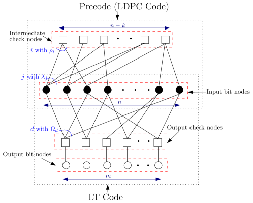
Using the multi-edge framework, the Tanner graph of a Raptor code ensemble can be drawn as shown in Fig. 1(b). This graph has three edge-types, where edge-type $\Pi_{1}$ represents the precode $\mathcal{C}$ and edge-type $\Pi_{2}$ represents the LT code with degree distribution $\Omega(x)$. Edge-type $\Pi_{3}$ is used to include the output bits which transfer channel information to the LT code. Moreover, the sub-graph comprising with edge-types $\Pi_{2}$ and $\Pi_{3}$ can be considered as an LDGM code.

The Raptor code ensemble in the multi-edge framework can be represented by two node-perspective multinomials associated with variable nodes and check nodes as follows:

$$L(\boldsymbol{r},\boldsymbol{x}) =r_{0}~{}\sum_{i_{v}=1}^{i_{v_{\max}}}~{}\sum_{j_{v}=1}^{{j_{v_{\max}}}}L_{[i_{v}~{}j_{v}~{}0]}~{}x_{1}^{i_{v}}~{}x_{2}^{j_{v}}~{}+~{}r_{1}~{}L_{[0~{}0~{}1]}~{}x_{3},$$ (1)

$$R(\boldsymbol{x}) =\sum_{i_{c}=2}^{{i_{c_{\max}}}}R_{[i_{c}~{}0~{}0]}~{}x_{1}^{i_{c}}~{}+~{}\sum_{j_{v}=1}^{{j_{c_{\max}}}}R_{[0~{}j_{c}~{}1]}~{}x_{2}^{j_{c}}~{}x_{3},$$ (2)

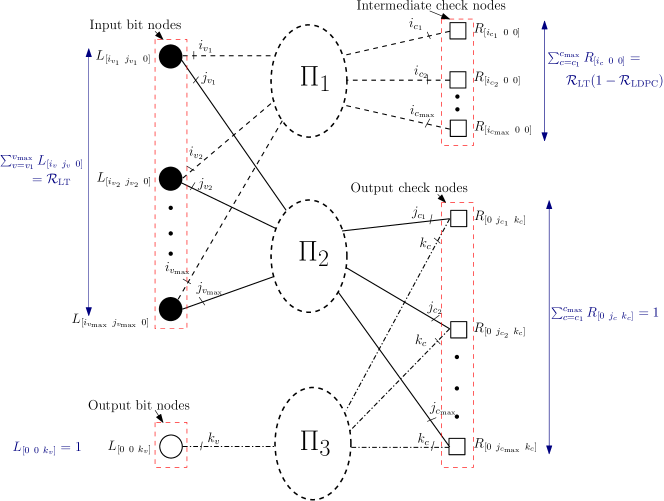
where $\boldsymbol{x}$ and $\boldsymbol{r}$ are vectors defined as follows. The vector $\boldsymbol{x}=[x_{1},x_{2},x_{3}]$ corresponds to each edge-type in the Tanner graph and $x_{p}^{k}$ is used to indicate the number of edges of the $p$th edge-type connected to a particular node. The vector $\boldsymbol{r}=[r_{0},r_{1}]$ associated with each variable node, corresponds to the channel to which the variable node is connected. In the multi-edge framework, the input bits are considered as punctured variable nodes (i.e., which are not transmitting over the channel) and denoted by $r_{0}$. The output bits are considered as unpunctured variable nodes (i.e., which are transmitting over a single channel) and denoted by $r_{1}$. Finally, we use $[i~{}j~{}k]$ to categorize the node types, where $i,j$ and $k$, respectively denote the number of edges of the edge-type 1, 2 and 3 connected to that node, i.e., $L_{[i_{v}~{}j_{v}~{}k_{v}]}$ and $R_{[i_{c}~{}j_{c}~{}k_{c}]}$ correspond to the fraction of variable nodes of type ${[i_{v}~{}j_{v}~{}k_{v}]}$ and the fraction of check nodes of type ${[i_{c}~{}j_{c}~{}k_{c}]}$, where the fractions are relative to the number of transmitted variable nodes.

In order to impose the Raptor code structure in the MET-LDPC framework, we add some additional constraints into (1) and (2).

$$L_{[0~{}0~{}1]} =1,$$ (3)

$$\sum_{j_{c}=1}^{{j_{c_{\max}}}}R_{[0~{}j_{c}~{}1]} =1,$$ (4)

$$\sum_{i_{v}=2}^{i_{v_{\max}}}~{}\sum_{j_{v}=1}^{j_{v_{\max}}}L_{[i_{v}~{}j_{v}~{}0]} =\mathcal{R}_{\mathrm{LT}},$$ (5)

$$\sum_{i_{c}=1}^{{i_{c_{\max}}}}R_{[i_{c}~{}0~{}0]} =\mathcal{R}_{\mathrm{LT}}(1-\mathcal{R}_{\mathrm{LDPC}}).$$ (6)

Constraints (3) and (4) are used to satisfy the constraints on the total number of transmitted bits as fractions of code length. Constraints (5) and (6) are used to compute the rates of LT and LDPC code components in multi-edge framework. The realized rate of the Raptor code for a given SNR, $\gamma$, in the multi-edge framework can be computed as [5, page 383]

$$\mathcal{R}(\gamma) =L(\boldsymbol{1},\boldsymbol{1})-R(\boldsymbol{1}),$$ (7)

where $\boldsymbol{1}$ denotes a vector of all $1$’s with the length determined by the context. The rate efficiency of the Raptor code is then computed as

$$\eta(\gamma) =\frac{\mathcal{R}(\gamma)}{C(\gamma)},$$ (8)

where $C(\gamma)$ is the capacity of the BI-AWGN channel at SNR, $\gamma$, which is given by [12]

$$C(\gamma) =1-\frac{1}{\sqrt{8\pi\gamma}}\int_{-\infty}^{\infty}\log_{2}\left(1+e^{-x}\right)e^{-\frac{(x-2\gamma)^{2}}{8\gamma}}dx.$$ (9)

Finally, we specify the standard notation of the Raptor code with parameter $(k,\mathcal{C},\Omega(x))$ using the MET notation as follows. The node-perspective degree distribution related with LT code, $\Omega(x)$, can be computed from (2) as follows:

$$\Omega(x) =\sum_{j_{c}=1}^{j_{c_{\max}}}R_{[0~{}j_{c}~{}1]}~{}x^{j_{c}},$$ (10)

where $R_{[0~{}j_{c}~{}1]}$ denotes the fraction of output bits with degree $j_{c}$, which is $\Omega_{j_{c}}$. The edge-perspective degree distributions associated with variable nodes and check nodes of the precode ($\lambda(\boldsymbol{x})$ and $\rho(\boldsymbol{x})$) can be computed from (1) and (2) as follows:

$$\lambda(\boldsymbol{x}) =\frac{L_{x_{1}}(\boldsymbol{r},\boldsymbol{x})}{L_{x_{1}}(\boldsymbol{1},\boldsymbol{1})}\hskip 28.45274pt\text{and}\hskip 28.45274pt\rho(\boldsymbol{x})=\frac{R_{x_{1}}(\boldsymbol{x})}{R_{x_{1}}(\boldsymbol{1})},$$ (11)

where $L_{x_{1}}(\boldsymbol{r},\boldsymbol{x})=\frac{dL(\boldsymbol{r},\boldsymbol{x})}{d{x_{1}}}$ and $R_{x_{1}}(\boldsymbol{x})=\frac{dR(\boldsymbol{x})}{d{x_{1}}}$.

III Decoding of Raptor codes in the multi-edge framework

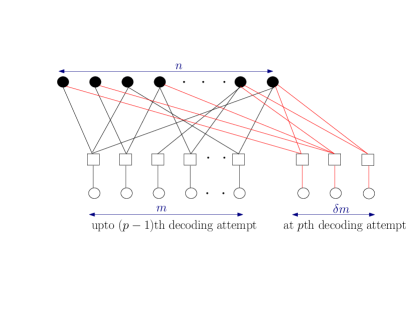
As stated earlier, a Raptor decoding process generally proceeds with several decoding attempts, where in each decoding attempt, Raptor decoding process runs a predetermined number of BP decoding iterations to obtain a message estimate. Specifically, the Raptor decoder begins the first decoding attempt after collecting $m_{f}$ number of received bits (i.e., the noise corrupted output bits). Then after the Raptor decoding process, it checks the errors in the recovered message using CRC bits embedded during LDPC encoding. If no error is found, i.e., the decoding attempt is successful, an acknowledgment is sent via a noiseless feedback channel and terminates the Raptor decoding process. If the first decoding attempt is not successful, Raptor decoder collects another $\delta m$ received bits and begins the second decoding attempt. This process is repeated until no error is found in the recovered message. In the Raptor decoding process, the size of the Tanner graph for a particular decoding attempt depends on the total number of output bits used in that decoding attempt. For example, at $p$th decoding attempt, the corresponding Tanner graph has $(n+m)$ variable nodes and $(n-k+m)$ check nodes, where $m=m_{f}+(p-1)\delta m$ (See Fig. 1(a)).

In this section, we consider two possible configurations for Raptor decoding process in the multi-edge framework: joint decoding scheme and tandem decoding scheme. Note that we use the message-reset decoding strategy throughout the paper unless otherwise stated.

III-A The joint decoding scheme based on the BP decoding and the MET-DE for Raptor codes

In joint decoding, LT and LDPC code components are decoded in parallel and provide extrinsic information to each other. One of the main advantages of representing Raptor codes in a multi-edge framework is that we can easily analyze joint decoding scheme based on the BP decoding using MET-DE.

In the BP decoding, there are three types of messages passing along the edges of the corresponding Tanner graph, namely channel message, variable-to-check message and check-to-variable message. The channel message is categorized as an intrinsic message, whereas the variable-to-check message and the check-to-variable message are categorized as extrinsic messages [21, pages 390-391]. Let $m_{\mathrm{v}\rightarrow\mathrm{c}}^{(\ell)}$ denote the variable-to-check message from variable node $\mathrm{v}$ to check node $\mathrm{c}$ at the $\ell{\text{th}}$ iteration of the BP decoding, $m_{\mathrm{c}\rightarrow\mathrm{v}}^{(\ell)}$ denote the check-to-variable message from check node $\mathrm{c}$ to variable node $\mathrm{v}$ at the $\ell{\text{th}}$ iteration of the BP decoding, and $m_{0}$ denote the channel message. For the $\ell{\text{th}}$ BP decoding iteration, $m_{\mathrm{v}\rightarrow\mathrm{c}}^{(\ell)}$ and $m_{\mathrm{c}\rightarrow\mathrm{v}}^{(\ell)}$ can be computed as follows:

$$m_{\mathrm{v}\rightarrow\mathrm{c}}^{(\ell)}=\begin{cases}m_{0}&\text{if~{}}\ell=1,\\ m_{0}+\sum_{\mathrm{c}^{\prime}\in C_{\mathrm{v}}\backslash\mathrm{c}}m_{\mathrm{c}^{\prime}\rightarrow\mathrm{v}}^{(\ell-1)}&\text{if~{}}\ell>1,\end{cases}$$ (12)

$$m_{\mathrm{c}\rightarrow\mathrm{v}}^{(\ell)} =2\tanh^{-1}\left(\prod_{\mathrm{v}^{\prime}\in V_{\mathrm{c}}\backslash\mathrm{v}}\tanh\left(\frac{m_{\mathrm{v}^{\prime}\rightarrow\mathrm{c}}^{(\ell)}}{2}\right)\right),$$ (13)

where $C_{\mathrm{v}}\backslash\mathrm{c}$ is the set of check nodes connected to variable node $\mathrm{v}$ excluding check node $\mathrm{c}$, and $V_{\mathrm{c}}\backslash\mathrm{v}$ is the set of variable nodes connected to check node $\mathrm{c}$ excluding variable node $\mathrm{v}$.

For the BP decoding on a BI-AWGN channel, intrinsic and extrinsic messages are described by PDFs for analysis using MET-DE. Let $f\big{(}{m_{\mathrm{v}\rightarrow\mathrm{c}}^{(\ell)}}\big{)}$ and $f\big{(}{m_{\mathrm{c}\rightarrow\mathrm{v}}^{(\ell)}}\big{)}$, respectively denote the PDF of the message from variable node $\mathrm{v}$ to check node $\mathrm{c}$ and, the PDF of the message from check node $\mathrm{c}$ to variable node $\mathrm{v}$, at the $\ell{\text{th}}$ BP decoding iteration. Let $f\big{(}m_{\mathrm{0}}\big{)}$ denote the PDF of the channel message. Then from (12) and (13), the updated message PDFs for variable nodes and check nodes at the $\ell$th BP decoding iteration can be computed as follows:

$$f\big{(}{m^{(\ell)}_{\mathrm{v}\rightarrow\mathrm{c}}}\big{)} =\begin{cases}f\big{(}m_{0}\big{)}&\text{if~{}}\ell=1,\\ f\big{(}m_{0}\big{)}\otimes\left[\stackrel{{\scriptstyle[}}{{\mathrm{}}}{c}^{\prime}\in C_{\mathrm{v}}\backslash\mathrm{c}]{}{\otimes}f\big{(}{m^{(\ell-1)}_{\mathrm{c}^{\prime}\rightarrow\mathrm{v}}}\big{)}\right]&\text{if~{}}\ell>1,\end{cases}$$ (14)

$$f\big{(}{m^{(\ell)}_{\mathrm{c}\rightarrow\mathrm{v}}}\big{)} =\stackrel{{\scriptstyle[}}{{\mathrm{}}}{v}^{\prime}\in V_{\mathrm{c}}\backslash\mathrm{v}]{}{\boxtimes}f\big{(}{m^{(\ell)}_{\mathrm{v}^{\prime}\rightarrow\mathrm{c}}}\big{)},$$ (15)

where $\otimes$ denotes the variable node convolution and $\boxtimes$ denotes the check node convolution. For more details we refer readers to Richardson and Urbanke [5, pages 390-391 and 459-478].

III-B Stability of Raptor codes with joint decoding using the multi-edge framework

The stability analysis using MET-DE examines the asymptotic behavior of the BP decoding when it is close to a successful decoding and gives a sufficient condition for the convergence of the bit error rate (BER) to zero as the BP decoding iteration, $\ell$, tends to infinity. Before analyzing the stability condition with the joint decoding scheme, we refer readers to Remark 1 and Lemma 1 given in Appendix A, upon which our analysis is based.

Now consider Raptor codes represented in a multi-edge framework. As shown in Fig. 1(b), the MET representation of a Raptor code has degree-one variable nodes. Therefore, messages on edge-types which are connected to degree-one variable nodes may not converge to zero BER even thought output BER converges to zero. Thus we need to consider the special case which is given in Remark 1. Recall that in the MET setting, a Raptor code is a serial concatenation of an LT code with an LDPC code. According to Remark 1, we can categorize edge-types in Fig. 1(b) as $E_{1}=\{\Pi_{1}\},~{}E_{2}=\{\Pi_{3}\}$ and $E_{1,2}=\{\Pi_{2}\}$ and define nodes connected to $\Pi_{1}$, i.e., the LDPC code component of the Raptor code, as the core LDPC graph for the stability analysis. The edge-perspective multinomial of the core LDPC graph with edges connected to $\Pi_{2}$ is given by

$$\lambda_{1}(x_{1},x_{2}) =\sum_{i\geq 2}\sum_{j\geq 1}\lambda_{[i~{}j]}~{}x_{1}^{i-1}~{}x_{2}^{j},$$ (16)

$$\rho_{1}(x_{1}) =\sum_{i\geq 0}\rho_{i}~{}x_{1}^{i-1},$$ (17)

where we assume that edges from $\Pi_{2}$, all carrying a fixed message PDF in check-to-variable direction. Since the stability analysis considers the termination of the BP decoding, i.e., $\ell\rightarrow\infty$, from Lemma 1, we can assume that edges from $\Pi_{2}$, all carry a message with the same distribution as the channel message in the check-to-variable direction. Then the stability condition for Raptor codes with joint decoding is given in Theorem 1.

Theorem 1 (Sufficient condition for the stability of Raptor codes decoded with joint decoding based on the BP decoding)

Consider a Raptor code decoded with a joint decoding based on the BP decoding using the multi-edge framework. On a BI-AWGN channel, the stability condition is given by

$$\sum_{j\geq 1}\lambda_{[2~{}j]}(x_{0})^{j}~{}\rho_{1}^{\prime}(1) <1,$$

where $\lambda_{[2~{}j]}$ gives the fraction of degree-two variable nodes in the LDPC code component and $x_{0}$ is the Bhattacharyya constant [5, pages 202] associated with the channel message with noise variance $\sigma^{2}$, and $\rho_{1}^{\prime}(1)=\frac{d\rho_{1}(x_{1})}{dx_{1}}\big{|}_{x_{1}=1}$.

Proof:

See Appendix B ∎

Note that Theorem 1 gives an upper bound on the fraction of degree-two variable nodes in the LDPC code component, which is similar to the stability condition of standard LDPC codes having multiple channel inputs.

III-C The tandem decoding scheme based on the BP decoding for Raptor codes using the multi-edge framework

Following the same procedure as for joint decoding, we can easily implement and analyze tandem decoding in the multi-edge framework using equations (12) to (15). The main difference between joint decoding and tandem decoding is that, in tandem decoding, LT and LDPC code components are decoded independently. That is at the first stage, we apply DE equations to the Tanner graph structure shown in Fig. 1(b) assuming that there are no messages coming from edge-type $\Pi_{1}$. Subsequently, once the predetermined criteria for the first stage is satisfied (such as the target minimum mean LLR ($\mu_{0}$) or the maximum number of BP decoding iterations for the LT code component), the decoded LLR of each input bit is computed as,

$$\mathcal{L}_{\mathrm{v}}=\sum_{\mathrm{c}\in C_{\mathrm{v}}}m_{\mathrm{c}\rightarrow\mathrm{v}}^{(\ell)},$$ (18)

where $\mathcal{L}_{\mathrm{v}}$ denotes the decoded LLR of input bit $\mathrm{v}$. At the second stage, we apply DE equations to the Tanner graph structure shown in Fig. 1(b) assuming that the check-to-variable messages coming from edge-type $\Pi_{2}$ are fixed and equal to the decoded LLRs.

III-D Stability of Raptor codes with tandem decoding using the multi-edge framework

In the stability analysis of tandem decoding, we generally examine the asymptotic behavior of the BP decoder at the beginning of the LT decoding process, assuming that the decoding of LDPC codes is successful. Thus the stability condition of Raptor codes with tandem decoding gives a condition to successfully start the BP decoding rather than the decoding convergence as in joint decoding. In this section, we validate the stability condition given in [12] for tandem decoding using the multi-edge framework.

The edge-perspective multinomial related to the LT code can be computed in the multi-edge framework as follows:

$$\lambda_{2}(x_{2}) =\frac{L_{x_{2}}(\boldsymbol{r},\boldsymbol{x})}{L_{x_{2}}(\boldsymbol{1},\boldsymbol{1})}=e^{\alpha(x_{2}-1)},$$ (19)

$$\rho_{2}(x_{2}) =\frac{R_{x_{2}}(\boldsymbol{x})}{R_{x_{2}}(\boldsymbol{1})}=\sum_{i}\left(\frac{i~{}\Omega_{i}}{\sum_{i}i~{}\Omega_{i}}\right)x_{2}^{i-1},$$ (20)

where $\Omega_{i}$ can be computed from (10). Etesami [12] showed that the input bit degree distribution is binomial and can be approximated by a Poisson distribution with parameter $\alpha$. Thus $\lambda_{2}(x_{2})$ is a Poisson distribution, where $\alpha$ is the average input bit degree. Then the stability condition for Raptor codes with tandem decoding is given in Theorem 2.

Theorem 2 (Stability of Raptor codes decoded with tandem decoding based on the BP decoding)

Consider a Raptor code decoded with tandem decoding based on the BP decoding using the multi-edge framework. Let $\Omega_{1}$ and $\Omega_{2}$, respectively denote the fractions of output bits with degree-one and degree-two, and $\alpha$ and $\beta$, respectively give the average degree of input bits and output bits. Then on a BI-AWGN channel, the BP decoding process can be started successfully, if $\Omega_{1}\geq 0$ and $\Omega_{2}\geq{\beta}/{2\alpha\tilde{x_{0}}}$, where $\tilde{x_{0}}$ is the D-mean [5, pages 201] associated with a channel message with noise variance $\sigma^{2}$. Moreover, for a capacity approaching code we have $\Omega_{2}\geq{C(\gamma)}/{2\tilde{x_{0}}}$, where $C(\gamma)$ is the capacity of the BI-AWGN channel with SNR, $\gamma$.

Proof:

See Appendix C ∎

To be more comprehensive, we also derive the stability condition for the LDPC code component of the Raptor code using MET-DE. In this case, we examine the asymptotic behavior of the BP decoding when it is close to a successful decoding, i.e., the BER of input bit nodes converge to zero. Recall that the edge-perspective degree distributions associated with the LDPC code is denoted by $\lambda(x)$ and $\rho(x)$. Under tandem decoding, LDPC code is decoded using decoded LLRs computed for each input bit node at the end of the LT decoding process. In the stability analysis we consider these decoded LLRs as channel inputs to each input bit node. Then the stability condition for LDPC code component of the Raptor code with tandem decoding is given in Theorem 3.

Theorem 3 (Sufficient condition for the stability of the LDPC code component of the Raptor code decoded with tandem decoding based on the BP decoding )

Consider a Raptor code decoded with tandem decoding based on the BP decoding using the multi-edge framework. On a BI-AWGN channel, the decoding of the LDPC code component of the Raptor code is successful if $\lambda_{2}~{}\rho^{\prime}(1)\leq 1/\mathcal{B}(\mathcal{L}_{2})$, where $\lambda_{2}$ gives the fraction of degree-two variable nodes (i.e., degree-two input bit nodes) in the LDPC code component and $\mathcal{B}(\mathcal{L}_{2})$ is the Bhattacharyya constant [5, pages 202] associated with the decoded LLR of input bit nodes with degree-two.

Proof:

We can proceed the same way as with Theorem 1 to complete the proof. ∎

III-E Tandem decoding scheme based on the incremental decoding strategy

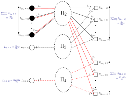
In this section, we implement the incremental decoding strategy for tandem decoding using the multi-edge framework. The difference between the message-reset decoding strategy and the incremental decoding strategy is the way that they initialize the BP decoding algorithm for the LT decoding process. That is, with the incremental decoding strategy, the initial variable-to-check messages (i.e., when $\ell=1$) passed in the LT decoding process at the $p$th decoding attempt is set to the corresponding messages computed at the end of the $(p-1)$th decoding attempt [11], whereas with the message-reset decoding strategy these initial variable-to-check messages are initialized to zero at every decoding attempt. Under the incremental decoding strategy, the initial variable-to-check messages passed in the LT decoding process at the $p$th decoding attempt ($m_{\mathrm{v}\rightarrow\mathrm{c}}^{(\ell=1)}$) can be computed as follows:

$$m_{\mathrm{v}\rightarrow\mathrm{c}}^{(\ell=1)}=\begin{cases}m_{0}&\text{\small for a new variable node},\\ m_{0}+\sum_{\mathrm{c}^{\prime}\in C_{\mathrm{v}}\backslash\mathrm{c}}m_{\mathrm{c}^{\prime}\rightarrow\mathrm{v}}^{(T)}&\text{\small for a variable node used in previous decoding attempt},\end{cases}$$ (21)

where $m_{\mathrm{c}^{\prime}\rightarrow\mathrm{v}}^{(T)}$ denotes the check-to-variable message computed at the end of the $(p-1)$th decoding attempt. Moreover in our implementation, we propose a modification to incremental decoding strategy, where we only use a fraction of output bits received during the previous decoding attempts in order to further minimize the decoding complexity of the incremental decoding strategy. As shown in Fig. 2, we implement the incremental decoding strategy using three edge-types (for the LT code component), where the $m$ output bits received during previous decoding attempts are connected to edge-type $\Pi_{3}$, and the $\delta m$ new output bits received at the current decoding attempt are connected to edge-type $\Pi_{4}$. We use $x$ to denote the fraction of output bits used from the previous decoding attempts. The parameter $x$ can be used as a controlling parameter to trade–off between performance and decoding complexity and $x$ can take values from 0 to 1, where $x=1$ corresponds to traditional incremental decoding.

(a) An example Tanner graph of the LT code component of a Raptor code truncated at code length $m+\delta m$.

(b) The Tanner graph of the LT code component of the Raptor code ensemble as a MET-LDPC code ensemble for incremental decoding strategy.

Figure 2: Graphical representation of the LT code component of the Raptor code ensemble at $p$th decoding attempt with incremental decoding strategy using the multi-edge framework. $x$ denotes the fraction of output bits used from previous decoding attempts. $\mathcal{R}_{1}$ and $\mathcal{R}_{2}$ respectively denote realized rates at the $(p-1)$th decoding attempt and the $p$th decoding attempt. Not shown are the ($1-x$) fraction of output bit nodes not used in this decoding round.

IV Design of Raptor codes in the MET framework

IV-A Problem statement for Raptor code optimization in the multi-edge framework

For the Raptor code optimization, we consider a Raptor code as a MET-LDPC code, and formulate the optimization problem to maximize the design rate, $\mathcal{R}(\gamma)$, for a given channel SNR, $\gamma$, and maximum check node degrees, $i_{c_{\max}}$ and $j_{c_{\max}}$, such that the BER of variable nodes decreases through BP decoding iterations. One of the main features of the proposed optimization method is that we jointly optimize the LT and the LDPC code components. We can formulate the optimization problem for the Raptor code in the multi-edge framework using joint decoding scheme as follows:

For a given SNR, $\gamma$, and maximum check node degrees, $i_{c_{\max}}$ and $j_{c_{\max}}$,

$$\begin{aligned} &{\mathrm{Maximize}}&&\mathcal{R}(\gamma)\\ &\mathrm{Subject~{}to}&&(i)~{}L_{[0~{}0~{}1]}=1,\\ &&&(ii)~{}\sum_{j_{c}=1}^{j_{c_{\max}}}R_{[0~{}j_{c}~{}1]}=1,\\ &&&(iii)~{}L(\boldsymbol{1},\boldsymbol{1})-R(\boldsymbol{1})=\mathcal{R}(\gamma),\\ &&&(iv)~{}L_{x_{i}}(\boldsymbol{1},\boldsymbol{1})=R_{x_{i}}(\boldsymbol{1}),\\ &&&(v)~{}\max_{j}\{P_{j}\}<P^{*},\end{aligned}$$ (22)

where $P_{j}$ and $P^{*}$ respectively denote the BER on the $j$th variable node and target maximum BER. Here $\mathcal{R}(\gamma)$ can be determined using MET-DE. Note that constraints $(i)$ and $(ii)$ were described in (3) and (4), constraint $(iii)$ imposes the code rate, constraint $(iv)$ is to satisfy the total number of edges of each edge-type in variable node side and check node side. This is known as the socket count equality constraint, where

$$L_{x_{i}}(\boldsymbol{1},\boldsymbol{1})=\frac{dL(\boldsymbol{r},\boldsymbol{x})}{d{x_{i}}}\biggr{|}_{\boldsymbol{r}=\boldsymbol{1},\boldsymbol{x}=\boldsymbol{1}}\hskip 28.45274pt\text{and}\hskip 28.45274ptR_{x_{i}}(\boldsymbol{1})=\frac{dR(\boldsymbol{x})}{d{x_{i}}}\biggr{|}_{\boldsymbol{x}=\boldsymbol{1}}.$$

Finally, constraint $(v)$ is to make sure that the MET-DE returns a smaller BER than the predefined BER value.

IV-B Problem statement for Raptor code optimization for fixed precode settings

In the majority of literature concerning Raptor code design, the precode is fixed in advance (usually a high-rate regular or irregular LDPC code) and only the LT code is optimized for a given precode setting, using linear programming based on approximate DE algorithms. Therefore, for a fair comparison with the existing results in literature, we reformulate the optimization problem given in (22), where we optimize the Raptor code using the multi-edge framework and the MET-DE to maximize the design rate of the LT code, $\mathcal{R}_{\mathrm{LT}}$ (i.e., only $L_{x_{2}}$ and $R_{x_{2}}$ are optimized). This is equivalent to maximizing the design rate of Raptor code $\mathcal{R}(\gamma)$ for a given LDPC code rate, $\mathcal{R}_{\mathrm{LDPC}}$.

The reformulated optimization problem for the Raptor code with fixed precode settings in the multi-edge framework using joint decoding scheme is as follows:

For a given SNR, $\gamma$, maximum check node degree, $j_{c_{\max}}$, and LDPC code rate, $\mathcal{R}_{\mathrm{LDPC}}$,

$$\begin{aligned} &{\mathrm{Maximize}}&&\mathcal{R}_{\mathrm{LT}}\\ &\mathrm{Subject~{}to}&&(i)~{}L_{[0~{}0~{}1]}=1,\\ &&&(ii)~{}\sum_{j_{c}=1}^{j_{c_{\max}}}R_{[0~{}j_{c}~{}1]}=1,\\ &&&(iii)~{}\sum_{i_{v}=1}^{i_{v_{\max}}}~{}\sum_{j_{v}=1}^{j_{v_{\max}}}L_{[i_{v}~{}j_{v}~{}0]}=\mathcal{R}_{\mathrm{LT}},\\ &&&(iv)~{}\sum_{i_{c}=1}^{{i_{c_{\max}}}}R_{[i_{c}~{}0~{}0]}=\mathcal{R}_{\mathrm{LT}}(1-\mathcal{R}_{\mathrm{LDPC}}),\\ &&&(v)~{}L_{x_{2}}(\boldsymbol{1},\boldsymbol{1})=R_{x_{2}}(\boldsymbol{1}),\\ &&&(vi)~{}\max_{j}\{P_{j}\}<P^{*}.\end{aligned}$$ (23)

Here $\mathcal{R}_{\mathrm{LT}}$ can be determined using MET-DE and constraints $(iii)$ and $(iv)$ described in (5) and (6), which are used to impose the rates of LT and LDPC codes into the multi-edge framework. Note that if we use the tandem decoding scheme, we need an additional constraint on the $\mu_{0}$ (or maximum number of BP decoding iterations in the LT decoder) to determine when the BP decoding process will be switched from LT decoder to LDPC decoder.

IV-C Optimization of the degree distribution in the multi-edge framework

Recall that the degree distributions of the Raptor code ensemble in the multi-edge framework are denoted by $L(\boldsymbol{r},\boldsymbol{x})$ and $R(\boldsymbol{x})$. As stated in Sections IV-A and IV-B, our goal in the Raptor code optimization is to optimally choose the elements in $L(\boldsymbol{r},\boldsymbol{x})$ and $R(\boldsymbol{x})$ so that the corresponding code ensemble yields the largest possible realized rate, which can be determined via MET-DE. We employ a combined optimization method proposed in [22] to optimize MET-LDPC code ensembles to that Raptor code ensembles which are represented in the multi-edge framework. The combined optimization method optimizes the node fractions (denoted by $L_{[i_{v}~{}j_{v}~{}k_{v}]}$ and $R_{[i_{c}~{}j_{c}~{}k_{c}]}$ in (1) and (2) ) and the node degrees (denoted by $[i_{v}~{}j_{v}~{}k_{v}]$ and $[i_{c}~{}j_{c}~{}k_{c}]$ in (1) and (2)) in parallel using two different optimization techniques. In this work, we use adaptive range method [22] to optimize the node fractions and differential evolution [23] to optimize the node degrees.

IV-C1 Input bit node degree distribution

The aim of the Raptor code optimization in multi-edge framework is to optimally choose $L(\boldsymbol{r},\boldsymbol{x})$ and $R(\boldsymbol{x})$ so that the corresponding code ensemble yields the largest possible realized rate. Under multi-edge framework, there are two essential constraints that needs to be satisfied in order to have a valid Raptor code degree distribution, namely the code rate constraint and the socket count equality constraint. These two constraints allow us to include $L(\boldsymbol{r},\boldsymbol{x})$ (i.e., $L_{[i_{v}~{}j_{v}~{}k_{v}]}$ and $[i_{v}~{}j_{v}~{}k_{v}]$) as dependent variables in the code optimization. In our design method, we choose two or three non-zero variable node degrees (which may be chosen consecutively) for the $L(\boldsymbol{r},\boldsymbol{x})$, based on $R(\boldsymbol{x})$ in order to achieve the desired code rate. Because, as shown by Hussain et al. [24], we have also observed that there is a little difference in performance whether $L(\boldsymbol{r},\boldsymbol{x})$ is almost-regular or Poisson. At the same time, selecting an almost regular input bit degree distribution significantly helps to minimize the computational complexity of MET-DE, which in turn helps for an efficient code optimization.

IV-D A remark on Raptor code design

IV-D1 Selecting $\mu_{0}$ for tandem decoding

In the majority of literature concerning Raptor code design, which use tandem decoding to formulate the optimization problem, $\mu_{0}$ plays an important role. However no serious effort has been taken for deriving the optimal choice of $\mu_{0}$ and it remains mostly heuristic. We have investigated the optimal choice of $\mu_{0}$ using the multi-edge framework and observed that the choice of $\mu_{0}$ depends on the rate and the structure of the LDPC code selected for the precode and the channel SNR. Here we explain the reasons behind this.

There are two important requirements that needs to be satisfied when we are selecting a value for $\mu_{0}$. The first requirement is that the value of $\mu_{0}$ needs to be selected based on the target residual error which is expected to be corrected by the LDPC decoder. The second requirement is that $\mu_{0}\leq\min(\mathcal{L}_{\mathrm{v}})$ in order to ensure a successful decoding at the LDPC decoder. The first requirement concludes that the choice of $\mu_{0}$ depends on the rate and structure of the LDPC code as the error correcting performance of a code is approximately determined by these two parameters.

We then use Lemma 1 in Appendix A to explain the second requirement. As shown in Fig. 1(b), the LT code component in MET setting has a set of degree-one variable nodes. Therefore according to Lemma 1, after a sufficient number of BP decoding iterations at the LT decoder, the check-to-variable message from an output check node, $m_{\mathrm{c}\rightarrow\mathrm{v}}^{(\ell)}$, is converging to the same distribution as the channel message received at the output bit nodes, $m_{0}$. Thus, the decoded LLR of input bit node $\mathrm{v}$ given in (18) can be rewritten as $\mathcal{L}_{\mathrm{v}}=\sum_{\mathrm{c}\in C_{\mathrm{v}}}m_{0}$. Moreover, condition $\min(\mathcal{L}_{\mathrm{v}})\geq\mu_{0}$ must hold to ensure a successful decoding at the LDPC decoder. This alternatively shows that the value of $\mu_{0}$ depends on the distribution of the channel message received at the output bit nodes, which is a symmetric Gaussian distribution with mean, $2\gamma$, and variance, $4\gamma$, where $\gamma$ is the channel SNR.

IV-D2 Selection of the LDPC code rate

Previous work concerning Raptor code design appears to have overlooked the choice of LDPC code rate and have selected an arbitrary LDPC code rate as long as the rate loss is not significant. Mostly Raptor code designers have selected higher rates for the LDPC code such as 0.98 or 0.95 due to very small rate loss. Cheng et al. [13] showed that a Raptor code with a rate-0.7 LDPC code perform poorly compared to a Raptor code with a rate-0.95 LDPC code, particularly at high SNRs. This mainly due to the severe rate loss in the low-rate precoding. Generally, at a higher SNR, an LDPC code only performs error detection rather than error correction. Thus the use of low-rate precoding at high SNRs will result in severe rate loss. In contrast, at a lower SNR, a low-rate LDPC code can perform both error detection and error correction, thus can help to increase the realized rate of the LT code component. However, in general the rate gain obtain from low rate precoding is insignificant compared to the rate loss in the entire Raptor code due to low rate precoding. Thus Raptor code designers always encourage to use high-rate LDPC code for precoding.

V Results and Discussion

V-A Performance comparison of Raptor codes designed using the multi-edge framework and tandem decoding with existing Raptor code results

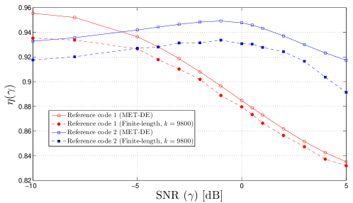
In this section, we compare the performance of Raptor codes designed with the optimization method given in Section IV-B using the multi-edge framework, with the existing Raptor codes in literature. For a fair comparison, we set same precode settings as the reference codes and use tandem decoding scheme as the decoding scheme in the code optimization. We consider two reference codes from literature, where reference code 1 [10] was designed with precode rate of 0.98 for very low SNRs and reference code 2 [12] was designed with precode rate of 0.98 at SNR 0.5 dB. We use (4, 200)-regular LDPC code as the precode and set maximum number of BP decoding iterations to 1000. We use the maximum average message mean, $\mu_{0}$, as the switching criterion from LT code component to LDPC code component with tandem decoding and set the value of $\mu_{0}$ to 40 for optimized code 1 and 30 for optimized code 2. In MET-DE we set the number of sample points in the quantization to 3000 and the quantization interval to 0.01.

In order to verify the correctness of MET-DE for Raptor code analysis, we first compare the rate efficiency results computed with MET-DE and finite-length simulations for the existing Raptor codes in literature in Fig. 3. It is clear from Fig. 3 that the rate efficiency results computed with MET-DE closely follow the finite-length simulations at all SNRs. We then compare the rate efficiency result of the Raptor codes designed in the multi-edge framework using tandem decoding, with the existing Raptor codes in literature in Table I. It is clear from Table I that optimized Raptor codes using the multi-edge framework give higher rate efficiencies than reference codes. Moreover, optimized codes have smaller maximum output check node degree compared to reference codes. The advantage of having lower degrees in a code ensemble is that it helps to reduce the decoding complexity.

TABLE I: Comparison of optimized Raptor code degree distributions with existing Raptor code degree distributions

Design	Raptor code	Degree distribution	Avg. output	$\eta(\gamma_{d})$
SNR ($\gamma_{d}$)			node degree ($\beta$)	(MET-DE)
-10 dB	Reference code 1	$\Omega(x)=0.0174\,x+0.3488\,x^{2}+0.2309\,x^{3}+0.0695\,x^{4}+0.0873\,x^{5}$	14.01	0.9556
	[10, Table II]	$+0.0002\,x^{6}+0.0805\,x^{7}+0.0004\,x^{8}+0.0191\,x^{11}+0.0518\,x^{12}$
		$+0.0123\,x^{23}+0.031\,x^{24}+0.022\,x^{59}+0.002\,x^{60}+0.02683\,x^{300}$
	Optimized code 1	$\Omega(x)=0.0261\,x+0.3526\,x^{2}+0.3195\,x^{3}+0.0946\,x^{5}+0.0076\,x^{6}$	6.68	0.9606
$+0.1508\,x^{12}+0.0055\,x^{16}+0.002\,x^{19}+0.008\,x^{23}+0.0091\,x^{61}$
	$+0.023\,x^{63}+0.00123\,x^{290}$
0.5 dB	Reference code 2	$\Omega(x)=0.0006\,x+0.492\,{x}^{2}+0.0339\,{x}^{3}+0.2403\,{x}^{4}+0.006\,{x}^{5}$	11.16	0.9458
	[12, Page 2044]	$+0.095\,{x}^{8}+0.049\,{x}^{14}+0.018\,{x}^{30}+0.0356\,{x}^{33}+0.0296\,{x}^{200}$
	Optimized code 2	$\Omega(x)=0.0082\,x+0.5019\,x^{2}+0.043\,x^{3}+0.2365\,x^{4}+0.0067\,x^{5}$	11.47	0.9524
		$+0.0911\,x^{8}+0.0398\,x^{14}+0.0108\,x^{30}+0.0273\,x^{33}+0.0347\,x^{197}$

Figure 3: Rate efficiency results computed using MET-DE and finite-length simulations for the existing Raptor codes in literature with fixed LDPC code rate of 0.98, evaluated at different SNRs.

V-B Tandem decoding vs. joint decoding

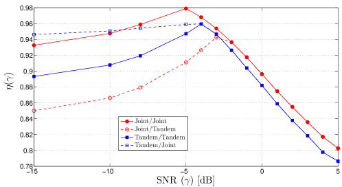
In this section, we consider the design of Raptor codes for a given precode rate using tandem and joint decoding schemes. We formulate the optimization problem as per Section IV-B and set the precode to a (3,60)-regular LDPC code of rate 0.95, and maximum check node degree, $j_{c_{\max}}$, to 50. In Fig. 4 we show the rate efficiency results of the Raptor code degree distributions designed using joint and tandem decoding schemes for different SNRs. Note that each point in the figure corresponds to a code designed specifically for that SNR. It can be observed that Raptor codes designed using joint decoding always outperform Raptor codes designed using tandem decoding in terms of rate efficiency. However, as the designed SNR increases, the rate efficiency gap between Raptor codes designed with joint decoding and tandem decoding is reduced. Furthermore with joint decoding, the BP decoding algorithm converges to a zero BER faster than with tandem decoding, which improves the rate efficiency. Additional advantages of joint decoding is that we no longer need to consider the switching point between LT code component to LDPC code component, and we can use the LDPC code parity-check to halt decoding early once a valid codeword is found.

Figure 4: Rate efficiency results computed using MET-DE for the Raptor codes designed using the multi-edge framework, evaluated at the designed SNR.

In Table II we compare the rate efficiency results computed using MET-DE for the optimized Raptor codes shown in Fig. 4 with fixed LDPC code rate of 0.95, designed/evaluated using joint decoding and tandem decoding at the designed SNR. It is clear from Table II that Raptor codes designed and/or evaluated using joint decoding always show the best rate efficiency performance. Moreover in Fig. 5, we evaluate the rate efficiency performance of optimized degree distributions designed at -5 dB (which are shown in Fig. 4 with fixed LDPC code rate of 0.95) for SNRs above and below the designed SNR using tandem decoding and joint decoding. It can be observed from Fig. 5 that Raptor codes evaluated using joint decoding always show the best rate efficiency performance regardless of whether the code was optimized with joint or tandem decoding. This seems to be significant when the evaluated SNR is below the designed SNR. The reason is that the use of the information generated from both LT and LDPC code components in parallel helps to minimize the residual error; thus improving the rate efficiency performance.

TABLE II: Rate efficiency results computed using MET-DE for the optimized Raptor codes shown in Fig. 4 with fixed LDPC code rate of 0.95, designed/evaluated using joint decoding and tandem decoding at the designed SNR.

Designed	$\eta(\gamma_{d})$ (MET-DE)
SNR ($\gamma_{d}$)	Joint/Joint	Joint/Tandem	Tandem/Tandem	Tandem/Joint
-10 dB	0.9864	0.9053	0.9529	0.9571
-5 dB	0.9783	0.9112	0.9472	0.9590
0 dB	0.9773	0.9173	0.9455	0.9633
5 dB	0.9609	0.9159	0.9413	0.9541
10 dB	0.9530	0.9174	0.9380	0.9472

Figure 5: Rate efficiency results computed using MET-DE for the Raptor codes designed at -5dB with fixed LDPC code rate of 0.95, designed/evaluated using joint decoding and tandem decoding.

V-C The Raptor codes design as MET-LDPC codes using joint decoding

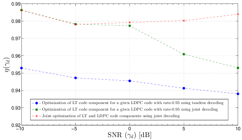
In this section, we consider the design of Raptor codes as MET-LDPC codes, where we do not fix the rate and the structure of the precode in advance. We formulate the optimization problem as per Section IV-A. The main advantage of this method is that, it allows us to select the most suitable precode setting depending on the design SNR.

The degree distributions of Raptor codes designed with the multi-edge framework using joint decoding scheme for different SNRs are given in Table III. We present the degree distributions using MET notations as we design them as MET-LDPC codes. One can easily compute the relevant $\Omega(x)$ and the degree distributions of LDPC code using (10) and (11). In Fig. 4 we show the rate efficiency results for the optimized Raptor codes given in Table III to compare the rate efficiency results obtained with fixed precode setting. It is clear from results shown in this section that the Raptor codes designed using the multi-edge framework achieve realized rates close to the channel capacity for any channel SNR (Indeed codes can be designed at any SNR regardless of whether joint or tandem decoding is considered). Therefore, the proposed method using the multi-edge framework succeeds to overcome the problem in existing linear programming based on mean-LLR-EXIT chart method [12, 13], where it is only capable of giving the capacity achieving codes between two SNR bounds $\text{SNR}^{*}_{\text{low}}$ and $\text{SNR}^{*}_{\text{high}}$ given in [13].

TABLE III: Optimized degree distributions of Raptor codes as MET-LDPC codes for different designed SNRs using joint decoding

Designed	Raptor code as a MET-LDPC code	$\mathcal{R}_{\text{LDPC}}$	$\eta(\gamma_{d})$
SNR ($\gamma_{d}$)			(MET-DE)
-10 dB	$L(\boldsymbol{r},\boldsymbol{x})=0.0445\,{x_{1}}^{3}\,{x_{2}}^{61}+0.0268\,{x_{1}}^{3}\,{x_{2}}^{62}+x_{3}$	0.9500	0.9862
	$R(\boldsymbol{x})=0.0036\,{x_{1}}^{60}+0.0117\,x_{2}\,x_{3}+0.3616\,{x_{2}}^{2}\,x_{3}+0.3005\,{x_{2}}^{3}\,x_{3}+0.0958\,{x_{2}}^{4}\,x_{3}$
$+0.0952\,{x_{2}}^{7}\,x_{3}+0.0344\,{x_{2}}^{9}\,x_{3}+0.046\,{x_{2}}^{12}\,x_{3}+0.0389\,{x_{2}}^{12}\,x_{3}+0.0149\,{x_{2}}^{21}\,x_{3}$
$+0.001\,{x_{2}}^{50}\,x_{3}$
-5 dB	$L(\boldsymbol{r},\boldsymbol{x})=0.054\,{x_{1}}^{3}\,{x_{2}}^{19}+0.1506\,{x_{1}}^{3}\,{x_{2}}^{20}+x_{3}$	0.9450	0.9781
	$R(\boldsymbol{x})=0.006139\,{x_{1}}^{55}+0.0051\,{x_{1}}^{54}+0.0436\,x_{2}\,x_{3}+0.3796\,{x_{2}}^{3}\,x_{3}+0.2738\,{x_{2}}^{2}\,x_{3}$
$+0.0048\,{x_{2}}^{4}\,x_{3}+0.0386\,{x_{2}}^{2}\,x_{3}+0.022\,{x_{2}}^{3}\,x_{3}+0.1211\,{x_{2}}^{10}\,x_{3}+0.1057\,{x_{2}}^{6}\,x_{3}$
$+0.0104\,{x_{2}}^{27}\,x_{3}+0.0004\,{x_{2}}^{50}\,x_{3}$
0 dB	$L(\boldsymbol{r},\boldsymbol{x})=0.0047\,{x_{1}}^{3}\,{x_{2}}^{6}+0.4904\,{x_{1}}^{3}\,{x_{2}}^{7}+x_{3}$	0.9610	0.97923
	$R(\boldsymbol{x})=0.0178\,{x_{1}}^{77}+0.0014\,{x_{1}}^{76}+0.0318\,x_{2}\,x_{3}+0.3955\,{x_{2}}^{2}\,x_{3}+0.2926\,{x_{2}}^{3}\,x_{3}$
$+0.0738\,{x_{2}}^{3}\,x_{3}+0.0711\,{x_{2}}^{3}\,x_{3}+0.0575\,{x_{2}}^{9}\,x_{3}+0.0528\,{x_{2}}^{9}\,x_{3}+0.0236\,{x_{2}}^{12}\,x_{3}$
$+0.0006\,{x_{2}}^{25}\,x_{3}+0.0007\,{x_{2}}^{50}\,x_{3}$
5 dB	$L(\boldsymbol{r},\boldsymbol{x})=0.1122\,{x_{1}}^{2}\,{x_{2}}^{3}+0.1295\,{x_{1}}^{3}\,{x_{2}}^{3}+0.6092\,{x_{1}}^{3}\,{x_{2}}^{4}+x_{3}$	0.9898	0.9802
	$R(\boldsymbol{x})=0.0014\,{x_{1}}^{297}+0.0016\,{x_{1}}^{297}+0.0025\,{x_{1}}^{300}+0.0026\,{x_{1}}^{299}+0.0005\,{x_{1}}^{44}$
$+0.0915\,x_{2}\,x_{3}+0.3848\,{x_{2}}^{2}\,x_{3}+0.4328\,{x_{2}}^{3}\,x_{3}+0.026\,{x_{2}}^{4}\,x_{3}+0.0109\,{x_{2}}^{7}\,x_{3}$
$+0.0258\,{x_{2}}^{10}\,x_{3}+0.0282\,{x_{2}}^{20}\,x_{3}$
10 dB	$L(\boldsymbol{r},\boldsymbol{x})=0.3301\,x_{1}\,{x_{2}}^{2}+0.297\,x_{1}\,{x_{2}}^{3}+0.3604\,{x_{1}}^{2}\,{x_{2}}^{3}+x_{3}$	0.9932	0.9840
	$R(\boldsymbol{x})=0.0024\,{x_{1}}^{242}+0.0021\,{x_{1}}^{80}+0.0015\,{x_{1}}^{300}+0.0001\,{x_{1}}^{232}+0.0006\,{x_{1}}^{210}$
$+~{}0.0543\,x_{2}\,x_{3}+0.6645\,{x_{2}}^{2}\,x_{3}+0.1362\,{x_{2}}^{3}\,x_{3}+0.0943\,{x_{2}}^{4}\,x_{3}+0.0367\,{x_{2}}^{5}\,x_{3}$
$+0.014\,{x_{2}}^{20}\,x_{3}$

V-D Incremental decoding strategy for Raptor codes designed using tandem decoding scheme

This section considers the incremental decoding strategy for Raptor codes. For simplicity, we assume that all decoding attempts are uniformly spaced, i,e., the number of extra output bits ($\delta m$) received at each decoding attempt is the same. This is true for both message-reset decoding and incremental decoding. We also assume that the LT decoding process will perform a predetermined number of BP decoding iterations ($T$). The decoding complexity of the message-reset decoding and incremental decoding is given in Table IV. This gives the number of floating point operations per decoding attempt, which is also the number of convolutions involved in the MET-DE. It is clear from Table IV that the incremental decoding strategy has a lower decoding complexity compared to the message-reset decoding, because the Tanner graph corresponding to incremental decoding has a smaller number of edges compared to the one with message-reset decoding. Note that if we set $x$ to one, then the decoding complexity of the check node side is the same for both incremental decoding and message-reset decoding.

TABLE IV: Floating point operations per decoding attempt for the LT code component of the Raptor code

Decoding strategy	Variable nodes	Check nodes
Message-reset decoding	$(ni_{v}+m+\delta m)T$	$(mj_{c}+\delta md_{c})T$
Incremental decoding	$(n\bar{i}_{v}+xm+\delta m)T$	$(xm\bar{j}_{c}+\delta m\bar{d}_{c})T$

• $i_{v}$, $j_{c}$ and $d_{c}$ respectively denote the average degree of input bit nodes, average degree of output check nodes received during previous decoding attempts and the average degree of output check nodes received at the current decoding attempt for message-reset decoding.

• $\bar{i}_{v}$, $\bar{j}_{c}$ and $\bar{d}_{c}$ respectively denote the average degree of input bit nodes, average degree of the fraction of output check nodes selected from previous decoding attempts and the average degree of output check nodes received at the current decoding attempt for incremental decoding. Note that $i_{v}>\bar{i}_{v}$ and $j_{c}>\bar{j}_{c}$ for $x<1$.

Figure 6: Rate efficiency performance of the Raptor code designed at 0 dB with tandem decoding scheme for fixed precode settings in Section V-B, evaluated with incremental decoding strategy.

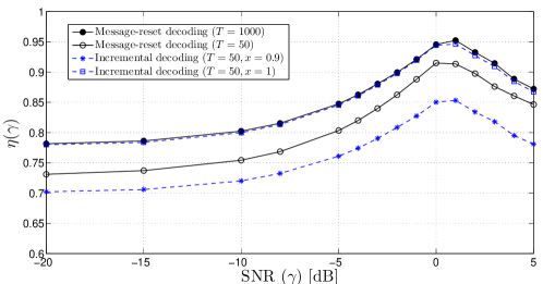
We then evaluate the performance of these two decoding strategies using the rate efficiency results. We consider the Raptor code designed at 0 dB with tandem decoding scheme for fixed precode settings in Section V-B, which has LT degree distribution of

$$\Omega(x)=0.0135x+0.4920x^{2}+0.2836x^{3}+0.0538x^{5}+0.0499x^{8}+0.0779x^{9}+\\ 0.0287x^{19}+0.0006x^{50}$$ (24)

In Fig. 6 we show the rate efficiency results for (24) decoded with the incremental decoding strategy. For a fair comparison, we also show the rate efficiency results for (24) decoded with message-reset decoding using the same number of BP decoding iterations ($T$). It is clear from Fig. 6 that incremental decoding ($T=50$ and $x=1$) outperforms message-reset decoding ($T=50$) with the same decoding complexity. Moreover, we can obtain rate efficiency results close to the optimal result (i.e., message-reset decoding with $T=1000$, where we have chosen $T=1000$ as increasing $T$ beyond 1000 does not noticeably improve $\eta(\gamma)$) by having incremental decoding of $T=50,x=1$, which offers a significant reduction of the decoding complexity. This is mainly due to the fact that recalculation of the same information is avoided with the incremental decoding. Therefore, we can suggest that incremental decoding closely approximate the optimal decoding strategy for the Raptor code design, where accurate and efficient rate calculation is particularly valuable.

VI Conclusion

In this paper, we proposed a new representation of Raptor codes as a multi-edge type low-density parity-check (MET-LDPC) code. This MET representation enable us to perform a comprehensive analysis of asymptotic performance of the Raptor code using MET density evolution (MET-DE). The advantage of using MET-DE over conventional Gaussian approximation-based approaches, such as mean-LLR-EXIT chart, is that MET-DE does not incorporate any Gaussian approximation, thus enables to find the optimal Raptor code for given channel condition. In addition, unlike finite-length analysis MET-DE gives the average performance of Raptor code ensemble. We considered two decoding schemes based on the belief propagation decoding, namely tandem decoding and joint decoding in the multi-edge framework, and analyzed the stability conditions using MET-DE. We then formulated the optimization problem to design Raptor codes using the multi-edge framework. Finally, we considered performance–complexity trade–offs of Raptor codes using the multi-edge framework. The density evolution analysis showed that Raptor codes designed with joint decoding always outperform the ones designed with tandem decoding. In several examples, we demonstrated that Raptor codes designed using the multi-edge framework outperform previously reported Raptor codes.

Appendix A

Lemma 1 (Degree-one variable nodes [4])

Any check node that receives information from a degree-one variable node outputs a check-to-variable message with the distribution $\Delta$ in all the edges except the edge which connects to the degree-one variable node if that check node receives messages from its connected variable nodes with a distribution of infinitely large mean. The distribution $\Delta$ is converging to the same distribution as the channel message received to its connected degree-one variable node as the number of BP decoding iterations goes to infinity.

Proof:

Consider a set of independent random variables $x_{1}\dots x_{n}$, and let $\mathcal{L}(x_{i})$ denote the corresponding LLR value of random variable $x_{i}$. Then the modulo-2-sum of LLRs of $x_{1}\dots x_{n}$ is $\mathcal{L}(x_{1})\oplus\mathcal{L}(x_{2})\oplus\dots\oplus\mathcal{L}(x_{n})=\mathcal{L}(x_{1}\oplus x_{2}\oplus\dots\oplus x_{n})$ and $\mathcal{L}(x_{1}\oplus x_{2}\oplus\dots\oplus x_{n})\stackrel{{\scriptstyle p}}{{\rightarrow}}\mathcal{L}(x_{1})$ as $\min_{2\leq i\leq n}\mathbb{E}[\mathcal{L}(x_{i})]\rightarrow\infty$. ∎

Remark 1 (Stability of MET-LDPC codes with degree-one variable nodes [5, pages 396-397])

Consider a MET-LDPC code having no degree-one variable nodes together with its serial concatenation with LDGM code. We refer the sub-Tanner graph having no degree-one variable nodes as the Core LDPC graph. Let $E_{1}$ denote the set of edge-types in the core LDPC graph, $E_{2}$ denote the set of edge-types attached exclusively to degree-one variable nodes and $E_{1,2}$ denote the set of edge-types which connect variable nodes in the core LDPC graph to the check nodes associated to the LDGM code. Then if the perfectly decodable fixed point of the core LDPC graph is stable with the PDFs carried on edge-type $E_{1,2}$ in check-to-variable direction, then the fixed point associated to the full graph is stable.

Appendix B Proof of Theorem 1

Let $a_{i}^{(\ell)}$ and $b_{i}^{(\ell)}$ respectively denote the PDFs of variable-to-check message and check-to-variable message along $\Pi_{i}$ at the $\ell$th BP decoding iteration. Let $x_{i}^{(\ell)}$ and $y_{i}^{(\ell)}$ respectively denote the Bhattacharyya constants [5, pages 202] associated with $a_{i}^{(\ell)}$ and $b_{i}^{(\ell)}$. Note that $\Pi_{1}$ represents the core LDPC graph. Using equations (14) and (15) we can write DE equations related to variable nodes and check nodes of the core LDPC graph as follows:

$$a_{1}^{(\ell+1)} =\sum_{i\geq 2}\sum_{j\geq 1}\lambda_{[i~{}j]}\left[b_{1}^{(\ell)}\right]^{\otimes(i-1)}\otimes\left[b_{2}^{(\ell)}\right]^{\otimes(j)}=\lambda_{1}(b_{1}^{(\ell)},b_{2}^{(\ell)}),$$ (25)

$$b_{1}^{(\ell)} =\sum_{i\geq 0}\rho_{i}\left[a_{1}^{(\ell)}\right]^{\boxtimes(i-1)}=\rho_{1}(a_{1}^{(\ell)}),$$ (26)

where $\lambda_{1}(x_{1},x_{2})$ and $\rho_{1}(x_{1})$ are given in (16) and (17). Then applying Lemma 4.63 given in [5, pages 202] to (25) and (26) give

$$x_{1}^{(\ell+1)} =\sum_{i\geq 2}\sum_{j\geq 1}\lambda_{[i~{}j]}~{}(y_{1}^{(\ell)})^{i-1}~{}(y_{2}^{(\ell)})^{j},$$ (27)

$$y_{1}^{(\ell)} \leq 1-\sum_{i\geq 0}\rho_{i}(1-x_{1}^{(\ell)})^{i-1}.$$ (28)

This finally gives us the update rule for $x_{1}^{(\ell+1)}$ as

$$x_{1}^{(\ell+1)} \leq\sum_{i\geq 2}\sum_{j\geq 1}\lambda_{[i~{}j]}~{}\left(1-\sum_{k}\rho_{k}(1-x_{1}^{(\ell)})^{k-1}\right)^{i-1}~{}\left(y_{2}^{(\ell)}\right)^{j}.$$ (29)

Furthermore, to ensure that the BER decreases throughout the BP decoding iterations condition, $x_{1}^{(\ell+1)}<x_{1}^{(\ell)}$, must hold. Thus for successful decoding under DE, we need to guarantee that

$$x_{1}^{(\ell)} >\sum_{i\geq 2}\sum_{j\geq 1}\lambda_{[i~{}j]}~{}\left(1-\sum_{k}\rho_{k}(1-x_{1}^{(\ell)})^{k-1}\right)^{i-1}~{}\left(y_{2}^{(\ell)}\right)^{j}.$$ (30)

For the simplicity we rewire (30) as

$$x_{1}^{(\ell)} >f(X_{1},X_{2}),$$ (31)

where $f(X_{1},X_{2})=\sum_{i\geq 2}\sum_{j\geq 1}\lambda_{[i~{}j]}~{}X_{1}^{i-1}~{}X_{2}^{j}$, and $X_{1}$ and $X_{2}$, respectively denote the $1-\sum_{k}\rho_{k}(1-x_{1}^{(\ell)})^{k-1}$ and $y_{2}^{(\ell)}$. We assume that $X_{2}=y_{2}^{(\ell)}=\mathcal{B}(b_{2}^{(\ell)})$ is independent from $x_{1}^{(\ell)}$ and $\lim_{\ell\rightarrow\infty}b_{2}^{(\ell)}$ converges to the channel LLR ($a_{0}$). Thus $\lim_{\ell\rightarrow\infty}y_{2}^{(\ell)}=x_{0}$, where $x_{0}^{(\ell)}$ is the Bhattacharyya constant associated with $a_{0}$. For the decoding to be successful, inequality (31) needs to be valid around $x_{1}^{(\ell)}=0$. Thus taking the derivative of (31) with respect to $x_{1}^{(\ell)}=0$ gives us

$$\frac{d}{dx_{1}^{(\ell)}}f(X_{1},X_{2})\big{|}_{x_{1}^{(\ell)}=0} <1,$$

where

$$\frac{d}{dx_{1}^{(\ell)}}f(X_{1},X_{2})\big{|}_{x_{1}^{(\ell)}=0} =\lambda_{1}^{\prime}(X_{1},X_{2})\big{|}_{X_{1}=0}~{}\times~{}\rho_{1}^{\prime}(1-x_{1}^{(\ell)})\big{|}_{x_{1}^{(\ell)}=0},$$

and

$$\lambda_{1}^{\prime}(X_{1},X_{2})\big{|}_{X_{1}=0} =\sum_{j\geq 1}\lambda_{[2~{}j]}~{}(x_{0})^{j},$$

$$\rho_{1}^{\prime}(1-x_{1}^{(\ell)})\big{|}_{x_{1}^{(\ell)}=0} =\rho_{1}^{\prime}(1).$$

Finally, we derive the stability condition as follows:

$$\lambda_{1}^{\prime}(x_{1}^{(\ell)},x_{0})\times\rho_{1}^{\prime}(1-x_{1}^{(\ell)})\big{|}_{x_{1}^{(\ell)}=0} =\sum_{j\geq 1}\lambda_{[2~{}j]}~{}(x_{0})^{j}\times\rho_{1}^{\prime}(1)<1.$$

Appendix C Proof of Theorem 2

We use the following notation throughout: $a_{2}^{(\ell)}$ and $b_{2}^{(\ell)}$ respectively denote the PDFs of variable-to-check message and check-to-variable message along $\Pi_{2}$ at the $\ell$th BP decoding iteration, $\tilde{x}^{(\ell)}$ and $\tilde{y}^{(\ell)}$ respectively denote the D-means [5, pages 201] associated with $a_{2}^{(\ell)}$ and $b_{2}^{(\ell)}$, and $a_{0}$ and $\tilde{x_{0}}$ respectively denote the PDF of channel LLR and the D-mean associated with $a_{0}$.

Using equations  (14) and (15), we can write DE equations related to variable nodes and check nodes for the LT part of the Raptor code represented in the multi-edge framework as follows:

$$a_{2}^{(\ell+1)} =\sum_{i\geq 1}\lambda_{i}\left[b_{2}^{(\ell)}\right]^{\otimes(i-1)}=\lambda_{2}(b_{2}^{(\ell)}),$$ (32)

$$b_{2}^{(\ell)} =a_{0}\boxtimes\sum_{i\geq 0}\rho_{i}\left[a_{2}^{(\ell)}\right]^{\boxtimes(i-1)}=a_{0}\boxtimes\rho_{2}(a_{2}^{(\ell)}),$$ (33)

where $\lambda_{2}(x)$ and $\rho_{2}(x)$ is given in (19) and (20). Then applying Lemma 4.60 given in [5, pages 202] to (32) and (33) give

$$\tilde{y}^{(\ell)}=\tilde{x_{0}}~{}\rho_{2}(\tilde{x}^{(\ell)})\hskip 28.45274pt\text{and}\hskip 28.45274pt\tilde{x}^{(\ell+1)}\leq 1-\lambda_{2}(1-\tilde{y}^{(\ell)}).$$

This finally gives us the update rule for $\tilde{x}^{(\ell+1)}$ as $\tilde{x}^{(\ell+1)}\leq 1-\lambda_{2}\left(1-\tilde{x_{0}}~{}\rho_{2}(\tilde{x}^{(\ell)})\right)$. Furthermore, to ensure that the BER decreases throughout the BP decoding iterations condition, $\tilde{x}^{(\ell+1)}\geq\tilde{x}^{(\ell)}$ must hold. Thus, for successful starting under DE, we need to guarantee that

$$\tilde{x} \leq 1-\lambda_{2}\left(1-\tilde{x_{0}}~{}\rho_{2}(\tilde{x})\right).$$ (34)

For the decoding to successfully start, inequality (34) needs to be valid around around $\tilde{x}=0$. Therefore, the derivative of the left-hand side is majorized by the derivative of the right-hand side at zero, which shows that

$$\left(\frac{2\alpha}{\beta}~{}\Omega_{2}~{}\tilde{x_{0}}\right)e^{\left(-\frac{\alpha}{\beta}\Omega_{1}\tilde{x_{0}}\right)}\geq 1,$$ (35)

where $\alpha$ and $\beta$ respectively denote the average input bit node degree and average output bit node degree. Note that we can follow the same procedure as given in Appendix B to compute the derivative of (34). Finally (35) gives

$$\Omega_{1}\geq 0\hskip 28.45274pt\text{and}\hskip 28.45274pt\Omega_{2}\geq\frac{\beta}{2\alpha\tilde{x_{0}}}.$$

Note that the ratio between $\beta$ and $\alpha$ gives the rate of the Raptor code, $\mathcal{R}(\gamma)$, at SNR $\gamma$. And if a code is capacity achieving, then $\mathcal{R}(\gamma)\approx C(\gamma)$, where $C(\gamma)$ is the capacity of the channel at SNR $\gamma$. Therefore, for a capacity approaching Raptor code with degree distribution $\Omega(x)$, we have $\Omega_{2}\geq{C(\gamma)}/{2\tilde{x_{0}}}$.

References

- [1] T. Richardson and R. Urbanke, “The capacity of low-density parity-check codes under message-passing decoding,” IEEE Trans. Inform. Theory, vol. 47, no. 2, pp. 599–618, Feb 2001.
- [2] R. M. Tanner, “A recursive approach to low complexity codes,” IEEE Trans. Inform. Theory, vol. 27, no. 5, pp. 533–547, 1981.
- [3] R. Gallager, “Low-density parity-check codes,” Ph.D. dissertation, MIT Press, Cambridge, 1963.
- [4] T. J. Richardson and R. L. Urbanke, “Multi-edge type LDPC codes,” in Workshop honoring Prof. Bob McEliece on his 60th birthday, California Institute of Technology, Pasadena, California, 2002.
- [5] T. J. Richardson and R. Urbanke, Modern coding theory. Cambridge, UK: Cambridge University Press, 2008.
- [6] D. J. MacKay, “Fountain codes,” IEE Proc. Commun., vol. 152, no. 6, pp. 1062–1068, 2005.
- [7] M. G. Luby, “LT codes,” in Proc. IEEE Symp. Foundation Comput. Science, Nov 2002, pp. 271–280.
- [8] D. J. MacKay, “Good error-correcting codes based on very sparse matrices,” IEEE Trans. Inform. Theory, vol. 45, no. 2, pp. 399–431, 1999.
- [9] A. Shokrollahi, “Raptor codes,” IEEE Trans. Inform. Theory, vol. 52, no. 6, pp. 2551–2567, 2006.
- [10] M. Shirvanimoghaddam and S. Johnson, “Raptor codes in the low SNR regime,” IEEE Trans. Commun., vol. 64, no. 11, pp. 4449–4460, Nov 2016.
- [11] K. Hu, J. Castura, and Y. Mao, “Performance–complexity trade–offs of Raptor codes over Gaussian channels,” IEEE commun. lett., vol. 11, no. 4, pp. 343–345, 2007.
- [12] O. Etesami and A. Shokrollahi, “Raptor codes on binary memoryless symmetric channels,” IEEE Trans. Inform. Theory, vol. 52, no. 5, pp. 2033–2051, 2006.
- [13] Z. Cheng, J. Castura, and Y. Mao, “On the design of Raptor codes for binary-input Gaussian channels,” IEEE Trans. Commun., vol. 57, no. 11, pp. 3269–3277, 2009.
- [14] A. Venkiah, C. Poulliat, and D. Declercq, “Jointly decoded Raptor codes: analysis and design for the BI-AWGN channel,” EURASIP Journal on Wireless Commun. and Networking, vol. 2009, no. 1, pp. 1–11, 2009.
- [15] R. J. Barron, C. K. Lo, and J. M. Shapiro, “Global design methods for Raptor codes using binary and higher-order modulations,” in IEEE Military Commun. Conf. IEEE, 2009, pp. 1–7.
- [16] S.-H. Kuo, Y. L. Guan, S.-K. Lee, and M.-C. Lin, “A design of physical-layer Raptor codes for wide SNR ranges,” IEEE Commun. Lett., vol. 3, no. 18, pp. 491–494, 2014.
- [17] P. Pakzad and A. Shokrollahi, “Design principles for Raptor codes,” in Proc. IEEE Inform. Theory Workshop, 2006, pp. 165–169.
- [18] S. Ten Brink, “Convergence behavior of iteratively decoded parallel concatenated codes,” IEEE trans. commun., vol. 49, no. 10, pp. 1727–1737, 2001.
- [19] S.-Y. Chung, T. J. Richardson, and R. L. Urbanke, “Analysis of sum-product decoding of low-density parity-check codes using a Gaussian approximation,” IEEE Trans. Inform. Theory, vol. 47, no. 2, pp. 657–670, 2001.
- [20] S. Jayasooriya, M. Shirvanimoghaddam, L. Ong, G. Lechner, and S. J. Johnson, “A new density evolution approximation for LDPC and multi-edge type LDPC codes,” IEEE Trans. Commun., vol. 64, no. 10, pp. 4044–4056, Oct 2016.
- [21] W. Ryan and S. Lin, Channel codes: classical and modern. Cambridge, UK: Cambridge University Press, 2009.
- [22] S. Jayasooriya, M. Shirvanimoghaddam, L. Ong, and S. J. Johnson, “Joint optimisation technique for multi-edge type low-density parity-check codes,” IET Commun., vol. 11, no. 1, pp. 61–68, 2017.
- [23] R. Storn and K. Price, “Differential evolution–a simple and efficient heuristic for global optimization over continuous spaces,” Journal of Global Optimization, vol. 11, no. 4, pp. 341–359, 1997.
- [24] I. Hussain, M. Xiao, and L. K. Rasmussen, “Regularized variable-node LT codes with improved erasure floor performance,” in Proc. Inform. Theory and Applications Workshop, 2013.